Nationwide Digital Terrain Models for Topographic Depression Modelling in Detection of Flood Detention Areas


 and
and
Abstract
:1. Introduction
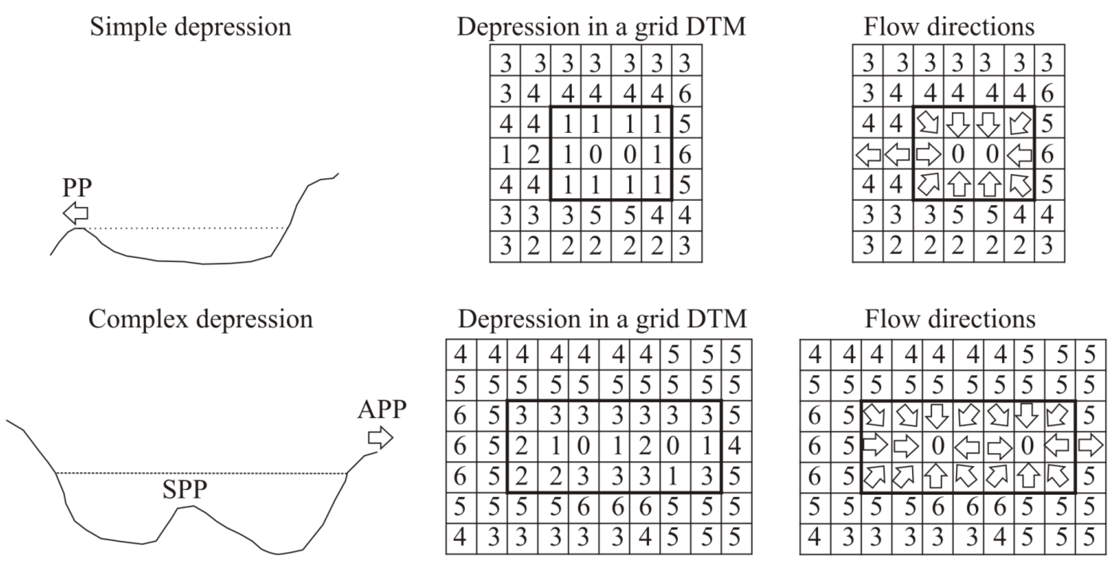
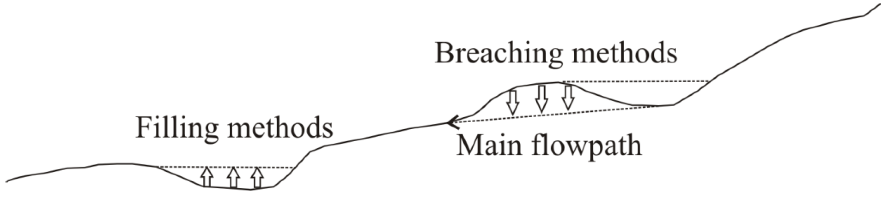
2. Background


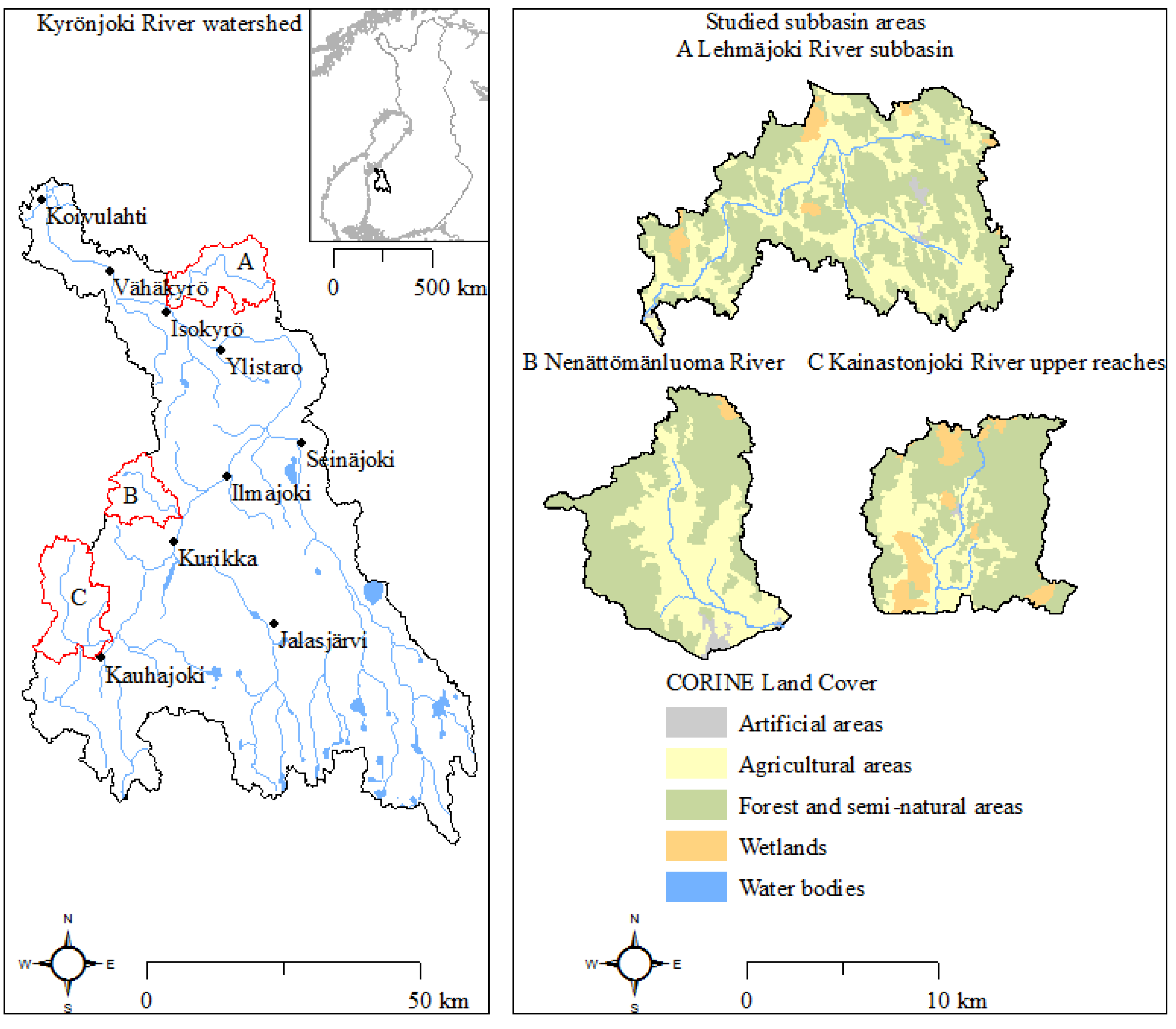
3. Study Areas

4. Materials and Methods
4.1. Field Survey Data
4.2. Laser Scanning Data
4.3. Conventional Nationwide DTMs

4.4. Input Data Processing

| Line | Code |
|---|---|
| 1 | For b ← [cells on data boundary] |
| 2 | Spill[b] ← Elevation[b] |
| 3 | OPEN.push(Spill[b]) |
| 4 | While OPEN is not empty |
| 5 | c ← OPEN.top() |
| 6 | OPEN.pop(c) |
| 7 | CLOSED[c] ← true |
| 8 | For n ← [neighbours of c] |
| 9 | If n ϵ OPEN or CLOSED[n] = true |
| 10 | Then [do nothing] |
| 11 | Else |
| 12 | Spill[n] ← Max(Elevation[n], Spill[c]) |
| 13 | OPEN.push(n) |
4.5. Statistical Methods
4.6. Error Models
4.7. Detention Area Survey
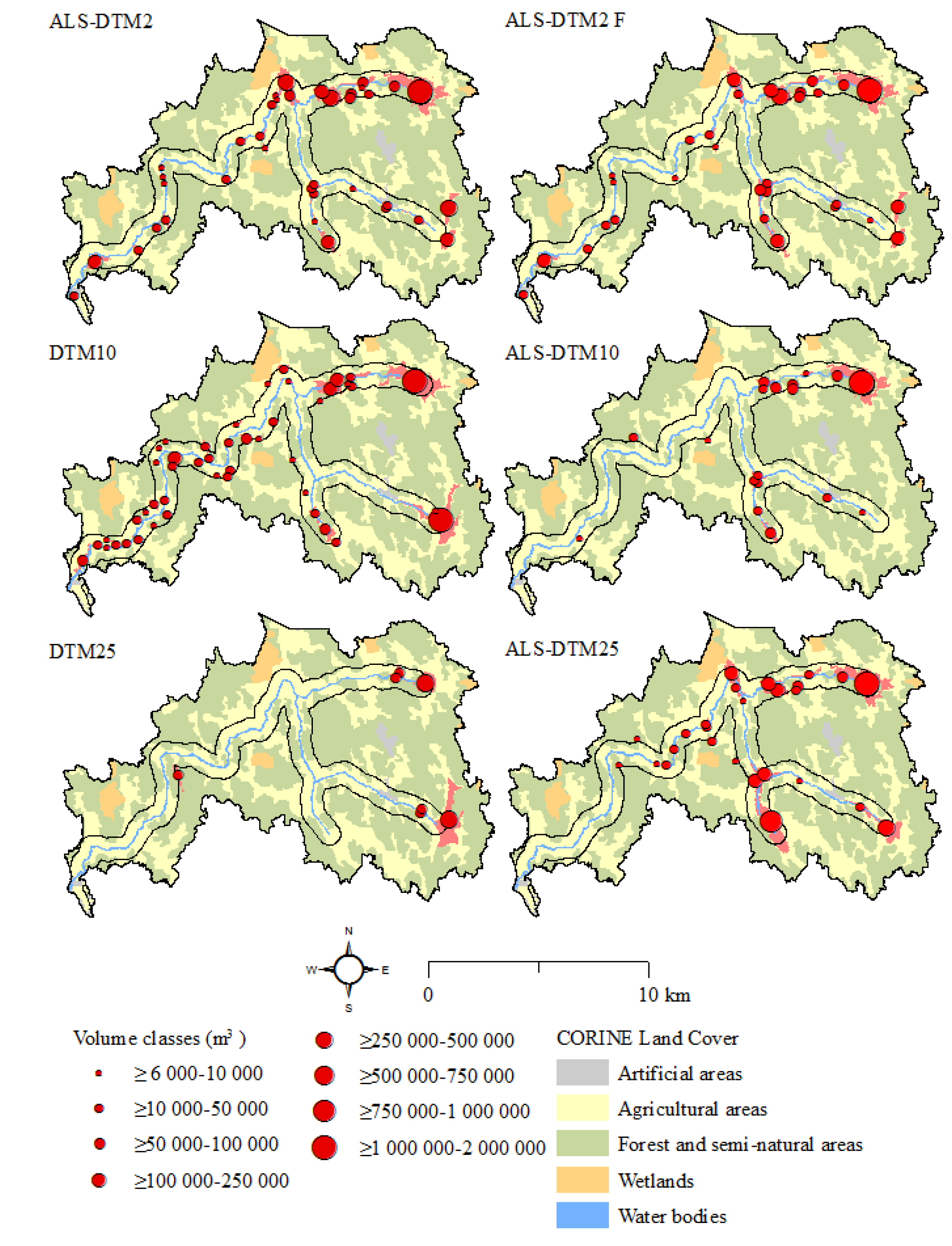
5. Results
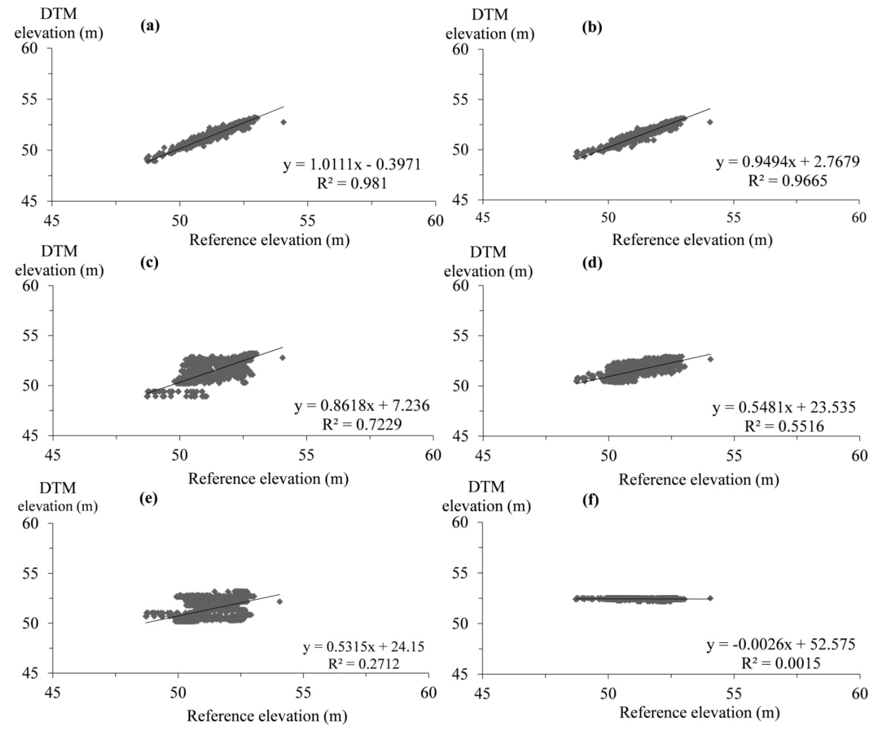
5.1. Accuracy Assessment of Depressions in DTMs Used

| DTM | Area | N | Minimum dz (m) | Maximum dz (m) | Absolute mean error (m) | RMSE (m) | NSE |
|---|---|---|---|---|---|---|---|
| ALS-DTM2 | A | 2355 | −2.27 | 4.097 | 0.230 | 0.406 | 0.958 |
| ALS-DTM2 F | A | 2355 | −2.29 | 4.279 | 0.249 | 0.426 | 0.951 |
| DTM10 | A | 2355 | −4.32 | 3.599 | 0.949 | 1.183 | 0.480 |
| ALS-DTM10 | A | 2355 | −3.90 | 4.029 | 0.521 | 0.839 | 0.816 |
| DTM25 | A | 2355 | −6.62 | 3.345 | 2.641 | 3.318 | −0.594 |
| ALS-DTM25 | A | 2355 | −5.69 | 5.259 | 0.998 | 1.601 | 0.375 |
| ALS-DTM2 | B | 2836 | −1.03 | 1.132 | 0.184 | 0.214 | 0.949 |
| ALS-DTM2 F | B | 2836 | −1.01 | 1.313 | 0.200 | 0.243 | 0.927 |
| DTM10 | B | 2836 | 0.00 | 1.408 | 0.540 | 0.728 | 0.130 |
| ALS-DTM10 | B | 2836 | −2.42 | 2.309 | 0.337 | 0.528 | 0.684 |
| DTM25 | B | 2836 | −3.76 | 1.557 | 1.261 | 1.538 | −0.556 |
| ALS-DTM25 | B | 2836 | −2.74 | 2.207 | 0.595 | 0.918 | 0.058 |
| ALS-DTM2 | C | 731 | −2.22 | 1.298 | 0.238 | 0.321 | 0.966 |
| ALS-DTM2 F | C | 731 | −2.08 | 1.428 | 0.265 | 0.352 | 0.954 |
| DTM10 | C | 731 | −4.73 | 2.103 | 1.040 | 1.492 | −0.574 |
| ALS-DTM10 | C | 731 | −3.37 | 3.349 | 0.609 | 0.899 | 0.710 |
| DTM25 | C | 731 | −5.41 | 1.472 | 1.802 | 2.493 | −0.999 |
| ALS-DTM25 | C | 731 | −5.27 | 4.175 | 1.093 | 1.594 | 0.202 |
| ALS-DTM2 | D | 578 | −2.77 | 1.045 | 0.259 | 0.391 | 0.933 |
| ALS-DTM2 F | D | 578 | −2.51 | 1.317 | 0.326 | 0.464 | 0.896 |
| DTM10 | D | 578 | −3.13 | 1.549 | 1.484 | 1.698 | −0.368 |
| ALS-DTM10 | D | 578 | −3.83 | 2.697 | 0.731 | 1.161 | 0.459 |
| DTM25 | D | 578 | −3.65 | 1.895 | 2.038 | 2.369 | −0.679 |
| ALS-DTM25 | D | 578 | −3.73 | 3.656 | 1.196 | 1.643 | −0.202 |
| ALS-DTM2 | E | 922 | −1.81 | 0.825 | 0.174 | 0.324 | 0.954 |
| ALS-DTM2 F | E | 922 | −1.73 | 1.071 | 0.214 | 0.357 | 0.939 |
| DTM10 | E | 922 | −2.89 | 4.380 | 1.000 | 1.290 | −0.052 |
| ALS-DTM10 | E | 922 | −3.17 | 2.533 | 0.428 | 0.741 | 0.749 |
| DTM25 | E | 922 | −3.86 | 1.935 | 1.456 | 1.923 | −1.866 |
| ALS-DTM25 | E | 922 | −3.37 | 4.793 | 1.224 | 1.606 | −0.844 |
| ALS-DTM2 | F | 865 | −1.57 | 5.656 | 0.134 | 0.294 | 0.977 |
| ALS-DTM2 F | F | 865 | −1.56 | 5.618 | 0.160 | 0.323 | 0.971 |
| DTM10 | F | 865 | −1.92 | 5.734 | 1.121 | 1.368 | −0.825 |
| ALS-DTM10 | F | 865 | −3.09 | 5.678 | 0.349 | 0.585 | 0.906 |
| DTM25 | F | 865 | −5.54 | 4.867 | 2.434 | 3.091 | −0.734 |
| ALS-DTM25 | F | 865 | −4.87 | 5.362 | 0.810 | 1.311 | 0.510 |
| ALS-DTM2 | G | 1734 | −0.98 | 2.234 | 0.104 | 0.176 | 0.982 |
| ALS-DTM2 F | G | 1734 | −1.06 | 2.151 | 0.123 | 0.202 | 0.976 |
| DTM10 | G | 1734 | −3.58 | 3.776 | 1.018 | 1.271 | 0.203 |
| ALS-DTM10 | G | 1734 | −2.79 | 2.735 | 0.307 | 0.543 | 0.851 |
| DTM25 | G | 1734 | −5.03 | 1.519 | 3.904 | 4.115 | −0.161 |
| ALS-DTM25 | G | 1734 | −4.35 | 4.078 | 0.768 | 1.250 | 0.305 |
| DTM/Area | A | B | C | D | E | F | G |
|---|---|---|---|---|---|---|---|
| ALS-DTM2 | 0.9633 | 0.9810 | 0.9782 | 0.9468 | 0.9594 | 0.9776 | 0.9824 |
| ALS-DTM2 F | 0.9590 | 0.9665 | 0.9723 | 0.9327 | 0.9503 | 0.9733 | 0.9773 |
| DTM10 | 0.6697 | 0.5516 | 0.4137 | 0.5587 | 0.3337 | 0.5929 | 0.3709 |
| ALS-DTM10 | 0.8326 | 0.7229 | 0.7429 | 0.5506 | 0.7755 | 0.9111 | 0.8532 |
| DTM25 | 0.0091 | 0.0015 | 0.0030 | 0.0273 | 0.0073 | 0.0005 | 0.0053 |
| ALS-DTM25 | 0.4717 | 0.2712 | 0.3520 | 0.1636 | 0.0995 | 0.6060 | 0.3835 |
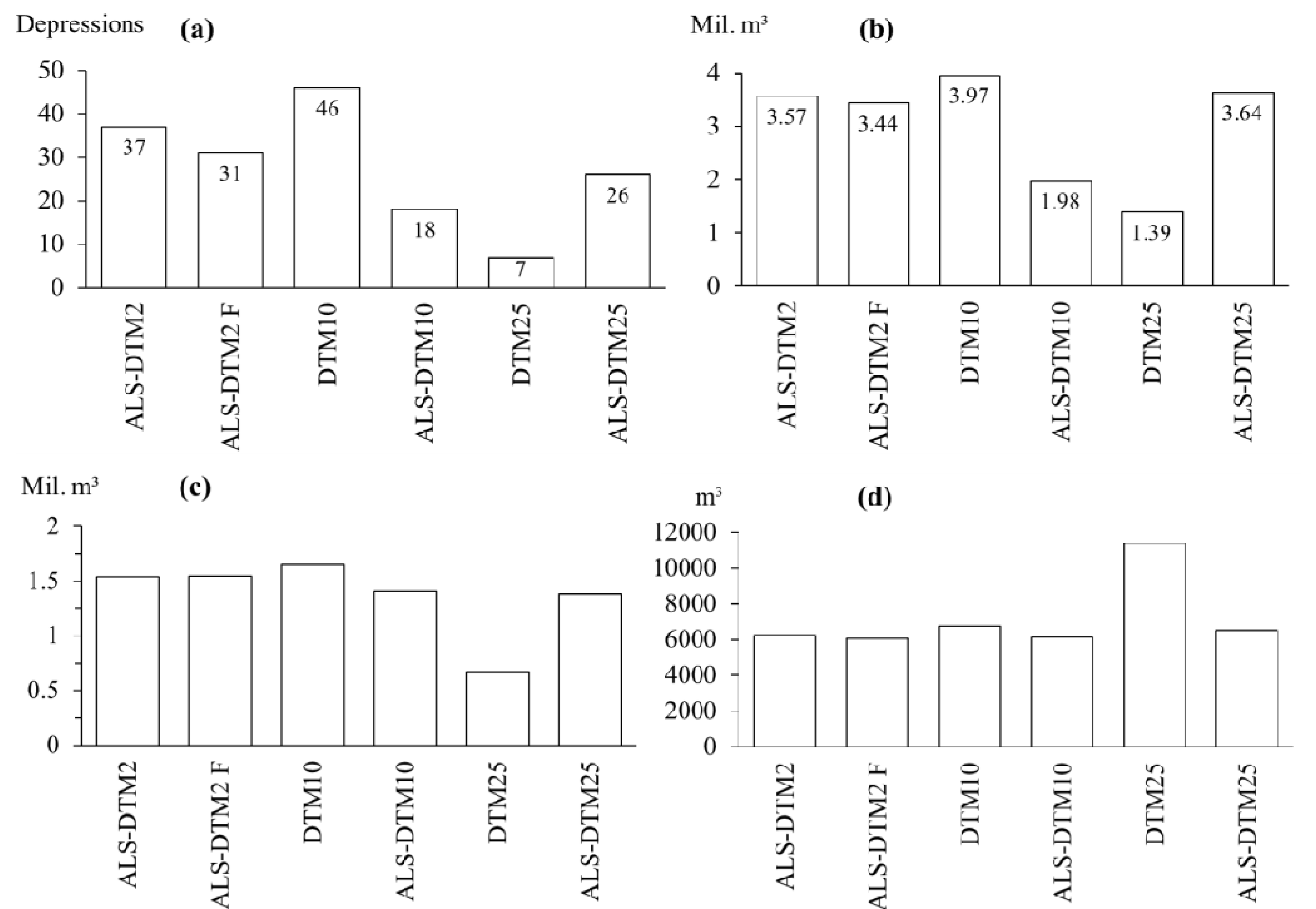
5.2. Depression Variables in DTMs Studied
| DTM/depression type | Depression n | Depression pixel n | Total depression volume (m3) | Total depression area (m2) |
|---|---|---|---|---|
| ALS-DTM2 | ||||
| all depressions | 575,360 | 3,609,277 | 2,603,767 | 14,437,108 |
| shallow depressions | 574,880 | 3,029,933 | 854,636 | 12,119,732 |
| single-pixel depressions | 266,391 | 266,391 | 24,114 | 1,065,564 |
| ALS-DTM2 F | ||||
| all depressions | 199,738 | 2,874,104 | 2,262,584 | 11,496,416 |
| shallow depressions | 199,615 | 2,322,308 | 611,057 | 9,289,232 |
| single-pixel depressions | 63,903 | 63,903 | 2127 | 255,612 |
| DTM10 | ||||
| all depressions | 311 | 37,766 | 1,202,827 | 3,776,600 |
| shallow depressions | 292 | 16,646 | 187,623 | 1,664,600 |
| single-pixel depressions | 41 | 41 | 61 | 4,100 |
| ALS-DTM10 | ||||
| all depressions | 46,257 | 112,383 | 2,752,926 | 11,238,300 |
| shallow depressions | 39,544 | 84,463 | 988,415 | 8,446,300 |
| single-pixel depressions | 32,264 | 32,264 | 473,651 | 2,528,125 |
| DTM25 | ||||
| all depressions | 946 | 3,127 | 214,935 | 1,954,375 |
| shallow depressions | 944 | 3,048 | 191,498 | 1,905,000 |
| single-pixel depressions | 597 | 597 | 37,312 | 373,125 |
| ALS-DTM25 | ||||
| all depressions | 5,268 | 12,250 | 2,263,789 | 7,656,250 |
| shallow depressions | 4,248 | 8,409 | 705,231 | 5,255,625 |
| single-pixel depressions | 4,045 | 4,045 | 473,651 | 2,528,125 |
| DTM | Depression area/km2 | Depressions/km2 | % depression area of SBA | Depressions/one pixel of SBA |
|---|---|---|---|---|
| ALS-DTM2 | 166,422 | 6,632 | 16.6 | 0.0265 |
| ALS-DTM2 F | 132,249 | 2,298 | 13.2 | 0.0092 |
| DTM10 | 43,534 | 4 | 4.4 | 0.0004 |
| ALS-DTM10 | 129,548 | 533 | 13.0 | 0.0533 |
| DTM25 | 22,531 | 11 | 2.3 | 0.0068 |
| ALS-DTM25 | 88,256 | 61 | 8.8 | 0.0380 |
| (a) | ALS-DTM2 | ALS-DTM2 F | ||||||
|---|---|---|---|---|---|---|---|---|
| Pixels/depression | Mean depth (m) | Volume (m3) | Area (m2) | Pixels/depression | Mean depth (m) | Volume (m3) | Area (m2) | |
| Mean | 9.34 | 0.03 | 10.75 | 37.37 | 23.31 | 0.02 | 29.69 | 93.23 |
| Median | 2.00 | 0.02 | 0.13 | 8.00 | 3.00 | 0.01 | 0.13 | 12.00 |
| Mode | 1.000 | 0.002 | 0.008 | 4.000 | 1.000 | 0.001 | 0.004 | 4.000 |
| SDE | 772.02 | 0.04 | 2,330.56 | 3,088.07 | 1,363.55 | 0.03 | 4,071.90 | 5,454.19 |
| Minimum | 1.000 | 0.001 | 0.004 | 4.000 | 1.000 | 0.001 | 0.004 | 4.000 |
| Maximum | 493,837 | 3.72 | 1,662,117 | 1,975,348 | 497,226 | 3.72 | 1,667,566 | 1,988,904 |
| Percentiles | ||||||||
| 25 | 1.000 | 0.008 | 0.040 | 4.000 | 1.000 | 0.005 | 0.031 | 4.000 |
| 75 | 4.00 | 0.04 | 0.46 | 16.00 | 8.00 | 0.02 | 0.64 | 32.00© |
| (b) | DTM10 | ALS-DTM10 | ||||||
| Pixels/depression | Mean depth (m) | Volume (m3) | Area (m2) | Pixels/depression | Mean depth (m) | Volume (m3) | Area (m2) | |
| Mean | 57.49 | 0.11 | 2,604.54 | 5,748.826 | 3.63 | 0.14 | 119.19 | 363.02 |
| Median | 9.00 | 0.06 | 45.35 | 900.00 | 1.00 | 0.06 | 9.20 | 100.00 |
| Mode | 1.000 | 0.002 | 0.200 | 100.000 | 1.000 | 0.007 | 0.700 | 100.000 |
| SDE | 427.14 | 0.18 | 34,961.60 | 42,713.77 | 85.81 | 0.20 | 6,912.35 | 8,581.18 |
| Minimum | 1.000 | 0.001 | 0.100 | 100.000 | 1.000 | 0.001 | 0.100 | 100.000 |
| Maximum | 17,954 | 3.34 | 1,684,317 | 1,795,400 | 18,676 | 3.54 | 1,524,178 | 1,867,600 |
| Percentiles | ||||||||
| 25 | 2.000 | 0.002 | 5.599 | 200.000 | 1.000 | 0.023 | 2.800 | 100.000 |
| 75 | 30.00 | 0.14 | 359.38 | 3,000 | 2.00 | 0.18 | 30.80 | 200.000 |
| (c) | DTM25 | ALS-DTM25 | ||||||
| Pixels/depression | Mean depth (m) | Volume (m3) | Area (m2) | Pixels/depression | Mean depth (m) | Volume (m3) | Area (m2) | |
| Mean | 3.81 | 0.10 | 532.96 | 2,381.27 | 4.10 | 0.19 | 1,082.06 | 2,561.96 |
| Median | 1.00 | 0.10 | 62.50 | 625.00 | 1.00 | 0.10 | 80.63 | 625.00 |
| Mode | 1.000 | 0.100 | 62.499 | 625.000 | 1.000 | 0.004 | 2.500 a | 625.000 |
| SDE | 41.64 | 0.03 | 13,499.30 | 26,024.013 | 52.94 | 0.26 | 23,446.43 | 33,090.2014 |
| Minimum | 1.000 | 0.100 | 62.500 | 625.000 | 1.000 | 0.001 | 0.625 | 625.000 |
| Maximum | 2,729 | 1.43 | 671,376 | 1,705,625 | 2,992 | 2.52 | 1,480,272 | 1,870,000 |
| Percentiles | ||||||||
| 25 | 1.00 | 0.10 | 62.50 | 625.00 | 1.00 | 0.04 | 25.63 | 625.00 |
| 75 | 2.25 | 0.10 | 187.50 | 1,406.25 | 2.00 | 0.24 | 248.13 | 1,250.00 |
5.3. Statistical Methods
| (a) | Kauhajoki River upper reaches | Lehmäjoki River watershed | Nenättömänluoma River watershed | |||
|---|---|---|---|---|---|---|
| Pixel/depression | p < 0.001 | p < 0.001 | p < 0.001 | |||
| Volume of a depression | p < 0.001 | p < 0.001 | p < 0.001 | |||
| Area of a depression | p < 0.001 | p < 0.001 | p < 0.001 | |||
| Mean depth of a depression | p < 0.001 | p < 0.001 | p < 0.001 | |||
| (b) | ALS-DTM2 | ALS-DTM2 F | DTM10 | ALS-DTM10 | DTM25 | ALS-DTM25 |
| Pixel/depression | p < 0.001 | p < 0.001 | p < 0.001 | p < 0.001 | p < 0.001 | p < 0.001 |
| Volume of a depression | p < 0.001 | p < 0.001 | p < 0.001 | p = 0.104 | p < 0.001 | p < 0.001 |
| Area of a depression | p < 0.001 | p < 0.001 | p < 0.001 | p < 0.001 | p < 0.001 | p < 0.001 |
| Mean depth of a depression | p < 0.001 | p < 0.001 | p < 0.001 | p < 0.001 | p < 0.001 | p < 0.001 |
| (a) | Trend | |||||
|---|---|---|---|---|---|---|
| ALS-DTM2 | ALS-DTM2 F | DTM10 | DTM25 | ALS-DTM10 | ALS-DTM25 | |
| Lehmäjoki River and Kainastonjoki River SBAs | ||||||
| Pixels/depression | -/* | -/*** | -/*** | -/X | -/*** | -/*** |
| Volume | */*** | */*** | X/*** | X/*** | */*** | */X |
| Area | ***/* | **/*** | */X | X/*** | ***/*** | **/*** |
| Mean depth | ***/*** | X/*** | ***/*** | X/*** | ***/*** | X/*** |
| Kainastonjoki River and Nenättömänluoma River SBAs | ||||||
| Pixels/depression | -/*** | -/*** | -/X | -/X | -/*** | -/*** |
| Volume | X/*** | X/*** | X/X | X/* | X/*** | X/X |
| Area | X/*** | X/*** | X/X | **/X | X/*** | X/*** |
| Mean depth | ***/*** | X/*** | **/* | X/** | ***/*** | ***/** |
| Lehmäjoki River and Nenättömänluoma River SBAs | ||||||
| Pixels/depression | -/*** | -/*** | -/*** | -/*** | -/*** | -/*** |
| Volume | X/*** | X/*** | X/X | X/*** | X/*** | */* |
| Area | ***/*** | ***/*** | **/*** | */*** | ***/*** | ***/*** |
| Mean depth | ***/*** | X/*** | X/*** | */*** | ***/*** | ***/*** |
| (b) | Trend | |||||
| ALS-DTM2 | ALS-DTM2 F | DTM10 | DTM25 | ALS-DTM10 | ALS-DTM25 | |
| Depression volume (upper part) and area (lower part) in Kainastonjoki River | ||||||
| ALS-DTM2 | X/*** | **/*** | ***/*** | ***/*** | ***/*** | |
| ALS-DTM2 F | ***/*** | **/*** | ***/*** | ***/*** | ***/*** | |
| DTM10 | ***/*** | ***/*** | **/*** | **/*** | */*** | |
| DTM25 | ***/*** | ***/*** | ***/*** | ***/*** | ***/*** | |
| ALS-DTM10 | ***/*** | ***/*** | ***/* | ***/*** | X/X | |
| ALS-DTM25 | ***/*** | ***/*** | ***/*** | ***/*** | **/*** | |
| Depression mean depth (upper part) and pixels per depression (lower part) in Kainastonjoki River SBA | ||||||
| ALS-DTM2 | ***/*** | ***/*** | ***/*** | ***/*** | ***/*** | |
| ALS-DTM2 F | -/*** | ***/*** | ***/*** | ***/*** | ***/*** | |
| DTM10 | -/*** | -/*** | ***/*** | ***/*** | ***/X | |
| DTM25 | -/*** | -/*** | -/*** | ***/*** | ***/*** | |
| ALS-DTM10 | -/*** | -/*** | -/*** | -/*** | ***/*** | |
| ALS-DTM25 | -/*** | -/*** | -/*** | -/*** | -/*** | |
| Depression volume (upper part) and area (lower part) in Lehmäjoki River SBA | ||||||
| ALS-DTM2 | */*** | ***/*** | ***/*** | **/*** | ***/*** | |
| ALS-DTM2 F | ***/*** | ***/*** | **/*** | **/*** | ***/*** | |
| DTM10 | ***/*** | ***/*** | ***/*** | ***/*** | */*** | |
| DTM25 | ***/*** | ***/*** | ***/*** | */*** | ***/*** | |
| ALS-DTM10 | ***/*** | ***/*** | ***/*** | ***/*** | X/*** | |
| ALS-DTM25 | ***/*** | ***/*** | ***/X | ***/*** | X/*** | |
| Depression mean depth (upper part) and pixels per depression (lower part) in Lehmäjoki River SBA | ||||||
| ALS-DTM2 | ***/*** | ***/*** | ***/*** | ***/*** | ***/*** | |
| ALS-DTM2 F | -/*** | ***/*** | ***/*** | ***/*** | ***/*** | |
| DTM10 | -/*** | -/*** | ***/*** | **/*** | ***/*** | |
| DTM25 | -/*** | -/*** | -/*** | ***/*** | ***/*** | |
| ALS-DTM10 | -/*** | -/*** | -/*** | -/*** | ***/* | |
| ALS-DTM25 | -/*** | -/*** | -/*** | -/*** | -/*** | |
| Depression volume (upper part) and area (lower part) in Nenättömänluoma River SBA | ||||||
| ALS-DTM2 | */*** | **/*** | ***/*** | ***/*** | ***/*** | |
| ALS-DTM2 F | ***/*** | **/*** | ***/*** | ***/*** | ***/*** | |
| DTM10 | ***/*** | ***/*** | **/*** | **/*** | **/X | |
| DTM25 | ***/*** | ***/*** | ***/*** | X/*** | ***/*** | |
| ALS-DTM10 | ***/*** | ***/*** | ***/*** | ***/*** | **/X | |
| ALS-DTM25 | ***/*** | ***/*** | ***/*** | ***/*** | X/*** | |
| Depression mean depth (upper part) and pixels per depression (lower part) in Nenättömänluoma River SBA | ||||||
| ALS-DTM2 | ***/*** | ***/*** | ***/*** | ***/*** | ***/*** | |
| ALS-DTM2 F | -/*** | ***/*** | ***/*** | ***/*** | ***/*** | |
| DTM10 | -/*** | -/*** | ***/*** | X/*** | ***/*** | |
| DTM25 | -/*** | -/*** | -/*** | ***/*** | ***/*** | |
| ALS-DTM10 | -/*** | -/*** | -/*** | -/*** | ***/*** | |
| ALS-DTM25 | -/*** | -/*** | -/*** | -/X | -/*** | |
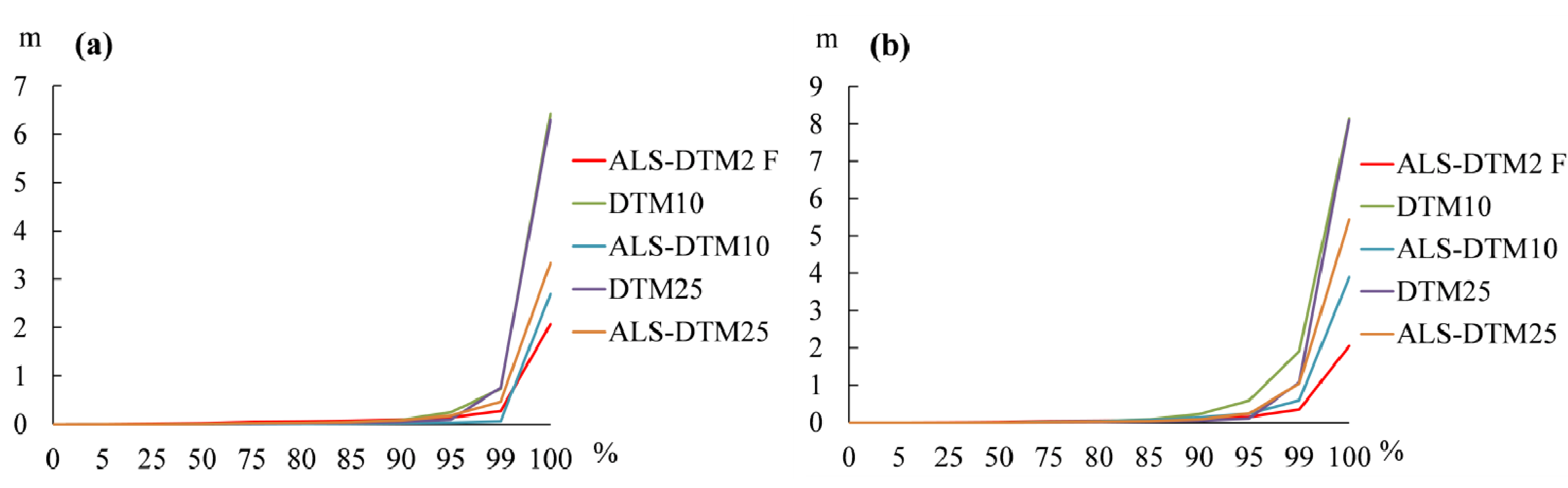
5.4. Error Models
| Area/DTM | Maximum (m) | Mean (m) | SD (m) | Median (m) | Surface areas of error in SBAs (%) |
|---|---|---|---|---|---|
| Kainastonjoki | |||||
| ALS-DTM2 F | 2.07 | 0.007 | 0.03 | 0.023 | 19.1 |
| DTM10 | 6.43 | 0.03 | 0.18 | 0.007 | 63.1 |
| ALS-DTM10 | 2.69 | 0.03 | 0.09 | 0.002 | 35.9 |
| DTM25 | 6.32 | 0.03 | 0.18 | 0.006 | 84.3 |
| ALS-DTM25 | 3.33 | 0.03 | 0.10 | 0.007 | 84.4 |
| Nenättömänluoma | |||||
| ALS-DTM2 F | 2.05 | 0.005 | 0.04 | 0.019 | 13.5 |
| DTM10 | 8.14 | 0.06 | 0.33 | 0.006 | 48.2 |
| ALS-DTM10 | 3.89 | 0.02 | 0.11 | 0.006 | 47.1 |
| DTM25 | 8.10 | 0.04 | 0.28 | 0.004 | 66.7 |
| ALS-DTM25 | 5.44 | 0.04 | 0.19 | 0.005 | 66.8 |
| Lehmäjoki | |||||
| ALS-DTM2 F | 1.54 | 0.01 | 0.04 | 0.025 | 21.1 |
| DTM10 | 5.03 | 0.07 | 0.22 | 0.011 | 59.1 |
| ALS-DTM10 | 3.52 | 0.04 | 0.12 | 0.008 | 56.2 |
| DTM25 | 5.44 | 0.06 | 0.24 | 0.008 | 77.7 |
| ALS-DTM25 | 3.71 | 0.03 | 0.10 | 0.008 | 76.9 |

5.5. Survey of Detention Areas for Water

6. Discussion
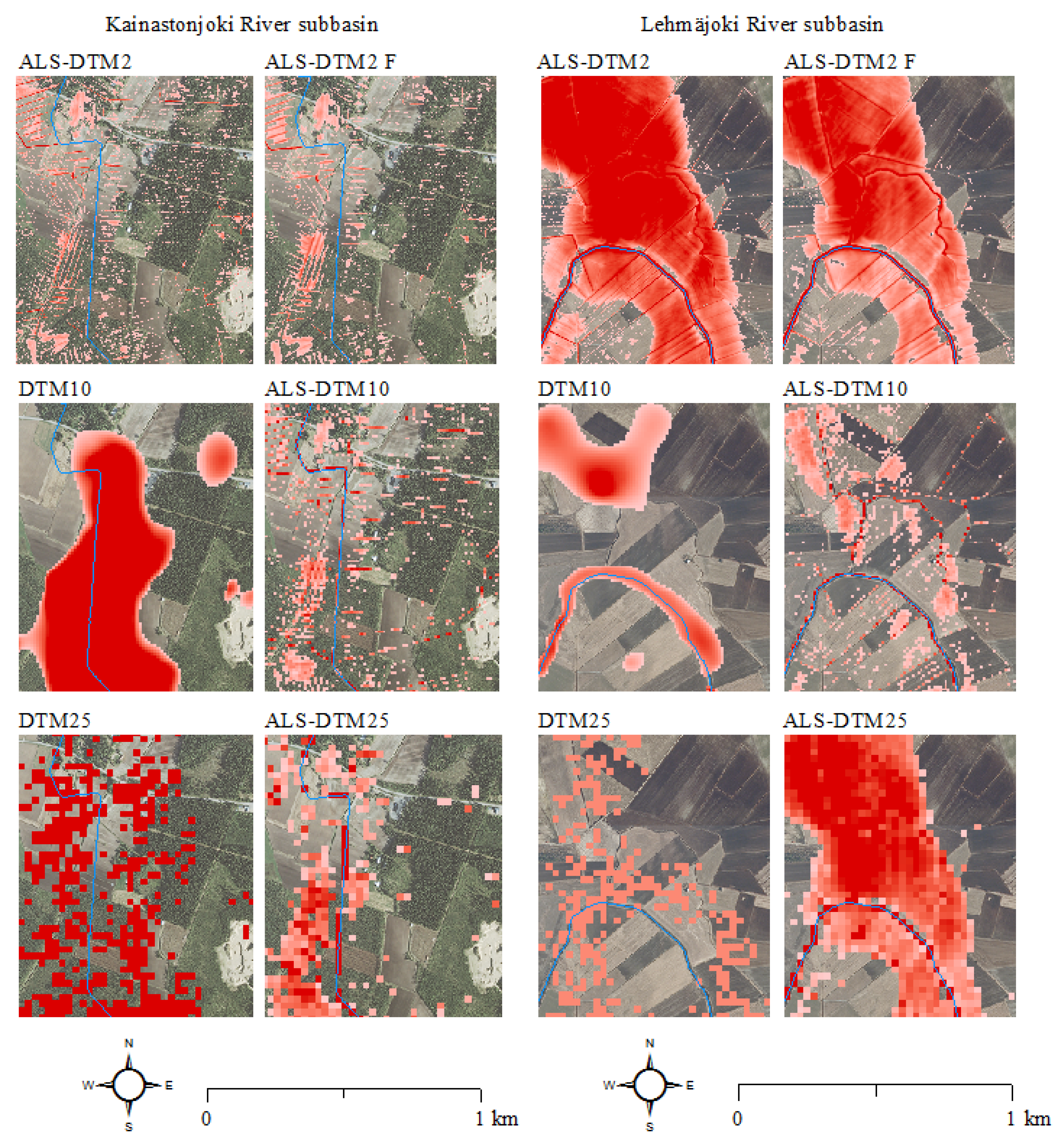
6.1. The Accuracy of DTMs for Representing Terrain
6.2. The Variation of the Hydrological Depression Variables
6.3. Error Models and Detention Area Survey
7. Conclusions
- ▪
- ALS-DTMs are closer to the real topography of depressions than DTMs based on more conventional acquisition and processing methods. The accuracy of terrain representation decreased with increasing grid size in both groups of DTMs.
- ▪
- The acquisition method, processing method and grid size of a DTM has an impact on modelled depression variables. This variation was found to be area, acquisition method, processing method and scale dependent.
- The difference between ALS-DTM10 and DTM10 is the largest. The principal reason was the scattered depression pixels that were great in number because of the resampling process performed. The number of these separate fragmental pixels decreased as the degree of terrain representation became greater with increasing grid size. DTM10 also differed from the other DTMs in terms of statistical significance.
- The absolute number of depressions and depression pixels is larger in ALS-DTM10 and ALS-DTM25 than in DTM10 and DTM25. This is a consequence of the resampling process of ALS-DTM2 that produces scattered depression pixels.
- The mean filtering of ALS-DTM2 focuses on the small and shallow depressions, and is thus suitable for detection of water detention areas in flood risk management.
- ▪
- The maximum pixel depth error of a DTM illustrated the amount of depth error in relation to ALS-DTM2 in a most descriptive way. ALS-DTMs have smaller maximum error values than the nationwide NLS grid DTMs 10 m × 10 m and 25 m × 25 m.
- ▪
- The accuracy of DTMs in representing separate depressions varied. Thus, the decreasing grid size of a DTM is no guarantee of increasing spatial accuracy when there is a demand for the most accurate data available. According to the aforementioned findings, the acquisition method, processing method and grid size of a DTM have an impact on the location, number and total volumes of depression areas.
Appendix
| Area/DTM | Depression number | Median mean depth (m) | SD mean depth (m) | Median volume (m3) | SD volume (m3) | Max depth (m) |
|---|---|---|---|---|---|---|
| Upper reaches of Kainastonjoki River SBA | ||||||
| ALS-DTM2 | 266,391 | 0.01 (0.02) | 0.03 | 0.05 (0.09) | 0.12 | 0.51 |
| ALS-DTM2 F | 63,903 | 0.005 (0.008) | 0.01 | 0.02 (0.03) | 0.04 | 0.19 |
| DTM10 | 41 | 0.003 (0.01) | 0.05 | 0.30 (1.49) | 5.29 | 0.34 |
| DTM25 | 597 | 0.10 (0.10) | 0.000002 | 62.50 (62.50) | 0.001 | 0.10 |
| ALS-DTM10 | 32,264 | 0.08 (0.15) | 0.19 | 7.80 (14.98) | 18.91 | 2.74 |
| ALS-DTM25 | 4045 | 0.10 (0.19) | 0.25 | 64.38 (117.10) | 156.08 | 4.51 |
| Nenättömänluoma River SBA | ||||||
| ALS-DTM2 | 266,830 | 0.01 (0.02) | 0.03 | 0.04 (0.03) | 0.12 | 0.47 |
| ALS-DTM2 F | 55,901 | 0.005 (0.009) | 0.01 | 0.02 (0.01) | 0.04 | 0.19 |
| DTM10 | 50 | 0.004 (0.01) | 0.02 | 0.40 (0.98) | 2.25 | 0.15 |
| DTM25 | 954 | 0.10 (0.10) | 0.01 | 62.50 (62.83) | 6.71 | 0.40 |
| ALS-DTM10 | 29,459 | 0.07 (0.17) | 0.22 | 7.50 (16.52) | 22.12 | 2.43 |
| ALS-DTM25 | 3619 | 0.11 (0.22) | 0.30 | 68.75 (137.19) | 186.96 | 3.72 |
| Lehmäjoki River SBA | ||||||
| ALS-DTM2 | 365,225 | 0.01 (0.02) | 0.03 | 0.04 (0.54) | 0.12 | 0.54 |
| ALS-DTM2 F | 76,014 | 0.004 (0.008) | 0.01 | 0.02 (0.15) | 0.04 | 0.15 |
| DTM10 | 701 | 0.01 (0.02) | 0.04 | 1.00 (2.29) | 3.90 | 0.55 |
| DTM25 | 3178 | 0.10 (0.10) | 0.01 | 62.50 (62.18) | 7.68 | 0.60 |
| ALS-DTM10 | 40,073 | 0.05 (0.14) | 0.21 | 5.20 (13.98) | 21.05 | 2.37 |
| ALS-DTM25 | 5854 | 0.08 (0.19) | 0.26 | 52.50 (116.97) | 160.63 | 2.42 |
| Area/DTM | Depression number | Depression pixel number | Median mean depth (m) | SD mean depth (m) | Median volume (m3) | SD volume (m3) | Median area (m2) | SD area (m2) |
|---|---|---|---|---|---|---|---|---|
| Upper reaches of Kainastonjoki River SBA | ||||||||
| ALS-DTM2 | 574,880 | 3,029,933 | 0.02 (0.03) | 0.04 | 0.14 (1.49) | 40.46 | 8.00 (21.08) | 309.68 |
| ALS-DTM2F | 199,615 | 2,322,308 | 0.01 (0.02) | 0.02 | 0.12 (3.06) | 81.94 | 12.00 (46.54) | 397.37 |
| DTM10 | 292 | 16,646 | 0.03 (0.05) | 0.06 | 29.50 (642.55) | 2,357.16 | 1350 (5,700.68) | 13,931.44 |
| DTM25 | 944 | 3048 | 0.10 (0.10) | 0.006 | 62.50 (202.86) | 496.20 | 625 (2018) | 4,869.32 |
| ALS-DTM10 | 39,544 | 84,463 | 0.07 (0.09) | 0.08 | 9.20 (25) | 235.30 | 100 (213.59) | 994.02 |
| ALS-DTM25 | 4248 | 8409 | 0.08 (0.10) | 0.08 | 63.12 (166.01) | 1,179.68 | 625 (1,237.20) | 5,150.54 |
| Nenättömänluoma River SBA | ||||||||
| ALS-DTM2 | 514,387 | 2,260,555 | 0.02 (0.03) | 0.03 | 0.11 (1.08) | 34.20 | 4.00 (17.58) | 162.14 |
| ALS-DTM2F | 156,593 | 1,573,508 | 0.01 (0.02) | 0.02 | 0.10 (2.34) | 45.92 | 12.00 (40.19) | 260.31 |
| DTM10 | 434 | 31,456 | 0.03 (0.06) | 0.07 | 40.80 (1,124.32) | 4,052.12 | 1500 (7,247.93) | 18,371.54 |
| DTM25 | 1462 | 3077 | 0.10 (0.10) | 0.004 | 62.50 (1,315.41) | 234.39 | 625 (1,315.4) | 2,253.94 |
| ALS-DTM10 | 31,026 | 55,190 | 0.06 (0.08) | 0.08 | 7.00 (18.33) | 147.74 | 100 (177.88) | 715.02 |
| ALS-DTM25 | 3445 | 5278 | 0.08 (0.10) | 0.08 | 55.63 (111.19) | 383.61 | 625 (957.55) | 1,784.74 |
| Lehmäjoki River SBA | ||||||||
| ALS-DTM2 | 777,433 | 4,916,916 | 0.02 (0.03) | 0.03 | 0.13 (1.89) | 88.50 | 8.00 (25.30) | 487.48 |
| ALS-DTM2F | 249,806 | 3,683,152 | 0.01 (0.02) | 0.02 | 0.13 (4.12) | 112.42 | 12.00 (58.98) | 605.74 |
| DTM10 | 3630 | 108,636 | 0.05 (0.07) | 0.07 | 33.20 (479.81) | 2,922.84 | 750 (2,992.73) | 112.90 |
| DTM25 | 5293 | 15,686 | 0.10 (0.10) | 0.008 | 62.50 (195.81) | 838.97 | 625 (1,852.20) | 4,851.34 |
| ALS-DTM10 | 50,649 | 139,039 | 0.05 (0.08) | 0.07 | 6.60 (29.97) | 475.64 | 100 (274.51) | 1,885.08 |
| ALS-DTM25 | 6531 | 15,470 | 0.07 (0.09) | 0.08 | 53.13 (185.38) | 1,012.33 | 625 (1,480.44) | 4,040.79 |
Acknowledgments
Conflicts of Interest
References
- Wang, L.; Liu, H. An efficient method for identifying and filling surface depressions in digital elevation models for hydrologic analysis and modelling. Int. J. Geogr. Inf. Sci. 2006, 20, 193–213. [Google Scholar]
- Liu, H.; Wang, L. Mapping detention basins and deriving their spatial attributes from airborne LiDAR data for hydrological applications. Hydrol. Process. 2008, 22, 2358–2369. [Google Scholar] [CrossRef]
- Alho, P.; Hyyppä, H.; Hyyppä, J. Consequence of DTM precision for flood hazard mapping: A case study in SW Finland. Nord.J.Surv.Real Estate Res. 2009, 6, 21–39. [Google Scholar]
- Dhun, K. Application of LiDAR DEMs to the Modelling of Surface Drainage Patterns in Human Modified Landscapes; The University of Guelph: Guelph, ON, Canada, 2011. [Google Scholar]
- Wang, L.; Yu, J. Modelling detention basins measured from high-resolution light detection and ranging data. Hydrol. Process. 2012, 26, 2973–2984. [Google Scholar] [CrossRef]
- Hilldale, R.C.; Raff, D. Assessing the ability of airborne LiDAR to map river bathymetry. Earth Surf. Processes 2008, 33, 773–783. [Google Scholar] [CrossRef]
- Alho, P.; Kukko, A.; Hyyppä, H.; Kaartinen, H.; Hyyppä, J.; Jaakkola, A. Application of boat-based laser scanning for river survey. Earth Surf. Processes 2009, 34, 1831–1838. [Google Scholar] [CrossRef]
- Vaaja, M.; Hyyppä, J.; Kukko, A.; Kaartinen, H.; Hyyppä, H.; Alho, P. Mapping topography changes and elevation accuracies using a mobile laser scanner. Remote Sens. 2011, 3, 587–600. [Google Scholar] [CrossRef]
- Bolstad, P.V.; Stowe, T. An evaluation of DEM accuracy—Elevation, slope, and aspect. Photogramm. Eng. RemoteSens. 1994, 60, 1327–1332. [Google Scholar]
- Thompson, J.A.; Bell, J.C.; Butler, C.A. Digital elevation model resolution: Effects on terrain attribute calculation and quantitative soil-landscape modeling. Geoderma 2001, 100, 67–89. [Google Scholar] [CrossRef]
- Burdziej, J.; Kunz, M. Effect of digital terrain model resolution on topographic parameters calculation and spatial distribution of errors. In Proceedings of the 26th Annual Symposium of the European Association of Remote Sensing Laboratories (EARSel), Warsaw, Poland, 29 May–2 June 2006; pp. 615–626.
- Vaze, J.; Teng, J.; Spencer, G. Impact of DEM accuracy and resolution on topographic indices. Environ. Modell. Softw. 2010, 25, 1086–1098. [Google Scholar] [CrossRef]
- Chu, X.; Zhang, J.; Yang, J.; Chi, Y. Quantitative evaluation of the relationship between grid spacing of DEMs and surface depression storage. In Proceedings of the World Environmental and Water Resources Congress 2010: Challenges of Change, Providence, RI, USA, 16–20 May 2010; pp. 4447–4457.
- Haile, A.T.; Rientjes, T. Effects of LiDAR DEM resolution in flood modelling: A model sensitivity study for the city of Tegucigalpa, Honduras. In Proceedings of the ISPRS WG III/3, III/4, V/3 Workshop “Laser scanning 2005”, Enschede, The Netherlands, 12–14 September 2005.
- Wolock, D.M.; Price, C.V. Effects of digital elevation model map scale and data resolution on a topography-based watershed model. Water Resour. Res. 1994, 30, 3041–3052. [Google Scholar] [CrossRef]
- Zhang, W.H.; Montgomery, D.R. Digital elevation model grid size, landscape representation, and hydrologic simulation. Water Resour. Res. 1994, 30, 1019–1028. [Google Scholar] [CrossRef]
- Gyasi-Agyei, Y.; Willgoose, G.; Detroch, F.P. Effects of vertical resolution and map scale of digital elevation models on geomorphological parameters used in hydrology. Hydrol. Process. 1995, 9, 363–382. [Google Scholar] [CrossRef]
- Li, J.; Wong, D.W.S. Effects of DEM sources on hydrologic applications. Comput. Environ. Urban 2010, 34, 251–261. [Google Scholar] [CrossRef]
- Wu, S.; Li, J.; Huang, G.H. Characterization and evaluation of elevation data uncertainty in water resources modeling with gis. Water Resour. Manag. 2008, 22, 959–972. [Google Scholar] [CrossRef]
- Oksanen, J. Digital Elevation Model Error in Terrain Analysis; Academic Dissertation in Geography, University of Helsinki: Helsinki, Finland, 2006. [Google Scholar]
- Oksanen, J. Tracing the gross errors of DEM—Visualisation techniques for preliminary quality analysis. In Proceedings of the 21st International Cartographic Conference, Durban, South Africa, 10–16 August 2003.
- Oksanen, J.; Sarjakoski, T. Uncovering the statistical and spatial characteristics of fine toposcale DEM error. Int. J. Geogr. Inf. Sci. 2006, 20, 345–369. [Google Scholar] [CrossRef]
- Oksanen, J.; Sarjakoski, T. Error propagation analysis of DEM-based drainage basin delineation. Int. J. Remote Sens. 2005, 26, 3085–3102. [Google Scholar] [CrossRef]
- Oksanen, J.; Sarjakoski, T. Error propagation of DEM-based surface derivatives. Comput. Geosci. 2005, 31, 1015–1027. [Google Scholar]
- Abedini, M.J.; Dickinson, W.T.; Rudra, R.P. On depressional storages: The effect of DEM spatial resolution. J. Hydrol. 2006, 318, 138–150. [Google Scholar] [CrossRef]
- Zandbergen, P.A. The effect of cell resolution on depressions in digital elevation models. Appl. GIS 2006, 2. [Google Scholar] [CrossRef]
- Yang, J.; Chu, X. Effects of DEM resolution on surface depression properties and hydrologic connectivity. J. Hydrol. Eng. 2013, 18, 1157–1169. [Google Scholar] [CrossRef]
- Huang, C.; Bradford, J.M. Depressional storage for markov-gaussian surfaces. Water Resour. Res. 1990, 26, 2235–2242. [Google Scholar] [CrossRef]
- Carvajal, F.; Aguilar, M.A.; Aguera, F.; Aguilar, F.J.; Giraldez, J.V. Maximum depression storage and surface drainage network in uneven agricultural landforms. Biosyst.Eng. 2006, 95, 281–293. [Google Scholar] [CrossRef]
- Alvarez-Mozos, J.; Angel Campo, M.; Gimenez, R.; Casali, J.; Leibar, U. Implications of scale, slope, tillage operation and direction in the estimation of surface depression storage. Soil TillageRes. 2011, 111, 142–153. [Google Scholar] [CrossRef]
- Lindsay, J.B.; Creed, I.F. Sensitivity of digital landscapes to artifact depressions in remotely-sensed DEMs. Photogramm. Eng. RemoteSens. 2005, 71, 1029–1036. [Google Scholar] [CrossRef]
- Zandbergen, P.A. Accuracy considerations in the analysis of depressions in medium-resolution LiDAR DEMs. Gisci. Remote Sens. 2010, 47, 187–207. [Google Scholar]
- Ullah, W.; Dickinson, W.T. Quantitative description of depression storage using a digital surface model. 2. Characteristics of surface depressions. J. Hydrol. 1979, 42, 77–90. [Google Scholar] [CrossRef]
- Chi, Y.; Yang, J.; Chu, X. Characterization of surface roughness and computation of depression storage. In Proceedings of the World Environmental and Water Resources Congress 2010: Challenges of Change, Providence, RI, USA, 16–20 May 2010; pp. 4437–4446.
- Yang, J.; Chu, X.; Chi, Y.; Sande, L. Effects of rough surface slopes on surface depression storage. In Proceedings of the World Environmental and Water Resources Congress 2010: Challenges of Change, Providence, RI, USA, 16–20 May 2010; pp. 4427–4436.
- Denmark’s Digital Elevation Model. Available online: http://www.niras.com/Business-Areas/Mapping/Map-products/Denmarks-elevation-model.aspx (accessed on 1 September 2013).
- Fakta om Laserskanning. Available online: http://www.lantmateriet.se/Kartor-och-geografisk-information/Hojddata/Fakta-om-laserskanning/ (accessed on 22 November 2013).
- Pitkän aikavälin laserkeilaussuunnitelma kattaa kattaa vuodet 2014–2019. Available online: http://www.maanmittauslaitos.fi/kartat/laserkeilausaineistot/laserkeilausindeksit/laserkeilaussuunnitelma-2014-2019 (accessed on 1 September 2013).
- Laser Scanning Data. Available online: http://www.maanmittauslaitos.fi/en/maps-5 (accessed on 1 September 2013).
- Ullah, W.; Dickinson, W.T. Quantitative description of depression storage using a digital surface model. 1. Determination of depression storage. J. Hydrol. 1979, 42, 63–75. [Google Scholar] [CrossRef]
- Jenson, S.K.; Domingue, J.O. Extracting topographic structure from digital elevation data for geographic information-system analysis. Photogramm. Eng. RemoteSens. 1988, 54, 1593–1600. [Google Scholar]
- Martz, L.W.; Garbrecht, J. The treatment of flat areas and depressions in automated drainage analysis of raster digital elevation models. Hydrol. Process. 1998, 12, 843–855. [Google Scholar] [CrossRef]
- Rieger, W. A phenomenon-based approach to upslope contributing area and depressions in DEMs. Hydrol. Process. 1998, 12, 857–872. [Google Scholar] [CrossRef]
- Freeman, T.G. Calculating catchment-area with divergent flow based on a regular grid. Comput. Geosci. 1991, 17, 413–422. [Google Scholar] [CrossRef]
- Planchon, O.; Darboux, F. A fast, simple and versatile algorithm to fill the depressions of digital elevation models. Catena 2002, 46, 159–176. [Google Scholar] [CrossRef]
- Ukkonen, T.; Sarjakoski, T.; Oksanen, J. Distributed computation of drainage basin delineations from uncertain digital elevation models. In Proceedings of the 15th Annual ACM International Symposium on Advances in Geographic Information Systems, Seattle, WA, USA, 7–9 November 2007; pp. 236–243.
- Rieger, W. Automated river line and catchment area extraction from DEM data. Int. Arch.Photogramm.Remote Sens. 1993, 29, 642–642. [Google Scholar]
- Lindsay, J.B.; Creed, I.F. Removal of artifact depressions from digital elevation models: Towards a minimum impact approach. Hydrol. Process. 2005, 19, 3113–3126. [Google Scholar] [CrossRef]
- Lindsay, J.B.; Creed, I.F. Distinguishing actual and artefact depressions in digital elevation data. Comput. Geosci. 2006, 32, 1192–1204. [Google Scholar] [CrossRef]
- Mansikkaniemi, H.; Seura, S.M. Sedimentation and water quality in the flood basin of the river Kyrönjoki in Finland. Geogr.Soc.Finl. 1985, 163, 155–194. [Google Scholar]
- Flood Risk Management Planning in Finland. Available online: http://www.environment.fi/en-US/Water_and_sea/Floods/Flood_risk_management/Flood_risk_management_planning (accessed on 20 September 2013).
- Saunders, W. Preparation of DEMs for Use in Environmental Modeling Analysis. In Hydrologic and Hydraulic Modeling Support with Geographic Information Systems; ESRI Press: New York, NY, USA, 2000; pp. 29–52. [Google Scholar]
- Digital Elevation Model 2 m. Available online: http://www.maanmittauslaitos.fi/en/digituotteet/digital-elevation-model-2-m (accessed on 31 January 2013).
- Laserkeilausaineisto. Available online: http://www.maanmittauslaitos.fi/digituotteet/laserkeilausaineisto (accessed on 31 January 2013).
- Vilhomaa, J. Valtakunnallisen korkeusmallin tuotantoprosessin kehitystyö (Development of a production process for a national elevation model). Licentiate’s Thesis, Aalto University, Espoo, Finland, 2008. [Google Scholar]
- Korkeusmalliryhmä. In Valtakunnallisen korkeusmallin uudistamistarpeet ja -vaihtoehdot; Ministry of Agriculture and Forestry: Helsinki, Finland, 2006; p. 76.
- Korkeusmalli 10 m. Available online: http://www.maanmittauslaitos.fi/digituotteet/korkeusmalli-10-m (accessed on 31 January 2013).
- Nash, J.; Sutcliffe, J. River flow forecasting through conceptual models Part I—A discussion of principles. J. Hydrol. 1970, 10, 282–290. [Google Scholar] [CrossRef]
- Moriasi, D.N.; Arnold, J.G.; Van Liew, M.W.; Bingner, R.L.; Harmel, R.D.; Veith, T.L. Model evaluation guidelines for systematic quantification of accuracy in watershed simulations. Trans. ASABE 2007, 50, 885–900. [Google Scholar]
- French, J.R. Critical perspectives on the evaluation and optimization of complex numerical models of estuary hydrodynamics and sediment dynamics. Earth Surf. Processes 2010, 35, 174–189. [Google Scholar]
- Lotsari, E.; Wainwright, D.; Corner, G.D.; Alho, P.; Käyhkö, J. Surveyed and modelled one-year morphodynamics in the braided lower Tana River. Hydrol. Process. 2014, 28, 2685–2716. [Google Scholar] [CrossRef]
- Suomen Salaojakeskus Oy. Ilmajoen tulvariskien hallinnan yleissuunitelma; Suomen Salaojakeskus Oy: Ilmajoki, Finland, 2010; p. 67. [Google Scholar]
- American Society of Civil Engineers. Criteria for evaluation of watershed models. J. Irrig. Drain. Eng. ASCE 1993, 119, 429–442. [Google Scholar]
- Legates, D.R.; McCabe, G.J. Evaluating the use of “goodness-of-fit” measures in hydrologic and hydroclimatic model validation. Water Resour. Res. 1999, 35, 233–241. [Google Scholar] [CrossRef]
- McCuen, R.H.; Knight, Z.; Cutter, A.G. Evaluation of the nash-sutcliffe efficiency index. J. Hydrol. Eng. 2006, 11, 597–602. [Google Scholar] [CrossRef]
- Ahokas, E.; Kaartinen, H.; Hyyppä, J. On the quality checking of the airborne laser scanningbased nationwide elevation model in Finland. Int. Arch. Photogramm. Remote Sens. Spat. Inf. Sci. 2008, 37, 267–270. [Google Scholar]
- Kamphorst, E.C.; Jetten, V.; Guerif, J.; Pitkanen, J.; Iversen, B.V.; Douglas, J.T.; Paz, A. Predicting depressional storage from soil surface roughness. Soil Sci. Soc. Am. J. 2000, 64, 1749–1758. [Google Scholar] [CrossRef]
- Tribe, A. Automated recognition of valley lines and drainage networks from grid digital elevation models—A review and a new method. J. Hydrol. 1992, 139, 263–293. [Google Scholar] [CrossRef]
- Sane, M.; Alho, P.; Huokuna, M.; Käyhkö, J.; Selin, M. Opas yleispiirteisen tulvavaarakartoituksen laatimiseen (Guidelines for flood hazard mapping on a coarse scale); Environment Guide 127; Finnish Environment Institute: Helsinki, Finland, 2006; p. 73. [Google Scholar]
© 2014 by the authors; licensee MDPI, Basel, Switzerland. This article is an open access article distributed under the terms and conditions of the Creative Commons Attribution license (http://creativecommons.org/licenses/by/3.0/).
Share and Cite
Vesakoski, J.-M.; Alho, P.; Hyyppä, J.; Holopainen, M.; Flener, C.; Hyyppä, H. Nationwide Digital Terrain Models for Topographic Depression Modelling in Detection of Flood Detention Areas. Water 2014, 6, 271-300. https://doi.org/10.3390/w6020271
Vesakoski J-M, Alho P, Hyyppä J, Holopainen M, Flener C, Hyyppä H. Nationwide Digital Terrain Models for Topographic Depression Modelling in Detection of Flood Detention Areas. Water. 2014; 6(2):271-300. https://doi.org/10.3390/w6020271
Chicago/Turabian StyleVesakoski, Jenni-Mari, Petteri Alho, Juha Hyyppä, Markus Holopainen, Claude Flener, and Hannu Hyyppä. 2014. "Nationwide Digital Terrain Models for Topographic Depression Modelling in Detection of Flood Detention Areas" Water 6, no. 2: 271-300. https://doi.org/10.3390/w6020271
APA StyleVesakoski, J.-M., Alho, P., Hyyppä, J., Holopainen, M., Flener, C., & Hyyppä, H. (2014). Nationwide Digital Terrain Models for Topographic Depression Modelling in Detection of Flood Detention Areas. Water, 6(2), 271-300. https://doi.org/10.3390/w6020271