Flood Frequency Analysis for the Annual Peak Flows Simulated by an Event-Based Rainfall-Runoff Model in an Urban Drainage Basin


Abstract
:1. Introduction
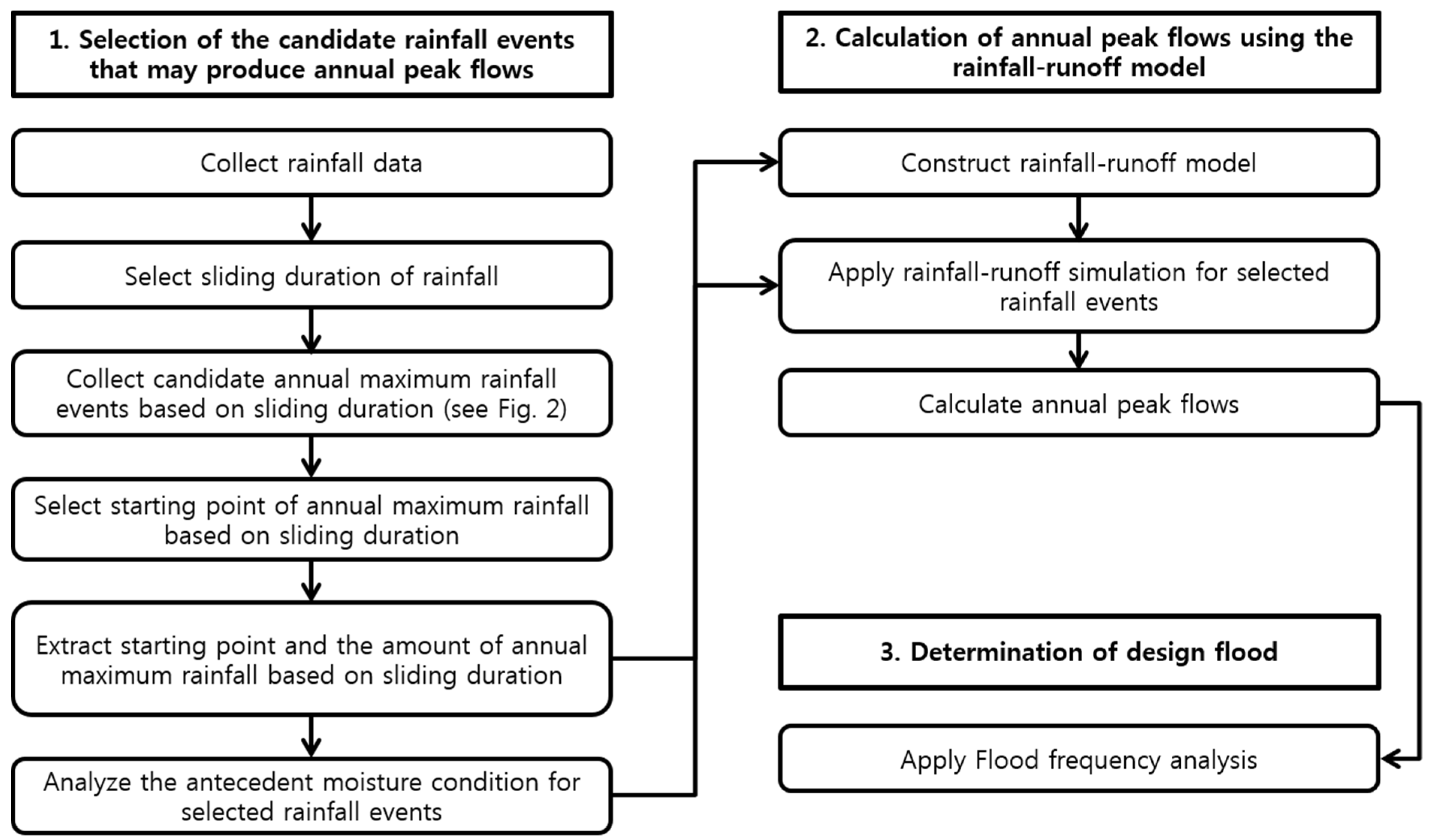
- (1)
- Select the candidate rainfall events which can produce the annual peak flows by analyzing time-series rainfall data and considering time step order and sliding duration;
- (2)
- Simulate the annual peak flows of the selected candidate rainfall events using the event-based model; and
- (3)
- Apply frequency analysis for the simulated annual peak flows (FASAP) from step 2.
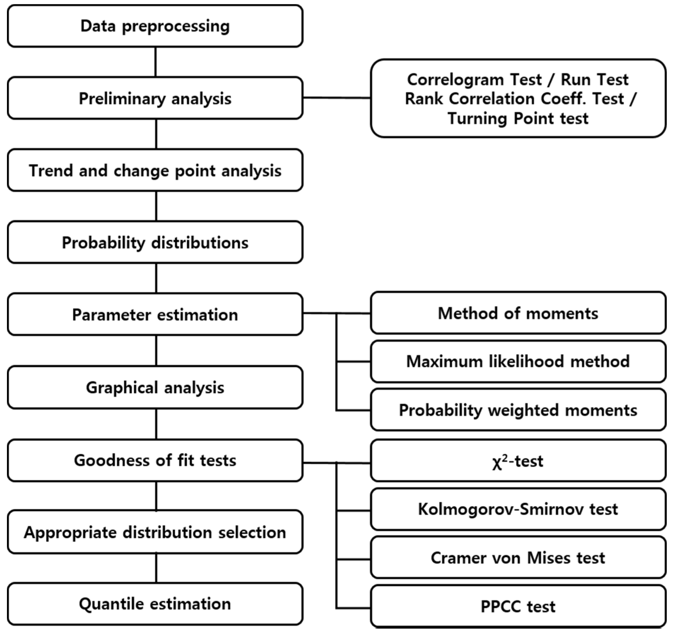
2. Research Method

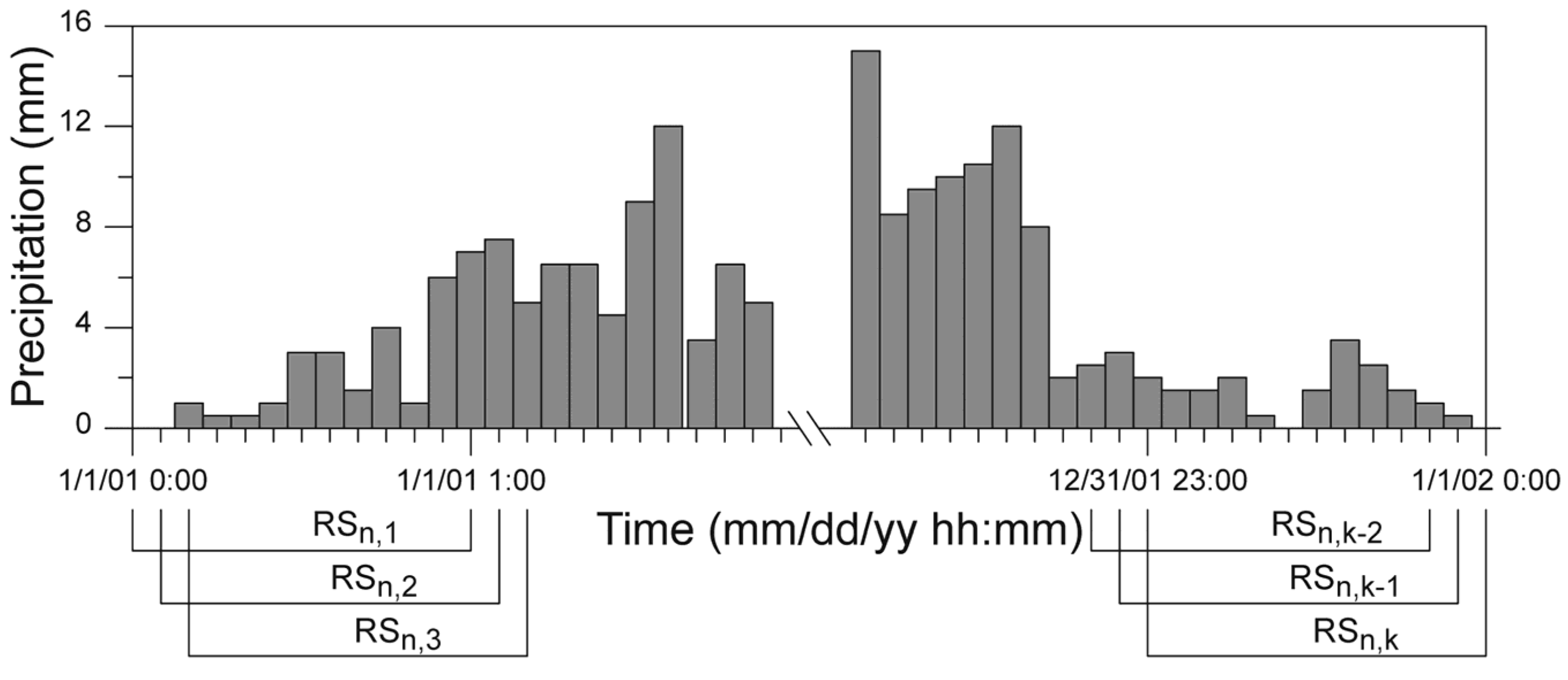
2.1. Sliding Maxima
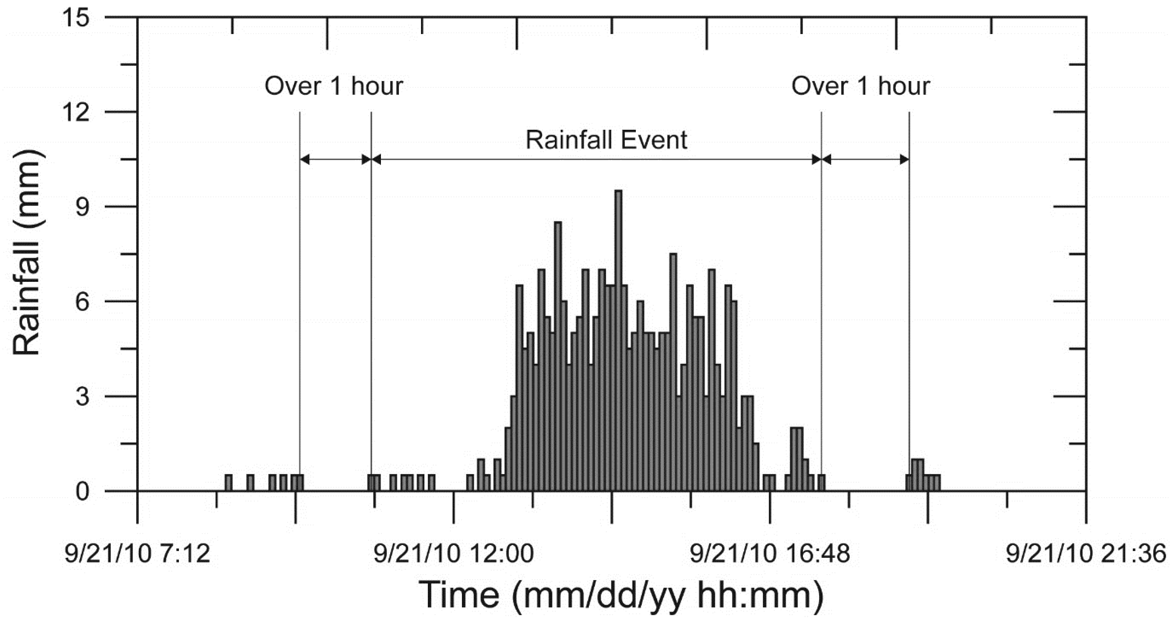
2.2. Identifying Independent Rainfall Events
2.3. Event-Based Simulation
2.4. Frequency Analysis

3. Application
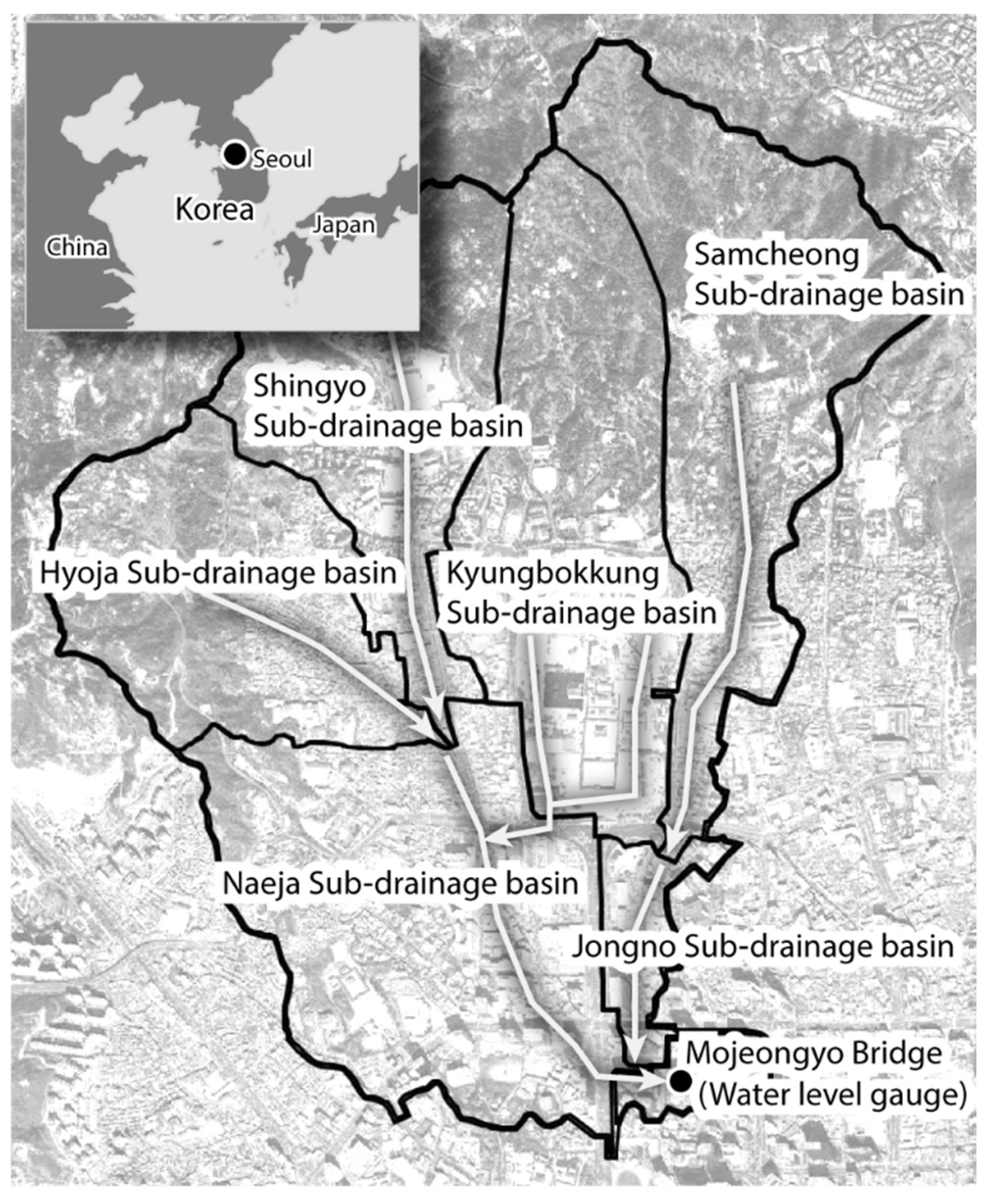
3.1. Watershed Description

| Drainage Basin | Sub-Drainage Basin | Area (ha) | Sub-Drainage Basin | Area (ha) | ||
|---|---|---|---|---|---|---|
| Hyoja drainage basin | Baegundong | Naeja | 121.84 | Joonghakcheon | Kyungbokkung | 110.96 |
| Singyo | 85.75 | Samcheong | 114.42 | |||
| Hyoja | 81.14 | Jongno | 14.79 | |||
| Subtotal | 288.73 | Subtotal | 240.17 | |||
| Total | 528.90 | |||||
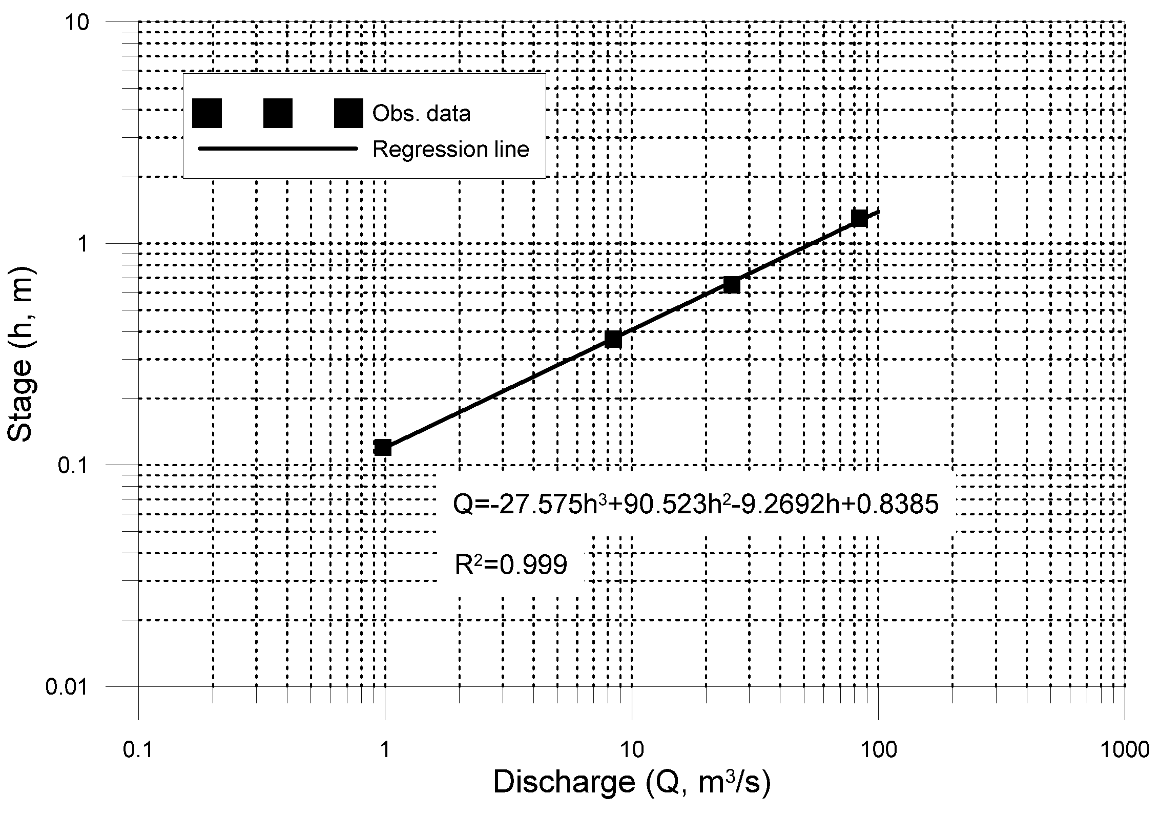
3.2. Composition of the Numerical Model
| Date | Stage (m) | Area Discharge Section (m2) | Average Velocity (m/s) | Discharge (m3/s) |
|---|---|---|---|---|
| 17 June 2010 | 0.12 | 4.27 | 0.23 | 0.98 |
| 27 August 2010 | 0.37 | 8.24 | 1.02 | 8.40 |
| 29 August 2010 | 0.65 | 12.68 | 2.01 | 25.49 |
| 21 September 2010 | 1.30 | 23.00 | 3.53 | 81.19 |
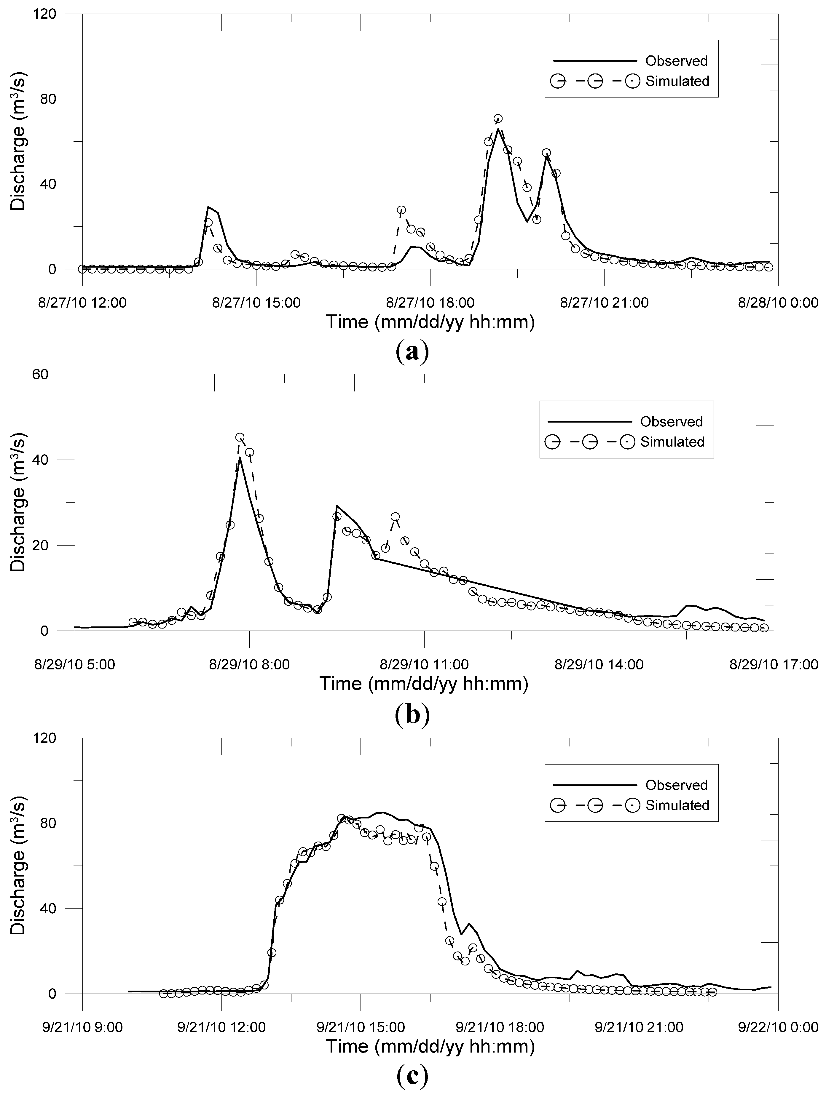
3.3. Model Calibration and Validation


3.4. Selecting Candidate Rainfall Events by Sliding Maxima Analysis
| No. of Years | Sliding Durations | No. of Events |
|---|---|---|
| 35 | 1-h, 2-h, 3-h | 35 |
| 6 | 1-h, 2-h | 6 |
| 3-h | 6 | |
| 8 | 1-h | 8 |
| 2-h, 3-h | 8 | |
| 1 | 1-h | 1 |
| 2-h | 1 | |
| 3-h | 1 | |
| Total | 66 | |
3.5. Determination of Independent Candidate Rainfall

| Duration Class (h) | No. of Events | Duration Class (h) | No. of Events |
|---|---|---|---|
| Under 2 | 2 | 6–12 | 25 |
| 2–3 | 7 | 12–24 | 10 |
| 3–6 | 18 | Over 24 | 4 |
| Total | 66 | ||
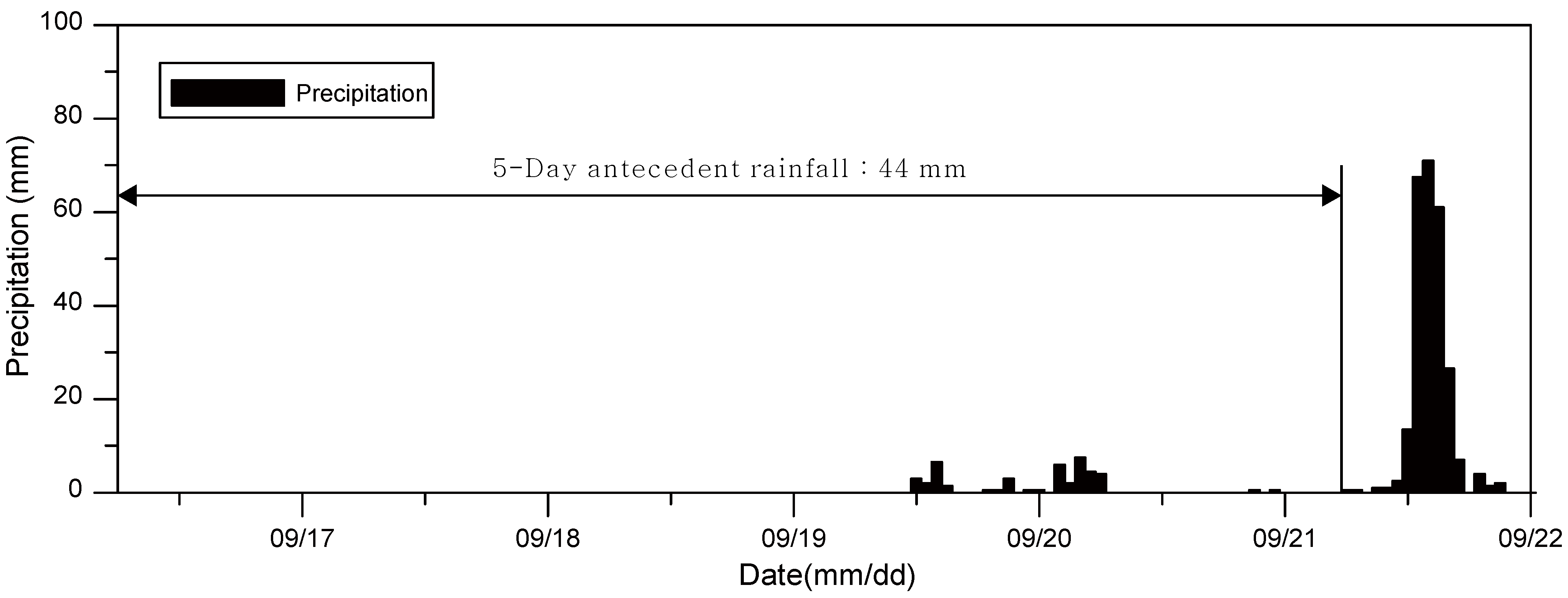
3.6. Determining Antecedent Moisture Conditions
| AMC Group | 5-Day Antecedent Rainfall, P5 (mm) | |
|---|---|---|
| Growing Season | Dormant Season | |
| I | P5 < 35.56 | P5 < 12.70 |
| II | 35.56 ≤ P5 < 53.34 | 12.70 ≤ P5 < 27.94 |
| III | P5 ≥ 53.34 | P5 ≥ 27.94 |

3.7. Determining Annual Peak Flows
| Year | Sliding Duration | Peak Flow (m3/s) | Year | Sliding Duration | Peak Flow (m3/s) | Year | Sliding Duration | Peak Flow (m3/s) |
|---|---|---|---|---|---|---|---|---|
| 1961 | 1-h, 2-h, 3-h | 37.7 | 1980 | 1-h | 33.3 | 1998 | 1-h | 72.7 |
| 1962 | 1-h, 2-h | 37.4 | 2-h, 3-h | 36.8 | 2-h, 3-h | 71.9 | ||
| 3-h | 18.3 | 1981 | 1-h, 2-h | 23.8 | 1999 | 1-h, 2-h, 3-h | 62.7 | |
| 1963 | 1-h, 2-h, 3-h | 67.1 | 3-h | 41.3 | 2000 | 1-h, 2-h, 3-h | 65.3 | |
| 1964 | 1-h, 2-h, 3-h | 96.7 | 1982 | 1-h, 2-h, 3-h | 70.6 | 2001 | 1-h, 2-h, 3-h | 99.4 |
| 1965 | 1-h, 2-h, 3-h | 63.4 | 1983 | 1-h, 2-h, 3-h | 75.4 | 2002 | 1-h, 2-h, 3-h | 74.4 |
| 1966 | 1-h, 2-h, 3-h | 83.0 | 1984 | 1-h, 2-h, 3-h | 73.5 | 2003 | 1-h | 78.4 |
| 1967 | 1-h, 2-h, 3-h | 71.0 | 1985 | 1-h, 2-h, 3-h | 75.2 | 2-h, 3-h | 76.5 | |
| 1968 | 1-h, 2-h, 3-h | 68.2 | 1986 | 1-h | 51.0 | 2004 | 1-h | 62.5 |
| 1969 | 1-h, 2-h, 3-h | 66.8 | 2-h, 3-h | 55.8 | 2-h | 31.3 | ||
| 1970 | 1-h, 2-h, 3-h | 64.5 | 1987 | 1-h, 2-h, 3-h | 82.1 | 3-h | 38.2 | |
| 1971 | 1-h, 2-h, 3-h | 81.0 | 1988 | 1-h, 2-h, 3-h | 47.8 | 2005 | 1-h, 2-h | 69.0 |
| 1972 | 1-h, 2-h, 3-h | 72.1 | 1989 | 1-h, 2-h, 3-h | 46.5 | 3-h | 65.3 | |
| 1973 | 1-h, 2-h, 3-h | 21.1 | 1990 | 1-h | 53.7 | 2006 | 1-h | 61.0 |
| 1974 | 1-h | 53.1 | 2-h, 3-h | 46.5 | 2-h, 3-h | 67.6 | ||
| 2-h, 3-h | 46.3 | 1991 | 1-h, 2-h, 3-h | 65.3 | 2007 | 1-h, 2-h | 48.5 | |
| 1975 | 1-h, 2-h, 3-h | 63.1 | 1992 | 1-h, 2-h, 3-h | 74.7 | 3-h | 24.3 | |
| 1976 | 1-h, 2-h | 62.0 | 1993 | 1-h, 2-h, 3-h | 72.5 | 2008 | 1-h, 2-h | 54.6 |
| 3-h | 46.3 | 1994 | 1-h, 2-h, 3-h | 37.8 | 3-h | 53.1 | ||
| 1977 | 1-h, 2-h, 3-h | 60.6 | 1995 | 1-h, 2-h, 3-h | 52.6 | 2009 | 1-h | 64.5 |
| 1978 | 1-h, 2-h, 3-h | 41.3 | 1996 | 1-h, 2-h, 3-h | 67.2 | 2-h, 3-h | 62.1 | |
| 1979 | 1-h, 2-h, 3-h | 52.1 | 1997 | 1-h, 2-h, 3-h | 49.0 | 2010 | 1-h, 2-h, 3-h | 83.3 |
3.8. Flood Frequency Analysis
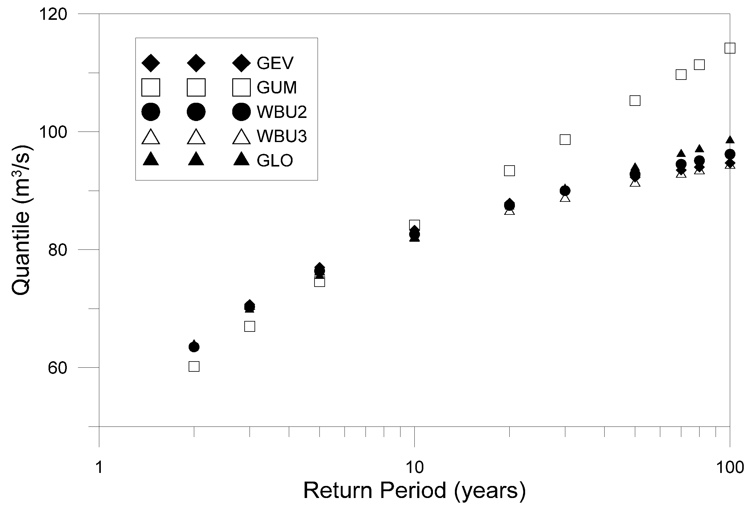
| Goodness of Fit Test | Probability Distribution | ||||
|---|---|---|---|---|---|
| GEV | GUM | WBU2 | WBU3 | GLO | |
| χ2 | O | X | O | O | O |
| Kolmogorov-Smirnov | O | O | O | O | O |
| Cramer von Mises | O | O | O | O | O |
| PPCC | O | X | O | O | O |
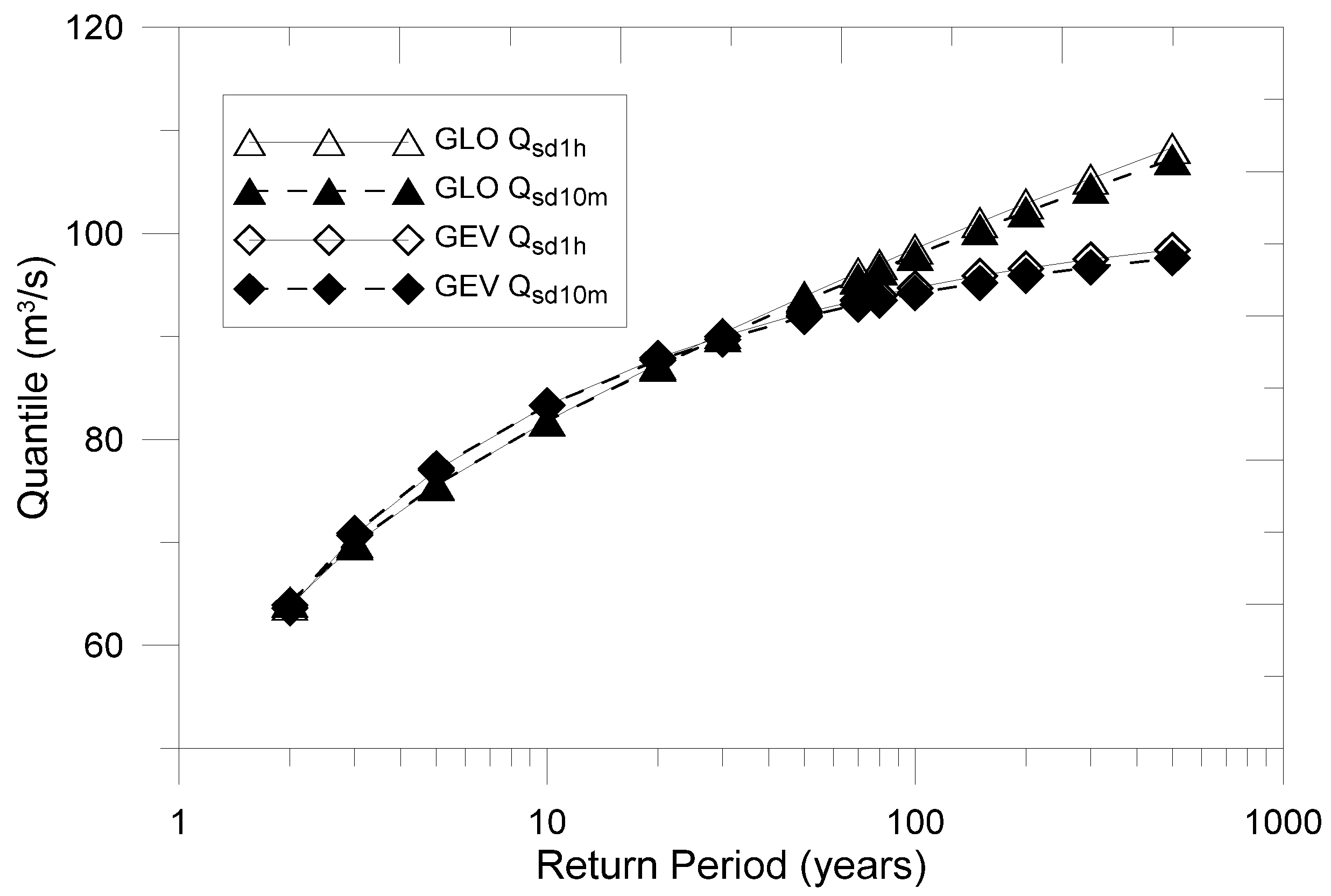
4. Sensitivity Analysis
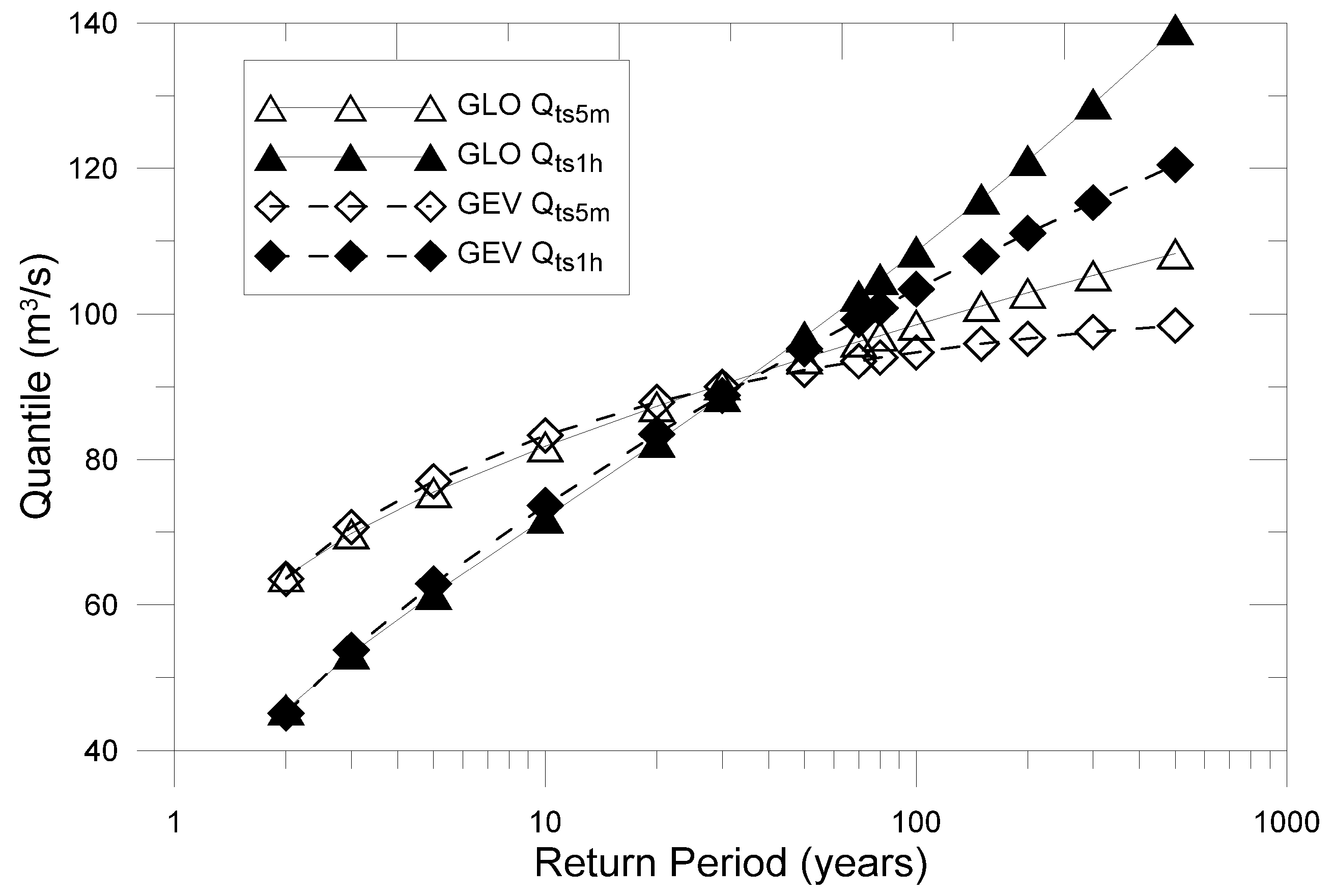
4.1. Time Step Order
| Return Period (Year) | GLO | GEV | ||||
|---|---|---|---|---|---|---|
| Qts5m (m3/s) | Qts1h (m3/s) | Difference | Qts5m (m3/s) | Qts1h (m3/s) | Difference | |
| 2 | 63.9 | 45.6 | −28.64% | 63.6 | 45.1 | −29.09% |
| 3 | 69.8 | 53.3 | −23.64% | 70.7 | 53.8 | −23.90% |
| 5 | 75.5 | 61.5 | −18.54% | 77.0 | 62.9 | −18.31% |
| 10 | 81.8 | 72.0 | −11.98% | 83.3 | 73.7 | −11.52% |
| 20 | 87.3 | 82.4 | −5.61% | 87.9 | 83.5 | −5.01% |
| 30 | 90.3 | 88.7 | −1.77% | 90.0 | 88.8 | −1.33% |
| 50 | 93.9 | 96.9 | 3.19% | 92.3 | 95.2 | 3.14% |
| 70 | 96.2 | 102.5 | 6.55% | 93.5 | 99.2 | 6.10% |
| 80 | 97.0 | 104.8 | 8.04% | 94.0 | 100.8 | 7.23% |
| 100 | 98.5 | 108.6 | 10.25% | 94.7 | 103.4 | 9.19% |
| 150 | 101.1 | 115.8 | 14.54% | 95.9 | 107.9 | 12.51% |
| 200 | 102.9 | 121.1 | 17.69% | 96.6 | 111.1 | 15.01% |
| 300 | 105.3 | 128.9 | 22.41% | 97.5 | 115.3 | 18.26% |
| 500 | 108.3 | 139.1 | 28.44% | 98.4 | 120.5 | 22.46% |

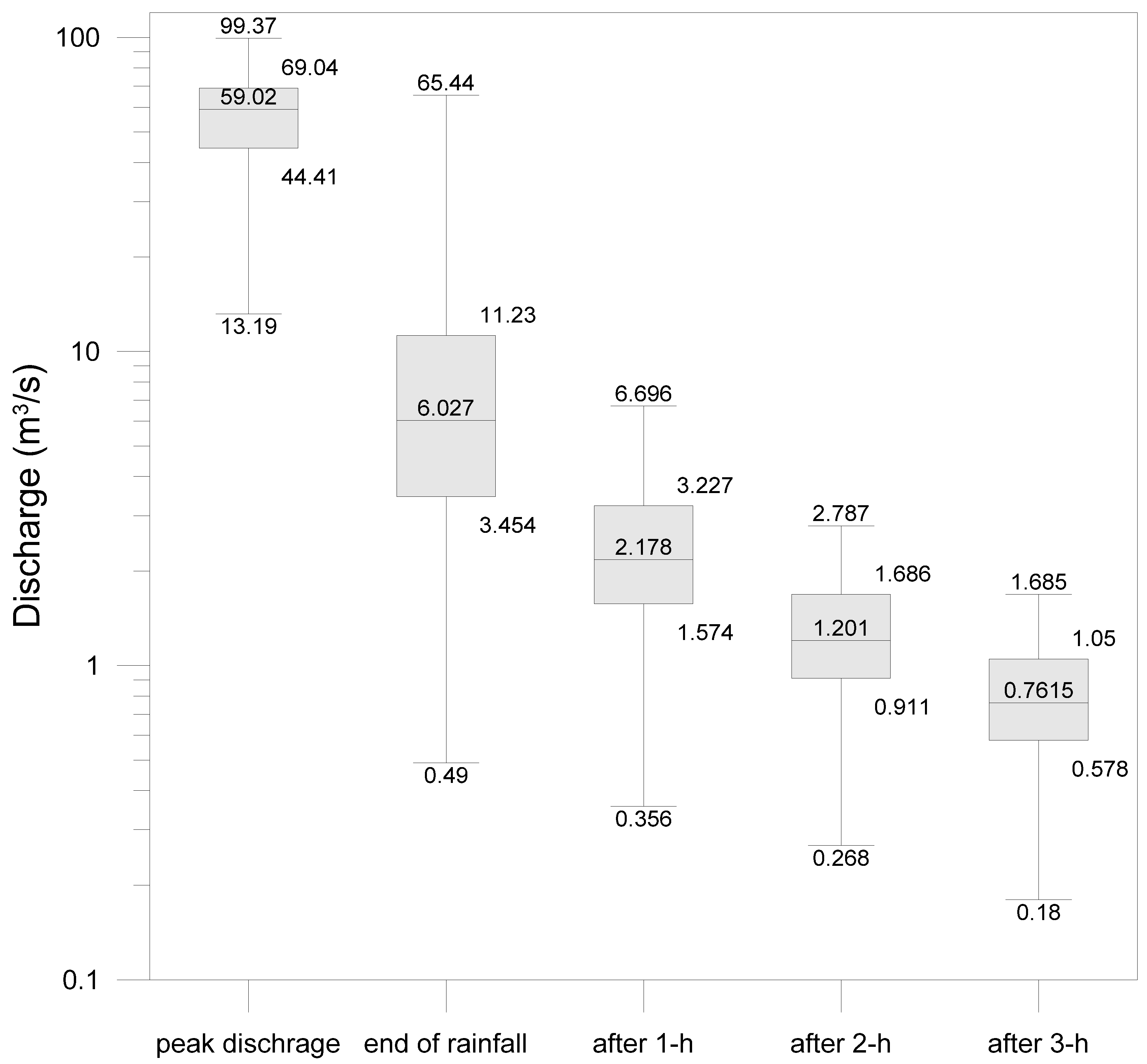
4.2. Sliding Duration
5. Comparative Analysis
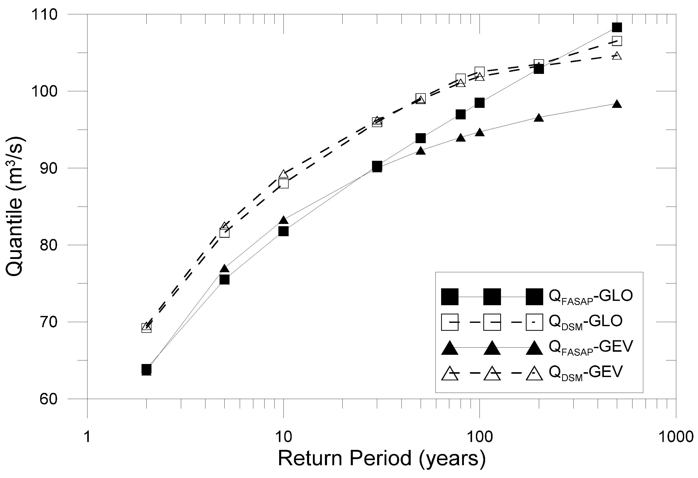
5.1. Design Storm Method
| Return Period (Year) | GEV (m3/s) | GLO (m3/s) | ||||
|---|---|---|---|---|---|---|
| DSM | FASAP | Difference | DSM | FASAP | Difference | |
| 2 | 69.5 | 63.6 | 9.26% | 69.2 | 63.9 | 8.30% |
| 5 | 82.5 | 77.0 | 7.17% | 81.6 | 75.5 | 8.08% |
| 10 | 89.3 | 83.3 | 7.21% | 88.0 | 81.8 | 7.59% |
| 30 | 96.2 | 90.0 | 6.94% | 96.0 | 90.3 | 6.29% |
| 50 | 98.9 | 92.3 | 7.14% | 99.1 | 93.9 | 5.53% |
| 80 | 101.1 | 94.0 | 7.55% | 101.6 | 97.0 | 4.78% |
| 100 | 101.9 | 94.7 | 7.62% | 102.5 | 98.5 | 4.09% |
| 200 | 103.3 | 96.6 | 6.91% | 103.5 | 102.9 | 0.59% |
| 500 | 104.7 | 98.4 | 6.36% | 106.5 | 108.3 | −1.63% |

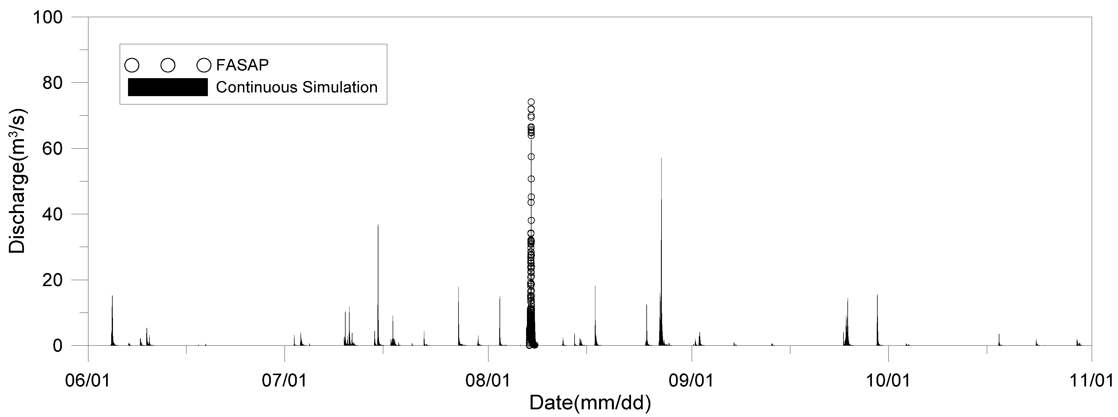
5.2. Continuous Simulation

| Year | Continuous Simulation | FASAP | Year | Continuous Simulation | FASAP | ||||
|---|---|---|---|---|---|---|---|---|---|
| Peak Flow | Peak Time | Peak Flow | Peak Time | Peak Flow | Peak Time | Peak Flow | Peak Time | ||
| 1961 | 26.8 | 07–14 05:04 | 37.7 | 07–14 04:45 | 1986 | 54.5 | 07–24 05:00 | 55.8 | 07–24 04:32 |
| 1962 | 19.6 | 08–08 09:59 | 37.4 | 08–05 10:10 | 1987 | 72.1 | 07–27 04:00 | 82.1 | 07–27 04:13 |
| 1963 | 55.0 | 07–17 10:00 | 67.1 | 08–14 04:34 | 1988 | 24.0 | 07–09 08:00 | 47.8 | 07–09 08:02 |
| 1964 | 92.8 | 09–13 03:00 | 96.7 | 09–13 02:51 | 1989 | 38.0 | 08–11 20:00 | 46.5 | 08–11 19:47 |
| 1965 | 61.4 | 07–20 05:54 | 63.4 | 07–20 05:54 | 1990 | 36.9 | 09–11 08:00 | 53.7 | 09–11 08:17 |
| 1966 | 79.7 | 07–15 16:00 | 83.0 | 07–15 16:15 | 1991 | 58.5 | 07–25 17:49 | 65.3 | 07–25 17:57 |
| 1967 | 57.4 | 08–25 18:00 | 71.0 | 08–25 18:19 | 1992 | 64.9 | 08–07 12:54 | 74.7 | 08–07 12:31 |
| 1968 | 68.1 | 07–04 01:00 | 68.2 | 07–04 00:15 | 1993 | 64.0 | 07–11 14:00 | 72.5 | 07–11 13:27 |
| 1969 | 57.7 | 09–19 12:05 | 66.8 | 09–19 12:35 | 1994 | 32.5 | 07–05 09:00 | 37.8 | 07–05 09:06 |
| 1970 | 57.1 | 06–25 12:50 | 64.5 | 06–25 12:06 | 1995 | 52.5 | 08–19 17:05 | 52.6 | 07–10 04:22 |
| 1971 | 66.7 | 07–17 06:00 | 81.0 | 07–17 04:40 | 1996 | 56.3 | 07–26 15:00 | 67.2 | 07–26 15:05 |
| 1972 | 62.2 | 08–19 11:00 | 72.1 | 08–19 10:18 | 1997 | 36.1 | 07–01 08:00 | 49.0 | 07–01 07:35 |
| 1973 | 14.6 | 08–17 17:00 | 21.1 | 07–30 00:58 | 1998 | 69.9 | 08–08 03:59 | 72.7 | 08–08 03:55 |
| 1974 | 35.9 | 08–03 05:00 | 53.1 | 07–29 14:17 | 1999 | 55.2 | 08–02 09:25 | 62.7 | 08–02 08:46 |
| 1975 | 40.6 | 07–25 09:00 | 63.1 | 07–25 08:17 | 2000 | 58.2 | 08–28 03:00 | 65.3 | 08–28 02:51 |
| 1976 | 54.5 | 08–13 18:59 | 62.0 | 08–13 19:01 | 2001 | 90.2 | 07–15 03:00 | 99.4 | 07–15 03:09 |
| 1977 | 33.3 | 07–04 04:05 | 60.6 | 07–04 04:47 | 2002 | 65.9 | 08–07 05:00 | 74.4 | 08–07 04:35 |
| 1978 | 29.9 | 06–25 16:00 | 41.3 | 06–25 21:19 | 2003 | 69.3 | 08–24 20:00 | 78.4 | 08–24 20:01 |
| 1979 | 31.0 | 08–02 12:00 | 52.1 | 08–02 09:24 | 2004 | 50.3 | 07–06 19:05 | 62.5 | 07–06 18:36 |
| 1980 | 22.4 | 07–14 05:04 | 36.8 | 07–14 05:52 | 2005 | 61.2 | 06–26 22:00 | 69.0 | 07–28 03:46 |
| 1981 | 31.8 | 07–12 08:00 | 41.3 | 07–01 21:26 | 2006 | 59.5 | 07–12 10:00 | 67.6 | 07–16 00:56 |
| 1982 | 54.4 | 07–27 02:00 | 70.6 | 07–27 02:06 | 2007 | 24.9 | 08–04 12:00 | 48.5 | 08–04 11:54 |
| 1983 | 69.6 | 09–02 06:00 | 75.4 | 09–02 05:16 | 2008 | 35.2 | 06–02 20:00 | 54.6 | 07–24 05:04 |
| 1984 | 64.9 | 09–01 06:54 | 73.5 | 09–01 06:17 | 2009 | 57.5 | 07–09 14:00 | 62.1 | 07–09 14:17 |
| 1985 | 64.9 | 08–16 17:00 | 75.2 | 08–16 16:41 | 2010 | 81.6 | 09–21 15:05 | 83.3 | 09–21 14:42 |
6. Conclusions
- (1)
- To extract and separate the rainfall events the MIT was initially set to 1 h. After applying the studied urban watershed, the remaining runoff was maintained at less than 1 m3/s after 3 h from the end of rainfall. Thus, setting the MIT to 3 h was determined as the rule for candidate rainfall event separation.
- (2)
- The estimated flood quantiles based on the time step orders of 5 min and 1 h showed that the differences between these time steps was between −29.09% and +28.44%. Estimating appropriate flood quantiles with the time step order of 1 h was not possible in a small urban watershed with a quick hydrologic response, which is the time step usually used in the continuous simulation method.
- (3)
- To review the appropriate sliding duration, sliding durations of 1-h, 2-h, and 3-h were tested, and the results from comparing the flood quantiles estimated by setting the sliding duration and time interval at 10 min showed less than 1% differences between the GEV and GLO distributions. Setting the sliding duration and time interval at 1 h was appropriate for a small urban watershed.
- (4)
- The estimated flood quantiles from the proposed FASAP method were approximately 10% smaller than those quantiles from the conventional design storm method for the GEV distribution. This result is consistent with existing research results that compare the flood quantiles using statistical approach, the design storm method, and the continuous simulation method.
- (5)
- The peak times of FASAP were in good agreement with those obtained by continuous simulation. This is a results of comparison between continuous simulation with 1 h time step and FASAP with 5 min time step. If they had a same level of 5 min time step order the accordance rate would be expected to be higher than this results. However, the results indicate that FASAP could find the time when annual maximum peak flows were occurred successfully and could be regarded as an appropriate method to estimate design flood.
Acknowledgments
Author Contributions
Conflicts of Interest
References
- Stedinger, J.R.; Griffis, V.W. Flood frequency analysis in the United States: Time to update. J. Hydrol. Eng. 2012, 13, 199–204. [Google Scholar] [CrossRef]
- Rogger, M.; Kohl, B.; Pirkl, H.; Viglione, A.; Komma, J.; Kirnbauer, R.; Merz, R.; Blöschl, G. Runoff models and flood frequency statistics for design flood estimation in Austria—Do they tell a consistent story? J. Hydrol. 2012, 456–457, 30–43. [Google Scholar] [CrossRef]
- Hydrology Handbook; American Society of Civil Engineers Publications: Reston, VA, USA, 1996.
- Katz, R.W.; Parlange, M.B.; Naveau, P. Statistics of extremes in hydrology. Adv. Water Resour. 2002, 25, 1287–1304. [Google Scholar] [CrossRef]
- Klemes, V. Probability of Extreme Hydrometeorological Events—A Different Approach. In Extreme Hydrological Events: Precipitation, Floods and Droughts; Kundzewicz, Z.W., Rosbjerg, D., Simonovic, S.P., Takeuchi, K., Eds.; International Association of Hydrological Sciences: Wallingford, UK, 1993; pp. 167–176. [Google Scholar]
- Beighley, R.E.; Moglen, G.E. Adjusting measured peak discharges from an urbanizing watershed to reflect a stationary land use signal. Water Resour. Res. 2003, 39. [Google Scholar] [CrossRef]
- Archer, D.R.; Climent-Soler, D.; Holman, I.P. Changes in discharge rise and fall rates applied to impact assessment of catchment land use. Hydrol. Res. 2010, 41, 13–26. [Google Scholar] [CrossRef]
- O’Connell, E.; Ewen, J.; O’Donnell, G.; Quinn, P. Is there a link between agricultural land-use management and flooding? Hydrol. Earth Syst. Sci. 2007, 11, 96–107. [Google Scholar] [CrossRef]
- Beven, K.; Young, P.; Romanowicz, R.; O’Connell, E.; Ewen, J.; O’Donnell, G.; Holman, I.; Morris, J.; Hollis, J.; Rose, S.; et al. Analysis of Historical Data Sets to Look for Impacts of Land Use and Management Change on Flood Generation; Department for Environment Food and Rural Affairs: London, UK, 2007.
- Halcrow Group Limited. Delivery of Making Space for Water: The Role of Land Use and Land Management in Delivering Flood Risk Management; Environment Agency: Rotherham, UK, 2008.
- Alfieri, L.; Laio, F.; Claps, P. A simulation experiment for optimal design hyetograph selection. Hydrol. Process. 2008, 22, 813–820. [Google Scholar] [CrossRef]
- Grimaldi, S.; Petroselli, A.; Serinaldi, F. Design hydrograph estimation in small and ungauged watersheds: Continuous simulation method versus event-based approach. Hydrol. Process. 2012, 26, 3124–3134. [Google Scholar] [CrossRef]
- Rahman, A.; Hoang, T.M.T.; Weinmann, P.E.; Laurenson, E.M. Joint Probability Approaches to Design Flood Estimation: A Review; Cooperative Research Center for Catchment Hydrology, Monash University: Clayton, Australia, 1998. [Google Scholar]
- Guo, Y.; Markus, M. Analytical probabilistic approach for estimating design flood peaks of small watersheds. J. Hydrol. Eng. 2011, 16, 847–857. [Google Scholar] [CrossRef]
- Adams, B.J.; Howard, C.D.D. Design storm pathology. Can. Water Resour. J. 1986, 11, 49–55. [Google Scholar] [CrossRef]
- Guo, Y. Hydrologic design of urban flood control detention ponds. J. Hydrol. Eng. 2001, 6, 472–479. [Google Scholar] [CrossRef]
- Marsalek, J.; Watt, W.E. Design storms for urban drainage design. Can. J. Civ. Eng. 1984, 11, 574–584. [Google Scholar] [CrossRef]
- Packman, J.C.; Kidd, C.H.R. A logical approach to the design storm concept. Water Resour. Res. 1980, 16, 994–1000. [Google Scholar] [CrossRef]
- Boughton, W.; Droop, O. Continuous simulation for design flood estimation—A review. Environ. Model. Softw. 2003, 18, 309–318. [Google Scholar] [CrossRef]
- Boughton, W. The Australian water balance model. Environ. Model. Softw. 2004, 19, 943–956. [Google Scholar] [CrossRef]
- Chetty, K.; Smithers, J. Continuous simulation modeling for design flood estimation in South Africa: Preliminary investigations in the Thukela catchment. Phys. Chem. Earth 2005, 30, 634–638. [Google Scholar] [CrossRef]
- Viviroli, D.; Zappa, M.; Schwanbeck, J.; Gurtz, J.; Weingartner, R. Continuous simulation for flood estimation in ungauged mesoscale catchments of Switzerland—Part I: Modeling framework and calibration results. J. Hydrol. 2009, 377, 191–207. [Google Scholar] [CrossRef]
- Osborn, H.B.; Lane, L. Precipitation-runoff relations for very small semiarid rangeland watersheds. Water Resour. Res. 1969, 5, 419–425. [Google Scholar] [CrossRef]
- Van Montfort, M.A.J. Sliding maxima. J. Hydrol. 1990, 118, 77–85. [Google Scholar] [CrossRef]
- Dunkerley, D. Identifying individual rain events from pluviograph records: A review with analysis of data from an Australian dryland site. Hydrol. Process. 2008, 22, 5024–5036. [Google Scholar] [CrossRef]
- Fisher, J.S.; Grayman, W.M.; Eagleson, P.S. Evaluation of Radar and Raingage Systems for Flood Forecasting; Department of Civil Engineering, Massachusetts Institute of Technology: Cambridge, MA, USA, 1971. [Google Scholar]
- Todorovic, P.; Yevjevich, V. Stochastic Processes of Precipitation; Colorado State University: Fort Collins, CO, USA, 1969. [Google Scholar]
- FARD User Manual; National Disaster Management Institute: Seoul, Korea, 2006.
- Technical Description: XPSWMM; XP Solutions Inc.: Queensland, Australia, 2011.
- Environmental Geo-Information System. Available online: http://egis.me.go.kr/main.do (accessed on 10 May 2014).
- Korean Soil Information System. Available online: http://soil.rda.go.kr/eng/index.jsp (accessed on 10 May 2014).
- Natural Resources Conservation Service (NRCS). Urban Hydrology for Small Watersheds; Technical Release No. 55; U.S. Department of Agriculture: Washington, DC, USA, 1986.
- Flood Estimation Handbook; Institute of Hydrology: Wallingford, UK, 1999.
- Design Flood Estimation Tips; Ministry of Land, Transport and Maritime Affairs (MoLIT): Seoul, Korea, 2012.
- Boughton, W.C.; Hill, P. A Design Flood Estimation System Using Data Generation and a Daily Water Balance Model; Report 97/8 in CRC for Catchment Hydrology; Monash University: Melbourne, Australia, 1997. [Google Scholar]
- Calver, A.; Stewart, E.; Goodsell, G. Comparative analysis of statistical and catchment modeling approaches to river flood frequency estimation. J. Flood Risk Manag. 2009, 2, 24–31. [Google Scholar] [CrossRef]
- McKerchar, A.I.; Macky, G.H. Comparison of a regional method for estimating design floods with two rainfall-based methods. J Hydrol. N. Z. 2001, 40, 129–138. [Google Scholar]
© 2014 by the authors; licensee MDPI, Basel, Switzerland. This article is an open access article distributed under the terms and conditions of the Creative Commons Attribution license (http://creativecommons.org/licenses/by/4.0/).
Share and Cite
Ahn, J.; Cho, W.; Kim, T.; Shin, H.; Heo, J.-H. Flood Frequency Analysis for the Annual Peak Flows Simulated by an Event-Based Rainfall-Runoff Model in an Urban Drainage Basin. Water 2014, 6, 3841-3863. https://doi.org/10.3390/w6123841
Ahn J, Cho W, Kim T, Shin H, Heo J-H. Flood Frequency Analysis for the Annual Peak Flows Simulated by an Event-Based Rainfall-Runoff Model in an Urban Drainage Basin. Water. 2014; 6(12):3841-3863. https://doi.org/10.3390/w6123841
Chicago/Turabian StyleAhn, Jeonghwan, Woncheol Cho, Taereem Kim, Hongjoon Shin, and Jun-Haeng Heo. 2014. "Flood Frequency Analysis for the Annual Peak Flows Simulated by an Event-Based Rainfall-Runoff Model in an Urban Drainage Basin" Water 6, no. 12: 3841-3863. https://doi.org/10.3390/w6123841
APA StyleAhn, J., Cho, W., Kim, T., Shin, H., & Heo, J.-H. (2014). Flood Frequency Analysis for the Annual Peak Flows Simulated by an Event-Based Rainfall-Runoff Model in an Urban Drainage Basin. Water, 6(12), 3841-3863. https://doi.org/10.3390/w6123841