Effects of Soil and Water Conservation Measures on Groundwater Levels and Recharge

Abstract

Measures of soil and water conservation (SWC) could affect the hydrological process. The impacts of typical measures on groundwater recharge, levels and flow were analyzed based on simulated rainfall experiments and a groundwater model. The three-dimensional finite-difference groundwater flow model (MODFLOW) was calibrated and verified for bare slope, grassland and straw mulching scenarios based on the experiments. The results of the verification in groundwater balance, levels, runoff and flow field all showed that MODFLOW could be applied to study the impact of SWC measures on groundwater. Meanwhile, the results showed the recharge rate (α) and specific yield of the three soil layers (Sy1, Sy2 and Sy3) were the most sensitive parameters to the change in the underlying surface. Then, the impacts of the SWC measures’ construction and destruction on the groundwater regime were studied. The results indicated the measures could strengthen groundwater recharge. The amounts of groundwater recharge, runoff and level were on the order of straw mulching > grassland > bare slope. When the underlying surface was converted from grass and mulching to bare slope, the recharge decreased by 42.2% and 39.1%. It was concluded that SWC measure construction would increase groundwater recharge and the measure destruction would decrease recharge.

1. Introduction

It is well recognized that land cover and land use change have significant effects on hydrological processes such as evapotranspiration (ET), soil moisture and groundwater recharge [1,2]. Increasing or decreasing measures of soil and water conservation changes both the land cover and land use, which could alter the hydrologic cycle and affect the quantity of water that is available for runoff, streamflow and ground water flow.

For land-use change, groundwater research has mainly focused on the changes in water quality, thereby neglecting changes in its quantity [1,3,4,5]. The impacts of land-use changes on the quantity of groundwater have received considerable attention based on field observations. Zhang and Schilling [2] studied the effects of land cover on the water table, soil moisture, evapotranspiration, and groundwater recharge through water level measurements that were collected from two monitoring wells that were situated in the central portion of the Walnut Creek watershed at the Neal Smith National Wildlife Refuge in Jasper County, Iowa. Scanlon et al. [6] studied the impact of the conversion of natural rangeland ecosystems to agricultural ecosystems on groundwater recharge and quality through point and areal studies in the southwestern US. In Nigeria, Adekalu et al. [7] reported that mulching the soil surface with a layer of plant residue was an effective method of conserving water and soil because it reduced surface runoff, increased the infiltration of water into the soil and retarded soil erosion in the laboratory using a rainfall simulator. Adams [8] found that straw significantly increased the infiltration and movement of excess water in Temple, Texas. Increasing the soil cover with mulch decreased the runoff and soil loss and increased the apparent infiltration [8,9]. Vegetation also played a key role in the interactions between groundwater and surface-water systems, because of its direct and indirect influence on the recharge and the dependence of vegetation communities on groundwater [10]. The importance of vegetation cover in maintaining runoff and improving infiltrability is well known and has been discussed extensively [11,12,13,14]. Marston [15] reported that vegetation cover of 65% or more significantly reduced runoff and increased infiltration. Huang [11] simulated rainfall events to study the effects of various factors on the soil moisture increase after rainfall and found that vegetation cover yieldd a greater soil moisture increase than did bare land and was the most important factor in determining the recharge coefficient.

In the Kumamoto Plain of Japan, Moukana and Koike [16] constructed a spatial model of the actual temporal changes in groundwater levels as related to changes in the land-cover uses and specified the main factors influencing these changes. He and Wang et al. [17] used a distributed four-block three-layer water balance model to evaluate the effect of land use change on groundwater table fluctuation in the Dogo Plain of the Seto Inland Sea, Japan. Cho and Barone et al. [18] determined the impact of land development activities on the subsurface flow regime in the upper Roanoke River watershed using MODFLOW and found that decreases in both hydraulic head and streamflow coincided with increases in impervious land.

A monitoring approach may lead to more direct estimates of the impact of land development on subsurface flows, but it is expensive and time demanding [18]. Model building and simulation are becoming easier and faster through the implementation of advances in software and hardware [19]. Modeling is one of the most powerful techniques available for studying large and complex systems, but because monitoring data are not necessarily sufficient, the future state of the environment cannot be forecast from monitoring data [20]. However, models require good quality data on the physical (such as topography, land use, soils, canals, drainage ditches, climate and crops) and hydrogeological (aquifer system, boundary conditions and main hydraulic parameters) settings [21]. Models are efficient and credible only if the field measurement support evaluation of model parameters and provide data for calibration and verification or model credibility and interoperation.

We can see that land cover and land use change significantly affect hydrological processes. However, the study of the effects on groundwater has mostly concentrated on local variation in the water levels based on several monitoring wells, and the comprehensive impacts on the watershed have concentrated on surface runoff and soil infiltration. It is difficult to study the impact of soil and water conservation measures, especially a single measure, on the groundwater regime. Therefore, a mathematical model may be a better choice. Furthermore, the results from the indoor simulations were executed under very specific conditions and could not be compared directly with those from large-scale areas, making it difficult to transfer these results to the field quantitatively. However, because the rainfall simulation experiments were widely used in rainfall-runoff research, a monitoring approach may lead to more direct and comprehensive estimates. The results may be used to qualitatively study the changed laws in large-scale areas and will be helpful for improving the understanding of the effects on groundwater regime or it might provide an idea for studying it at least.

Therefore, linkage between experimental tools and modeling approaches to study the impact of soil and water conservation measures on the groundwater regime will be indispensable. The overall goal of this study is to investigate the impact of soil and water conservation measures on the groundwater levels and recharge observed in experiments on the laboratory scale and modeling experiments with MODFLOW. Meanwhile, a quantitative analysis could provide insight for studying a watershed scale to help decision-makers manage water resources.

2. Materials and Methods

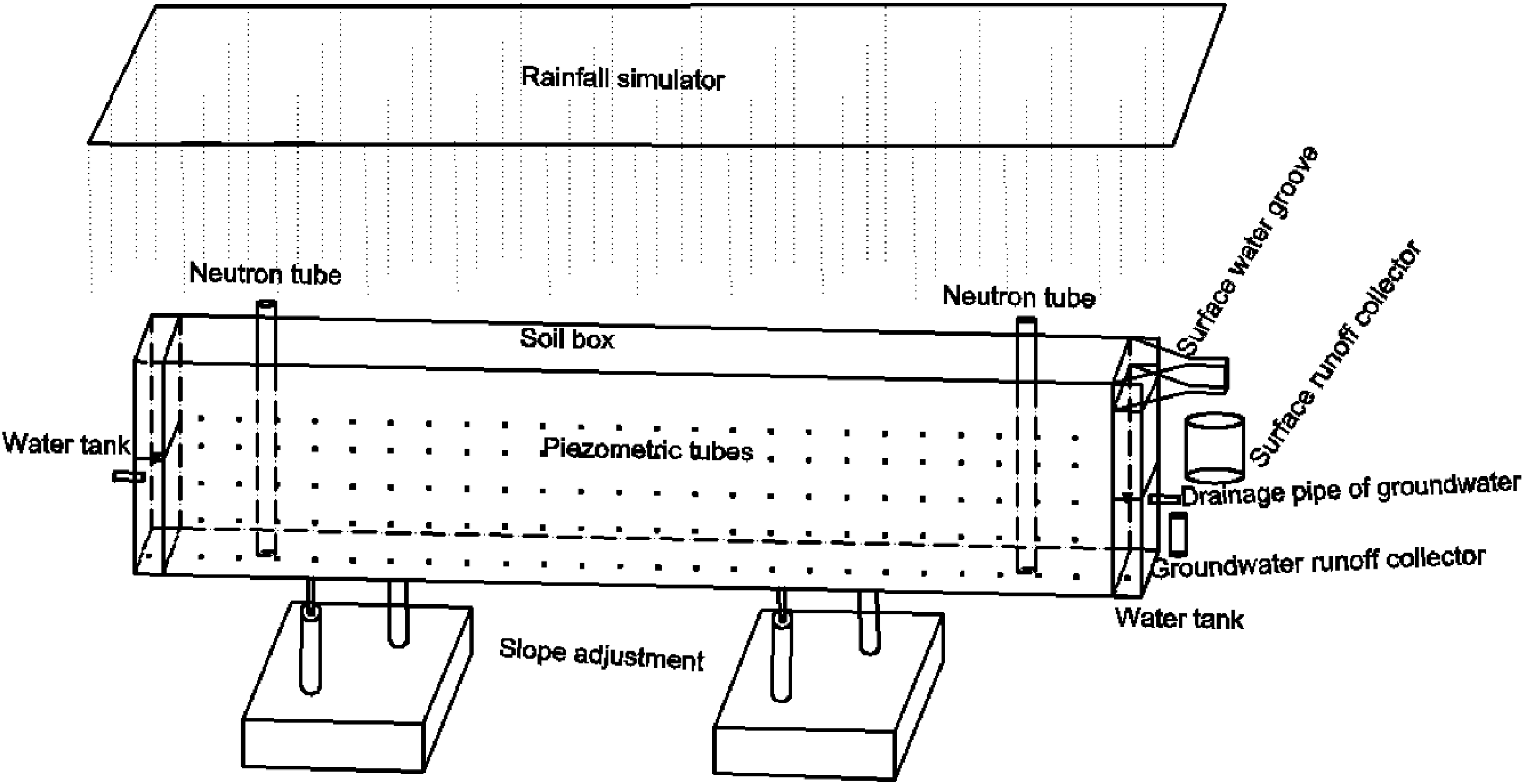
2.1. Experimental Conditions and Equipment of Simulated Rainfall Experiments

The simulated rainfall experiments were performed in the Rainfall Simulation Hall of the State Key Laboratory of Soil Erosion and Dryland Farming on the Loess Plateau of China in 2012. The simulated rainfall system, with an automatic simulation device for the under sprinkler, could ensure that the kinetic energy of the simulated precipitation is close to that of natural rainfall for the mean fall-height of 18 m [22]. The experiments were conducted in the sand-box model [23,24] as depicted in Figure 1. The soil flume size for lab experiments was length × width × depth = 5.3 m × 1 m × 1 m and was fitted with four wheels to facilitate transportation and a jack to allow the slope to be adjusted from 0° to 35°. There were two water tanks, 0.15 m × 1 m × 1 m, in front and back of the model for the regulation of the groundwater level. Above the front side of the water tank, there was one surface water groove and there was one drainage pipe of groundwater in the 0.39 m high at the front side of the water tank, and 120 sets of piezometric tubes, which row spacing was 0.2-m × 0.2-m, for level observation were installed on the left side of the sand-box model. Two tubes of neutron probe were installed to a depth of 0.9 m in the experimental flume for soil moisture control [22]. In this study, the flume was fixed at an angle of 3° because a Conversion of Cropland to Forest Project was implemented in bare slope with a gradient larger than 6° in 1998 in China. Therefore, a gradient of 3° was selected as the studying slope. Three water and soil conservation measures were considered, including bare slope scenario, grassland scenario and straw mulching scenario, such as in Figure 2. The first scenario was the bare slope. The second scenario was the straw mulching, which was designed as 0.4 kg straw /m², and its coverage was approximately 85%–90%. The third scenario was grassland, the grass species was Ophiopogon japonicus with coverage of 65%–70%, the planting structure was 10-cm row spacing × 5-cm plant spacing × 8.2-cm average plant height and the grass was planted outside 2 months before experiments and transplanted into flume.

Figure 1. The experimental flume.

Figure 1. The experimental flume.

Figure 2. Pictures of different soil and water conservation measures: (a) Bare Slope; (b) Grass Land; (c) Straw Mulching.

Figure 2. Pictures of different soil and water conservation measures: (a) Bare Slope; (b) Grass Land; (c) Straw Mulching.

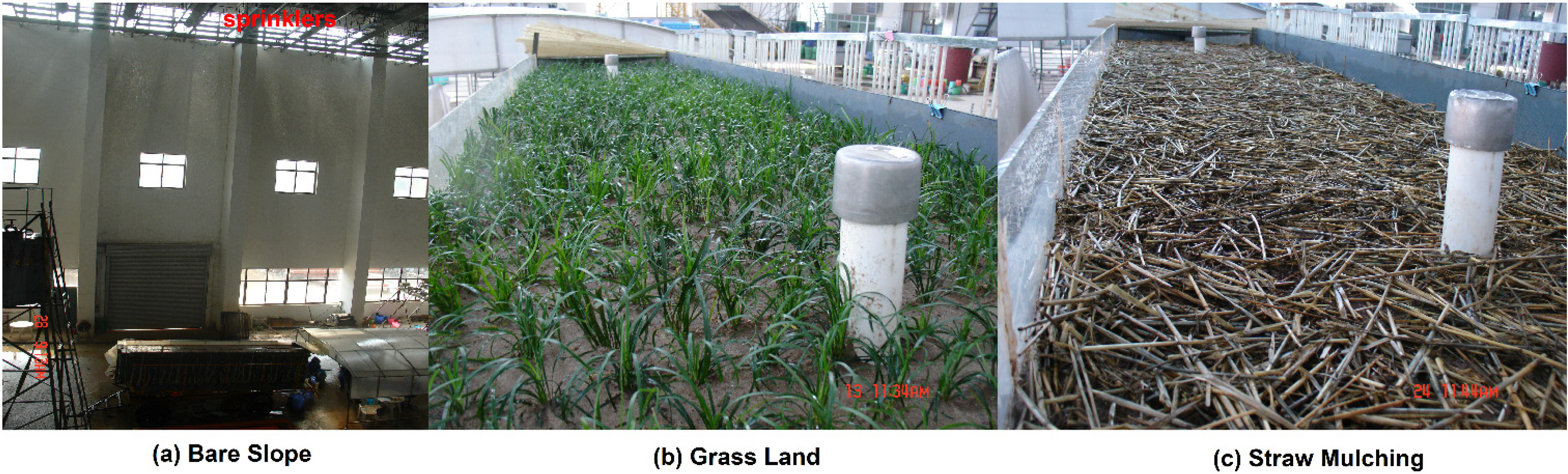
2.2. Experimental Materials and Monitoring Methods

The test materials included riversand and Lou soil. The riversand samples were dug from the middle and lower reaches of the Wei River bank in Yangling District, and the Lou soil was also collected from Yangling District, Shaanxi Province, China [22]. The samples were packed into the flume layer by layer. The experimental flume was divided into three layers, and the thicknesses of its layers were 0.5, 1 and 98.5 cm from top to bottom, respectively. The upper confining layer mostly consisted of clay, whereas the mixed soil comprised of Lou soil and fine sand. There were patches of riversand within the clay bed, making the bed act as a leaky confining layer. The second layer consisted of river sand with a particle size of less than 0.25 mm. The third layer consisted of medium sand and the soil bulk density was 1.4–1.5 g/cm³.

The main monitoring items that were measured during the experiments were as follows: the surface runoff amount, the surface runoff during the process, the groundwater runoff, the groundwater levels, the soil moisture [22]. The surface runoff was collected by collecting buckets for 30 s at 5-min intervals during the experiments. The groundwater runoff was collected by measuring cylinders per 2000 mL continuously for approximately 8 h. Then, the monitoring interval was lengthened gradually until the water level dropped to the initial control water level. The groundwater levels were recorded for every 10-min. The soil moisture was measured by the neutron probe method with Diviner 2000 before and after precipitation, and the temperatures of the surface and ground water were also recorded during each simulation.

2.3. MODFLOW

MODFLOW (Modular Three-dimensional Finite-difference Ground-water Flow Model) is a computer program that simulates three-dimensional ground-water flow through a porous medium by using a finite-difference method [25]. The three-dimensional movement of ground water of constant density through porous earth material may be described by the partial-differential equation [25]:

$$\frac{\partial }{\partial x}\left(Kxx-\frac{h}{x}\right)+\frac{\partial }{\partial y}\left(Kyy-\frac{h}{y}\right)+\frac{\partial }{\partial z}\left(Kzz-\frac{h}{z}\right)+W=Ss\frac{\partial h}{\partial t}$$

(1)

where Kxx, Kyy, and Kzz are values of hydraulic conductivity along the x, y, and z coordinate axes, which are assumed to be parallel to the major axes of hydraulic conductivity (m/s); h is the potentiometric head (m); W is the volumetric flux per unit volume representing sources and/or sinks of water, with W < 0 for the flow out of the ground water system, and W > 0 for the flow into the system; Ss is the specific storage of the porous material (1/m); and t is time (min).

A conceptual model of the soil flume was developed based on the hydrogeological information and simulated rainfall experimental observation. The study area was divided into 50 rows and 265 columns, and the cells were identical regular rectangles. Each cell size was 4 × 10⁻⁴ square meters. The entire model structure was a matrix of 50 rows × 265 columns × 3 layers. The model was divided into three aquifers with gradient of 3°. The thicknesses of the aquifers were 0.5, 1 and 98.5 cm from top to bottom. The edge of the model domain was modeled as a no-flow boundary. The actual quantities of groundwater abstraction from the drain pipe were treated as a flux boundary condition in the form of a pumping well. Groundwater recharge from rainfall was modeled as a recharge package in MODFLOW [22]. According to the actual condition of the rainfall experiments, the groundwater system could be described as a conceptual hydrologic model of three layers, homogeneous, horizontal isotropy, three-dimensional, and transient flow system. The initial conditions refer to the head distribution everywhere in the system at the beginning of the simulation and are thus boundary conditions in time [26]. The initial value and the range of hydraulic conductivity and storage coefficient values at different layers were assigned to each active grid cell by the interpolation of discrete property data that were derived from water releasing test analysis and regional geology data. Combining the initial and boundary conditions, the numeric model was constructed [27].

To evaluate the performance of the calibration and validation of the MODFLOW, six statistical indicators were used, including the residual mean (RM), absolute residual mean (ARM), standard error of the estimate (SEE), root mean squared error (RMS), normalized root mean squared (NRMS) and correlation coefficient (Cor).

3. Results and Discussion

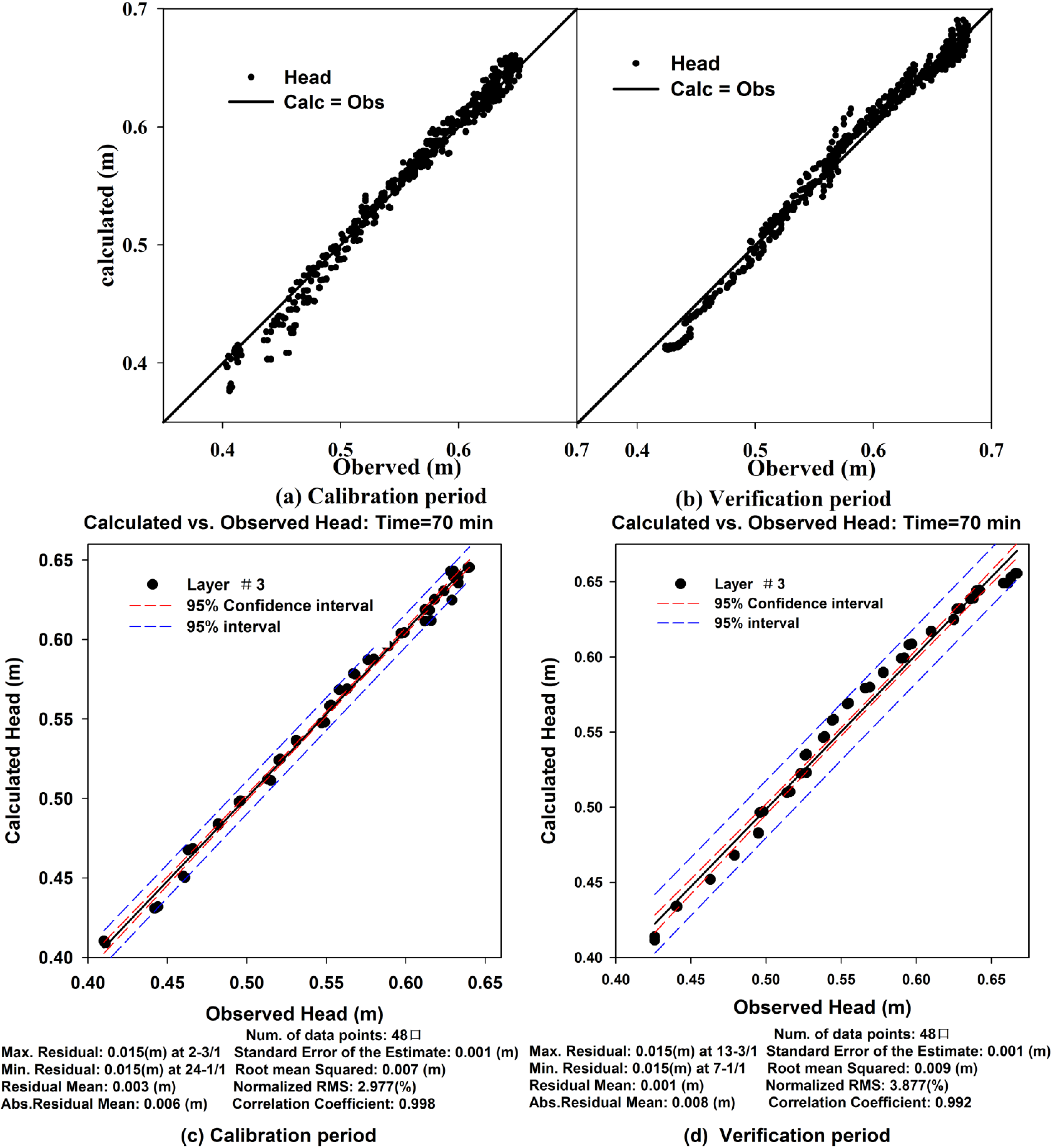
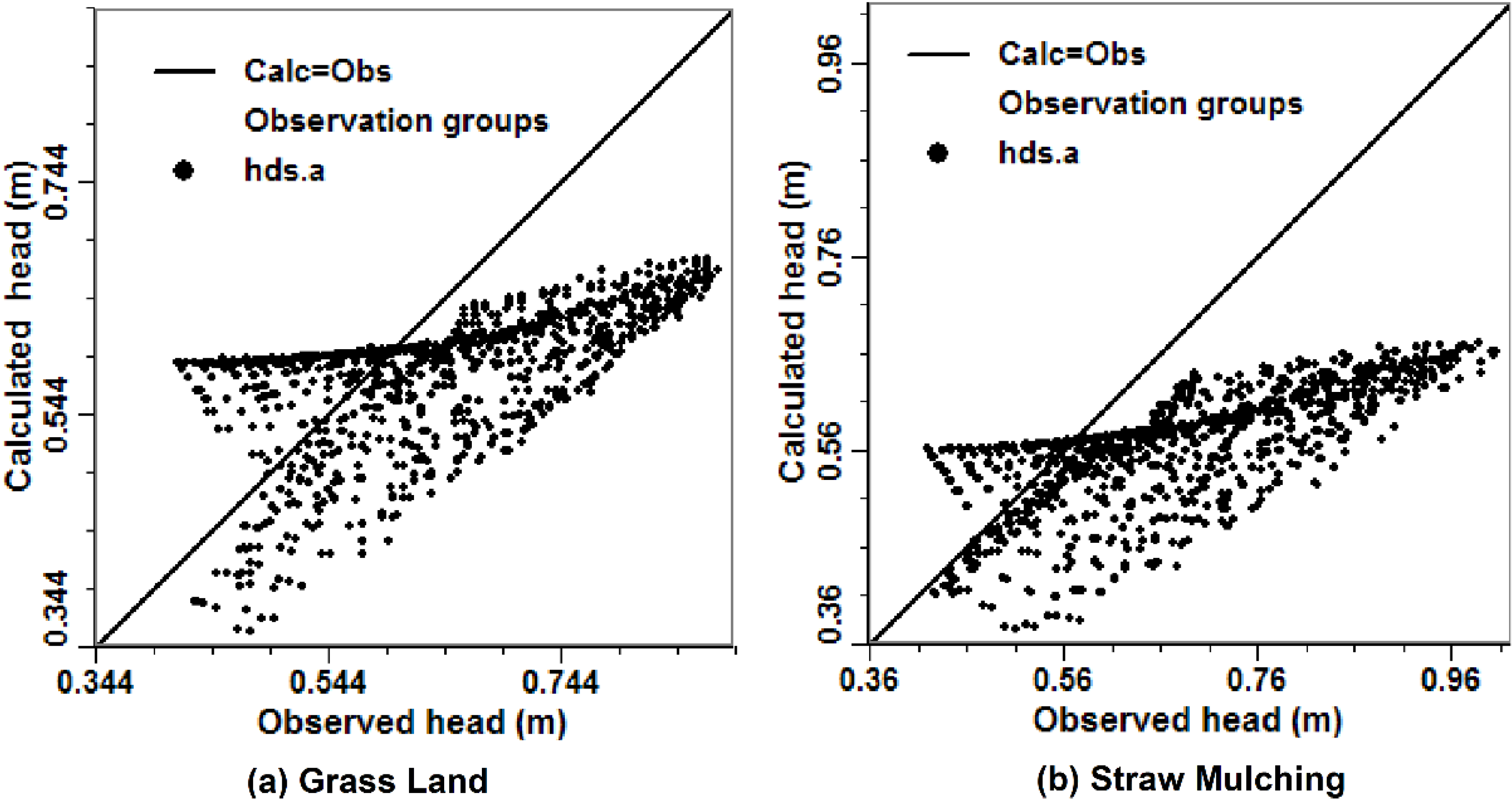
3.1. Model Calibration and the Key Parameters for Different Measures of Soil and Water Conservation

The hydraulic conductivity (Kx, Ky, and Kz), recharge rate (α), specific yield (Sy), and specific storage (Ss) were the main parameters of the MODFLOW model. Based on the simulated 75 mm/h rainfall experiment of the bare slope scenario, the main parameters of MODFLOW were calibrated and the model was verified under the simulated 45 mm/h rainfall experiment of the bare slope scenario [22].

The scatter graph of the calculated vs. observed values was the default calibration graph [25]. Overall the scatter graphs of calculated vs. observed values during the calibration period and the verification period (Figure 3a,b) showed that most of the points intersect the 45 degree line on the graph where X = Y. To be specific, in the space domain, the scatter graph of the 48 observation boreholes at any time point also matched well, such as the typical plot (Figure 3c,d); in the time domain, the time-series graph of the entire simulated period at any observation borehole also showed a good temporal trend, such as Figure 4.

Based on the statistical analysis of the model results, the residual mean (RM) for groundwater levels at the location observation boreholes was 0.02 cm and 0.04 cm during the calibration period and the verification period, respectively; the absolute residual mean (ARM) was 0.73 cm and 0.84 cm, respectively; the standard error of the estimate (SEE) was 0.12 cm for both, the normalized root mean squared (NRMS) was 4.15% and 4.26%, respectively; and the correlation coefficient (Cor) was 0.996 and 0.997, respectively.

From the scatter graphs and the calibration statistics between the observed and simulated hydraulic head, we can see that the simulated levels were consistent with the observed heads.

Then, to verify the availability of the model based on the simulated 75 mm/h rainfall experiments of the grassland and straw mulching scenarios, the models were simulated in different underlying surfaces. Figure 5 presents the scatter graph of calculated heads vs. observed levels. We can see that whether the simulations of the grassland scenario (Figure 5a) or the scatter graph for the straw mulching scenario (Figure 5b) showed the data points that deviated from the X = Y line, meaning that the calculated heads could not characterize the observed levels well. These results indicate that soil and water conservation measures have a great impact on the changes of groundwater regime.

Figure 3. Scatter graphs of the calculated heads vs. observed values for the whole period and t = 70 min during the calibration period (a, c) and the verification period (b, d). The groundwater heads are shown as dots and the solid lines mean the calculation heads are equal to the observed levels.

Figure 3. Scatter graphs of the calculated heads vs. observed values for the whole period and t = 70 min during the calibration period (a, c) and the verification period (b, d). The groundwater heads are shown as dots and the solid lines mean the calculation heads are equal to the observed levels.

Figure 4. Time-series graphs of the calculated vs. observed values during the calibration period (a) and the verification period (b). The observed heads are shown as larger dots and triangles. The calculated heads are shown as smaller dots and triangles with lines.

Figure 4. Time-series graphs of the calculated vs. observed values during the calibration period (a) and the verification period (b). The observed heads are shown as larger dots and triangles. The calculated heads are shown as smaller dots and triangles with lines.

Figure 5. The scatter graph of the calculated vs. observed values based on the calibrated parameters for different underlying surface: (a) Grass Land; (b) Straw Mulching. The groundwater heads are shown as dots and the solid lines mean the calculation heads are equal to the observed levels.

Figure 5. The scatter graph of the calculated vs. observed values based on the calibrated parameters for different underlying surface: (a) Grass Land; (b) Straw Mulching. The groundwater heads are shown as dots and the solid lines mean the calculation heads are equal to the observed levels.

Then, the most sensitive parameters for different underlying surfaces were calculated using the parameter inversion method based on the PEST-ASP program of Visual MODFLOW combined with manual parameter regulation. Through a many-times iterative solution, the results showed that the recharge rate (α), and specific yield of the three soil layers (Sy1, Sy2, and Sy3) were the most sensitive parameters under the grassland and straw mulching scenarios, and their more ideal values were calibrated (Table 1).

Table 1. The calibrated key parameters of the MODFLOW model.

The Key Parameters	α (10−5 m/s)	Sy1	Sy2	Sy3
Bare Slope	0.68	0.36	0.36	0.36
Grassland	1.72	0.22	0.22	0.27
Straw Mulching	1.92	0.072	0.072	0.26

Table 1. The calibrated key parameters of the MODFLOW model.

The Key Parameters	α (10−5 m/s)	Sy1	Sy2	Sy3
Bare Slope	0.68	0.36	0.36	0.36
Grassland	1.72	0.22	0.22	0.27
Straw Mulching	1.92	0.072	0.072	0.26

In this study, the recharge rate was mainly related to soil permeability and infiltration. Mulching the soil surface with a layer of plant residue could maintain and improve the soil stability and permeability and was also an effective method of increasing infiltration into the soil [7,10,11]. The specific yield was the water volume of an aquifer that was released from or taken into storage per unit of aquifer area per unit of change in the water table depth [28]. The specific yield was not only decided by the soil properties, the initial groundwater depth, and evaporation, but was also related to the decline rate, the drawdown time of the groundwater level, and the soil infiltration intensity [29,30]. The soil specific yield decreased with the increased rate of groundwater level decrease [31] and with increasing of soil infiltration intensity [32]. It was demonstrated that the soil and water conservation measures play an important role in weakening the surface runoff and strengthening the underground runoff [22].

Therefore, the verification results of the three scenarios (bare slope, grassland, and straw mulching) in water volume, hydraulic head, runoff and flow field of groundwater were considered to assess the application of Modflow in studying the impact of soil and water conservation measures on the groundwater regime.

3.2. Model Verification for Different Measures of Soil and Water Conservation

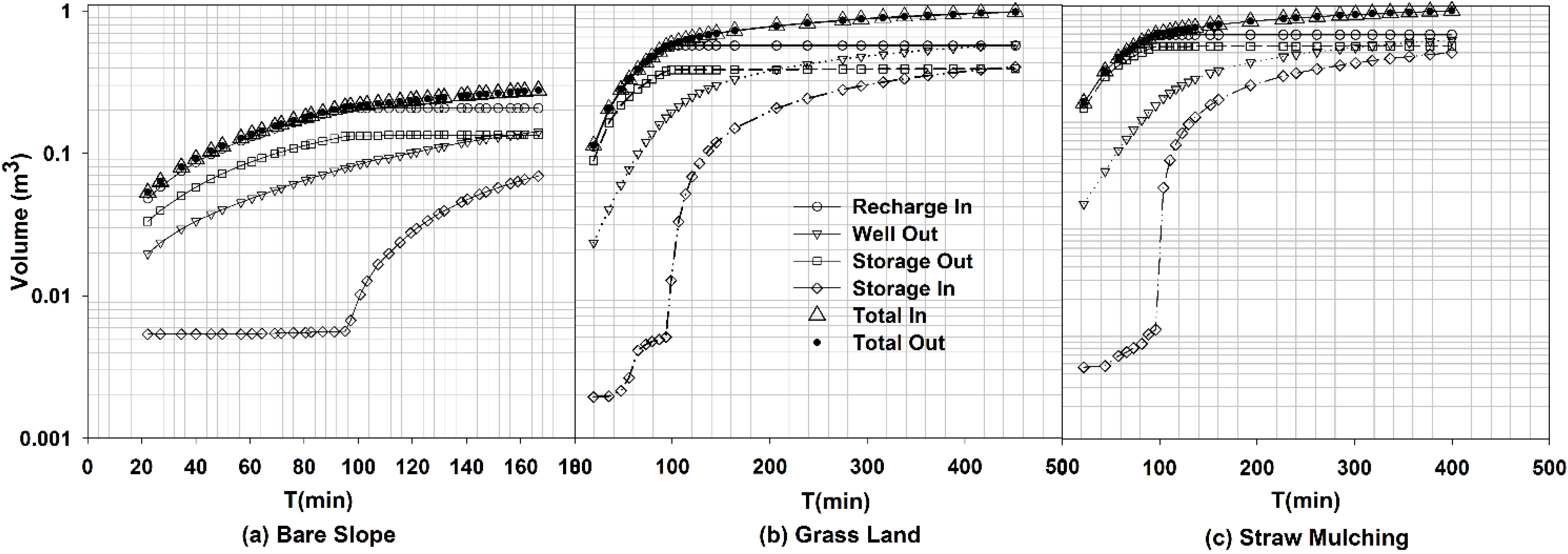
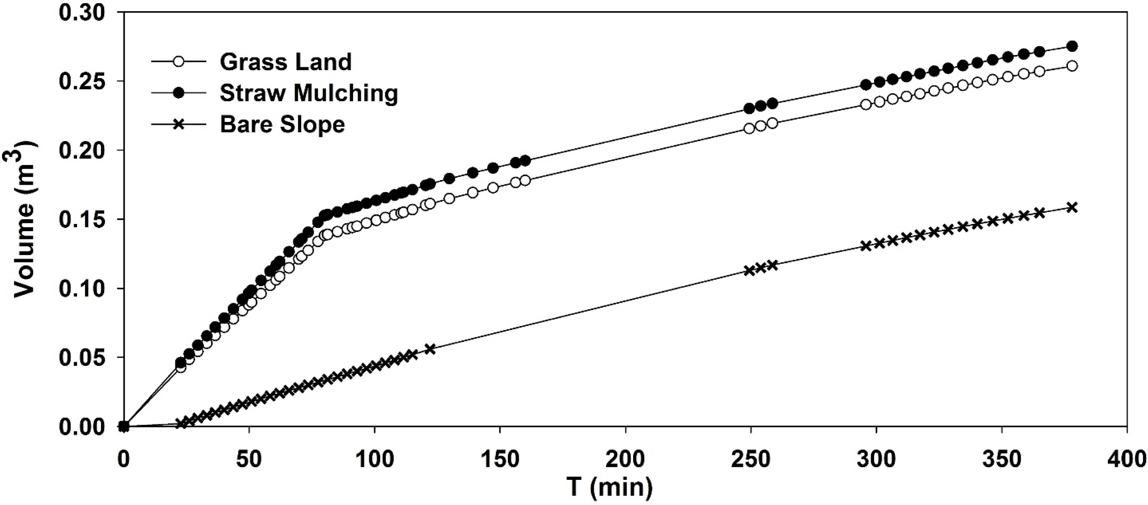
3.2.1. Verification of the Groundwater Balance

Figure 6 shows the flow mass balance graph of the bare slope, grassland and straw mulching scenarios. The flow mass balance graphs plot the temporal flows IN and OUT of the selected zone through the individual sources and sinks (flow boundary conditions and storage) [25]. At the end of the simulated period (t = 480 min) for the grassland scenario, the total volume flow into the entire system was 0.9111 m³ which increased the water storage by 0.3871 m³. The total volume flow out of the model was 0.9114 m³, which decreased the water storage by 0.3624 m³ and discharged 0.5490 m³ of recharge water. The mass balance error for the simulation inflow and outflow was 0.03%.

At the end of the simulated period (t = 454 min) for the straw mulching scenario, the total volume of flow into the entire system was 1.0182 m³, which increased the water storage by 0.4331 m³. The total volume flow out of the model was 1.0196 m³, which decreased the water storage by 0.4596 m³ and discharged 0.5600 m³ of the recharge water. The mass balance error for the simulation inflow and outflow was 0.13%. For the bare slope scenario, the mass balance error was 0.22% [26]. The results of the simulation may generally be considered acceptable, provided that the models were also calibrated [25].

Figure 6. The flow mass balance graphs of the bare slope (a); grassland (b) and straw mulching scenarios (c).

Figure 6. The flow mass balance graphs of the bare slope (a); grassland (b) and straw mulching scenarios (c).

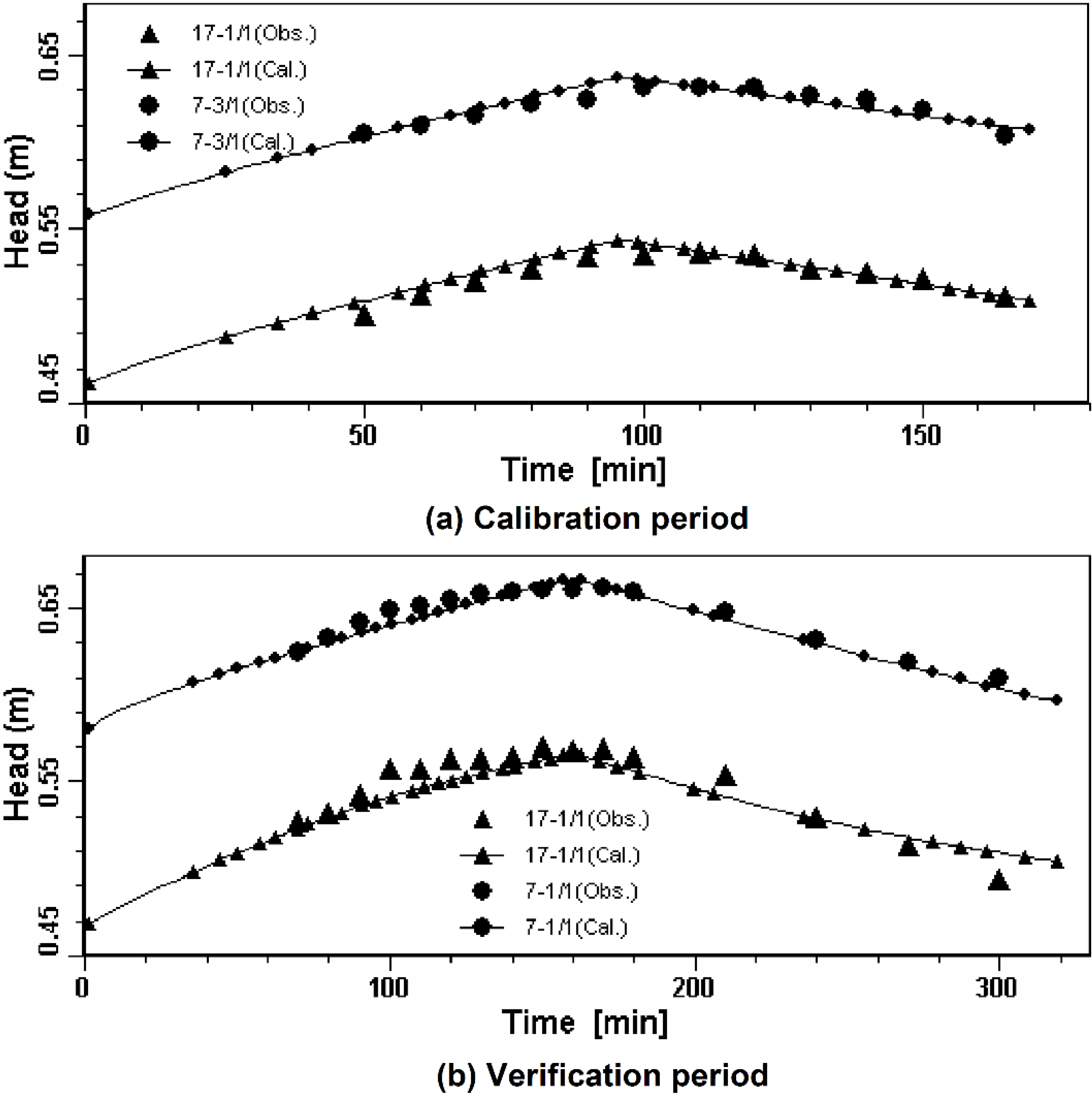
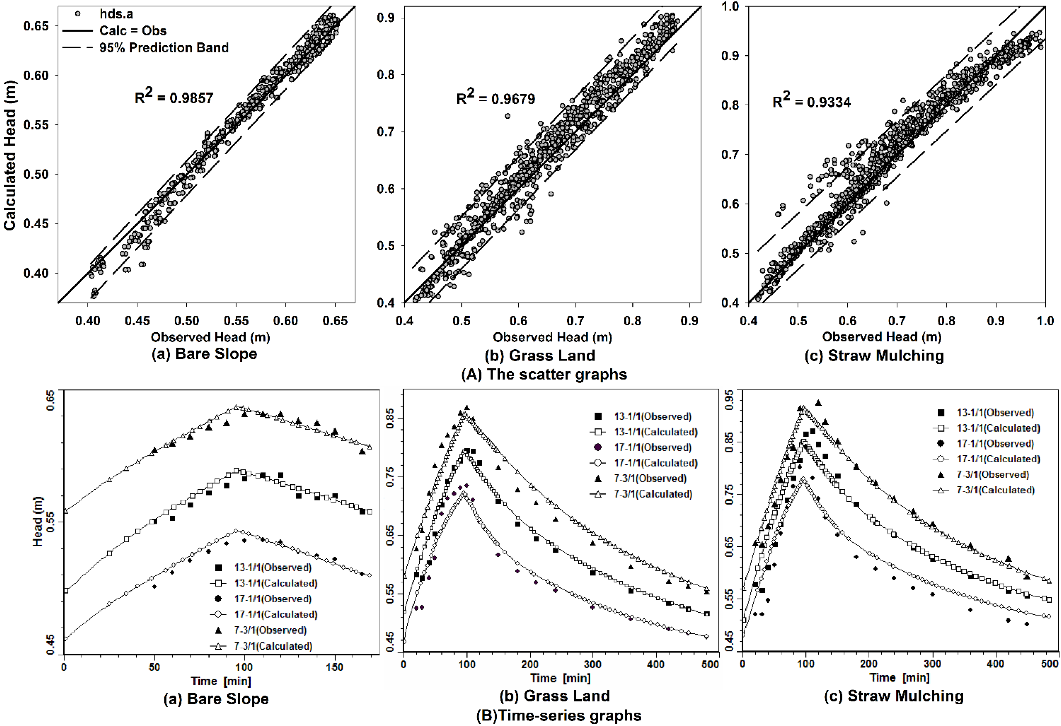
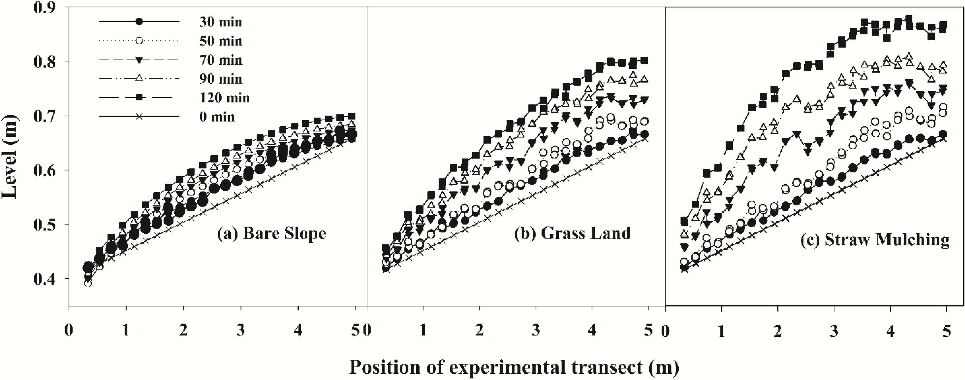
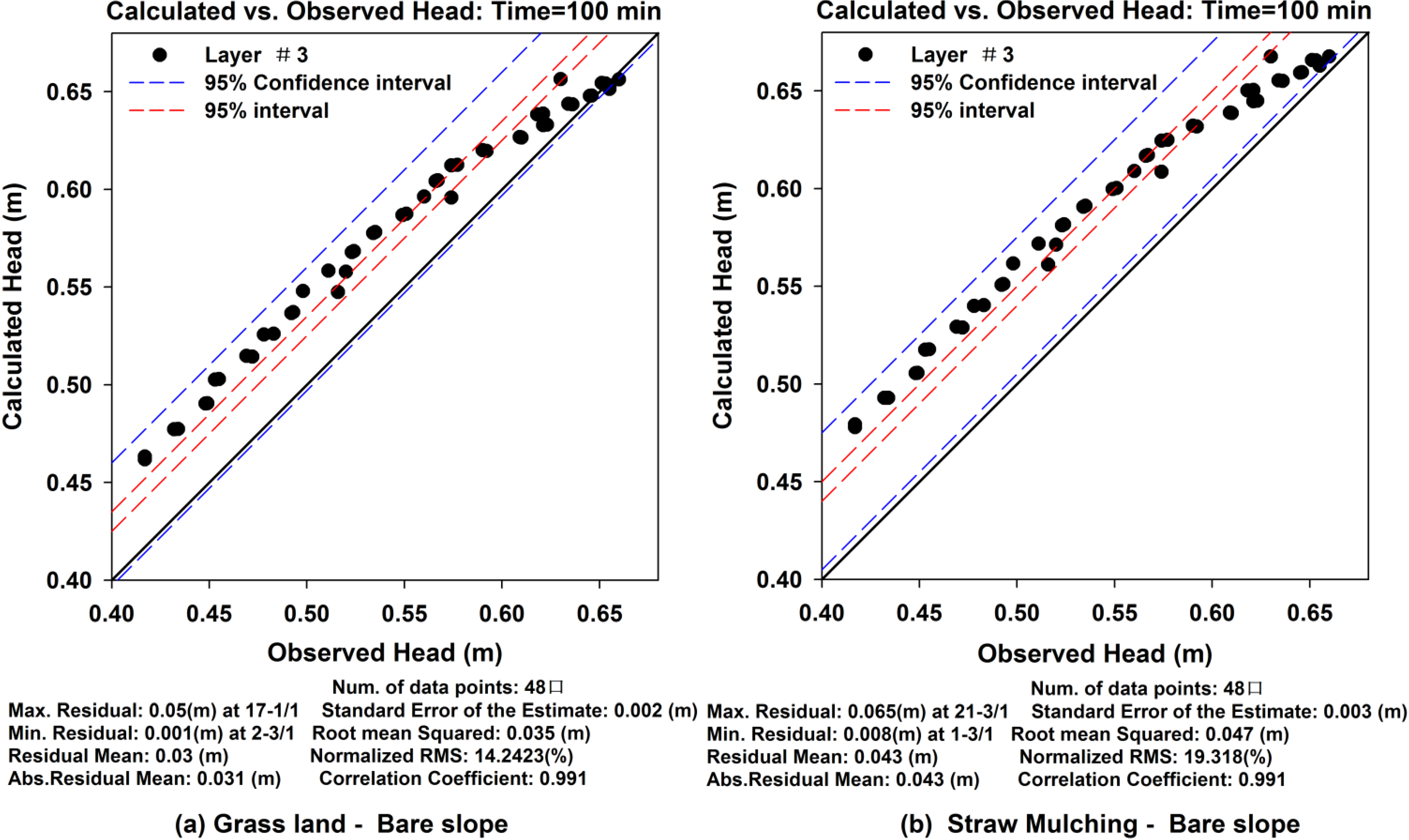
3.2.2. Verification of the Groundwater Level

The scatter graphs of bare slope, grassland and straw mulching scenarios (Figure 7A) showed that most of the data points intersect the 45 degree line on the graph where X = Y. These results represented an ideal calibration in which the simulated hydraulic heads were consistent with the observed heads. Transient simulations contain many different observation times for each observation point; therefore, the quality of the model calibration will likely change throughout the simulation, making it important to evaluate the calibration at different times throughout the simulation [25]. Figure 7B shows the time-series graph of the entire simulated period of three observation boreholes for three scenarios, which also showed the same temporal trend between the observed levels and the calculated heads.

The calibration statistics are reported in the footer of the calibration plot window when the calculated vs. observed scatter graph is displayed [25] and they could be exported for every observation time, which was good for controlling the quality of the model calibration throughout the simulation. Therefore, the mean values of calibration statistics throughout the simulation period could be analyzed (Table 2), providing a more accurate comparison between the calculated values and the observed data.

Based on the comparison results of the scatter graphs, time-series graphs and calibration statistics between the observed heads and simulated levels for bare slope, grassland and straw mulching scenarios, we could see the model was able to reasonably reproduce the groundwater level conditions.

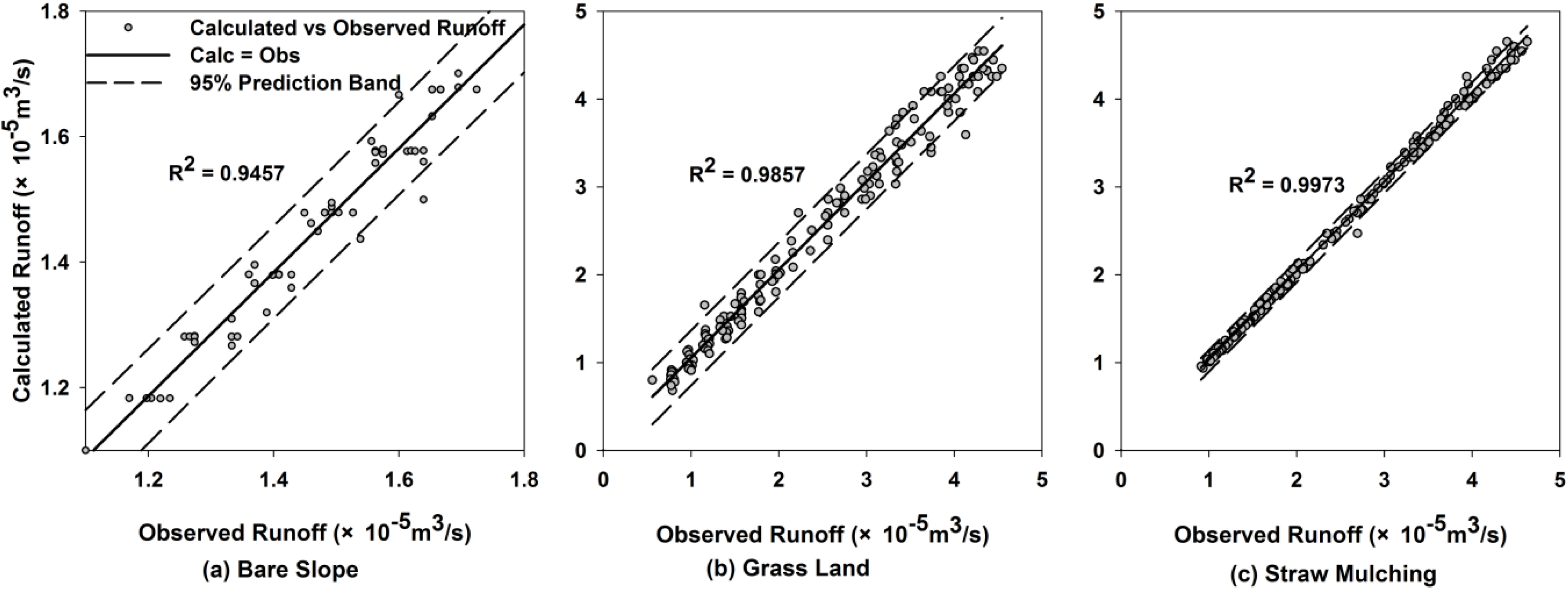
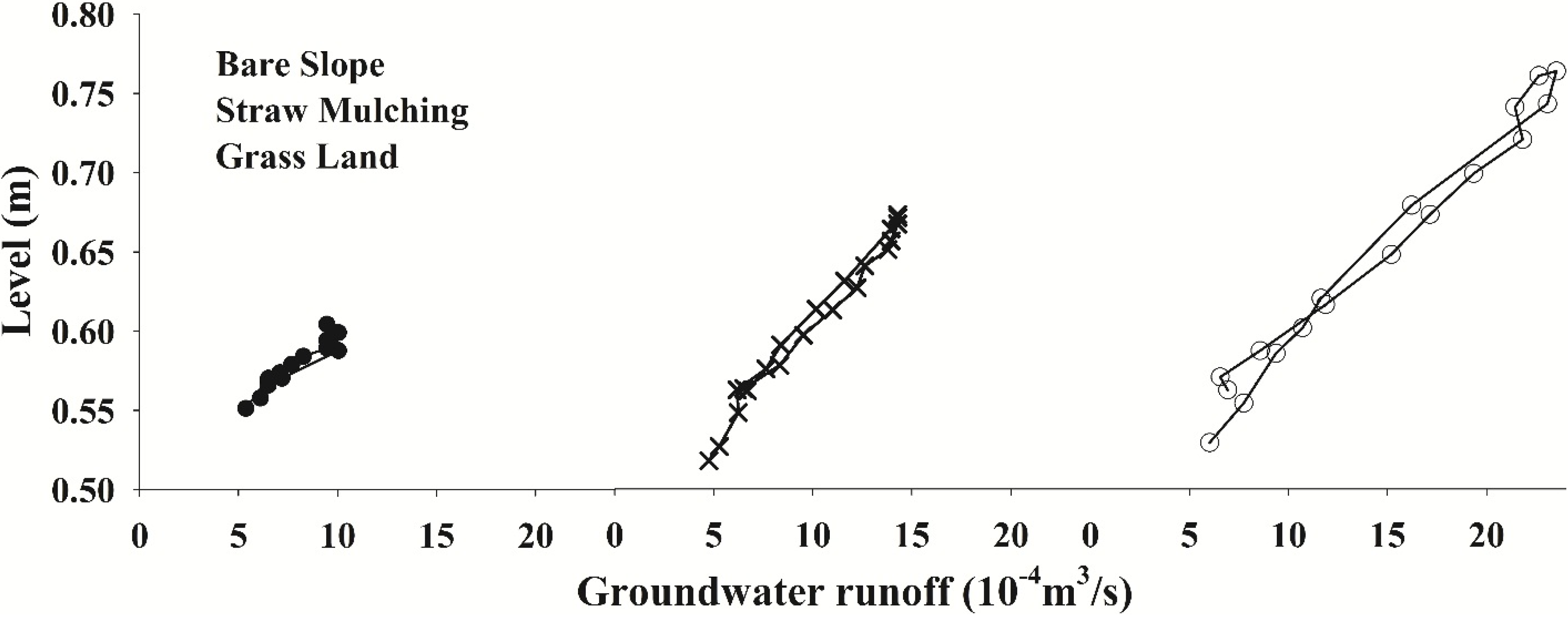
3.2.3. Verification of the Groundwater Runoff

Figure 8 shows the scatter graphs between the observed groundwater runoff and the simulated flow of the bare slope, grassland and straw mulching scenarios. Most of the data points intersected the 45 degree line on the graph where X = Y, indicating that the simulated groundwater flows were consistent with the observed values. From Figure 8, we can see that the results of the bare slope scenario were the worst compared the three scenarios; its simulation accuracy was slightly worse, and the 95% prediction interval was slightly larger. However, the correlation coefficients of the three scenarios were all greater than 0.94. Therefore, the model could be used for groundwater flow simulation in this study.

Figure 7. The graphs of the calculated vs. observed heads for three scenarios: (a) Bare Slope; (b) Grass Land; (c) Straw Mulching; (A) The scatter graphs; (B) Time-series graphs.

Figure 7. The graphs of the calculated vs. observed heads for three scenarios: (a) Bare Slope; (b) Grass Land; (c) Straw Mulching; (A) The scatter graphs; (B) Time-series graphs.

Table 2. The error indexes of the calculated vs. observed values.

The Evaluation Indexes	RM/m	ARM/m	SEE/m	RMS/m	NRMS/%	Cor
Bare Slope	0.0002	0.007	0.001	0.010	4.146	0.996
Grassland	0.012	0.021	0.003	0.025	8.336	0.981
Straw Mulching	0.018	0.028	0.004	0.035	9.932	0.983

Table 2. The error indexes of the calculated vs. observed values.

The Evaluation Indexes	RM/m	ARM/m	SEE/m	RMS/m	NRMS/%	Cor
Bare Slope	0.0002	0.007	0.001	0.010	4.146	0.996
Grassland	0.012	0.021	0.003	0.025	8.336	0.981
Straw Mulching	0.018	0.028	0.004	0.035	9.932	0.983

Figure 8. The scatter graph of the calculated vs. observed groundwater runoff for three scenario: (a) Bare Slope; (b) Grass Land; (c) Straw Mulching.

Figure 8. The scatter graph of the calculated vs. observed groundwater runoff for three scenario: (a) Bare Slope; (b) Grass Land; (c) Straw Mulching.

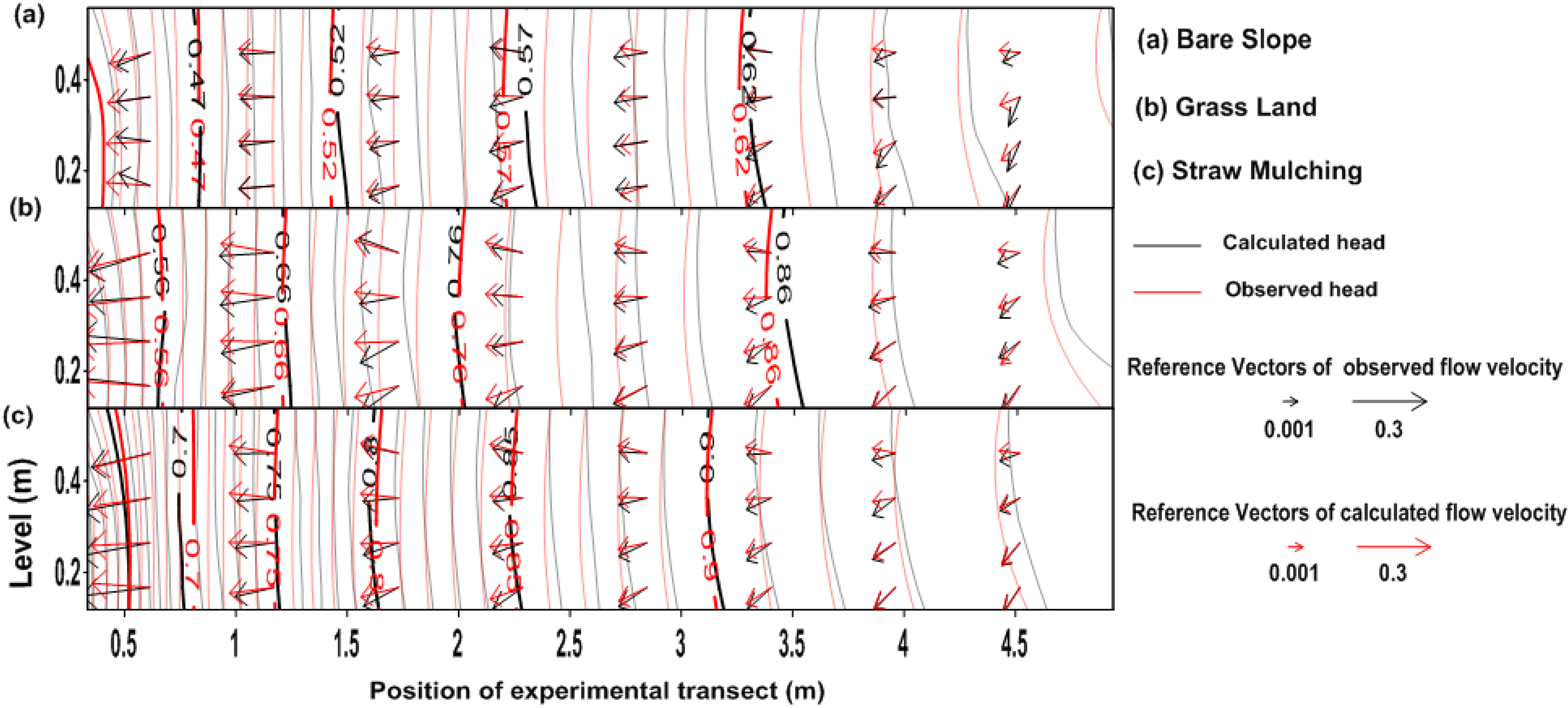
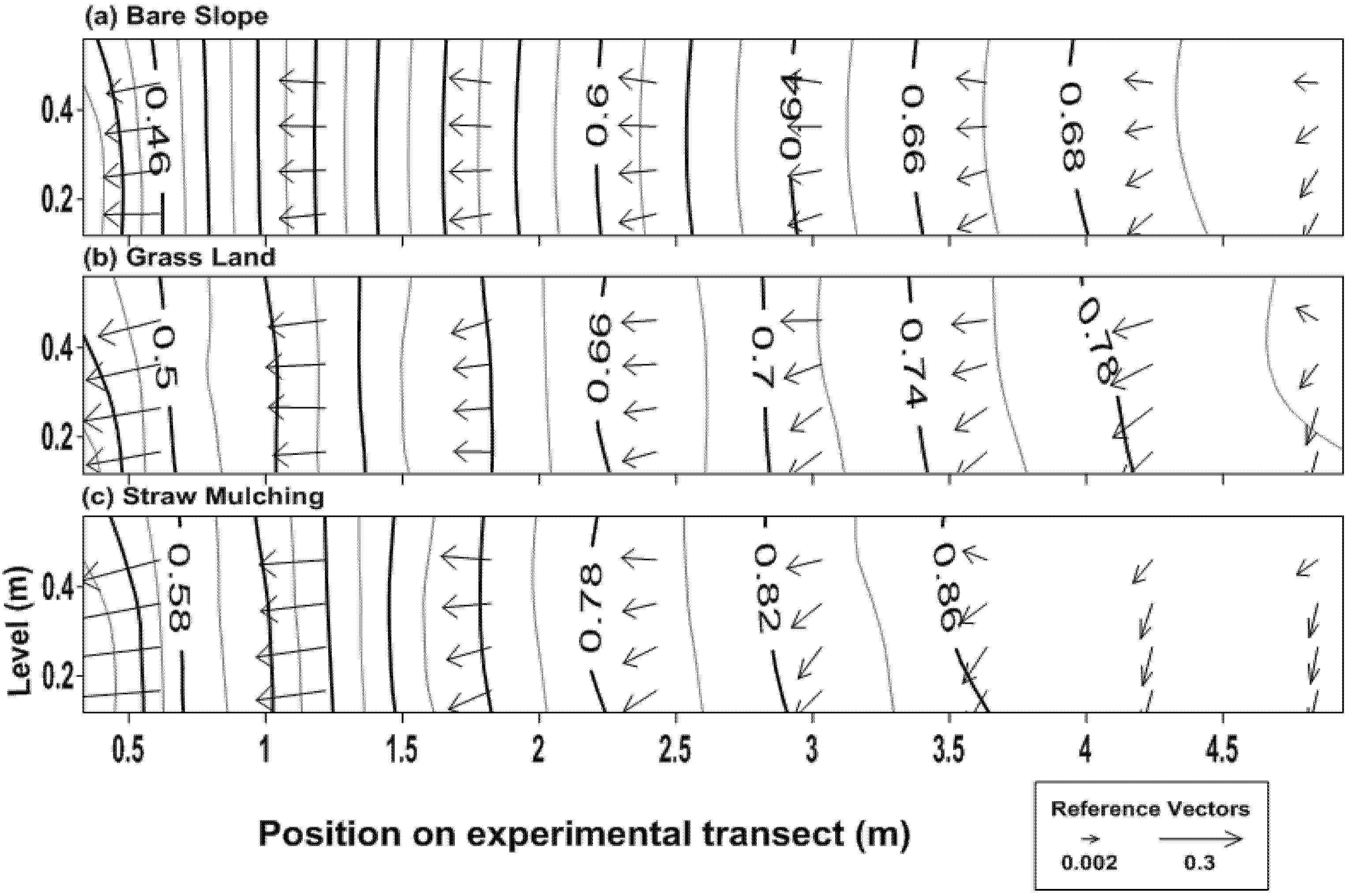
3.2.4. Verification of the Groundwater Flow Field

The changes in the groundwater recharge, level and flow were the results of variation in the groundwater flow field; therefore, it is necessary to verify the velocity and direction of groundwater flow under different soil and water conservation measures. The flow fields of groundwater at 100 min for different scenarios (Figure 9) showed that the calculated groundwater flow field could reflect the tendency and law of simulated groundwater flow.

Figure 9. Flow field of the groundwater at 100 min for three scenarios: (a) Bare Slope; (b) Grass Land; (c) Straw Mulching (The direction of reference vectors stands for flow direction of groundwater and the size of reference vectors only means high or low velocity of flow, not the exact value of flow rate).

Figure 9. Flow field of the groundwater at 100 min for three scenarios: (a) Bare Slope; (b) Grass Land; (c) Straw Mulching (The direction of reference vectors stands for flow direction of groundwater and the size of reference vectors only means high or low velocity of flow, not the exact value of flow rate).

The fitting situation could be roughly divided into two categories. One situation was located at the outflow region of the model, where hydraulic gradient was smaller. The calculated flow field was better fitted for the observed flow field. The model could reflect the dynamic tendency and law of groundwater flow well at the outflow region. The other situation was located at the inflow region of the model, where the hydraulic gradient was larger. The fitting situation was not as good as that in the outflow region due to the intense amplitude of the groundwater level. There was a small gap between the calculated levels and the observed heads, but the tendency and law of the flow field were always the same. Overall, not only the simulation morphology but also the flow directions of the groundwater flow field were consistent with the measured flow field.

The results demonstrate that this model could be used for different underlying surfaces. However, different calibrated parameters were required for different soil surfaces, and the recharge rate (α) and specific yield of the three soil layers (Sy1, Sy2, and Sy3) were the most sensitive parameters. Therefore, α, Sy1, Sy2, and Sy3 should be calibrated at least according to the actual situation when the underlying surface changes in the studying area, and the impacts of soil and water conservation measures construction measures on the groundwater were studied based on the calibrated bare slope model and compared to the corresponding results of lawn and straw mulching from simulated experiments. Additionally, the impacts of soil and water conservation measures destruction on groundwater were studied based on the calibrated grassland and straw mulching models and compared to the corresponding results of the bare slope scenario from simulated experiments.

3.3. The Impact of Soil and Water Conservation Measures Construction on Groundwater

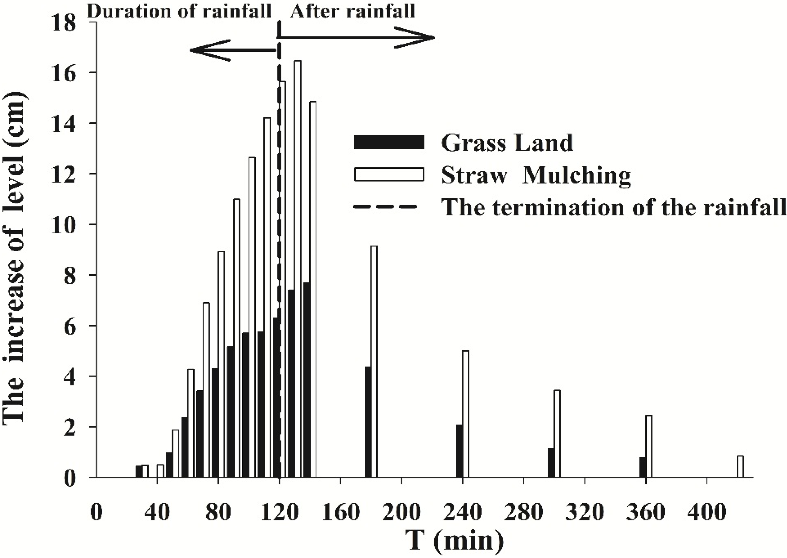
3.3.1. Response of Groundwater Recharge and Runoff

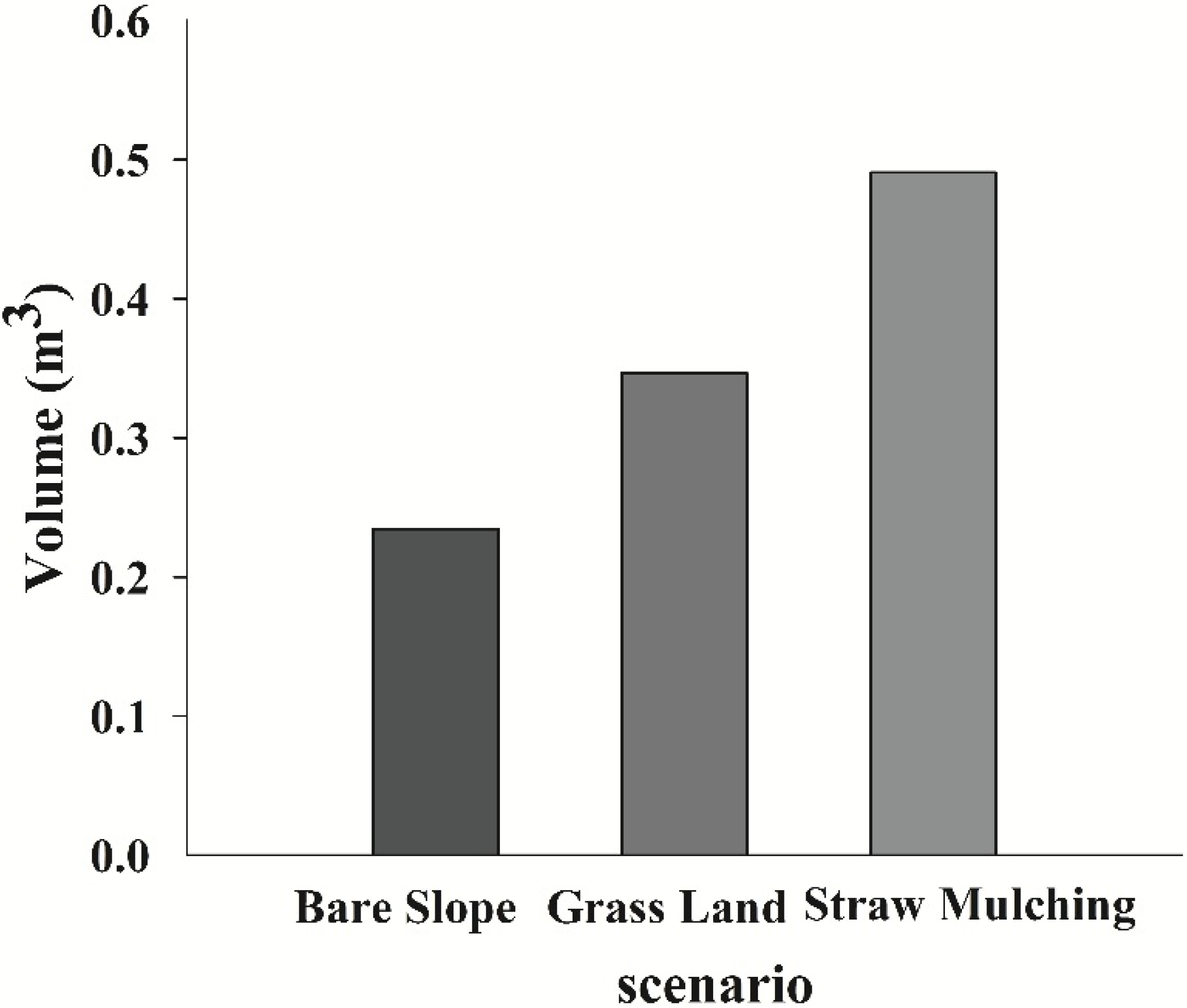
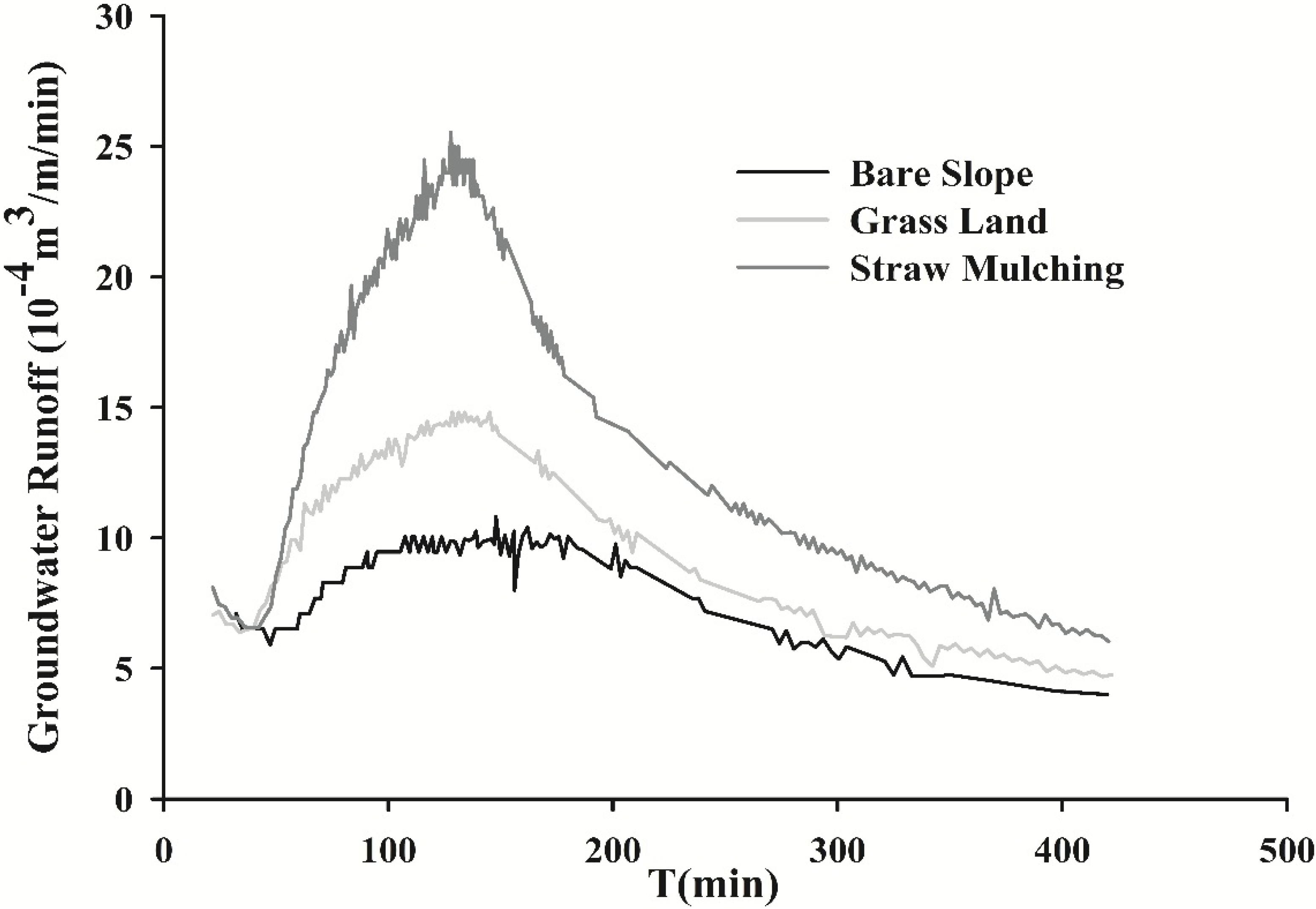
Then, based on the calibrated groundwater transient flow model, the rainfall intensity of 60 mm/h of bare slope scenario was predicted for comparison with the corresponding groundwater recharge, runoff, level and stage-discharge of the lawn and straw mulching experiments. Mass balance which is one of the key indicators of a successful simulation [25] was analyzed first. The time series plotted the temporal flows IN and OUT of the system, and the mass balance error for the simulation inflow and outflow of the model was 1.47% < 2%.

Figure 10 presents the accumulated recharge of groundwater for different scenarios during the simulated period (0–420 min) and shows that measures of soil and water conservation might lead to a greater proportion of rainfall being infiltrated and available for groundwater recharge. It is apparent that mulching the soil surface with a layer of plant residue is an effective method of conserving water because it reduced surface runoff, increased the infiltration of water into the soil and retarded soil erosion [7]. The cumulative volume of groundwater increased 1.5 times and 2 times for the grassland and straw mulching scenarios, respectively, compared to that of the bare slope scenario.

Figure 10. Comparison of accumulated volume of the groundwater among three scenarios.

Figure 10. Comparison of accumulated volume of the groundwater among three scenarios.

Groundwater runoff had the same trend with accumulated recharge in the sequence of size for the three different scenarios. The groundwater runoff of the straw mulching scenario was the highest, the grassland scenario showed intermediate runoff, and that of the bare slope scenario was the lowest. The maximum difference in a per unit width flux varied from 10.81 × 10⁻⁴ m³/m/min for the bare slope scenario to 25.53 × 10⁻⁴ m³/m/min for the straw mulching scenario, whereas the corresponding values of the model average difference were 8.29 × 10⁻⁴ m³/m/min and 15.51 × 10⁻⁴ m³/m/min, respectively. Similarly, compared to that of the bare slope scenario, the maximum and average increase in the grassland scenario were smaller than those in the straw mulching scenario. In the time domain, there were significant differences in the magnitude of discharge among the three scenarios with a constant amount of rainfall (120 mm), but all of the time-series lines of groundwater runoff (Figure 11) exhibited similar trends in which the groundwater runoff initially increased sharply with the rainfall but then decreased gradually after its termination. The increased average groundwater runoff during the simulated period for the straw mulching scenario was more than twice as large as that for the grassland scenario compared to that of the bare slope scenario. Table 3 summarizes the changes in the average and maximum values and percent change in the groundwater flow among the three scenarios. The groundwater recharge very strongly depended on the land-use type [33].

Figure 11. Time-series graphs of the groundwater runoff among three scenarios.

Figure 11. Time-series graphs of the groundwater runoff among three scenarios.

Table 3. Difference value and change of the groundwater runoff and volume in three scenarios.

Scenario		Runoff
		Value (10−4 m3/m/min)	Change (%)
Average	Bare Slope	8.29	0
	Grassland	10.19	22.9
	Straw Mulching	15.51	87.1
Maximum	Bare Slope	10.81	0
	Grassland	14.82	37.1
	Straw Mulching	25.53	136.2

Table 3. Difference value and change of the groundwater runoff and volume in three scenarios.

Scenario		Runoff
		Value (10−4 m3/m/min)	Change (%)
Average	Bare Slope	8.29	0
	Grassland	10.19	22.9
	Straw Mulching	15.51	87.1
Maximum	Bare Slope	10.81	0
	Grassland	14.82	37.1
	Straw Mulching	25.53	136.2

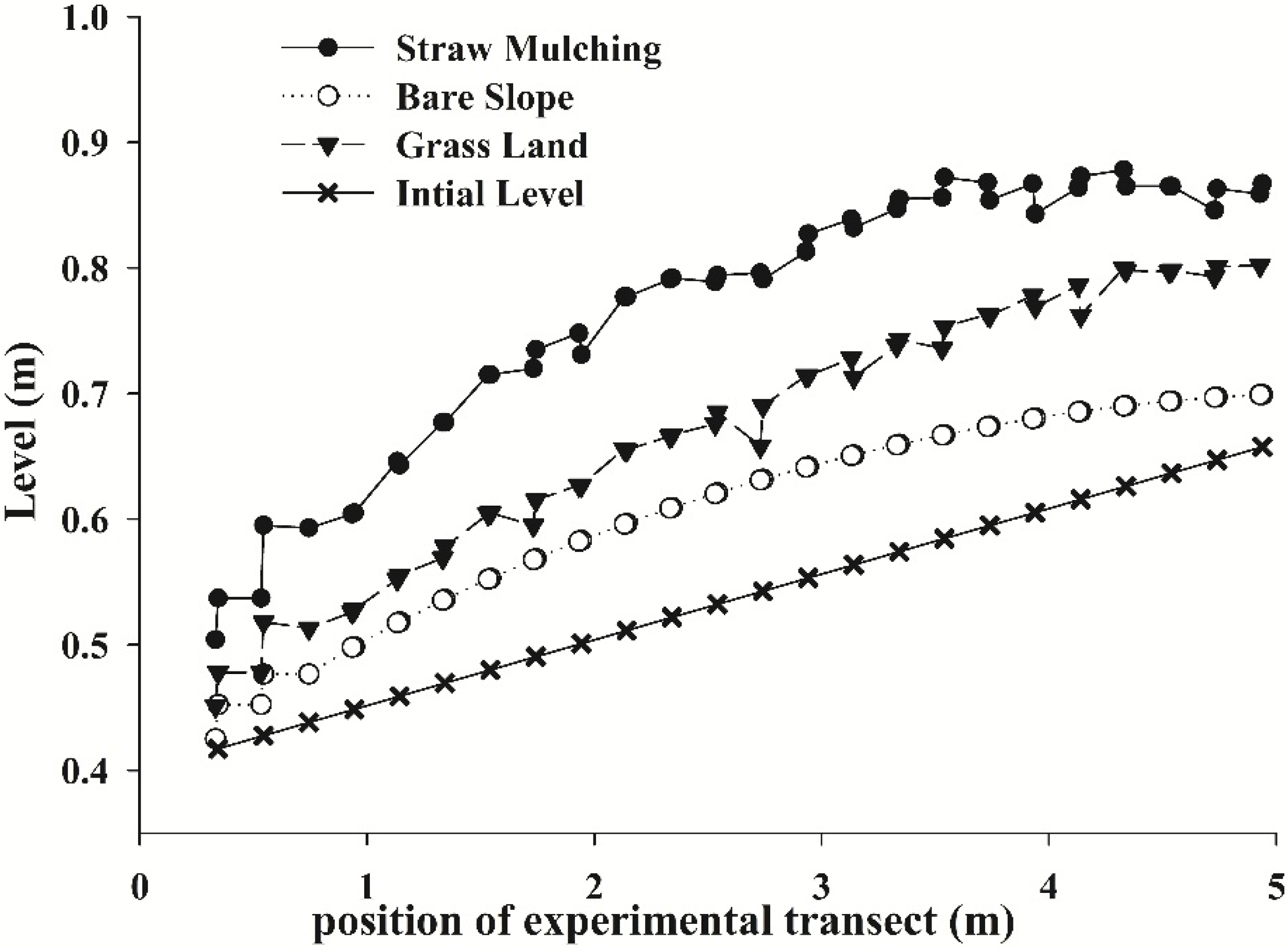
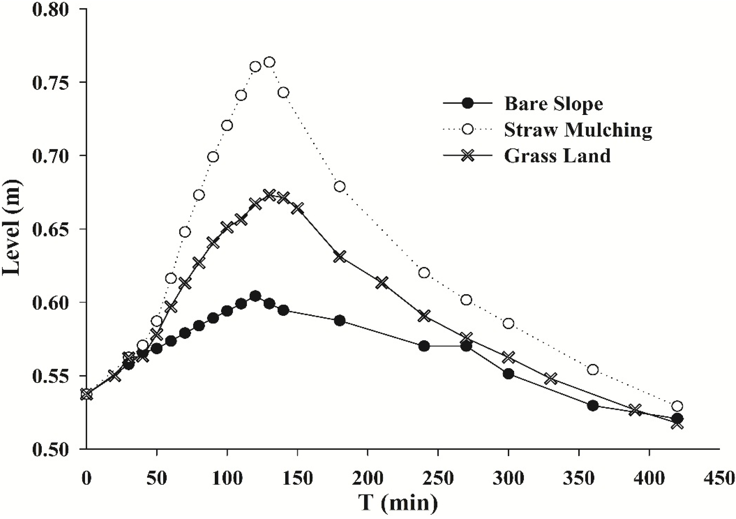
3.3.2. Response of the Groundwater Level

The groundwater level might be changed due to a variation in the groundwater runoff. The analyzed differences in the magnitude of groundwater level fluctuations arose from land cover variations (Figure 12, Figure 13, Figure 14, Figure 15, Figure 16 and Figure 17). During the rainfall (t = 0–120 min), although there were significant differences in the magnitude changes in the groundwater level among the different scenarios, all of the time-series graphs for the three scenarios exhibited similar increasing trends (Figure 12). The average level across the entire profile of the straw mulching scenario increased by a factor of approximately 13.2%, to an average change value of 7.65 cm compared to the bare slope scenario and the average level of the grassland event increased somewhat less, approximately 7.43%, during the rainfall. In the space domain, the levels increased for every site. After the termination of the rainfall (t = 120 min) (Figure 13 and Figure 14), the average level increased from 7.88 cm to 20.48 cm with a mean value of 15.64 cm, increased by 25.88% across the entire profile for the straw mulching scenario and increased by 10.41% for the grassland scenario compared to the bare slope scenario.

Figure 12. Comparison of the magnitude of the groundwater level fluctuations arisen from land cover variations (t = 0–120 min).

Figure 12. Comparison of the magnitude of the groundwater level fluctuations arisen from land cover variations (t = 0–120 min).

Figure 13. Comparison of the magnitude of the groundwater level fluctuations after termination of the rainfall (t = 120 min).

Figure 13. Comparison of the magnitude of the groundwater level fluctuations after termination of the rainfall (t = 120 min).

Figure 14. Flow field of the groundwater after termination of the rainfall for three scenarios: (a) Bare Slope; (b) Grass Land; (c) Straw Mulching.

Figure 14. Flow field of the groundwater after termination of the rainfall for three scenarios: (a) Bare Slope; (b) Grass Land; (c) Straw Mulching.

A comprehensive analysis of the average groundwater levels at 48 observed wells during the simulated period (0–420 min) showed noticeable increasing trends for straw mulching/grassland scenarios compared to those of the bare slope scenario (Figure 15). Figure 15 shows a scatter plot of the calculated levels vs. the observed heads, showing that the data points were under the X = Y line; therefore, the calculated values of the bare slope scenario were less than the observed values of the straw mulching/grassland scenarios. Larger changes in the mean groundwater level occurred in the straw mulching scenario, which showed an increase of 7.32 cm. The time-series average groundwater levels across the entire profile for different scenarios are presented in Figure 16, which shows that the groundwater runoff initially increased sharply but then decreased gradually after the termination of the rainfall when water was not continually provided. The greatest mean groundwater level for the bare slope scenario was 60.4 cm and occurred at t = 120 min, whereas those for straw mulching and grassland scenarios were 76.4 cm and 67.3 cm, respectively, and occurred at t = 130 min (Figure 17). The measures of soil and water conservation significantly postponed runoff generation and promoted the groundwater head. The increases in the average groundwater runoff for the straw mulching and grassland scenarios were more than twice as large as those for the grassland scenario compared to the bare slope scenario. The largest mean increase in the groundwater level for the straw mulching scenario was 27.5% and occurred at t = 130 min, whereas that for the grassland scenario increased by 12.9% and occurred at t = 140 min. Compared to the bare slope scenario, the increases in the mean groundwater levels varied from 3.91 cm for the grassland scenario to 7.32 cm for the straw mulching scenario during the simulated period.

Figure 15. Time-series graphs of the groundwater level fluctuations among three scenarios during the simulated period.

Figure 15. Time-series graphs of the groundwater level fluctuations among three scenarios during the simulated period.

Figure 16. Time-series graphs of the groundwater level fluctuations among three scenarios during the simulated period.

Figure 16. Time-series graphs of the groundwater level fluctuations among three scenarios during the simulated period.

Figure 17. Time-series graphs of the groundwater level increase with underlying surface changing.

Figure 17. Time-series graphs of the groundwater level increase with underlying surface changing.

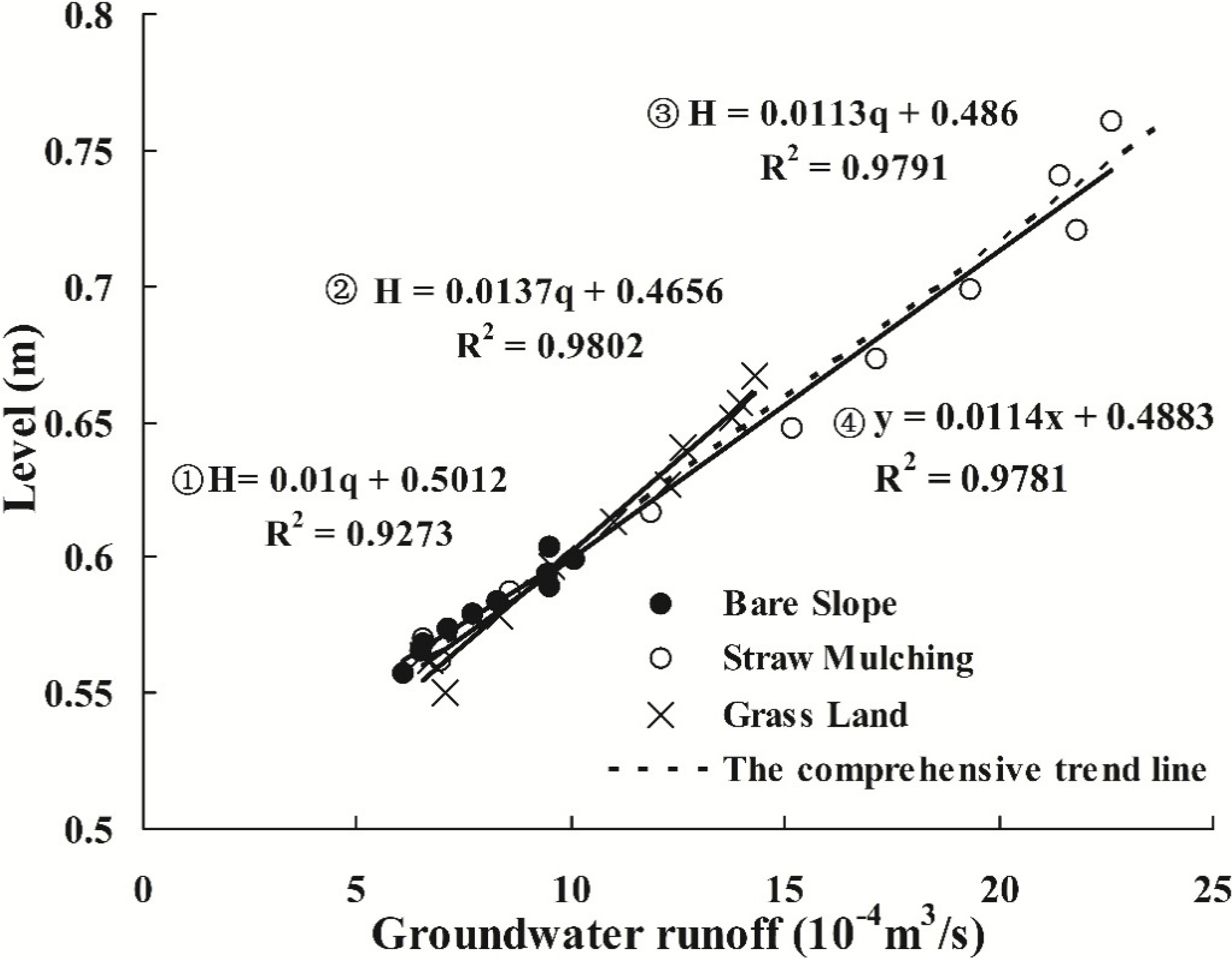
3.3.3. Response of the Stage-Discharge Relationship of the Groundwater

Setting up a stage-discharge relationship is an important part of the processing of stream flow data [34]. It has become a common practice to convert records of water stages (which are easier and less expensive to measure) into discharges by using a pre-established stage-discharge relationship [35], especially for groundwater. Figure 18 shows the stage-discharge relationship of groundwater for three scenarios during rainfall. The level is the time-series average level across the entire profile and the corresponding discharge out of the well. From Figure 18, we can see that when the land-use converted from bare slope to grassland and straw mulching, the magnitude of the corresponding rating curve increased, whereas the three rating curves had the same trend. The average level increased linearly with the increased of discharge. For the bare slope scenario, the discharge of the groundwater increased from 6.1 × 10⁻⁴ m³/m to 9.5 × 10⁻⁴ m³/m, and the mean level increased from 55.8 to 59.4 cm with a mean value of 57.7 cm. Comparatively, for the grassland and straw mulching scenarios, the discharge increased approximately 3.2 and 2.1 times, respectively, during the rainfall.

The dynamic relationship between the stage and the discharge could be determined via mathematical relationships [36]. Equations ①, ② and ③ in Figure 18 show the relationship between the stage and discharge for the bare slope, grassland and straw mulching scenarios, respectively. Meanwhile, most of the data points intersect the comprehensive trend line on the graph. Therefore, a regression analysis was conducted to yield a comprehensive relationship among the three scenarios, as in Equation ④ in Figure 18. The graph showed an almost perfect match except for a slight deviation and a correlation coefficient of R = 0.989. Thus, the comprehensive relationship could be very effectively used to map the rating curves.

Figure 18. Stage-discharge relationship of the groundwater for three scenarios during rainfall (t = 0–120 min).

Figure 18. Stage-discharge relationship of the groundwater for three scenarios during rainfall (t = 0–120 min).

A comprehensive analysis of the stage-discharge relationship during the simulated period (0–420 min) (Figure 19) showed that the observed measurements of stage and discharge did not form a unique relationship and that a single value of the stage did not correspond to a single value of discharge. The relationship between the stage and discharge were loop-rating curves. With the underlying surface being converted from bare slope to grassland and straw mulching, the stage-discharge relationship was the same, but the range of the rating curve expanded gradually.

Figure 19. Stage–discharge relationship of the groundwater for three scenarios during rainfall (t = 0–120 min).

Figure 19. Stage–discharge relationship of the groundwater for three scenarios during rainfall (t = 0–120 min).

3.4. The Impact of Soil and Water Conservation Measures Destruction on Groundwater

To assess the effects of grassland and straw mulching changes to bare slope on the groundwater recharge and hydraulic head, grassland and straw mulching scenarios of a 90-mm/h rainfall intensity were simulated based on the calibrated and verified MODFLOW model. Then, the simulated results were compared with the observed results of the bare slope scenario under the same 90 mm/h rainfall intensity conditions.

Figure 20 compares the changes in the accumulated recharge volume with scenarios of conversion from grassland and straw mulching to bare slope. As a result, the cumulative curve of straw mulching was the highest, the grassland showed intermediate values, and that of the bare slope was the lowest. Hence, there was a significant decrease when the straw mulching and grassland measures were destroyed. At the end of simulation period, the calculated groundwater volumes were 0.275 m³ and 0.261 m³ in the straw mulching and grassland scenarios, respectively, whereas the volume was only 0.159 m³ in the observed bare slope scenario. Therefore, when the land-use converted from straw mulching and grassland to bare slope, the volume of the groundwater recharge decreased by 42.2% and 39.1%, respectively.

Figure 20. The time-series graphs of the accumulated groundwater volume under three scenarios.

Figure 20. The time-series graphs of the accumulated groundwater volume under three scenarios.

The influence of the scenarios of conversion from grassland and straw mulching to bare slope on groundwater levels at t = 100 min is shown in Figure 21. Figure 21a shows scatter plots of the calculated levels of the grassland scenario vs. the observed heads of the bare slope scenario and Figure 21b shows a graph of the calculated levels of the straw mulching scenario vs. the observed values of the bare slope scenario. As Figure 21 shows, the data points were above the X = Y line; therefore, the calculated values were larger than the observed values. Because the calculated values of Figure 21a,b were based on the groundwater levels of grassland and straw mulching scenarios, respectively, the observed values represented the groundwater levels of the bare slope scenario. Therefore, the groundwater levels of the bare slope were greater than the levels of grassland and straw mulching, indicating that the groundwater levels decreased with the land-use conversion from grassland to bare slope and even more with the land-use conversion from straw mulching to bare slope.

Figure 21. The scatter graph of the calculated vs. observed values when the underlying surface converted from straw mulching and grassland to bare slope. (a) shows the compared results when the underlying surface converted from straw mulching to bare slope; (b) shows the compared results when the underlying surface converted from grassland to bare slope. The groundwater heads are shown as dots and the solid lines mean the calculation heads are equal to the observed levels.

Figure 21. The scatter graph of the calculated vs. observed values when the underlying surface converted from straw mulching and grassland to bare slope. (a) shows the compared results when the underlying surface converted from straw mulching to bare slope; (b) shows the compared results when the underlying surface converted from grassland to bare slope. The groundwater heads are shown as dots and the solid lines mean the calculation heads are equal to the observed levels.

4. Conclusions

Based on rainfall experiments, MODFLOW was calibrated and verified for bare slope, grassland and straw mulching scenarios. The measures had an effective impact on the parameters of MODFLOW. The model that was calibrated and validated under bare slope scenario could not be applied for grassland and straw mulching scenarios under the same conditions. The recharge rate (α) and specific yield of the three soil layers (Sy1, Sy2, and Sy3) of model were the most sensitive parameters to the changes in the underlying surface.

MODFLOW could be used to study the impact of soil and water conservation measures on the groundwater regime. The verification results of the bare slope, grassland and straw mulching scenarios showed that: (1) the mass balance errors of the inflow and outflow system for three scenarios were all less than 2%; (2) both the values and the tendency of the simulated groundwater level were consistent with calculated heads and the errors in the evaluation indexes were within the permitted range; (3) the simulated groundwater flow was consistent with the observed values and the correlation coefficients were greater than 0.97; and (4) not only the simulation morphology but also the flow directions of the groundwater flow field were consistent with the measured flow field. Based on the above analysis, all of the aspects model simulation results were acceptable; therefore, the model could be used in this study.

Then, the impact of soil and water conservation measures’ construction on the groundwater regime was studied based on the calibrated model under sloped conditions. When the underlying surface converted from bare slope to grassland and straw mulching, the cumulative volume of groundwater recharge increased 1.5 times and 2 times for the grassland scenario and the straw mulching scenario, respectively. Because recharge is the driving force of groundwater flow, this can not only increase changes in the recharge magnitude, but also increase the flow and level magnitude. The straw mulching scenario had the greatest impact on the average runoff and hydraulic head, followed by grassland and bare slope scenarios, respectively.

Then, the model was used to study the impact of measures’ destruction on the groundwater levels and recharge. When the underlying surface was converted from straw mulching and lawn to bare slope, the volume of the groundwater recharge decreased by 42.2% and 39.1%, respectively, and the groundwater levels clearly decreased. The destruction of soil and water conservation measures would decrease groundwater recharge and affect the hydrological process.

Although the results of this study are difficult to quantitatively extrapolate to larger scales for the relatively specific conditions, they are useful for understanding the significant influences of soil and water conservation measures on the recharge, runoff, levels and flow of groundwater or they might provide insights for further study.

References

1. Dams, J.; Woldeamlak, S.T.; Batelaan, O. Predicting land-use change and its impact on the groundwater system of the Kleine Nete catchment, Belgium. Hydrol. Earth Syst. Sci. 2008, 12, 1369–1385. [Google Scholar]
2. Zhang, Y.K.; Schilling, K.E. Effects of land cover on water table, soil moisture, evapotranspiration, and groundwater recharge: A field observation and analysis. J. Hydrol. 2006, 319, 328–338. [Google Scholar] [CrossRef]
3. Eckhardt, D.A.; Stackelberg, P.E. Relation of ground-water quality to land use on Long Island, New York. Ground Water 1995, 33, 1019–1033. [Google Scholar] [CrossRef]
4. Collin, M.L.; Melloul, A.J. Combined land-use and environmental factors for sustainable groundwater management. Urban Water 2001, 3, 229–237. [Google Scholar] [CrossRef]
5. Jeong, C.H. Effect of land use and urbanization on hydrochemistry and contamination of groundwater from Taejon area, Korea. J. Hydrol. 2001, 253, 194–210. [Google Scholar] [CrossRef]
6. Scanlon, B.R.; Reedy, R.C.; Stonestrom, D.A.; Prudic, D.E.; Dennehy, K.F. Impact of land use and land cover change on groundwater recharge and quality in the southwestern US. Glob. Change Biol. 2005, 11, 1577–1593. [Google Scholar] [CrossRef]
7. Adekalu, K.; Olorunfemi, I.; Osunbitan, J. Grass mulching effect on infiltration, surface runoff and soil loss of three agricultural soils in Nigeria. Bioresour. Technol. 2007, 98, 912–917. [Google Scholar] [CrossRef] [PubMed]
8. Adams, J.E. Influence of mulches on runoff, erosion, and soil moisture depletion. Soil Sci. Soc. Am. J. 1966, 30, 110–114. [Google Scholar] [CrossRef]
9. Barnett, A.; Diseker, E.G.; Richardson, E. Evaluation of mulching methods for erosion control on newly prepared and seeded highway backslopes. Agron. J. 1967, 59, 83–85. [Google Scholar] [CrossRef]
10. Le Maitre, D.C.; Scott, D.F.; Colvin, C. Review of Information on Interactions between Vegetation and Groundwater; Water Research Commission: Pretoria, South Africa, 1999; Volume 25, pp. 137–152. [Google Scholar]
11. Huang, J.; Wu, P.T.; Zhao, X.N. Effects of rainfall intensity, underlying surface and slope gradient on soil infiltration under simulated rainfall experiments. Catena 2012, 25, 137–152. [Google Scholar]
12. Black, P.E. Hydrograph responses to geomorphic model watershed characteristics and precipitation variables. J. Hydrol. 1972, 17, 309–329. [Google Scholar] [CrossRef]
13. Colman, E.A. Vegetation and watershed management. Soil Sci. 1954, 77, 256. [Google Scholar] [CrossRef]
14. Branson, F.A.; Gifford, G.F.; Owen, J.R. Rangeland Hydrology; Society for Range Management: Denver, CO, USA, 1972. [Google Scholar]
15. Marston, R.B. Ground cover requirements for summer storm runoff control on aspen sites in northern Utah. J. For. 1952, 50, 303–307. [Google Scholar]
16. Moukana, J.A.; Koike, K. Geostatistical model for correlating declining groundwater levels with changes in land cover detected from analyses of satellite images. Comput. Geosci. 2008, 34, 1527–1540. [Google Scholar] [CrossRef]
17. He, B.; Wang, Y.; Takase, K.; Mouri, G.; Razafindrabe, B.H. Estimating land use impacts on regional scale urban water balance and groundwater recharge. Water Resour. Manag. 2009, 23, 1863–1873. [Google Scholar] [CrossRef]
18. Cho, J.; Barone, V.; Mostaghimi, S. Simulation of land use impacts on groundwater levels and streamflow in a Virginia watershed. Agric. Water Manag. 2009, 96, 1–11. [Google Scholar] [CrossRef]
19. Zeigler, B.P.; Praehofer, H.; Kim, T.G. Theory of Modeling and Simulation; John Wiley: New York, NY, USA, 1976. [Google Scholar]
20. Suzuki, N.; Murasawa, K.; Sakurai, T.; Nansai, K.; Matsuhashi, K.; Moriguchi, Y.; Tanabe, K.; Nakasugi, O.; Morita, M. Geo-referenced multimedia environmental fate model (G-CIEMS): Model formulation and comparison to the generic model and monitoring approaches. Environ. Sci. Technol. 2004, 38, 5682–5693. [Google Scholar] [CrossRef] [PubMed]
21. Xu, X.; Huang, G.H.; Qu, Z.Y.; Pereira, L.S. Using MODFLOW and GIS to assess changes in groundwater dynamics in response to water saving measures in irrigation districts of the Upper Yellow River Basin. Water Resour. Manag. 2011, 25, 2035–2059. [Google Scholar] [CrossRef]
22. Wang, H.; Gao, J.E.; Zhang, S.L.; Zhang, M.J.; Li, X.H. Modeling the impact of soil and water conservation on surface and ground water based on the SCS and Visual Modflow. Plos One 2013. [Google Scholar] [CrossRef]
23. Zhang, W.Z. The Calculation of the Groundwater Unsteady Flow and Appraisal of Groundwater Resources; Science Press: Beijing, China, 1983. [Google Scholar]
24. Liang, W.; Liu, L.; Pan, P. Simulation of nitate-nitrogen transfer in trough scale. Lake Sci. 2007, 19, 710–717. [Google Scholar]
25. Visual MODFLOW v. 4.1 User’s Manual; Waterloo Hydrogeologic, Inc.: Waterloo, ON, Canada, 2005.
26. Mohanty, S.; Jha, M.K.; Kumar, A.; Panda, D. Comparative evaluation of numerical model and artificial neural network for simulating groundwater flow in Kathajodi-Surua Inter-Basin of Odisha, India. J. Hydrol. 2013, 495, 38–51. [Google Scholar] [CrossRef]
27. Wang, S.; Shao, J.; Song, X.; Zhang, Y.; Huo, Z.; Zhou, X. Application of MODFLOW and geographic information system to groundwater flow simulation in North China Plain, China. Environ. Geol. 2008, 55, 1449–1462. [Google Scholar] [CrossRef]
28. Freeze, R.A.; Cherry, J.A. Groundwater; Prentice-Hall: Englewood Cliffs, NJ, USA, 1977. [Google Scholar]
29. Pei, Y.S. Soil moisture movement and specific yield under groundwater levels increasing uniformly. Hydrogeol. Eng. Geol. 1983, 4, 1–7. [Google Scholar]
30. Zhang, W.Z.; Cai, M.J. Indoor water test and numerical simulation of specific yield of homogeneous. Eng. J. Wuhan Univ. 1988, 2, 1–11. [Google Scholar]
31. Zhang, W.Z.; Zhang, Y.F. specific yield and freedom porosity of soil. J. Irrig. Drain. Eng. 1983, 3, 1–16. [Google Scholar]
32. Lei, Z.D.; Xie, S.C.; Yang, S.X.; Li, H.Z. The preliminary investigation of the specific yield. J. Hydraul. Eng. 1984, 5, 10–17. [Google Scholar]
33. Paul, M.J. Impact of land-use patterns on distributed groundwater recharge and discharge. Chin. Geogr. Sci. 2006, 16, 229–235. [Google Scholar]
34. Jain, S.; Chalisgaonkar, D. Setting up stage-discharge relations using ANN. J. Hydrol. Eng. 2000, 5, 428–433. [Google Scholar] [CrossRef]
35. Habib, E.H.; Meselhe, E.A. Stage–discharge relations for low-gradient tidal streams using data-driven models. J. Hydraul. Eng. 2006, 132, 482–492. [Google Scholar] [CrossRef]
36. Kumar, A. Stage-Discharge Relationship; Springer Science+Business Media BV: Chandigarh, India, 2011. [Google Scholar]