Physical Vulnerability Assessment Based on Fluid and Classical Mechanics to Support Cost-Benefit Analysis of Flood Risk Mitigation Strategies

Abstract
:1. Introduction
2. The Dynamic Conceptualization of Vulnerability
 flood scenarios exceeding a known probability (1/recurrence interval)
  . Each flood scenario
  is characterized by a succession in time
  ,
,  , of triples of intensity maps with respect to the computational domain
  (flow depth maps -
  , maps of flow velocities in
  and
and  direction, symbolized with
  and
and  )
) ,
,  , assumed to be potentially movable, entails for each time-step
  a computational procedure as follows:
 namely
  ,
,  ,
,  .
.- Assessment of the geometrical and physical properties of the object in question, the transporting fluid and the environment,
![Water 04 00196 i019]() and
and ![Water 04 00196 i020]() respectively. Introduction of necessary idealized situations for mechanical analysis.
respectively. Introduction of necessary idealized situations for mechanical analysis. - Identification of the physical damage variables
![Water 04 00196 i021]() which describe the expected structural damage properly (e.g., displacement of the object, critical stress conditions, strains and deformations). Restoring the original values of these variables entails monetary expenditure.
which describe the expected structural damage properly (e.g., displacement of the object, critical stress conditions, strains and deformations). Restoring the original values of these variables entails monetary expenditure. - Drawing the free body diagram of the object indicating the loading conditions (e.g., acting forces),
![Water 04 00196 i022]() , determined by the local process intensities (compare procedural step 1), and the corresponding reactive forces
, determined by the local process intensities (compare procedural step 1), and the corresponding reactive forces ![Water 04 00196 i023]() .
. - Choice of a proper coordinate system and check whether a 3D, 2D or a 1D analysis is suitable. (e.g., plane rigid body kinetics versus 3D motion).
- Iterative analysis of the statics, elastostatics and kinetics of the considered object
![Water 04 00196 i012]() aiming at quantifying the physical damage variables
aiming at quantifying the physical damage variables ![Water 04 00196 i024]() with respect to
with respect to ![Water 04 00196 i025]() and
and ![Water 04 00196 i023]() . For complex problems, a combination of analytical and numerical techniques has to be employed. Special cases can be solved analytically by introducing simplifying engineering assumptions (see next section and mathematical appendix).
. For complex problems, a combination of analytical and numerical techniques has to be employed. Special cases can be solved analytically by introducing simplifying engineering assumptions (see next section and mathematical appendix).


 : establishing a functional relationship between the damage state of the object under consideration expressed through quantification of the physical damage variables
  and the corresponding expected monetary loss
  in relation to the reinstatement value
  of the object , thus:
 (1)
(1)3. Worked out Example Problems
 :
: ,
, 
 and
and  respectively:
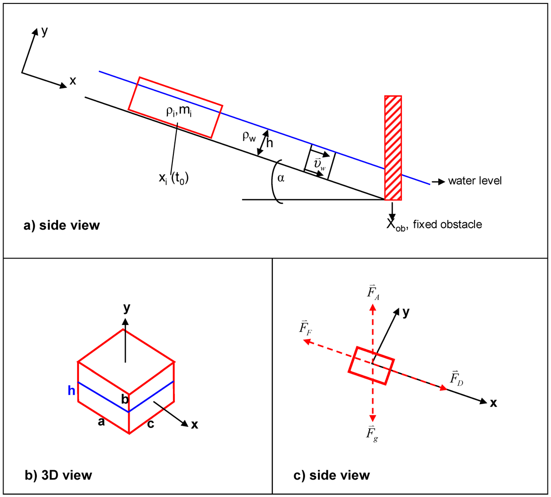
 (after collision) is the only relevant physical damage variable of interest.
 is the drag force,
  is gravity, whereas
  is the force due to friction and
  is the lift force.
 and
and  respectively. The drag force in flow direction is generally expressed as
  , where
  is the drag coefficient,
  is the density of the fluid,
  is the flow depth (or the submerged object depth,
  , once floating occurs) and
  is the width of the object. The force due to friction acting in the opposite direction is expressed as
  , where
  indicates the static or dynamic friction coefficient, depending on whether the object is in motion or not,
  is the acceleration due to gravity,
  are the geometrical parameters of the object and
  is the inclination angle of the plane. The force due to gravity is given by
  , and the lift force that the object is subjected to, is
  (
(  in the case of floating).
 or
or 
 (2)
(2) (3)
(3) or
or 
 (4)
(4) , as
, as , yields the differential equation:
 .
. , we obtain the differential equation for the sliding case:
 (5)
(5) , we obtain its displacement as follows:
 (6)
(6) , can be expressed as:
 (7)
(7) due to collision of object with the fixed obstacle:
 with the deformation depth :
 (8)
(8) and
and  are empirically defined stiffness coefficients, with units [N/m] and [N/m2].
 (9)
(9)
 (10)
(10) (11)
(11) corresponds to a deformation depth, which, once reached, completely destroys the market value of the vehicle.
 . and respectively:
 and
and  remain unaltered during the possible displacement of the bridge deck. Expressed another way, the hydrodynamic loadings at the boundaries of the moving control volume are held constant (compare Figure 2c).
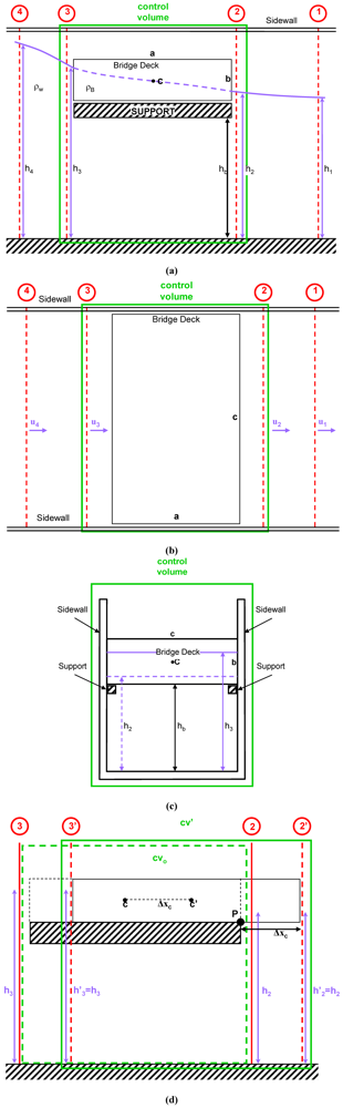
 , which ranges from 0 (stable bridge, no displacement) to a maximum value
  where the equilibrium condition
  (
(  = moments around P) is no longer satisfied:
 (12)
(12) and
and  , which corresponds to the severest loading condition before the bridge starts to be submerged,
  simplifies to:
 (13)
(13) , we assume that the damage corresponds to the reinstatement value of the bridge deck and hence
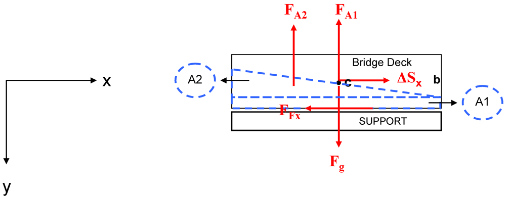
 , entails a comparison between the net hydrodynamic force on the bridge structure
  and the reactive friction force
  .
.  , whereas
  and
and  are the forces acting on the control volume in section 3 and 2 respectively, thus:
  and
and  , therefore:
 , where
  is the force due to gravity,
  and
and  are the lift force components (compare Figure 3):
  and
and  .
. (14)
(14) with
with and
and .
.
 (15)
(15) ,
,  ,
,
 (16)
(16)4. A Formal Cost-Benefit Analysis Framework Based on Dynamic Risk Assessment
4.1. Risk Assessment
 with
with  , and the location
  of each element at risk, assumed to be potentially movable in the general case, their time-varying vulnerability
  can be tracked as outlined, both in theory and practice, in the two preceding sections.
 with
with  reflect the exposure scenarios for the entire object set, and that each exposure scenario has a defined probability
  , we can quantify the time-dependent expected loss
  for an object at risk , for a specified flood scenario and for its exposure configuration as:
 (17)
(17) is the reinstatement value of the considered element and
  is a depreciation coefficient reflecting the element’s obsolescence [19].
 (18)
(18) is the last time-step considered.
 (19)
(19)- a. vertically extending fixed structures (e.g., walls of the buildings) impacted directly by the flood process;
- b. particular superstructures impacted directly (e.g., bridge decks) or indirectly (e.g., roofs) by the flood process.
- c. installations and/or mobile objects (e.g., machines and cars) impacted directly by the flood process.
- d. surfaces (areas) for different land use purposes (e.g., agricultural land, but also parking areas and roads); and
- e. biotic systems (e.g., wood, but also orchards).
 , which can be calculated by:
 (20)
(20) is the required quantity of input to perform the construction workflow unit ; and
  is the unitary of the construction workflow unit .
 , of the equipment components is calculated as follows:
 (21)
(21) is the purchase price;
  is the cost increment from the year of purchase to the year of valuation:
  is the residual economic life (in years) and
  is the economic lifespan (in years).
 ,of a strategy
  ,
,  (compare also Figure 4), can be evaluated by taking the difference between the annual risks (
  and
and  , respectively), calculated by taking the difference of the integrals of the Expected Damage (ED) Probability curves (
  and
and  with
with  indicating the probability of exceeding, mirroring the current situation, mirroring the current situation (subscript
  ) and the hypothesized situation with the implemented strategy respectively (subscript ):
 (22)
(22) (23)
(23) (24) of a mitigation strategy .
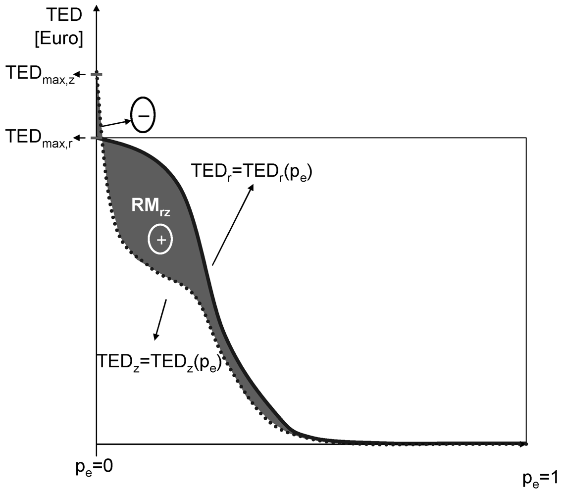
 ). As one may note, for extreme events with
  that tends to zero,
  is larger than
  . This is due to the fact that under extreme loading conditions the elements of the protection system would also be damaged. Structures forming the protection systems feature a “dual nature” [21], as they are designed to mitigate natural process-related hazards, but on the other hand are prone to be damaged throughout their lifecycle by the same processes they should mitigate and their effectiveness thus declines over time.
 associated to the implementation of the strategy can be computed knowing the cost plan -
  over its entire lifecycle of duration
  years.
  , with
  .
. ,associated to the implementation of the strategy can be calculated as:
 (25) and are not available as smooth functions, but have to be obtained by linear interpolation between a finite number of value pairs
  and
and  , respectively) corresponding to the consequences in terms of expected damage of the
  flood hazard under consideration. of a mitigation strategy assuming only a finite number of value pairs (
  and
and  , respectively).
of a mitigation strategy assuming only a finite number of value pairs ( and , respectively).
, respectively).
of a mitigation strategy assuming only a finite number of value pairs ( and , respectively).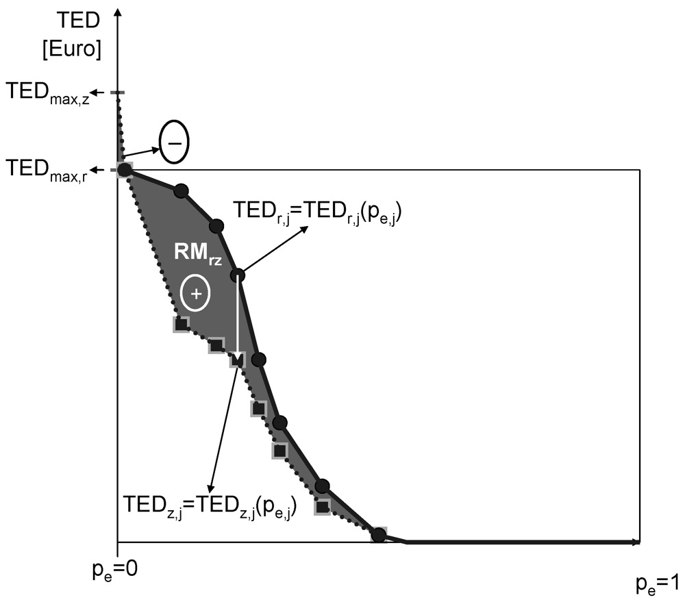
 (26)
(26) (27)
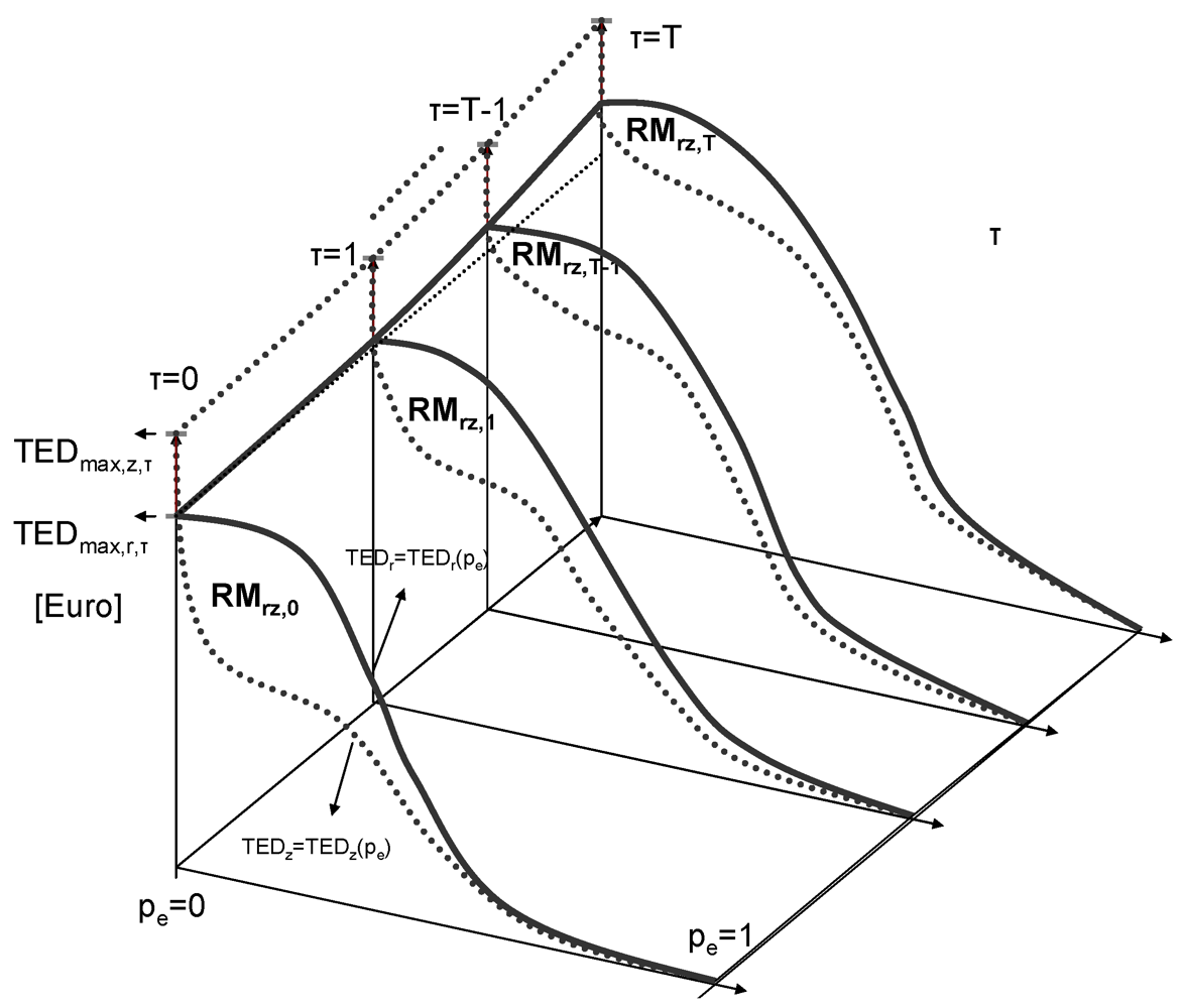
(27) (28) of a mitigation strategy , assuming variability in damage potential and risk mitigation performance through time.
of a mitigation strategy , assuming variability in damage potential and risk mitigation performance through time.
(28) of a mitigation strategy , assuming variability in damage potential and risk mitigation performance through time.
of a mitigation strategy , assuming variability in damage potential and risk mitigation performance through time. , with and (ii) the flow of risk mitigation benefits for each year
  , with . ,associated to the implementation of the strategy z can be calculated as:
 (29)
(29)5. Conclusions
References
- United Nations, Resolutions Adopted by the Conference. Report of the United Nations Conference on Environment and Development: New York, NY, USA, 1993.
- Commission of the European Communities. Directive 2007/60/EC of the European Parliament and of the Council of 23 October 2007 on the Assessment and Management of Flood Risks. Official Journal of the European Union: Luxembourg, 6 November 2007. Available online: http://eur-lex.europa.eu/LexUriServ/LexUriServ.do?uri=OJ:L:2007:288:0027:0034:EN:PDF (accessed on 12 October 2010).
- Commission of the European Communities. Communication from the Commission to the Council, the European Parliament, the European Economic and Social Committee and the Committee of the Regions. Flood risk management eFlood prevention, protection and mitigation. 2004. Available online: http://eur-lex.europa.eu/LexUriServ/LexUriServ.do?uri=COM:2004:0472: FIN:EN:PDF (accessed on 27 October 2010).
- Mazzorana, B.; Fuchs, S. A Conceptual planning tool for hazard and risk management. In Proceedings of the Internationales Symposium Interpraevent, Taipei, Taiwan, 26-30 April 2010; pp. 828–837.
- Merz, B.; Kreibich, H.; Schwarze, R.; Thieken, A. Assessment of economic flood damage. Nat. Hazards Earth Syst. Sci. 2010, 10, 1697–1724. [Google Scholar] [CrossRef]
- Parker, D.J.; Green, C.H.; Thompson, P.M. Urban Flood Protection Benefits: A Project Appraisal Guide; Gower Technical Press: Aldershot, UK, 1987. [Google Scholar]
- Perman, R.; Ma, Y.; Common, M.; Maddison, D.; Mcgilvray, J. Natural Resource and Environmental Economics; Addison-Wesley: Boston, MA, USA, 2011. [Google Scholar]
- Fuchs, S. Mountain Hazard Vulnerability and Risk. Habilitation Thesis, Innsbruck University, Innsbruck, Austria, 2009. [Google Scholar]
- Mazzorana, B.; Comiti, F.; Scherer, C.; Fuchs, S. Developing consistent scenarios to assess flood hazards in mountain streams. J. Environ. Manag. 2011, 94, 112–124. [Google Scholar]
- Mazzorana, B.; Fuchs, S. Fuzzy formative scenario analysis for woody material transport related risks in mountain torrents. Environ. Model. Softw. 2010, 25, 1208–1224. [Google Scholar] [CrossRef]
- Smith, K.; Ward, R. Floods: Physical Processes and Human Impacts; John Wiley & Sons: Chichester, UK, 1998. [Google Scholar]
- Comiti, F.; Mao, L.; Preciso, E.; Picco, L.; Marchi, L.; Borga, M. Large wood and flash floods: Evidences from the 2007 Event in the Davca Basin (Slovenia). In Monitoring, Simulation, Prevention and Remediation of Dense and Debris Flow II; de Wrachien, D., Lenzi, M.A., Brebbia, C.A., Eds.; WIT-Press: Southampton, UK, 2008; pp. 173–182. [Google Scholar]
- Hanley, N.; Spash, C. Cost-Benefit Analysis and the Environment; Edward Elgar: Cheltenham, UK, 1994. [Google Scholar]
- Keiler, M.; Sailer, R.; Jörg, P.; Weber, S.; Zischg, A.; Sauermoser, S. Avalanche risk assessment—A multi-temporal approach, results from Galtür, Austria. Nat. Hazards Earth Syst. Sci. 2006, 6, 637–651. [Google Scholar] [CrossRef]
- Papathoma-Köhle, M.; Kappes, M.; Keiler, M.; Glade, T. Physical vulnerability assessment for alpine hazards: State of the art and future needs. Nat. Hazards 2011, 58, 645–680. [Google Scholar]
- Mileti, D. Disasters by Design; Joseph Henry Press: Washington, DC, USA, 1999. [Google Scholar]
- Daily, J.; Strickland, R.; Daily, J. Crush analysis with under-rides and the coefficient of restitution. In Proceedings of the 24th Annual Special Problems in Traffic Crash Reconstruction; Bloomington, IL, USA: 24-28 April 2006.
- Kruschwitz, L. Investitionsrechnung; 12. Aufl., Oldenbourg Wisssenschaftsverlag GmbH: München, Germany, 2008. [Google Scholar]
- Drees, G.; Paul, W. Kalkulation von Baupreisen; Beuth Verlag: Berlin, Germany, 2011. [Google Scholar]
- Gallerani, V.; Viaggi, D.; Zanni, G. Manuale di Estimo; McGraw-Hill: Milano, Italy, 2011. [Google Scholar]
- Dell’Agnese, A.; Mazzorana, B.; Comiti, F.; von Maravic, P.; D’Agostino, V. Assessing the physical vulnerability of check dams through an empirical damage index. La Houille Blanche. in submit.
- Keiler, M.; Fuchs, S. Berechnetes risiko. Mit sicherheit am rande der gefahrenzone. In Geographische Risikoforschung. Zur Konstruktion verräumlichter Risiken und Sicherheiten; Egner, H., Pott, A., Eds.; Franz Steiner: Stuttgart, Germany, 2010; pp. 51–68. [Google Scholar]
- Renn, O. Concepts of risk: An interdisciplinary review. Part 1: Disciplinary risk concepts. GAIA 2008, 17, 50–66. [Google Scholar]
- Renn, O. Concepts of risk: An interdisciplinary review. Part 2: Integrative approaches. GAIA 2008, 17, 196–204. [Google Scholar]
Mathematical Appendix
 (floating case)
 (sliding case)
 ,
,  ,
,  (A1)
(A1) 
| Case | | | | |
|---|---|---|---|---|
| Floating rigid body |  |  |  |  |
| Sliding rigid body |  |  | |  |
| Bridge |  |  |  |  |
 . In fact one has
 (A2)
(A2)
 By the above equation we have
A1.1. Floating Rigid Body
 and since obviously
  the condition
  is always satisfied. If we assume that the initial velocity of the object is zero and that
  we have
 (A3)
(A3)  (A4)
(A4) A1.2. Free Sliding Rigid Body
 whose sign depends on that of
  since
since  Let
Let  be the critical angle; the sliding condition assures that
  Thus if
  we have as before
 (A5)
(A5)  (A6)
(A6)  setting
  we get
 (A7)
(A7)  (A8)
(A8)  we have
 (A9)
(A9)  (A10)
(A10) A1.3. Bridge

 it can be shown that
  always. Thus, given that the initial velocity of the bridge is zero, setting
  the solution in this case is given by
 (A11)
(A11)  (A12)
(A12) © 2012 by the authors; licensee MDPI, Basel, Switzerland. This article is an open-access article distributed under the terms and conditions of the Creative Commons Attribution license (http://creativecommons.org/licenses/by/3.0/).
Share and Cite
Mazzorana, B.; Levaggi, L.; Formaggioni, O.; Volcan, C. Physical Vulnerability Assessment Based on Fluid and Classical Mechanics to Support Cost-Benefit Analysis of Flood Risk Mitigation Strategies. Water 2012, 4, 196-218. https://doi.org/10.3390/w4010196
Mazzorana B, Levaggi L, Formaggioni O, Volcan C. Physical Vulnerability Assessment Based on Fluid and Classical Mechanics to Support Cost-Benefit Analysis of Flood Risk Mitigation Strategies. Water. 2012; 4(1):196-218. https://doi.org/10.3390/w4010196
Chicago/Turabian StyleMazzorana, Bruno, Laura Levaggi, Omar Formaggioni, and Claudio Volcan. 2012. "Physical Vulnerability Assessment Based on Fluid and Classical Mechanics to Support Cost-Benefit Analysis of Flood Risk Mitigation Strategies" Water 4, no. 1: 196-218. https://doi.org/10.3390/w4010196
APA StyleMazzorana, B., Levaggi, L., Formaggioni, O., & Volcan, C. (2012). Physical Vulnerability Assessment Based on Fluid and Classical Mechanics to Support Cost-Benefit Analysis of Flood Risk Mitigation Strategies. Water, 4(1), 196-218. https://doi.org/10.3390/w4010196