Article

Trade Liberalization and Climate Change: A Computable General Equilibrium Analysis of the Impacts on Global Agriculture

by
Alvaro Calzadilla
1,
Katrin Rehdanz
1,2,* and
Richard S.J. Tol
3,4,5,6
1
Kiel Institute for the World Economy, Hindenburgufer 66, 24105 Kiel, Germany
2
Department of Economics, Christian-Albrechts-University of Kiel, Olshausenstrasse 40, 24118 Kiel, Germany
3
Economic and Social Research Institute, Whitaker Square, Sir John Rogerson’s Quay, Dublin 2, Ireland
4
Institute for Environmental Studies, Vrije Universiteit Amsterdam, De Boelelaan 1087, 1081 HV Amsterdam, The Netherlands
5
Department of Spatial Economics, Vrije Universiteit Amsterdam, De Boelelaan 1105, 1081 HV Amsterdam, The Netherlands
6
Department of Economics, Arts Building, Trinity College, Dublin 2, Ireland
*
Author to whom correspondence should be addressed.
Water 2011, 3(2), 526-550; https://doi.org/10.3390/w3020526
Submission received: 30 March 2011 / Revised: 18 April 2011 / Accepted: 20 April 2011 / Published: 6 May 2011
(This article belongs to the Special Issue Managing Water Resources and Development in a Changing Climate)

Abstract

:
Based on predicted changes in the magnitude and distribution of global precipitation, temperature and river flow under the A1B and A2 scenarios of the Intergovernmental Panel on Climate Change Special Report on Emissions Scenarios (IPCC SRES), this study assesses the potential impacts of climate change and CO2 fertilization on global agriculture, and its interactions with trade liberalization, as proposed for the Doha Development Round. The analysis uses the new version of the GTAP-W model, which distinguishes between rainfed and irrigated agriculture and implements water as an explicit factor of production for irrigated agriculture. Significant reductions in agricultural tariffs lead to modest changes in regional water use. Patterns are non-linear. On the regional level, water use may go up for partial liberalization, and down for more complete liberalization. This is because different crops respond differently to tariff reductions, and because trade and competition matter too. Moreover, trade liberalization tends to reduce water use in water scarce regions, and increase water use in water abundant regions, even though water markets do not exist in most countries. Considering impacts of climate change, the results show that global food production, welfare and GDP fall over time while food prices increase. Larger changes are observed under the SRES A2 scenario for the medium term (2020) and under the SRES A1B scenario for the long term (2050). Combining scenarios of future climate change with trade liberalization, countries are affected differently. However, the overall effect on welfare does not change much.

1. Introduction

Current observations and climate projections suggest that one of the most significant impacts of climate change is likely to be on the hydrological system and hence on river flow and regional water resources [1,2,3]. Climate model simulations suggest that global average precipitation will increase as global temperature rises. As a result, global water availability is expected to increase but at the regional level large differences will occur. At high latitudes and in some wet tropical areas, river flow and water availability are projected to increase. An opposite trend is projected for some dry regions at mid-latitudes and in the dry tropics [2,4]. In many regions, the positive effects of higher annual runoff and total water supply are likely to be offset by the negative effects of changes in precipitation patterns, intensity and extremes, as well as shifts in seasonal runoff. Therefore, the overall global impacts of climate change on freshwater systems are expected to be negative [2]. Since water is essential, the impact of climate change on water resources is potentially one of the most important reasons for concern about unabated greenhouse gas emissions.
Many studies focus on natural science aspects of water availability, but analyses on the economic responses are important as well. Economies and in particular agricultural sectors of some developing countries might be hit particularly hard by a changing climate and a change in water availability putting at risk regional food security and the livelihood conditions for the rural poor. The agricultural sector is by far the largest consumer of water and farmers operate, directly or indirectly, at the world market for agricultural products. As future climate change is expected to modify the regional distribution of freshwater water resources, it could generate new opportunity costs and reverse regional comparative advantages in food production. As a result, regional trade patterns and welfare are expected to change. Regions with reliable water resources may experience positive impacts in food production and exports. At the same time, food-exporting regions may be vulnerable not only to direct climate-induced agricultural damages, but also to positive impacts elsewhere.
Climate variability, especially changes in rainfall patterns, is particularly important for rainfed agriculture. Soil moisture limitations reduce crop productivity and increase the risk of rainfed farming systems. Although the risk of climate variability is reduced by the use of irrigation, irrigated farming systems are dependent on reliable water resources; therefore, they may be exposed to changes in the spatial and temporal distribution of river flow.
One of the few analyses of the impacts of climate-change-induced changes in water resources on agriculture in the context of international trade is Calzadilla et al. [5]. In addition to information on predicted changes in river flows under the IPCC SRES A1B and A2 scenarios from Falloon and Betts [4], they analyze the effects of temperature, precipitation and CO2 fertilization on crop yields. The SRES A1B scenario has relatively little warming while the SRES A2 scenario shows higher levels of greenhouse gas concentration in the atmosphere. The results show that global food production, welfare and GDP fall due to climate change while food prices increase. Larger changes are observed under the SRES A2 scenario for the medium term (2020) and under the SRES A1B scenario for the long term (2050). The results are more pronounced, if irrigation areas respond to water availability as well.
To alleviate the negative effect of climate change, trade could be liberalized to stimulate economic growth, reduce poverty, and expand market access. Agricultural trade liberalization is supposed to be beneficial, if developing countries’ comparative advantages are located in agriculture. Depending on the scenario chosen, most studies find a positive economic effect of agricultural trade liberalization for developing countries [6,7].
Changes in tariffs or subsidies for agricultural goods involve regional as well as global adjustments in the production of the goods in question but have effects on other markets, such as factor input markets, as well. Water is one production factor in agriculture. Therefore, trade liberalization in agriculture might enhance or alleviate problems related to water use and water availability. To our knowledge, this is the first analysis of the interaction of trade liberalization and climate change using a multi-region, multi-sector general equilibrium model.
Most of the current analyses on agricultural trade liberalization pay no attention to the impact on water use and problems related to water availability. Some authors have looked at the potential impact on sustainable development in developing countries including water as an environmental service. George and Kirkpatrick [8] argue that further trade liberalization would lead to an improved overall availability of water through increased efficiency in all developing countries [9]. Their study does not distinguish between different developing countries nor is a quantitative assessment provided. Other studies related to water issues investigate the implications of the General Agreement on Trade in Services (GATS) negotiations on service trade liberalization on water management and the ability of governments to regulate water services (see e.g., [10,11]). All these analyses are qualitative assessments not based on economic models. Berrittella et al. [12] is an exception. They use a global computable general equilibrium (CGE) model including water resources (GTAP-W, Version 1) to analyze the economic impact of hypothetical Doha-like liberalization of agricultural trade on water use. The Doha Development Agenda [13], launched in 2001, is meant to improve the situation for developing countries, but is subject to seemingly interminable delays.
This paper differs from previous work in three ways. First, we use the Version 2 of the GTAP-W model. See Calzadilla et al. [14,15] for a detailed description of the model. Second, we base our analysis on future scenarios of climate change for two time periods (2020 and 2050) as described in Calzadilla et al. [5]. They investigate the effect of climate change on water use and water availability but ignore the impact that trade liberalization could have on the economy. Based on their results we, thirdly, investigate how trade patterns would change if trade of agricultural products were liberalized. Similar to Berrittella et al. [12], we assume a hypothetical Doha-like liberalization but we introduce water as an explicit factor of production.
The remainder of the paper is organized as follows: Section 2 briefly presents the model used. Section 3 lays down the simulation scenarios. Section 4 discusses the results and Section 5 concludes.

2. The GTAP-W Model (Version 2)

Economic models of water use have generally been applied to look at the direct effects of water policies, such as water pricing or quantity regulations, on the allocation of water resources. In order to obtain insights from alternative water policy scenarios on the allocation of water resources, partial and general equilibrium models have been used. While partial equilibrium analysis focus on the sector affected by a policy measure assuming that the rest of the economy is not affected, general equilibrium models consider other sectors or regions as well to determine the economy-wide effect; partial equilibrium models tend to have more detail. Most of the studies using either of the two approaches analyze pricing of irrigation water only (for an overview of this literature see [16]). Rosegrant et al. [17] use the IMPACT model to estimate demand and supply of food and water to 2025. Fraiture et al. [18] extend this to include virtual water trade, using cereals as an indicator. Their results suggest that the role of virtual water trade is modest. While the IMPACT model covers a wide range of agricultural products and regions, other sectors are excluded; it is a partial equilibrium model.
Studies of water use using general equilibrium approaches are generally based on data for a single country or region assuming no effects for the rest of the world of the implemented policy (for an overview of this literature see [14,19]). All of these CGE studies have a limited geographical scope. Berrittella et al. [20] and Calzadilla et al. [14,15] are exceptions, using GTAP-W, a static multi-region world CGE model.
With GTAP-W, it is possible to assess the systemic general equilibrium effects of climate change impacts and trade liberalization on global agriculture. The model is a further refinement of the GTAP model [21,22], and is based on the version modified by Burniaux and Truong [23,24] as well as on the previous GTAP-W model introduced by Berrittella et al. [20]. For a more detailed description of the model see [14].
Unlike Version 1 [20], Version 2 of the GTAP-W model [14,15], used here, distinguishes between rainfed and irrigated agriculture. In Version 1 of the GTAP-W model, substitution between intermediate inputs and value-added for the production function of tradable goods and services was not possible. As a consequence, a price-induced drop in water demand did not imply an increase in any other input. Water was a technology of land, that is, water was assumed to modify soil moisture and hence the productivity of land. In Version 2, water is an explicit factor of production in irrigated agriculture and accounts for substitution possibilities between water and other primary factors.
The new GTAP-W model is based on the GTAP Version 6 database, which represents the global economy in 2001, and on the IMPACT 2000 baseline data. The model has 16 regions and 22 sectors, seven of which are in agriculture [25]. However, the most significant change and principal characteristic of Version 2 of the GTAP-W model is the new production structure, in which the original land endowment in the value-added nest has been split into pasture land (grazing land used by livestock) and land for rainfed and for irrigated agriculture. The last two types of land differ as rainfall is free but irrigation development is costly. As a result, land equipped for irrigation is generally more valuable as yields per hectare are higher. To account for this difference, we split irrigated agriculture further into the value for land and the value for irrigation. The value of irrigation includes the equipment but also the water necessary for agricultural production. In the short-run irrigation equipment is fixed, and yields in irrigated agriculture depend mainly on water availability. The tree diagram in Figure A1 in Annex A represents the production structure.
Land as a factor of production in national accounts represents “the ground, including the soil covering and any associated surface waters, over which ownership rights are enforced” [26]. In order to include water as a factor of production in the GTAP data and model, we split for each region and each crop the value of land included in the GTAP social accounting matrix into the value of rainfed land and the value of irrigated land in proportion to its contribution to total production. The value of pasture land is derived from the value of land in the livestock breeding sector.
In the next step, we split the value of irrigated land into the value of land and the value of irrigation using the ratio of irrigated yield to rainfed yield. These ratios are based on IMPACT data. The numbers indicate how valuable irrigated agriculture is compared to rainfed agriculture. The magnitude of additional yield differs not only with respect to the region but also to the crop. On average, producing rice using irrigation is relatively more productive than using irrigation for growing oil seeds, for example. On average, regions like South America seems to grow relatively more using irrigation instead of rainfed agriculture compared to countries in North Africa or Sub-Saharan Africa.
The procedure we described above to introduce the four new endowments (pasture land, rainfed land, irrigated land and irrigation) allows us to avoid problems related to model calibration. In fact, since the original database is only split and not altered, the original regions’ social accounting matrices are balanced and can be used by the GTAP-W model to assign values to the share parameters of the mathematical equations. For detailed information about the social accounting matrix representation of the GTAP database see [27].
As in all CGE models, the GTAP-W model makes use of the Walrasian perfect competition paradigm to simulate adjustment processes. Industries are modeled through a representative firm, which maximizes profits in perfectly competitive markets. The production functions are specified via a series of nested constant elasticity of substitution functions (CES) (Figure A1). Domestic and foreign inputs are not perfect substitutes, according to the so-called ‘‘Armington assumption’’, which accounts for product heterogeneity and non-tariff trade barriers.
A representative consumer in each region receives income, defined as the service value of national primary factors (natural resources, pasture land, rainfed land, irrigated land, irrigation, labour and capital). Capital and labour are perfectly mobile domestically, but immobile internationally. Pasture land, rainfed land, irrigated land, irrigation and natural resources are imperfectly mobile. While perfectly mobile factors earn the same market return regardless of where they are employed, market returns for imperfectly mobile factors may differ across sectors. The national income is allocated between aggregate household consumption, public consumption and savings. The expenditure shares are generally fixed, which amounts to saying that the top level utility function has a Cobb-Douglas specification. Private consumption is split in a series of alternative composite Armington aggregates. The functional specification used at this level is the constant difference in elasticities (CDE) form: a non-homothetic function, which is used to account for possible differences in income elasticities for the various consumption goods. A money metric measure of economic welfare, the equivalent variation, can be computed from the model output.
In the original GTAP model, land is combined with natural resources, labor and the capital-energy composite in a value-added nest. In our modeling framework, we incorporate the possibility of substitution between land and irrigation in irrigated agricultural production by using a nested constant elasticity of substitution function (Figure A1). The procedure how the elasticity of factor substitution between land and irrigation (σLW) was obtained is explained in detail in [14,15]. Next, the irrigated land-water composite is combined with pasture land, rainfed land, natural resources, labor and the capital-energy composite in a value-added nest through a CES structure.
The IMPACT model [17] provides detailed information on green water use in rainfed production (defined as effective rainfall); and both green and blue water use in irrigated production (blue water or irrigation is defined as the water diverted from water systems) [28]. In the GTAP-W benchmark equilibrium, water used for irrigation is supposed to be identical to the volume of blue water used for irrigated agriculture in the IMPACT model. An initial sector and region specific shadow price for irrigation water can be obtained by combining the social accounting matrix information about payments to factors of production with the volume of water used in irrigation estimated by the IMPACT model. In the model only irrigation water has a price. In contrast, any rain that falls directly on a crop, whether rainfed or irrigated, is not priced. Instead, the amount of rain that falls on a crop is modeled exogenously in the GTAP-W model using information from IMPACT.
The distinction between rainfed and irrigated agriculture within the production structure of the GTAP-W model allows us to study expected physical constraints on water supply due to, for example, climate change. In fact, changes in rainfall patterns can be exogenously modeled in GTAP-W by changes in the productivity of rainfed and irrigated land. In the same way, water excess or shortages in irrigated agriculture can be modeled by exogenous changes to the initial irrigation water endowment.

3. Design of Model Experiments

Our model experiments are based on future impacts of climate change on agriculture at two time periods: 2020 and 2050 [29]. In a first step, information on the future benchmark equilibria under normal climate conditions (omitting climate change) is needed. How to find a hypothetical general equilibrium state in the future imposing forecasted values for some key economic variables in the initial calibration dataset is described in [5]. Since the GTAP-W model is a static multi-region world CGE model we are not able to look at dynamic effects over time but rather compare different points in time.
The current baseline data and future baseline simulations under normal climate conditions are shown in Annex B. These baselines are based on the IMPACT model [17]. Compared to the 2000 baseline data (Table B1) a growth in both crop harvested area as well as crop productivity under normal climate conditions (assuming no climate change) is projected for 2020 and 2050 (Table B2). For 2020 and 2050 respectively, global agricultural area increases by 1.1% and 2.8% while production rises by 32.8% and 91.7%.
To investigate the impact of climate change on global agriculture Calzadilla et al. [5] use information on key climate variables, which includes temperature, precipitation as well as river flow. Their analysis also includes the CO2 fertilization effect. Predicted changes in the magnitude and distribution of global temperature, precipitation and river flow are based on [4]. They used the Hadley Centre Global Environmental Model, including a dynamic river routing model (HadGEM1-TRIP), to simulate changes in temperature, precipitation and river flow over the next century and under the IPCC SRES A1B and A2 scenarios [30]. Crop yield response to temperature and precipitation are taken from [31]. They used the CERES and SOYGRO crop models to analyze crop yield responses to arbitrary incremental changes in temperature (+2 °C and +4 °C) and precipitation (+/−20%). The study was carried out in 18 countries worldwide and uses common crop growth models and methodology.
River flow is a useful indicator of freshwater availability for agricultural production. Irrigated agriculture relies on the availability of irrigation water from surface and groundwater sources, which depend on the seasonality and interannual variability of river flow. Therefore, river flow limits a region’s water supply and hence constrains its ability to irrigate crops. Regional changes in river flow are related to regional changes in water supply by the runoff elasticities of water supply estimated by [32].
The CO2 fertilization effect on crops yields is based on information presented by [33]. They report yield response ratios for C3 and C4 crops to elevated CO2 concentrations in the three major crop models (CERES, EPIC and AEZ). In this analysis, we use the average crop yield response of the three crop models to the CO2 concentrations in 2020 and 2050 for the IPCC SRES A1B and A2 scenarios.
Future climate change would modify regional water endowments and soil moisture, and in response the distribution of harvested land would change. Therefore, we include a land use scenario, which explores possible shifts in the geographical distribution of irrigated agriculture. It assumes that irrigated areas could expand in regions with higher water supply. Vice versa, irrigated farming can become unsustainable in regions subject to water shortages.
Based on the impact of climate change on agricultural production, we analyze in a next step if trade liberalization policies would help to alleviate the negative effect of climate change. To better be able to single out the effect of trade liberalization on agricultural production, we also analyze the impact of reductions in trade barriers ignoring the effect of climate change. As indicated above, the scenarios are based on a hypothetical Doha-like liberalization of agricultural trade.
As the Doha negotiations are still ongoing (at a very slow pace), the modalities of the possible agreement are uncertain. It is clear that the parties involved have very different interests. Agricultural exporters aim for open foreign markets and reductions in distorting subsidies elsewhere. Industrial exporters in emerging economies want to remain protected. Countries with comparative advantages in services wish the GATS negotiations would be successful in reducing national regulatory in services. Therefore, any analysis investigating scenarios of trade liberalization have to take all three aspects into account. However, as our study focuses on trade liberalization in agriculture, we account for liberalization in non-agricultural sectors, but vary the levels of liberalization for the agricultural sectors only. The cut in tariffs for products in the non-agricultural sectors is 25%.
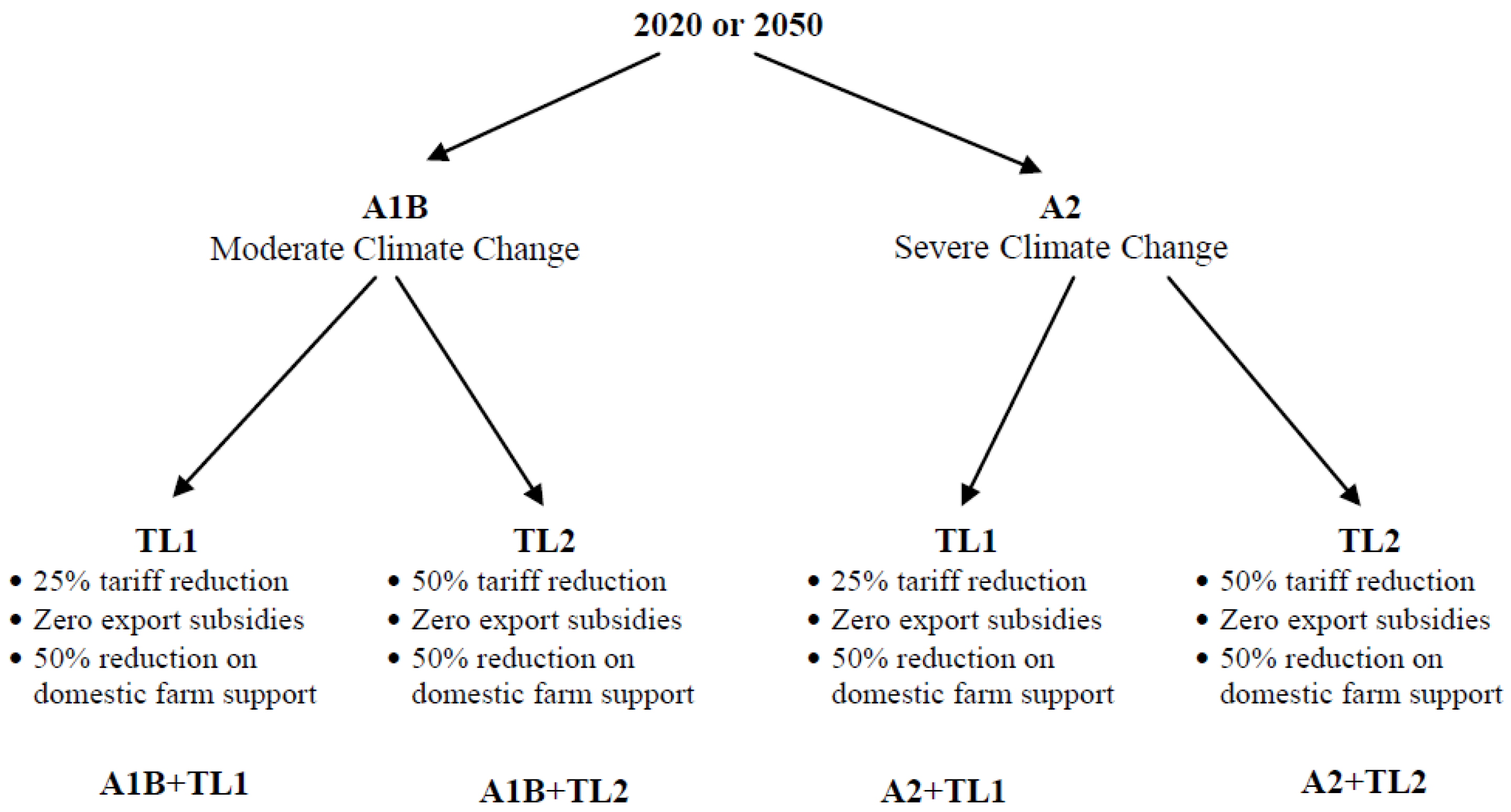
In Scenario 1, a 25% tariff reduction is chosen for all agricultural sectors (TL1). In addition, we assume zero export subsidies and a 50% reduction in domestic farm support. Scenario 2 is a variant of Scenario 1: tariffs are reduced by 50% (TL2). According to the negotiations so far, export subsidies will be phased out over a few years. Tariff reductions will also not be implemented at once but phased in. To account for this procedure, we designed our above described scenarios for the year 2020 and 2050.
In total we have sixteen different scenarios including two climate scenarios (A1B and A2), for two future time periods (2020 and 2050) and two trade liberalization scenarios (TL1 and TL2). See Figure 1. Note that the no climate change scenarios are not displayed.
Figure 1. Structure of climate change scenarios.
Water 03 00526 g001

4. Simulation Results

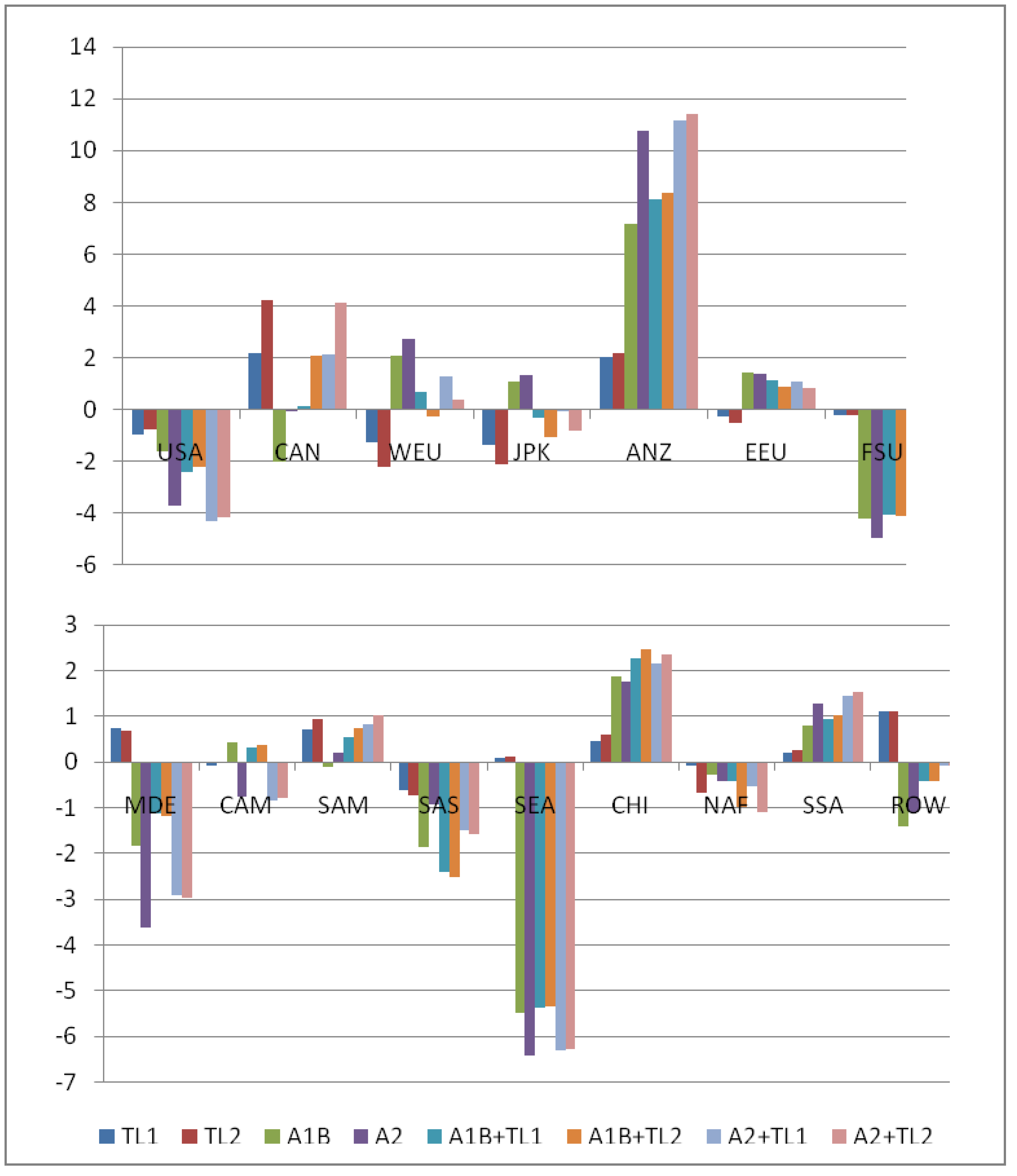
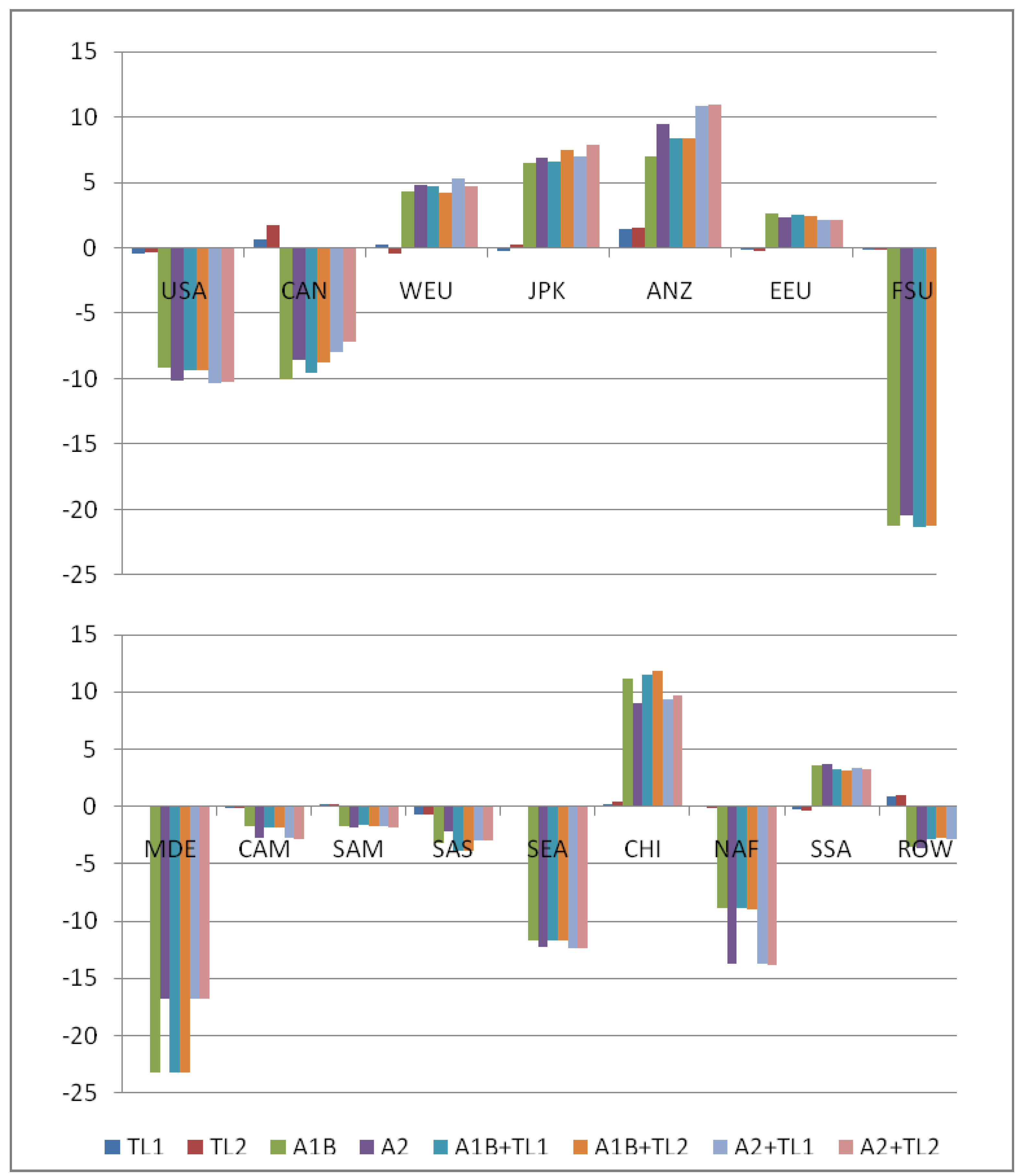
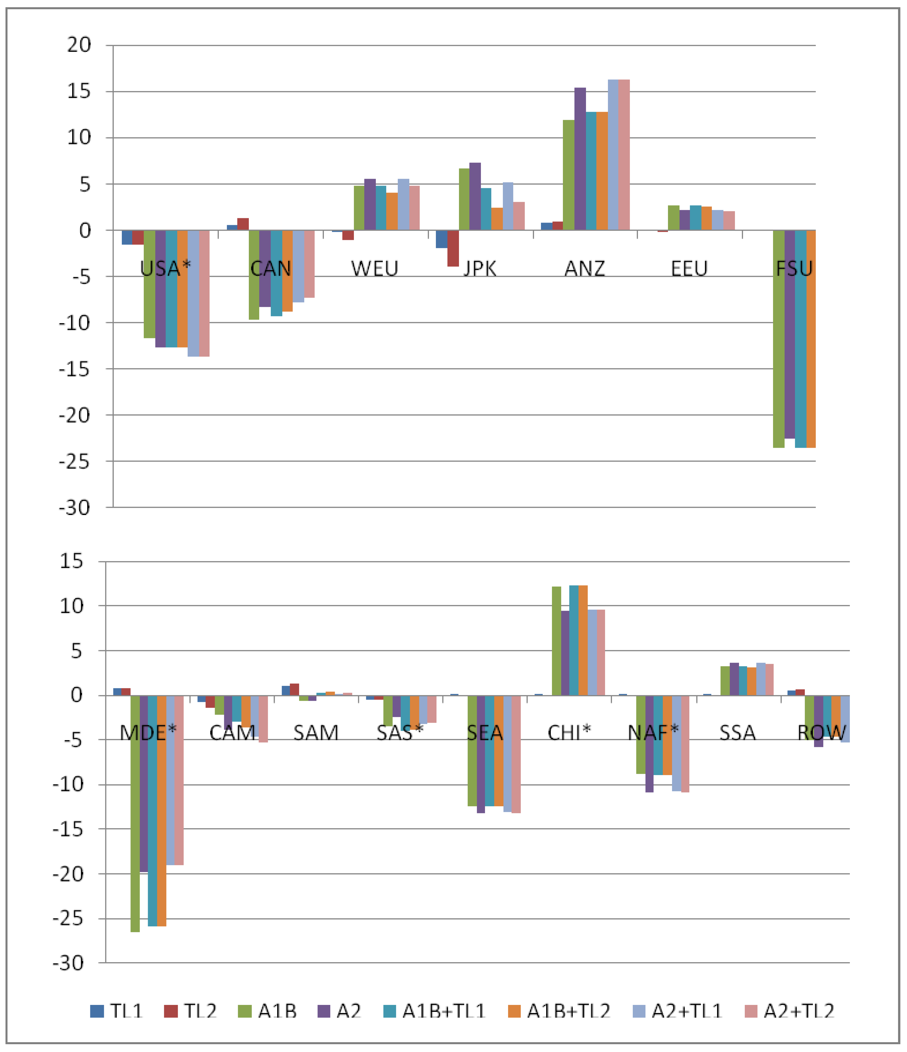
Trade liberalization only (TL1 and TL2) would have a limited effect on global production of agricultural goods (Figure 2 and Figure 3) [34]. On the regional level, the effect is different but the numbers are small. Some regions expand production (particularly Canada (CAN), Australia and New Zealand (ANZ)), while others reduce production (in 2020 particularly Western Europe (WEU), Japan and South Korea (JPK) and in 2050 particularly South Asia (SAS) and the USA). In most of the developing regions the effect of trade liberalization on agricultural production would be positive except for Central America (CAM), South Asia (SAS). For North Africa (NAF) the sign of the effect depends on the liberalization scenario chosen and the time period. For WEU and JPK the effect in 2050 is mixed as well. The relationship between trade liberalization and agricultural production is complex. Current tariffs vary widely between crops and between regions, also relative to the costs of production. Uniform cuts in nominal tariffs, as investigated here, would therefore have a non-uniform impact.
Figure 2. Change in agricultural production in 2020 (in %) relative to the baseline.
Water 03 00526 g002
Note: Developed regions (top panel) and developing regions (bottom panel).
The effect of climate change is a reduction in global agricultural production (A1B and A2). The decrease is more pronounced in 2050 and for the A2 scenario. While in 2020 only irrigated production decreases, rainfed production falls as well in 2050 (not shown) [35]. On a regional level, the drop in production is particularly pronounced in regions such as Southeast Asia (SEA), the Middle East (MDE) and the Former Soviet Union (FSU) as well as the USA while in other regions including Australia and New Zealand (ANZ), Western Europe (WEU) and China (CHI) more is produced. Over time more regions are negatively affected but in some regions the effect of more severe climate change (A2) is less negative compared to more moderate changes (A1B).
Figure 3. Change in agricultural production in 2050 (in %) relative to the baseline.
Water 03 00526 g003
Note: Developed regions (top panel) and developing regions (bottom panel).
Climate change plus trade liberalization changes this pattern for some countries and world regions. In 2020 the impact on production is negative for Western Europe (WEU), the USA, South Asia (SAS), Japan and South Korea (JPK), it is positive (or less negative) for Canada (CAN), South America (SAM), China (CHI) and Sub-Saharan Africa (SSA). In 2050 the situation is different also with respect to the two climate scenarios. Here the effect of trade liberalization on production is negligible. The results are dominated by impacts of climate change.
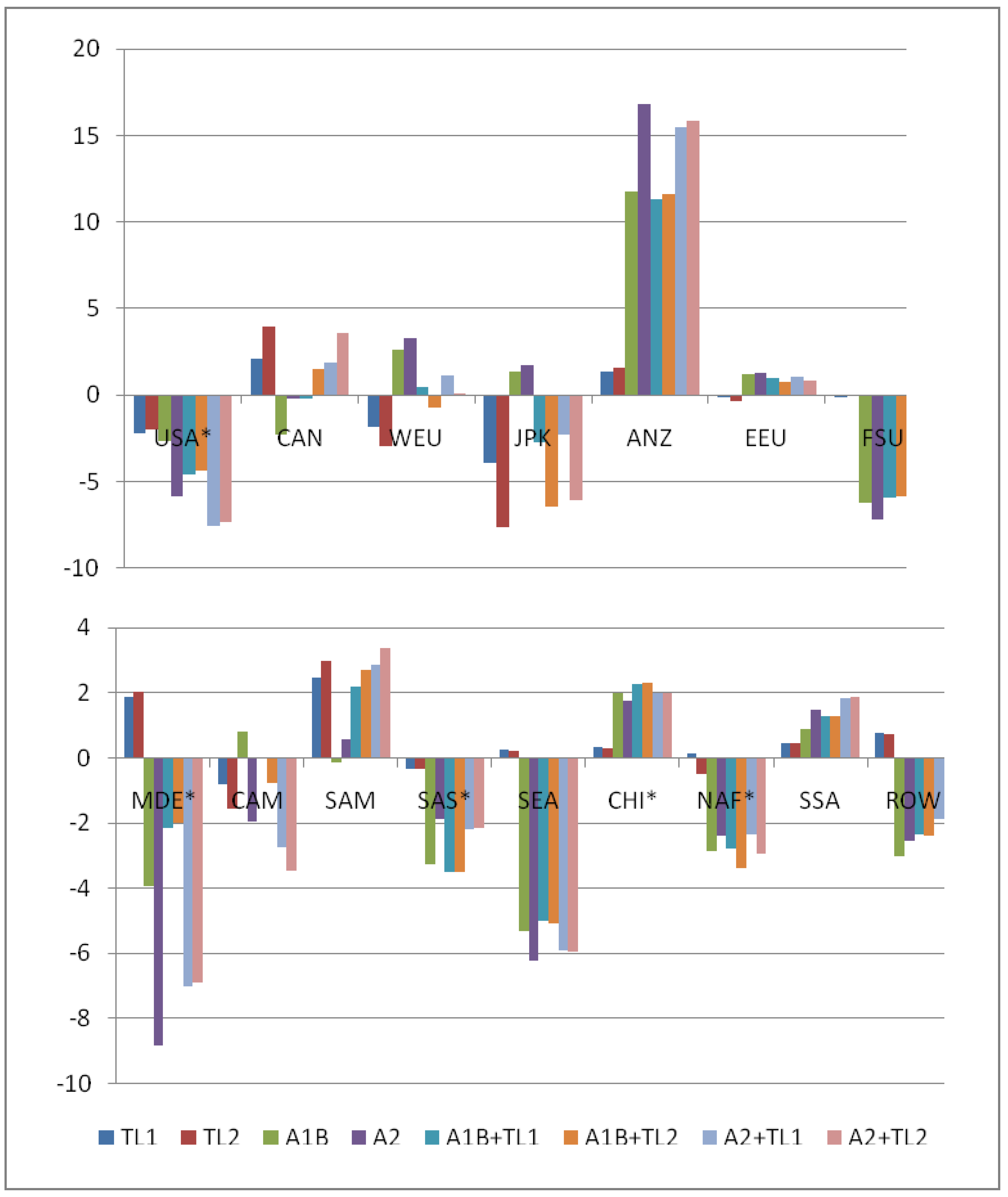
Figure 4 and Figure 5 show the effect of the different scenarios on water use. Qualitatively, the pattern is the same as for agricultural production (Figure 2 and Figure 3) [36]. Trade liberalization only (TL1 and TL2) would imply an increase in water use in Canada (CAN), Australia and New Zealand (ANZ); and a reduction in the USA, Western and Eastern Europe (WEU), Japan and South Korea (JPK), and the former Soviet Union (FSU). In developing regions trade liberalization would mainly lead to higher levels of water use. However, in later years some of these regions would see an increase in water use for a partial liberalization, but a decrease for a more complete liberalization. In all cases, changes in water use due to trade liberalization are less than 10%.
Figure 4. Change in agricultural water use in 2020 relative to baseline (in %).
Water 03 00526 g004
Note: Developed regions (top panel) and developing regions (bottom panel). Regions where overdrafting of groundwater aquifers occurs are denoted by an asterisk (*).
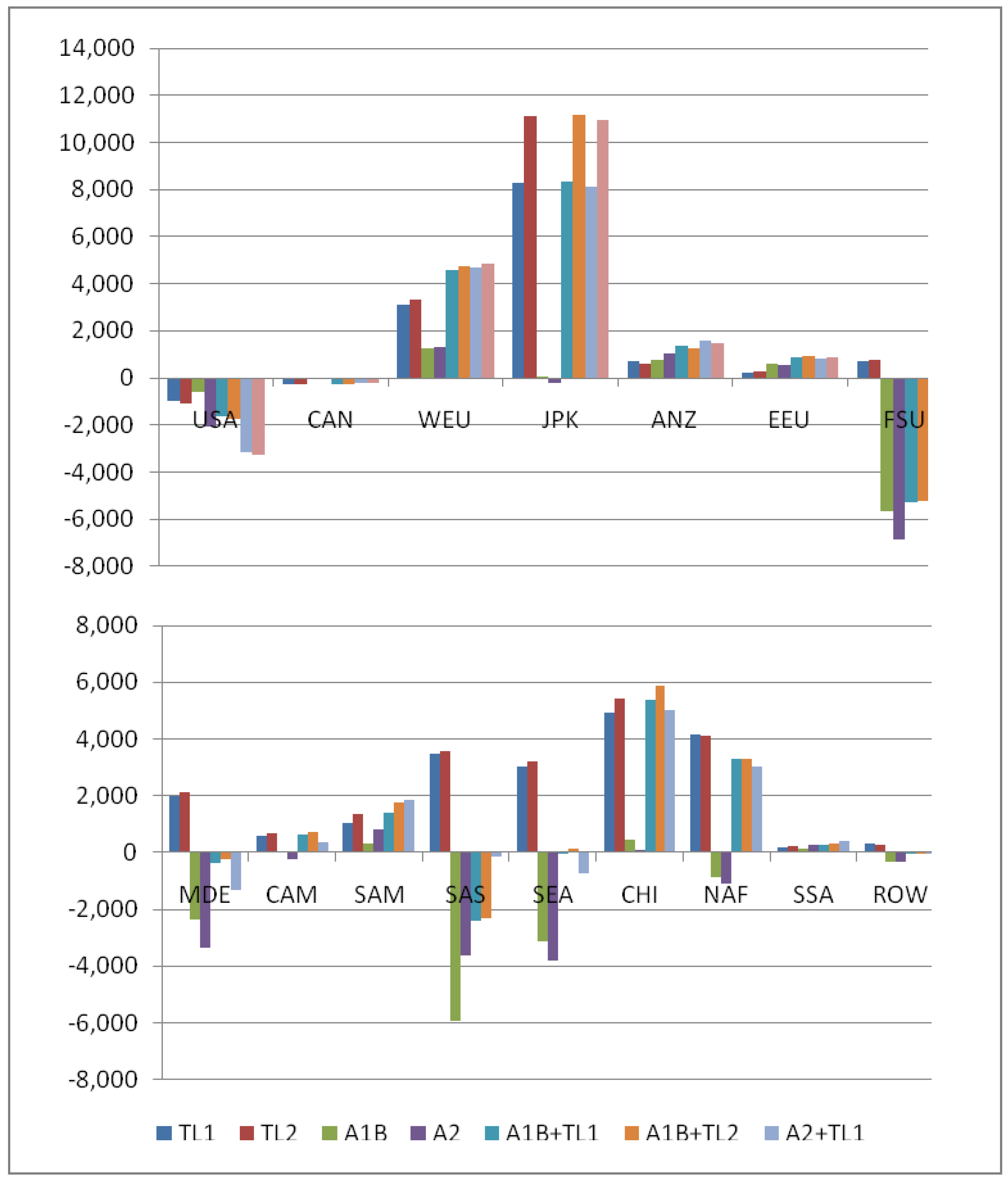
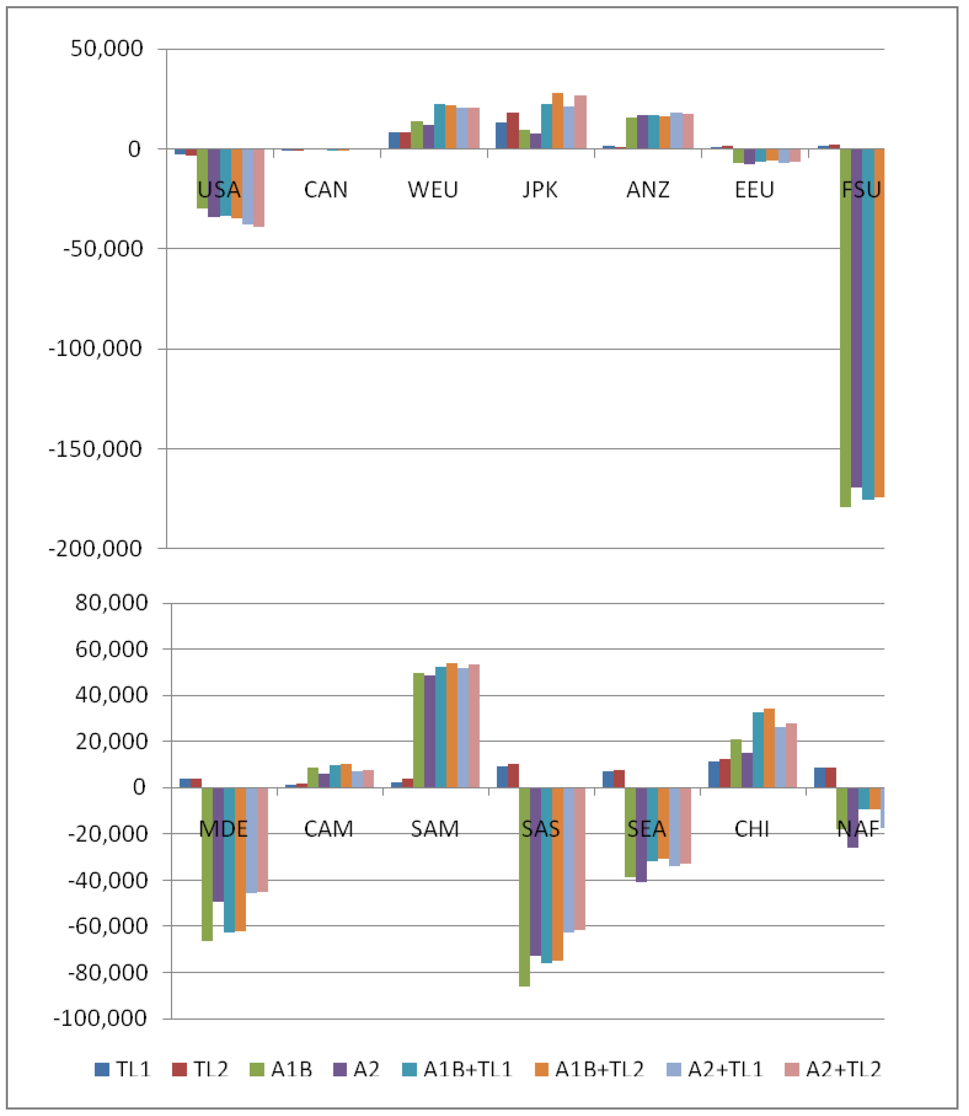
Figure 6 and Figure 7 show the impact of climate change and trade liberalization on welfare. Trade liberalization has a positive effect on welfare of US$31 billion (bln) in 2020 and US$67 bln in 2050 for the 25% cut in tariffs (TL1). An extra 25% tariff cut further increases welfare by US$4 bln in 2020 and US$10 bln in 2050 (TL2). As expected, the first cuts have the greatest benefit. On the regional level, the effect is almost always positive, except for the USA and Canada. The impact of climate change on welfare is negative; up to US$18 bln in 2020 and US$ 283 bln in 2050.
Figure 5. Change in agricultural water use in 2050 relative to baseline (in %).
Water 03 00526 g005
Note: Developed regions (top panel) and developing regions (bottom panel). Regions where overdrafting of groundwater aquifers occurs are denoted by an asterisk (*).
The impact of trade liberalization varies with climate change, as regions are affected differently. In 2020, the impact of climate change is small and the effect of trade liberalization outweighs the negative impact of climate change; the combined effect is an increase of up to US$20 bln. However, in 2050 the negative impact of climate change dominates the positive effect of trade liberalization; welfare decreases by up to US $214 bln. Comparing the individual effects of trade liberalization (TL1, TL2) and climate change (A1B, A2) to the combined effect, welfare decreases less (up to US$2 bln (AB1 + TL1) or up to US$4 bln (A1B + TL2)). The assumption is as follows. Trade liberalization would make it easier to substitute domestic food production for import—and hence make it easier to adapt to climate change.
Figure 6. Change in welfare for 2020 (in Mio USD) relative to the baseline.
Water 03 00526 g006
Note: Developed regions (top panel) and developing regions (bottom panel).
The results presented in Figure 6 and Figure 7 indicate that regions are affected very differently. In the USA, climate change has a negative impact on welfare in the first time period but the effect of trade liberalization is worse, irrespective of the climate scenario. For the Former Soviet Union the situation is more severe. The opposite is true for Western Europe and in particular for China, Japan and South Korea as well as for Northern Africa. However differences exist with respect to time. In 2050 the impact of climate change dominates and the effect of trade liberalization on welfare is minor for all regions.
Figure 7. Change in welfare for 2050 (in Mio USD) relative to the baseline.
Water 03 00526 g007
Note: Developed regions (top panel) and developing regions (bottom panel).

5. Discussion and Conclusions

We use a global computable general equilibrium model including water resources (GTAP-W, Version 2) to assess impacts of climate change and trade liberalization on global agriculture. We find that trade liberalization has a small effect on agricultural production and on water use. Water use for some crops and some regions goes up, and it goes down for other crops and regions. Signs may switch between a modest liberalization and more substantial trade liberalization (e.g., for China and Southeast Asia). Trade liberalization reduces water use in places where it is scarce (including e.g. the Middle East, Northern Africa), and increases water use in places where it is more abundant. Overall and for most regions of the world, the effect of trade liberalization on welfare is positive.
The impact of climate change on global agriculture is much more pronounced. Agricultural production and water use decrease, as does global welfare. On a regional level, the drop in production is particularly pronounced in the Middle East, North Africa, South-East Asia as well as the USA and Canada. Production increases in China, Japan and South Korea, Western Europe, and Australia and New Zealand. The net effect of these positive and negative changes is negative: global welfare decreases by up to US$ 283 bln (0.29% of GDP).
Trade liberalization increases the depth of the market and thus the capacity to adapt to climate change. As a result, in 2050, trade liberalization reduces the negative impact of climate change on welfare, albeit by less than 2%. In 2020, however, trade liberalization shifts production to areas that are more susceptible to climate change.
In summary, significant reductions in agricultural tariffs lead to modest changes in regional water use. Patterns are non-linear. On the regional level water use may go up for partial liberalization, and down for more complete liberalization. This is because different crops respond differently to tariff reductions, and because trade and competition matter too. Moreover, trade liberalization tends to reduce water use in water scarce regions, and increase water use in water abundant regions, even though water markets do not exist in most countries. The welfare impact of climate change is substantially larger than the welfare impact of tariff cuts. Trade liberalization reduces the negative impacts of climate change, but only slightly.
A direct comparison of the results of our study on the impact of climate change and trade liberalization to those of others is difficult since no other study exists using a global CGE approach. Earlier studies, based on other approaches and using different data, tend to find stronger impacts of climate change on agriculture [37,38]. In general, such studies have (1) a more regional focus and do not aim for a global analysis and (2) omit implications of international trade. In addition, the type of crop model chosen and the coverage of changes in the climate and hydrological system are likely to influence the results. Earlier studies are based on changes in temperature and precipitation while our analysis uses additional information on changes in river flow and CO2 fertilization rates.
Several limitations apply to the above results. The model is static. A dynamic model may find larger effects of trade liberalization and climate change with further specialization through capital stock adjustments. The deterministic nature of our model is another limitation. In the spirit of Tyers and Anderson [39], more liberal agricultural trade should allow for smoother adjustment to shocks, at least on a global basis. This is a principal argument for a more liberal agricultural trade regime in the context of climate change but is not considered. The limited disaggregation of crops and regions may hide larger shifts in agricultural production and water use due to trade liberalization. The importance of these factors will need to be tested with a future version of the current model and with other models. Our scenarios on climate change use information on temperature, precipitation river flow based on regional averages. We do not take into account that precipitation and river flow might increase in some water basins and decrease in others within the same region. These local effects are averaged out. Also, we use annual average temperature, precipitation and river flow data; we consider neither changes in the seasonality of river flow nor extreme events. We do not take into account the effects of groundwater depletion. In addition, uncertainty exists especially regarding the future distribution of precipitation which has implications for agricultural production. Our analysis is limited to the use of results of one such study [4]. These issues are deferred to future research.

References and Notes

  1. IPCC. Climate Change 2001: Impacts, Adaptation and Vulnerability; Contribution of Working Group II to the Third Assessment Report of the IPCC; McCarthy, J.J., Canziani, O.F., Leary, N.A., Dokken, D.J., White, K.S., Eds.; Cambridge University Press: Cambridge, UK, 2001. [Google Scholar]
  2. Climate Change and Water; Technical Paper of the Intergovernmental Panel on Climate Change; Bates, B.C.; Kundzewicz, Z.W.; Wu, S.; Palutikof, J.P. (Eds.) IPCC Secretariat: Geneva, Switzerland, 2008.
  3. IPCC. Climate Change 2007: Impacts, Adaption and Vulnerability; Contribution of Working Group II to the Fourth Assessment Report of the IPCC; Parry, M.L., Canziani, O.F., Palutikof, J.P., van der Linden, P.J., Hanson, C.E., Eds.; Cambridge University Press: Cambridge, UK, 2007. [Google Scholar]
  4. Falloon, P.D.; Betts, R.A. The impact of climate change on global river flow in HadGEMI simulations. Atmos. Sci. Let. 2006, 7, 62–68. [Google Scholar] [CrossRef]
  5. Calzadilla, A.; Betts, R.A.; Falloon, P.D.; Rehdanz, K.; Tol, R.S.J. Climate Change Impacts on Global Agriculture; Kiel working paper No. 1617; Kiel Institute for the World Economy: Kiel, Germany, 2010. [Google Scholar]
  6. Anderson, K.; Martin, W.; van der Mensbrugghe, D. Would multilateral trade reform benefit Sub-Saharan Africans? J. Afr. Econ. 2006, 15, 626–670. [Google Scholar]
  7. Francois, J.; van Meijl, H.; van Tongeren, F. Trade liberalization in the Doha development round. Econ. Policy 2005, 42, 349–391. [Google Scholar]
  8. George, C.; Kirkpatrick, C. Trade and development: Assessing the impact of trade liberalization on sustainable development. J. World Trade 2004, 38, 441–469. [Google Scholar]
  9. They mention that regulatory and subsidy frameworks are critical.
  10. Watson, C. Trade and Water—The Role of WTO and GATS: Opening the Water Sector to New Service Providers; WaterAid: London, UK, 2004. [Google Scholar]
  11. Kirkpatrick, C.; Parker, D. Domestic regulation and the WTO: The case of water services in developing countries. World Econ. 2005, 28, 1491–1508. [Google Scholar] [CrossRef]
  12. Berrittella, M.; Rehdanz, K.; Tol, R.S.J.; Zhang, Y. The impact of trade liberalisation on water use: A computable general equilibrium analysis. J. Econ. Integr. 2008, 23, 631–655. [Google Scholar] [CrossRef]
  13. Fergusson, I.F. World Trade Organization Negotiations: The Doha Development Agenda; Congressional Research Service: Washington, DC, USA, 2008. Available online: http://www.nationalaglawcenter.org/assets/crs/RL32060.pdf (accessed on 18 January 2008).
  14. Calzadilla, A.; Rehdanz, K.; Tol, R.S.J. The economic impact of more sustainable water use in agriculture: A computable general equilibrium analysis. J. Hydrol. 2010, 384, 292–305. [Google Scholar] [CrossRef]
  15. Calzadilla, A.; Rehdanz, K.; Tol, R.S.J. Water scarcity and the impact of improved irrigation management: A computable general equilibrium analysis. Agr. Econ. 2011, 42, 305–323. [Google Scholar] [CrossRef]
  16. Johansson, R.C.; Tsur, Y.; Roe, T.L.; Doukkali, R.; Dinar, A. Pricing irrigation water: A review of theory and practice. Water Policy 2002, 4, 173–199. [Google Scholar] [CrossRef]
  17. Rosegrant, M.W.; Cai, X.; Cline, S.A. World Water and Food to 2025: Dealing with Scarcity; International Food Policy Research Institute: Washington, DC, USA, 2002. [Google Scholar]
  18. De Fraiture, C.; Cai, X.; Amarasinghe, U.; Rosegrant, M.; Molden, D. Does International Cereal Trade Save Water? The Impact of Virtual Water Trade on Global Water Use; Comprehensive Assessment of Water Management in Agriculture, Research Report 4; International Water Management Institute: Colombo, Sri Lanka, 2004. [Google Scholar]
  19. Dudu, H.; Chumi, S. Economics of Irrigation Water Management: A Literature Survey with Focus on Partial and General Equilibrium Models; Policy research working paper 4556; World Bank: Washington, DC, USA, 2008. [Google Scholar]
  20. Berrittella, M.; Hoekstra, A.; Rehdanz, K.; Roson, R.; Tol, R.S.J. The economic impact of restricted water supply: A computable general equilibrium analysis. Water Res. 2007, 42, 1799–1813. [Google Scholar] [CrossRef] [Green Version]
  21. The GTAP model is a standard CGE static model distributed with the GTAP database of the world economy (http://www.gtap.org). For detailed information see Global Trade Analysis: Modeling and Applications (Hertel, T.W.) and the technical references and papers available on the GTAP website.
  22. Hertel, T.W. Global Trade Analysis: Modeling and Applications; Cambridge University Press: Cambridge, UK, 1997. [Google Scholar]
  23. Burniaux, J.M.; Truong, T.P. GTAP-E: An Energy Environmental Version of the GTAP Model; GTAP Technical Paper no. 16; Center for Global Trade Analysis, Purdue University: West Lafayette, IN, USA, 2002. [Google Scholar]
  24. Burniaux and Truong (GTAP-E: An Energy Environmental Version of the GTAP Model) developed a special variant of the model, called GTAP-E. The model is best suited for the analysis of energy markets and environmental policies. There are two main changes in the basic structure. First, energy factors are separated from the set of intermediate inputs and inserted in a nested level of substitution with capital. This allows for more substitution possibilities. Second, database and model are extended to account for CO2 emissions related to energy consumption.
  25. See Table A1 in the Annex A for the regional, sectoral and factoral aggregation used in GTAP-W.
  26. United Nations. The System of National Accounts (SNA93); United Nations: New York, NY, USA, 1993. [Google Scholar]
  27. McDonald, S.; Robinson, S.; Thierfelder, K. A SAM Based Global CGE Model Using GTAP Data; Sheffield Economics Research Paper 2005: 001; The University of Sheffield: Sheffield, UK, 2005. [Google Scholar]
  28. Green water used in crop production or effective rainfall is part of the rainfall that is stored in the root zone and can be used by the plants. The effective rainfall depends on the climate, the soil texture, the soil structure and the depth of the root zone. The blue water used in crop production or irrigation is the applied irrigation water diverted from water systems. The blue water used in irrigated areas contributes additionally to the freshwater provided by rainfall (World Water and Food to 2025: Dealing with Scarcity [Rosegrant, M.W.; Cai, X.; Cline, S.A.]).
  29. Covering the period 2006–2035 and 2036–2065 respectively.
  30. Note that the knowledge on the future distribution of precipitation is still limited which in turn has strong implications for agriculture.
  31. Implications of Climate Change for International Agriculture: Crop Modelling Study; Rosenzweig, C.; Iglesias, A. (Eds.) US Environmental Protection Agency: Washington, DC, USA, 1992.
  32. Darwin, R.; Tsigas, M.; Lewandrowski, J.; Raneses, A. World Agriculture and Climate Change: Economic Adaptations; Agricultural Economic Report 703; U.S. Department of Agriculture, Economic Research Service: Washington, DC, USA, 1995.
  33. Tubiello, F.N.; Amthor, J.S.; Boote, K.J.; Donatelli, M.; Easterling, W.; Fischer, G.; Gifford, R.M.; Howden, M.; Reilly, J.; Rosenzweig, C. Crop response to elevated CO2 and world food supply: A comment on "Food for Thought ..." by Long et al., Science 312: 1918–1921. Europ. J. Agronomy 2006, 26, 215–223. [Google Scholar] [CrossRef]
  34. Table B3 in the Annex reports the changes in agricultural production in 2020 and 2050 relative to the baseline for the different scenarios, world regions as well as crop types.
  35. The data are available from the authors on request.
  36. Table B3 in the Annex reports the changes in water use for agricultural production in 2020 and 2050 relative to the baseline for the different scenarios and world regions.
  37. Lobell, D.B.; Burke, M.B.; Tebaldi, C.; Mastrandrea, M.D.; Falcon, W.P.; Naylor, R.L. Prioritizing climate change adaptation needs for food security in 2030. Science 2008, 319, 607–610. [Google Scholar] [CrossRef] [PubMed]
  38. Schlenker, W.; Lobell, D.B. Tobust negative impacts of climate change on African agriculture. Environ. Res. Lett. 2010, 5, 014010. [Google Scholar] [CrossRef]
  39. Anderson, K.; Tyers, R. Effects of gradual food policy reforms in the 1990s. Eur. Rev. Agr. Eco. 1992, 19, 1–24. [Google Scholar] [CrossRef]

Annex A
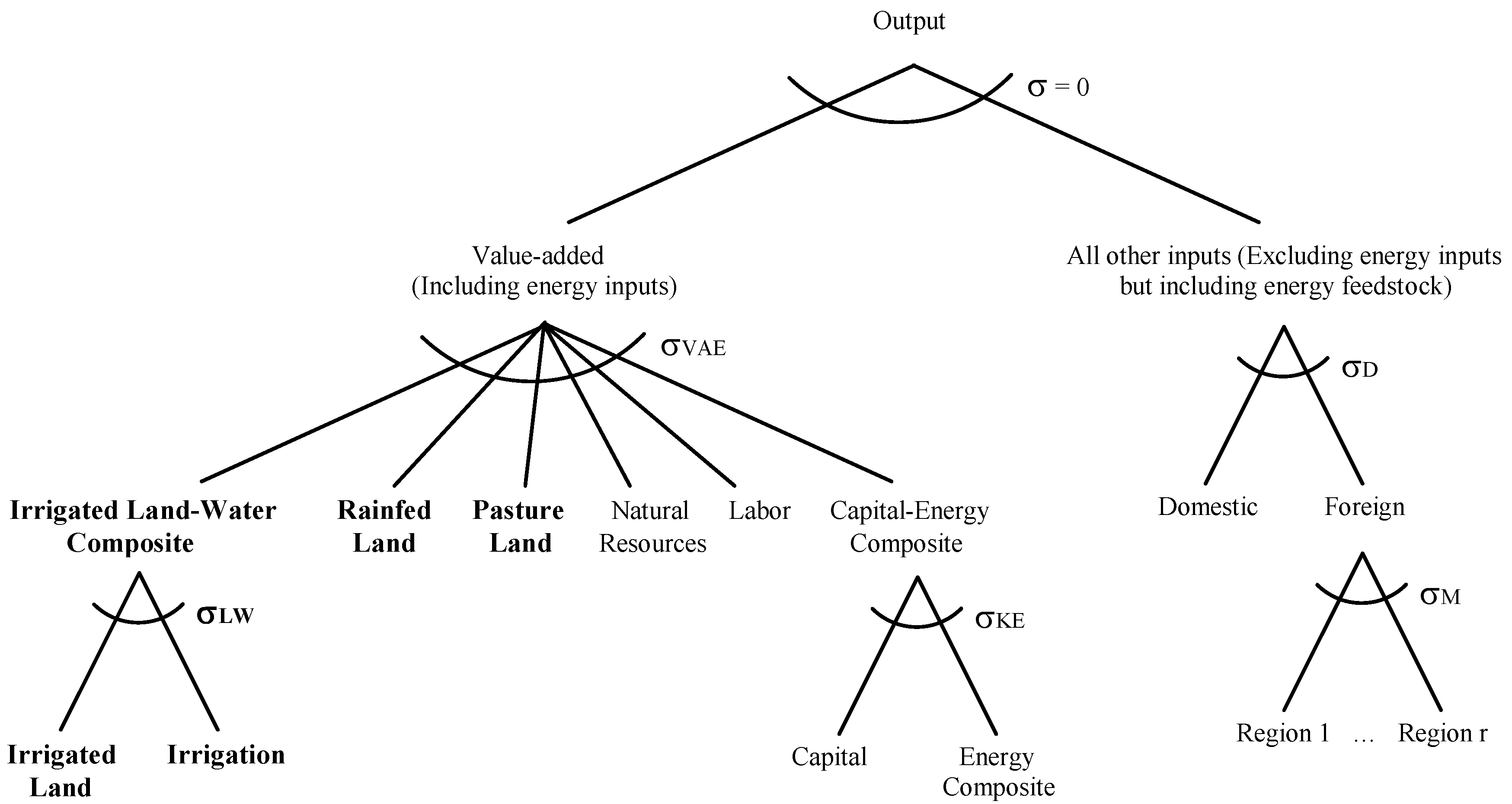
Figure A1. Nested tree structure for industrial production process in GTAP-W (truncated).
Water 03 00526 g008
Note: The original land endowment has been split into pasture land, rainfed land, irrigated land and irrigation (bold letters). σ is the elasticity of substitution between value added and intermediate inputs, σVAE is the elasticity of substitution between primary factors, σLW is the elasticity of substitution between irrigated land and irrigation, σKE is the elasticity of substitution between capital and the energy composite, σD is the elasticity of substitution between domestic and imported inputs and σM is the elasticity of substitution between imported inputs. Note that elasticities are commodity specific.
Table A1. Aggregations in GTAP-W.
A. Regional Aggregation B. Sectoral Aggregation
1. USA — United States 1. Rice — Rice
2. CAN — Canada 2. Wheat — Wheat
3. WEU — Western Europe 3. CerCrops — Cereal grains (maize, millet,
4. JPK — Japan and South Korea sorghum and other grains)
5. ANZ — Australia and New Zealand4. VegFruits — Vegetable, fruits, nuts
6. EEU — Eastern Europe5. OilSeeds —- Oil seeds
7. FSU — Former Soviet Union 6. Sug_Can — Sugar cane, sugar beet
8. MDE — Middle East 7. Oth_Agr — Other agricultural products
9. CAM — Central America 8. Animals — Animals
10. SAM — South America 9. Meat — Meat
11. SAS — South Asia 10. Food_Prod — Food products
12. SEA — Southeast Asia 11. Forestry — Forestry
13. CHI — China 12. Fishing — Fishing
14. NAF — North Africa 13. Coal — Coal
15. SSA — Sub-Saharan Africa 14. Oil —- Oil
16. ROW — Rest of the World 15. Gas — Gas
16. Oil_Pcts — Oil products
C. Endowments 17. Electricity — Electricity
Wtr — Irrigation 18. Water — Water
Lnd — Irrigated land 19. En_Int_Ind — Energy intensive industries
RfLand -— Rainfed land 20. Oth_Ind — Other industry and services
PsLand -— Pasture land 21. Mserv — Market services
Lab — Labour 22. NMServ — Non-market services
Capital — Capital
NatlRes — Natural resources

Annex B

Table B1. 2000 baseline data: Crop harvested area and production by region and crop.
Rainfed AgricultureIrrigated AgricultureTotalShare of irrigated
DescriptionAreaProductionAreaProductionAreaProductionagriculture in total:
(thousand ha)(thousand mt)(thousand ha)(thousand mt)(thousand ha)(thousand mt)Area (%)Production (%)
Regions
United States35,391209,83367,112440,470102,503650,30365.567.7
Canada27,26765,2537176,06527,98471,3182.68.5
Western Europe59,494462,34110,130146,76869,624609,10814.524.1
Japan and South Korea1,55323,0804,90971,0566,46294,13676.075.5
Australia and New Zealand21,19667,2042,23727,35323,43394,5579.528.9
Eastern Europe37,977187,4685,95840,47043,935227,93913.617.8
Former Soviet Union85,794235,09516,79374,762102,587309,85716.424.1
Middle East29,839135,15121,450118,98951,289254,14041.846.8
Central America12,970111,6158,74589,63721,715201,25240.344.5
South America79,244649,4199,897184,30489,141833,72311.122.1
South Asia137,533491,527114,425560,349251,9581,051,87745.453.3
Southeast Asia69,135331,69827,336191,84696,471523,54328.336.6
China64,236615,196123,018907,302187,2541,522,49865.759.6
North Africa15,58751,0567,35278,78722,938129,84332.060.7
Sub-Saharan Africa171,356439,4925,99443,283177,349482,7753.49.0
Rest of the World3,81047,4661,09323,9314,90371,39722.333.5
World852,3814,122,894427,1643,005,3711,279,5457,128,26533.442.2
Crops
Rice59,678108,17993,053294,934152,730403,11360.973.2
Wheat124,147303,63890,492285,080214,639588,71842.248.4
Cereal grains225,603504,02869,402369,526295,005873,55423.542.3
Vegetables, fruits, nuts133,7561,374,12836,275537,730170,0311,911,85821.328.1
Oil seeds68,847125,48029,57873,89898,425199,37930.137.1
Sugar cane, sugar beet16,457846,1379,241664,02325,6991,510,16136.044.0
Other agricultural products223,894861,30399,122780,180323,0171,641,48330.747.5
Total852,3814,122,894427,1643,005,3711,279,5457,128,26533.442.2
Note: 2000 data are three year average for 1999-2001.Source: IMPACT, 2000 baseline data (April 2008).
Table B2. No climate change simulation: Percentage change in crop harvested area and production by region and crop (2020 and 2050 relative to 2000).
Rainfed AgricultureIrrigated AgricultureTotalShare of irrigated agriculture in total
DescriptionArea (%)Production (%)Area (%)Production (%)Area (%)Production (%)Area (%)Production (%)
2020205020202050202020502020205020202050202020502020205020202050
Regions
United States−4.14−10.3427.6071.381.433.5837.6398.10−0.49−1.2334.3989.481.934.872.414.55
Canada−7.98−19.9524.5049.17−5.40−13.4923.0158.95−7.91−19.7824.3750.002.737.84−1.105.97
Western Europe−13.23−33.082.13−2.18−7.30−18.2413.3128.50−12.37−30.924.825.215.7918.358.1022.14
Japan and South Korea−11.51−28.768.6118.49−9.28−23.211.651.80−9.82−24.543.365.890.591.77−1.65−3.86
Australia and New Zealand−2.35−5.8723.9462.42−0.92−2.3029.5779.31−2.21−5.5325.5767.311.323.423.197.18
Eastern Europe−9.18−22.9412.1823.89−7.34−18.3631.7672.49−8.93−22.3215.6632.521.745.1113.9230.16
Regions
Former Soviet Union−2.57−6.4231.7375.580.270.6834.4790.91−2.10−5.2632.3979.282.426.261.576.48
Middle East1.323.2921.0256.035.1812.9548.73135.082.937.3334.0093.042.185.2311.0021.77
Central America1.403.5146.28132.717.3018.2552.26146.863.789.4548.94139.013.398.042.233.28
South America10.5126.2777.50243.3914.7736.9386.76266.2710.9827.4579.55248.453.427.444.025.11
South Asia−11.65−29.1312.2631.2310.5326.3146.70129.70−1.58−3.9530.6183.6912.3031.5112.3225.05
Southeast Asia4.7311.8329.9681.670.451.1147.20135.433.528.7936.28101.37−2.97−7.068.0116.91
China−3.85−9.6312.4231.46−1.77−4.4311.7930.47−2.49−6.2112.0430.870.731.90−0.23−0.31
North Africa2.726.8043.74122.975.0912.7335.77101.933.488.7038.91110.201.563.71−2.26−3.94
Sub−Saharan Africa13.4233.5451.39143.6530.9377.3297.97303.8114.0135.0255.56158.0114.8431.3327.2656.51
Rest of the World6.5616.4151.15146.8912.2230.5575.96226.207.8319.5659.46173.474.079.1910.3419.28
Total−0.06−0.1631.3187.973.488.7034.8596.821.122.8032.8091.702.345.741.542.67
Crops
Rice−9.85−24.63−0.65−2.90−1.46−3.6411.1526.52−4.74−11.847.9818.623.449.302.936.65
Wheat−5.57−13.9317.9540.86−1.63−4.0731.6575.50−3.91−9.7724.5957.632.376.325.6711.33
Cereal grains−1.37−3.4228.3370.736.0315.0742.06113.460.370.9334.1488.805.6314.015.9113.06
Vegetables, fruits, nuts5.0912.7226.8070.7910.4526.1339.26109.136.2315.5830.3081.573.979.136.8715.18
Oil seeds2.887.207.8418.553.137.8227.4071.892.957.3915.0938.320.170.4110.7024.27
Sugar cane, sugar beet26.1065.2674.19230.8223.8559.6362.77188.2925.2963.2369.17212.12−1.15−2.21−3.78−7.63
Other agricultural products1.012.5310.2923.266.6616.6515.4539.342.746.8612.7430.903.819.162.406.44
Total−0.06−0.1631.3187.973.488.7034.8596.821.122.8032.8091.702.345.741.542.67
Note: 2020 values are obtained by linear interpolation between 2000 baseline data and 2050 simulation without climate change.
Table B3. Change in agricultural production in 2020 and 2050 (in %) relative to baseline.
DescriptionTL1TL2A1BA2A1B + TL1A1B + TL2A2 + TL1A2 + TL2
2020205020202050202020502020205020202050202020502020205020202050
Regions
United States −0.97−0.41−0.75−0.35−1.61−9.20−3.73−10.12−2.39−9.40−2.20−9.36−4.31−10.31−4.15−10.28
Canada 2.190.664.251.76−2.02−10.04−0.05−8.530.14−9.532.08−8.782.13−7.994.11−7.21
Western Europe −1.260.21−2.21−0.412.094.302.724.830.684.73−0.254.191.305.270.404.72
Japan and South Korea−1.34−0.26−2.110.221.086.471.316.86−0.296.61−1.067.52−0.067.01−0.807.85
Australia and New Zealand2.031.482.201.497.166.9510.769.498.138.408.358.4111.1810.9011.4310.93
Eastern Europe −0.24−0.14−0.49−0.241.412.591.382.291.112.490.862.431.082.180.832.12
Former Soviet Union−0.20−0.15−0.23−0.18−4.19−21.28−4.95−20.42−4.05−21.30−4.10−21.28−4.77−20.41−4.82−20.39
Middle East 0.750.110.680.08−1.83−23.24−3.62−16.81−1.12−23.23−1.18−23.22−2.91−16.76−2.97−16.75
Central America −0.08−0.12−0.02−0.190.42−1.70−0.75−2.700.33−1.810.38−1.89−0.83−2.80−0.80−2.88
South America 0.720.210.950.16−0.12−1.770.19−1.810.54−1.650.73−1.760.83−1.701.03−1.80
South Asia −0.61−0.73−0.72−0.76−1.87−3.16−0.92−2.17−2.39−3.89−2.50−3.84−1.49−2.97−1.59−2.93
Southeast Asia 0.100.010.120.04−5.48−11.63−6.41−12.28−5.38−11.74−5.35−11.68−6.31−12.40−6.28−12.34
China 0.460.200.590.371.8611.181.779.042.2711.542.4711.882.169.362.369.68
North Africa −0.070.12−0.68−0.17−0.29−8.90−0.42−13.73−0.41−8.91−0.98−9.00−0.54−13.73−1.10−13.81
Sub−Saharan Africa0.20−0.290.25−0.390.793.541.293.690.953.241.023.131.443.391.523.28
Rest of the World1.110.911.100.93−1.41−3.58−1.09−3.64−0.41−2.82−0.42−2.79−0.07−2.89−0.08−2.86
Total0.01−0.060.01−0.08−0.45−2.28−0.53−2.38−0.44−2.31−0.44−2.29−0.53−2.43−0.52−2.42
Crops
Rice−0.19−0.50−0.12−0.49−1.27−4.09−1.28−4.17−1.44−4.53−1.37−4.50−1.45−4.60−1.38−4.57
Wheat0.15−0.160.26−0.23−0.47−4.97−0.60−3.72−0.39−5.39−0.29−5.38−0.57−4.24−0.45−4.21
Cereal grains0.010.09−0.010.07−0.29−3.32−0.64−3.41−0.28−3.23−0.31−3.24−0.63−3.34−0.65−3.34
Vegetables, fruits, nuts0.080.020.100.03−0.42−1.36−0.36−1.41−0.34−1.28−0.31−1.23−0.27−1.35−0.25−1.29
Oil seeds−0.98−1.79−1.15−2.19−0.57−3.71−1.29−4.28−1.40−4.89−1.60−5.36−2.01−5.41−2.23−5.87
Sugar cane, sugar beet−0.04−0.04−0.09−0.10−0.54−3.37−0.55−3.31−0.60−3.43−0.64−3.48−0.60−3.37−0.65−3.42
Other agricultural products0.110.040.110.12−0.241.19−0.360.10−0.151.35−0.101.52−0.280.23−0.230.38
Total0.01−0.060.01−0.08−0.45−2.28−0.53−2.38−0.44−2.31−0.44−2.29−0.53−2.43−0.52−2.42
Table B4. Change in agricultural water use in 2020 and 2050 (in %) relative to baseline.
DescriptionTL1TL2A1BA2A1B + TL1A1B + TL2A2 + TL1A2 + TL2
2020205020202050202020502020205020202050202020502020205020202050
Regions
United States−2.24−1.57−1.98−1.53−2.65−11.69−5.82−12.62−4.60−12.69−4.38−12.69−7.53−13.61−7.34−13.61
Canada2.130.523.951.33−2.27−9.70−0.23−8.25−0.19−9.311.51−8.751.85−7.843.60−7.25
Western Europe−1.80−0.21−2.98−1.042.604.833.325.530.474.80−0.694.081.175.490.054.76
Japan and South Korea−3.88−1.93−7.60−3.991.356.691.767.28−2.724.56−6.422.45−2.315.11−6.053.07
Australia and New Zealand1.360.861.610.9011.7611.8616.8515.4611.3212.7311.6512.7815.4916.2315.8516.30
Eastern Europe−0.13−0.07−0.37−0.221.222.691.302.171.002.650.772.561.082.130.862.04
Former Soviet Union−0.12−0.11−0.08−0.12−6.21−23.52−7.21−22.55−5.89−23.49−5.88−23.47−6.83−22.47−6.83−22.45
Middle East1.860.842.020.80−3.94−26.50−8.81−19.74−2.17−25.90−2.01−25.87−7.03−19.05−6.89−19.01
Central America−0.81−0.76−1.55−1.460.81−2.20−1.96−3.93−0.01−2.92−0.76−3.60−2.74−4.63−3.46−5.29
South America2.461.082.991.27−0.13−0.650.57−0.672.200.212.700.332.870.193.380.31
South Asia−0.35−0.53−0.33−0.47−3.26−3.46−1.88−2.49−3.51−4.07−3.48−3.93−2.20−3.19−2.17−3.06
Southeast Asia0.270.030.21−0.08−5.33−12.42−6.23−13.13−5.01−12.36−5.07−12.46−5.90−13.07−5.96−13.15
China0.330.020.29−0.052.0012.161.759.462.2712.272.2912.312.009.552.019.57
North Africa0.140.10−0.48−0.09−2.85−8.76−2.41−10.89−2.78−8.89−3.39−8.93−2.35−10.78−2.94−10.81
Sub−Saharan Africa0.460.010.45−0.050.873.261.483.601.273.231.283.151.853.571.873.50
Rest of the World0.750.560.720.59−3.03−5.09−2.55−5.78−2.35−4.61−2.39−4.59−1.88−5.30−1.92−5.29
Total0.11−0.130.13−0.16−1.27−2.19−1.33−2.31−1.15−2.31−1.13−2.31−1.22−2.45−1.20−2.45