3.1. Experimental Results
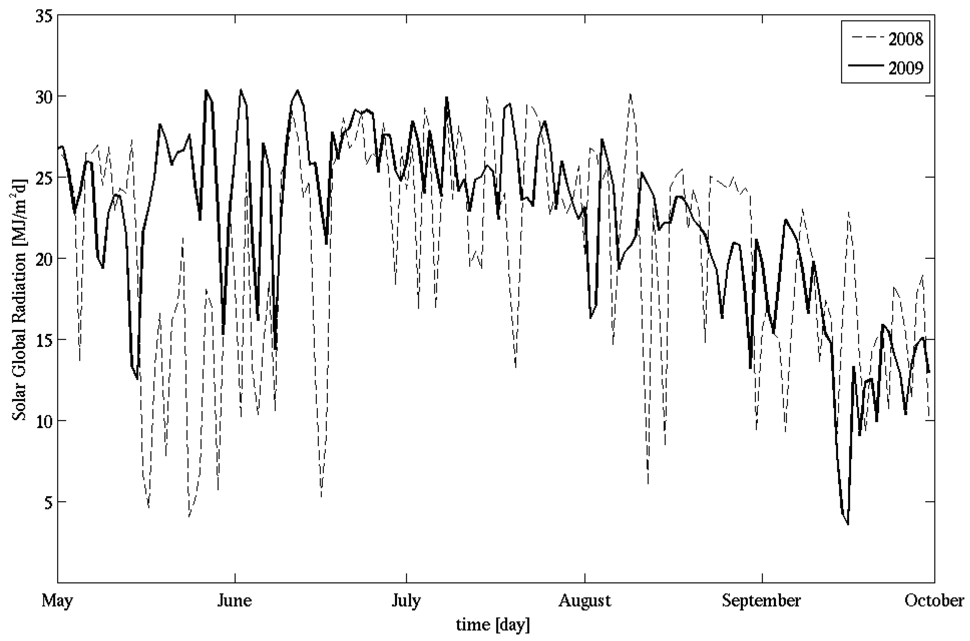
Cocconato daily values of GR ranged between 4 and 30
d
in both 2008 and 2009, with their maxima recorded during June, July and early August (during 2009), when the daily variability appeared lower. Comparing 2008 and 2009, an appreciable difference came out in the second half of May: the 2009 values were on average 15
d
higher than those of 2008 (
Figure 1).
Figure 1.
Daily values of solar global radiation (in MJ m
d
), deduced by PAR observations as mentioned in
subsection 2.3 during 2008 and 2009 vegetative seasons relative to the Barbera cultivar at Cocconato.
Figure 1.
Daily values of solar global radiation (in MJ m
d
), deduced by PAR observations as mentioned in
subsection 2.3 during 2008 and 2009 vegetative seasons relative to the Barbera cultivar at Cocconato.
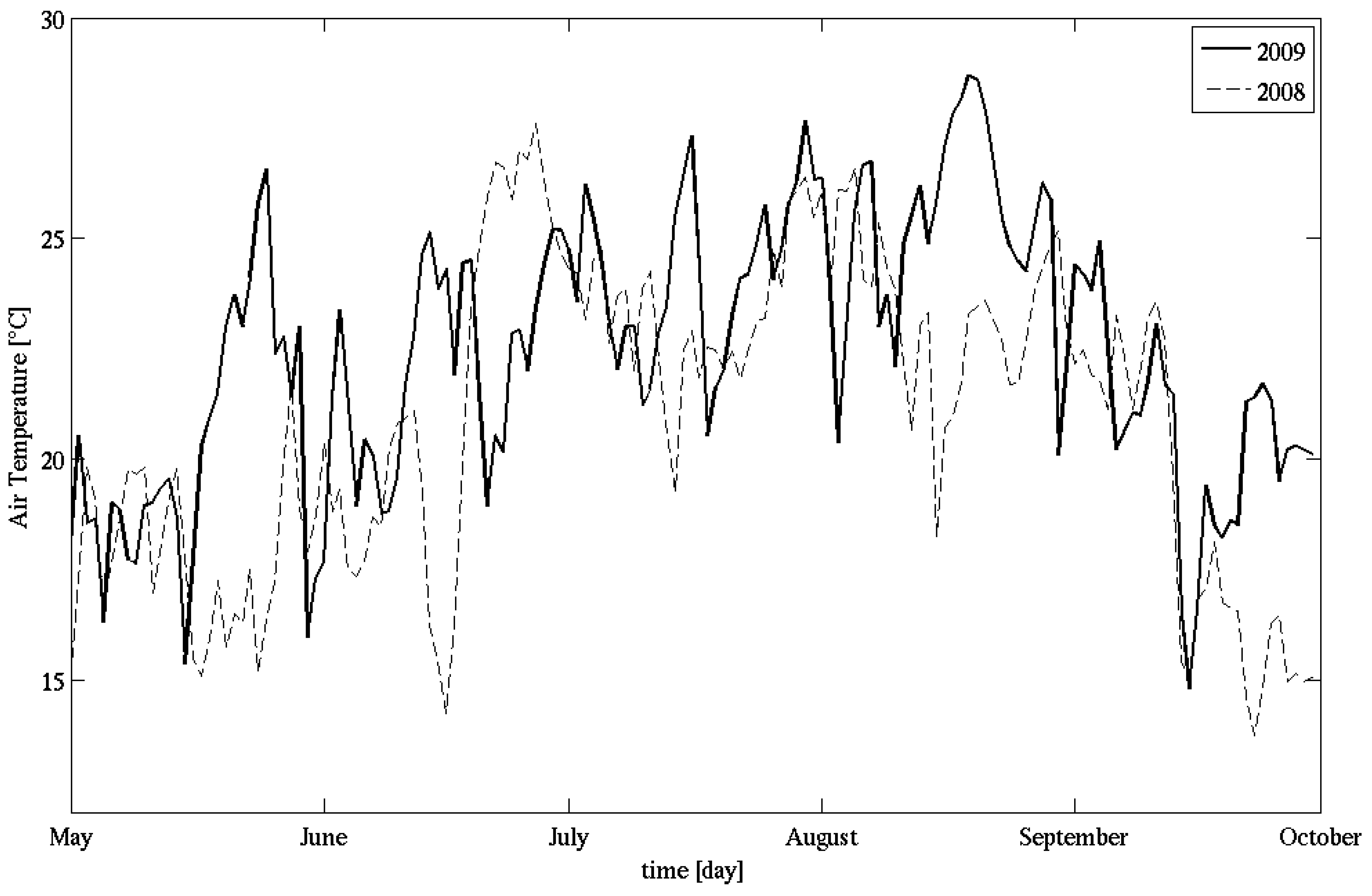
The mean daily temperature (
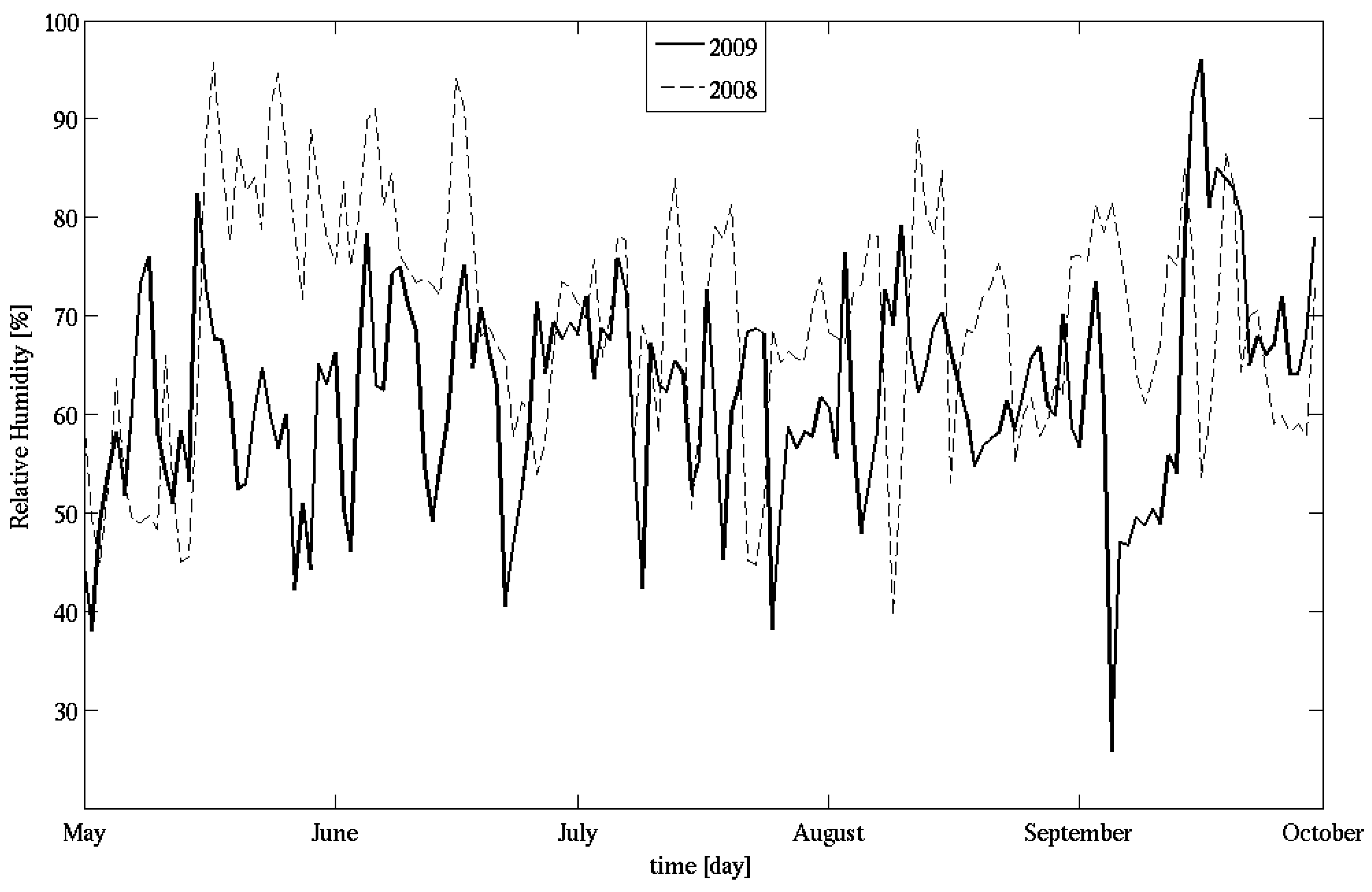
Figure 2) and humidity (
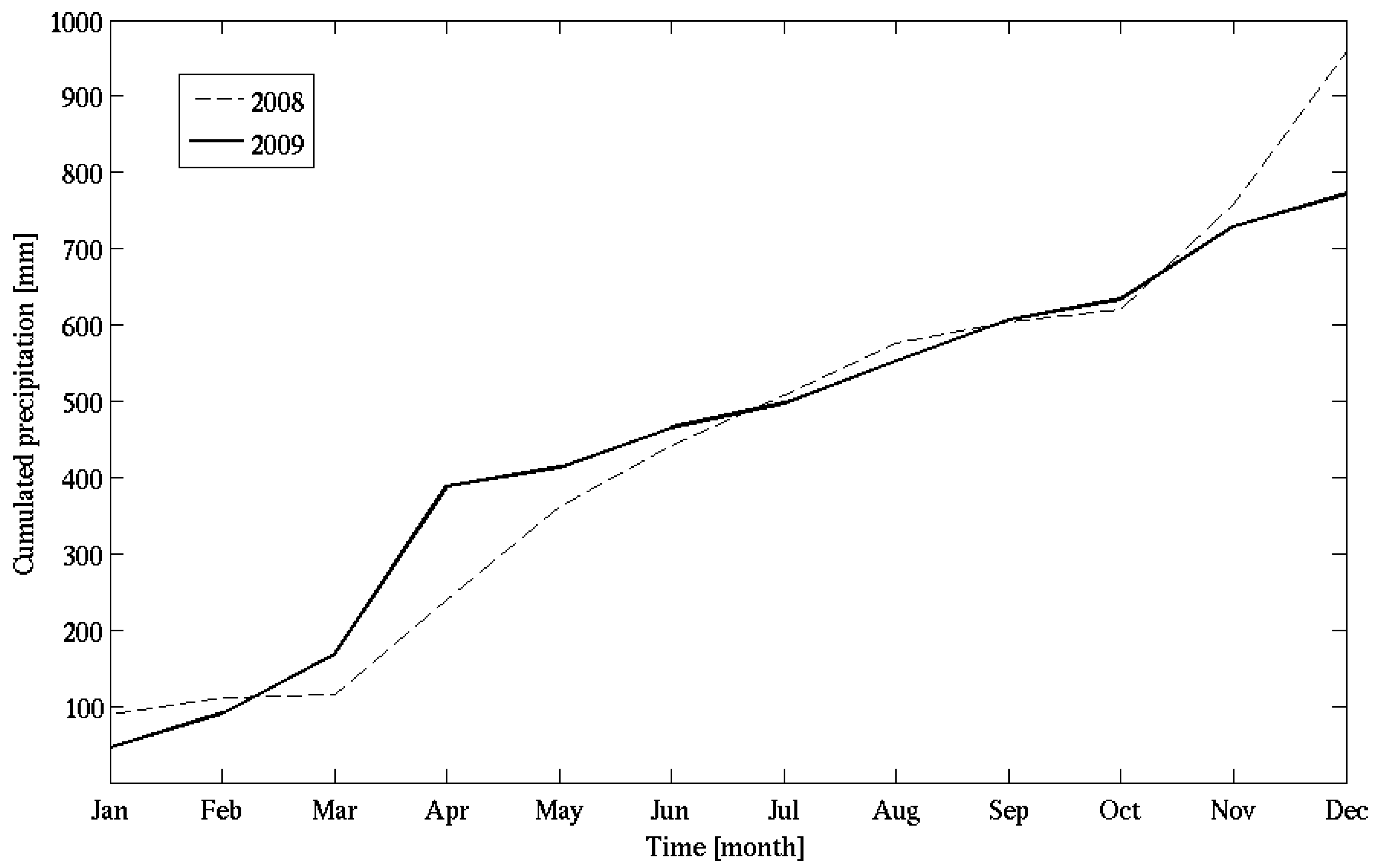
Figure 3) at screen height revealed that the 2009 vegetative season was generally warmer and drier than the 2008 one, in particular during May, August and September. This discrepancy is in part confirmed by the monthly cumulated precipitation recorded (
Figure 4), larger for 2008 (958 mm) than for 2009 (772 mm). The rainiest months were December 2008 and April 2008 and 2009, during which several episodes of intense rainfall were observed in the whole Piedmont region.
The 2009 vegetative season was analyzed with greater detail, because the number of instruments placed in the vineyard increased. The horizontal wind velocity (not shown) above the vineyard was generally low, with daily average values lower than 1 ms. More precisely, the daily averages of minimum, mean and maximum horizontal wind speeds in the period May–September, 2009, were 0.51, 0.80 and 1.64 ms, respectively (± 0.02 ms). The peak episodes tended to coincide with the passage of cyclonic areas over the site.
Figure 2.
Mean daily air temperature (in C) measured in the shelter during 2008 and 2009 vegetative seasons above the Barbera vines at Cocconato.
Figure 2.
Mean daily air temperature (in C) measured in the shelter during 2008 and 2009 vegetative seasons above the Barbera vines at Cocconato.
Figure 3.
Mean daily air relative humidity (in %) measured in the shelter during 2008 and 2009 vegetative seasons above the Barbera vines at Cocconato.
Figure 3.
Mean daily air relative humidity (in %) measured in the shelter during 2008 and 2009 vegetative seasons above the Barbera vines at Cocconato.
Figure 4.
Monthly cumulated precipitation (in mm) measured at Cocconato vineyard in 2008 and 2009.
Figure 4.
Monthly cumulated precipitation (in mm) measured at Cocconato vineyard in 2008 and 2009.
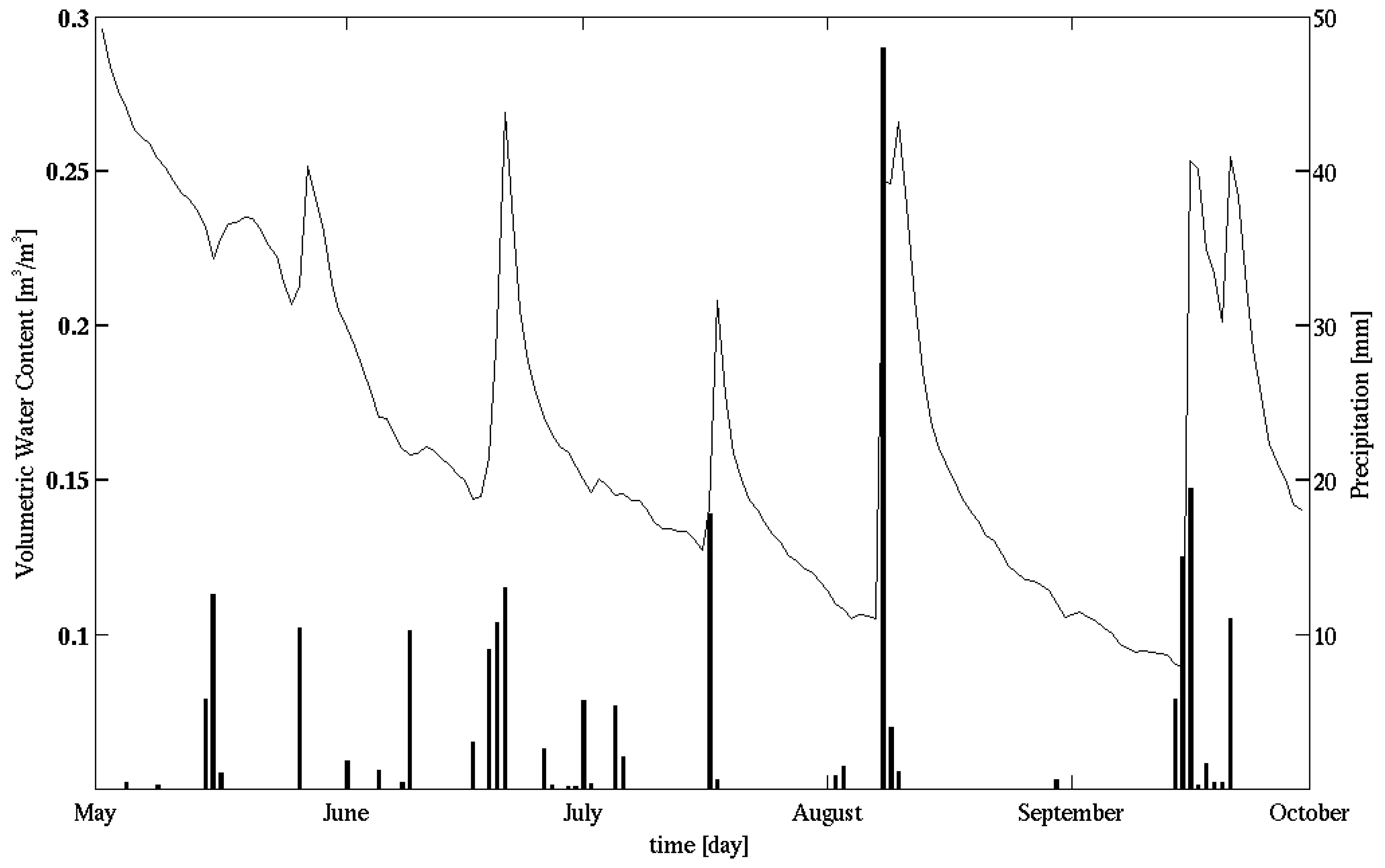
Figure 5.
Volumetric soil water content (in m
m
, left scale) measured near Barbera vine rows at Cocconato 10 cm below the soil surface, and daily cumulated precipitation (in mm, right scale) measured at Cocconato during the 2009 vegetative season. For the sake of reference, the wilting point for the silty clay loam soil is 0.22 (m
m
), while the porosity is 0.47 (m
m
) [
18].
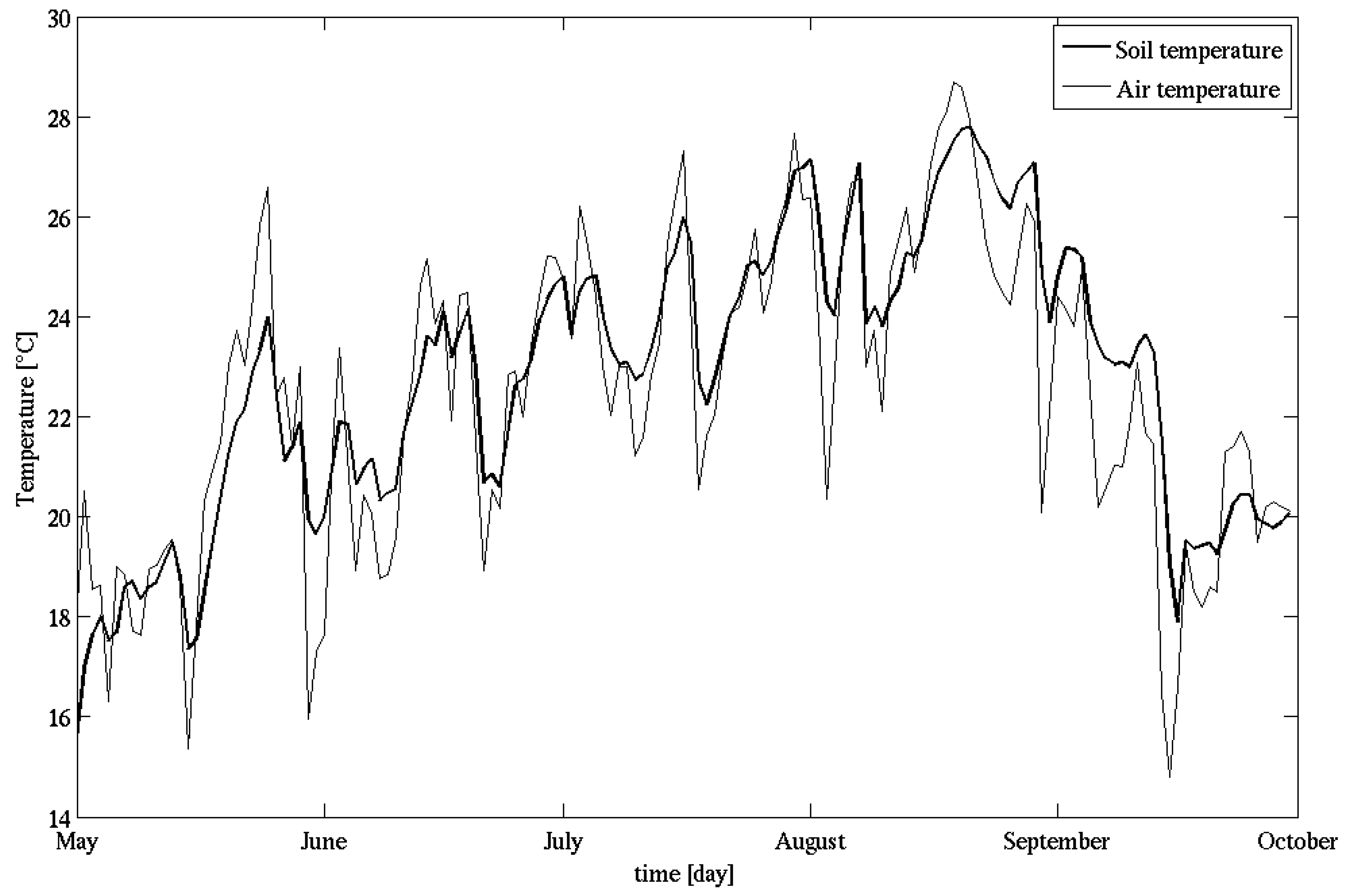
Figure 6.
Air temperature measured in the shelter, above the canopy, compared to soil temperature measured at 15 cm below the soil surface near Barbera vine rows at Cocconato, during the 2009 season at Cocconato (both in C).
Figure 6.
Air temperature measured in the shelter, above the canopy, compared to soil temperature measured at 15 cm below the soil surface near Barbera vine rows at Cocconato, during the 2009 season at Cocconato (both in C).
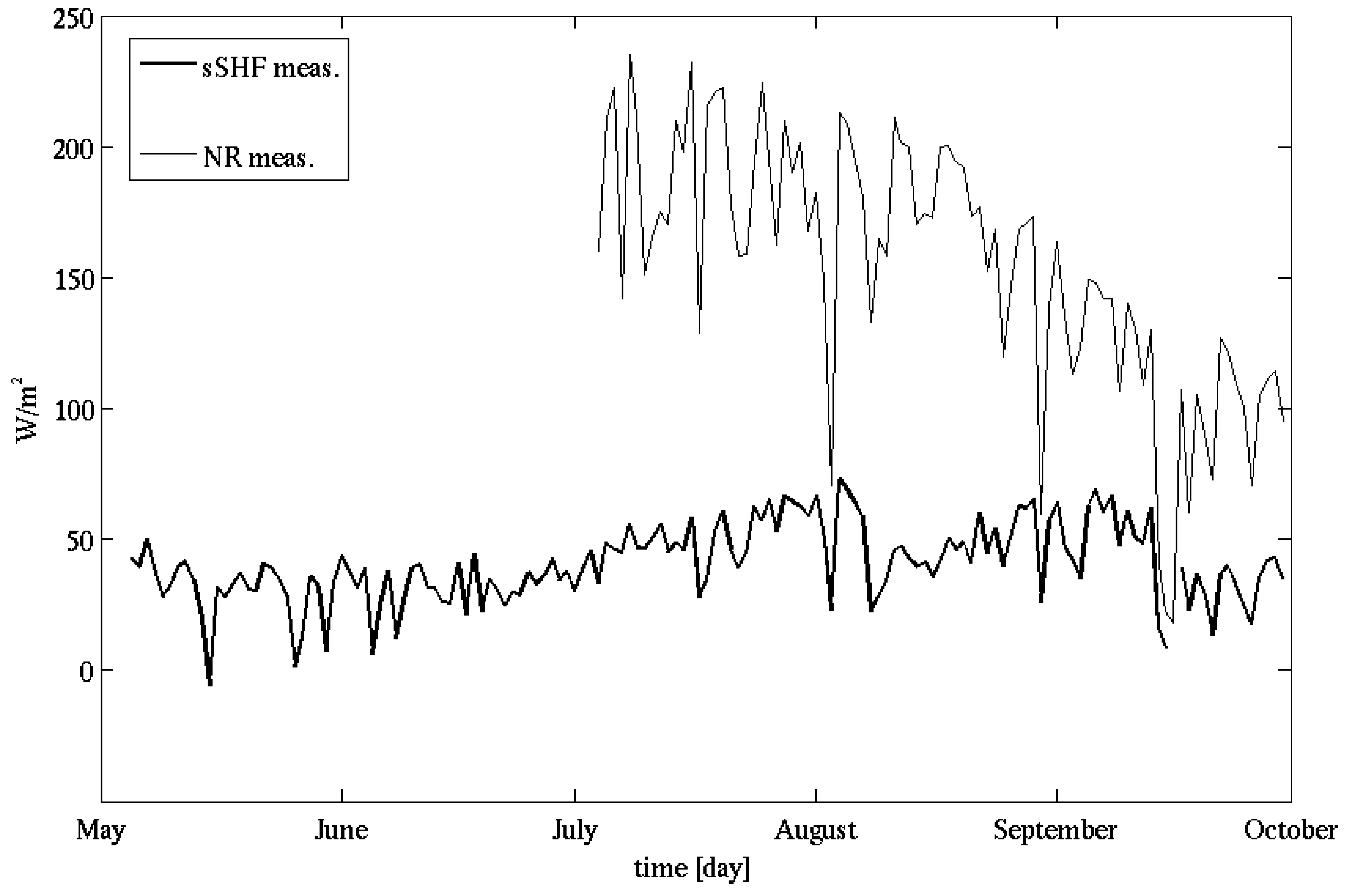
Figure 7.
Mean daily net radiation (thin line), measured at the flank of the vineyards, and “sonic” sensible heat flux (thick line), evaluated by sonic anemometer measurements above the vineyards, relative to Cocconato during the 2009 growing season (both in Wm).
Figure 7.
Mean daily net radiation (thin line), measured at the flank of the vineyards, and “sonic” sensible heat flux (thick line), evaluated by sonic anemometer measurements above the vineyards, relative to Cocconato during the 2009 growing season (both in Wm).
Figure 5 shows the measurements of the soil volumetric water content (SVWC) and the daily cumulated rainfall. The SVWC sensor was installed at 15 cm below the soil surface, but in mid July its depth was evaluated as 10 cm only, suggesting a consistent compaction of the soil above the sensor. The inspection of the data shows the rapid decrease of the SVWC, which falls below the wilting point (0.22 m
m
for this type of soil [
18]) already at the beginning of June. Apart from three large peaks in occasion of relevant rainfalls (in mid June, mid July and—the largest—at the beginning of August), SVWC reached the minimum value in mid September. The steep decrease of the SVWC, both in general and after the larger rainfall episodes (as at the beginning of August or in mid September), seems to suggest two hypothesis: i) the ET processes are important, and ii) the infiltration rate is larger than expected for the silty clay loam soil type, for which the porosity is equal to 0.47 m
m
[
18].
The soil temperature (ST), compared with air temperature measured at the screen height (
Figure 6), underlines the reduction of the amplitude in the former with respect to the latter, especially during the cold episodes (whose frequency is about two per month), usually lasting less than one week. Also a small phase shift (2–3 days) is evident during the major episodes. Both behaviors are in agreement with the theory of the thermal wave propagation into the soil [
22]. Moreover, it is possible to define the warm season using as marker the threshold of 20
C for the soil temperature (chosen for its lower daily variability, if compared with the air temperature). Neglecting the 2-days period at the end of May, it started on May 18th and ended on September 13rd.
Figure 7 shows the net radiation (NR) and the “sonic” sensible heat flux (sSHF). The former, available since the beginning of July, was characterized by a general decreasing trend, well linked with the decrease of the GR (which, in turn, depends on the solar angle and on the day duration). NR daily oscillations are in phase with those of the sSHF, and on the long trend they went closer. The sSHF was slowly increasing from mid May to the beginning of August, and then, after a drop in the first week of August, again raised until September rainfall. Daily values of the ratio beetween the measured sSHF and NR were on average 28% during July and August and 41% in the first part of September (the driest period of the 2009 vegetative season). The latter value seems in partial contrast with the data of soil moisture (
Figure 5), which showed a continuously decreasing of SVWC minima below the wilting point early June through mid September (
i.e., important ET processes).
3.2. Model Results
The two simulations, performed on a period covering both the 2008 and 2009 vegetative seasons, lasted from May 2008 until September 2009, data coinciding with the harvest time. The comparison between the two different initializations (control and experimental run) of the three vegetation parameters (LAI, vegetation cover and canopy height) is depicted in
Figure 8. The thin lines represent the data of the new vegetation class (vineyard) inserted in the Wilson and Henderson-Sellers updated database, while the thick lines are based on the observations, as explained in
subsection 2.4 The comparison among the three couple of curves in
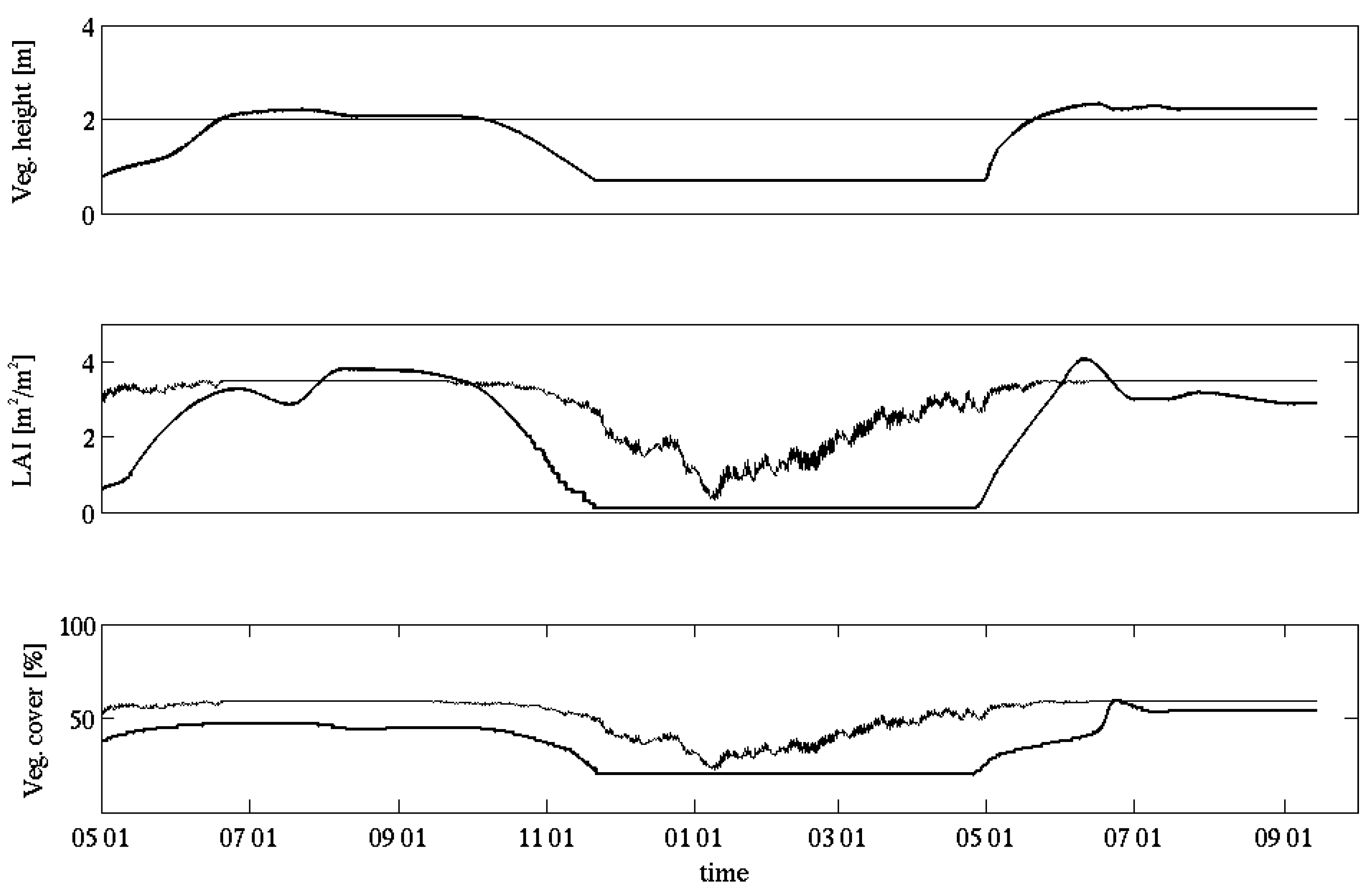
Figure 8 highlights that the experimental run parameters approach those of the control run only during the vegetative season, with an evident shift at its beginning, while during the late autumn and winter the model parameterizations underestimate consistently the observations. Moreover, the control run parameters were obviously unable to detect the lopping and thinning out of the vines, usually performed in June. Finally, the comparison between the observed time trends during 2008 and 2009 shows that the 2008 vegetative season started slightly earlier than the 2009 one, but due to the heat wave recorded in the 2009 and the contemporary cold wave recorded in the 2008 during late May (
Figure 2), the growth rate during 2009 was faster than 2008, producing an anticipation of about one week in the phenologic phase.
Figure 8.
Initialization of vegetation height, LAI and vegetation cover in the experimental run (thick line) and in the control run (thin line) from May 2008 to September 2009.
Figure 8.
Initialization of vegetation height, LAI and vegetation cover in the experimental run (thick line) and in the control run (thin line) from May 2008 to September 2009.
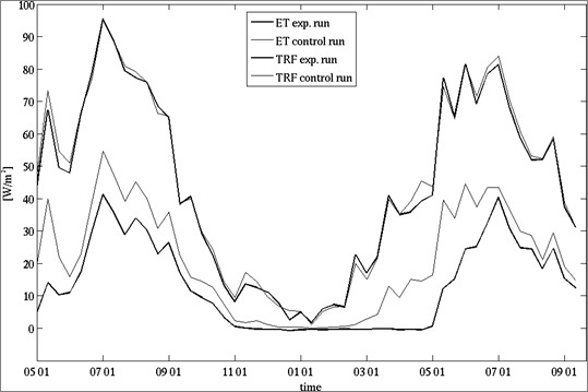
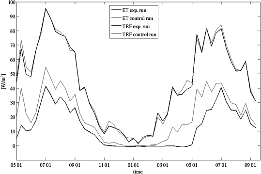
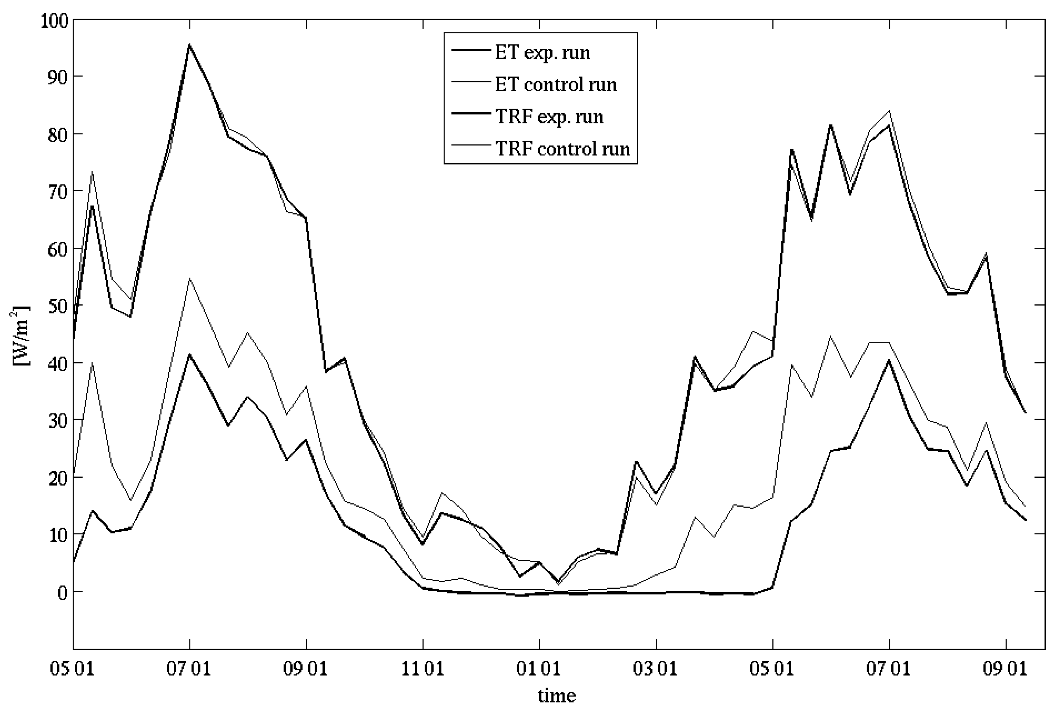
As expected from Equation 3, the discrepancy between the vegetation boundary conditions, keeping unchanged the meteorological ones, influences the transpirative part of the ET (
Figure 9) and, as a consequence, the hydrological balance. The values of the transpiration flux (hereafter TRF) in the control run are, on average, 15 Wm
higher (with peaks of 30 Wm
) than those of the experimental run during spring and summer. Comparing the two years of experimental run, the TRF during the 2009 spring is much larger than in the previous year, due to the heat wave recorded during May 2009. The behavior of TRF, as well as that of ET, is in good agreement with the observations of soil moisture, already below the wilting point on early june 2009.
The values of the latent heat flux, ET, which includes transpiration from canopy and evaporation from bare soil, are quite less sensitive to the vegetation boundary conditions, and show differences negligible in all seasons but in spring, where they reach at most 5 Wm
. The reason for such result can be arisen in the fact that the vegetation, from UTOPIA point of view, covers only partially the soil (the vegetation cover being always lower than 60%: see
Figure 8), thus the contribution of the evaporation from bare soil is relevant (about 60% for the experimental run, and about 50% for the control run), reducing the dependence of ET from the vegetation cover, LAI and canopy height.
Figure 9.
Evapotranspiration and transpiration fluxes (in Wm) evaluated by UTOPIA in the experimental run (thick line) and in the control run (thin line) from May 2008 to September 2009. Data are averaged in decades (three per month).
Figure 9.
Evapotranspiration and transpiration fluxes (in Wm) evaluated by UTOPIA in the experimental run (thick line) and in the control run (thin line) from May 2008 to September 2009. Data are averaged in decades (three per month).
The maximum ET during 2009 vegetative season is lower than that of 2008 in both simulations, with a difference of about 15 Wm during the period July–August. These results seems to suggest that there was a progressive soil drying during the 2009 summer, more intense than in the previous year and, for this reason, the available energy was progressively mostly spent for heating the surface layer (increase in SHF and decrease of ET).
The data collected with the supplementary instruments installed for the 2009 campaign allowed preliminary quantitative validations of UTOPIA in the Barbera vineyard.
The influence of the two different vegetation parameterizations on the modeled NR, SHF, ST and SVWC is quite small, and the two simulations are almost superimposed, as shown in
Figure 10 up to
Figure 13 and from the accuracy indices in
Table 2.
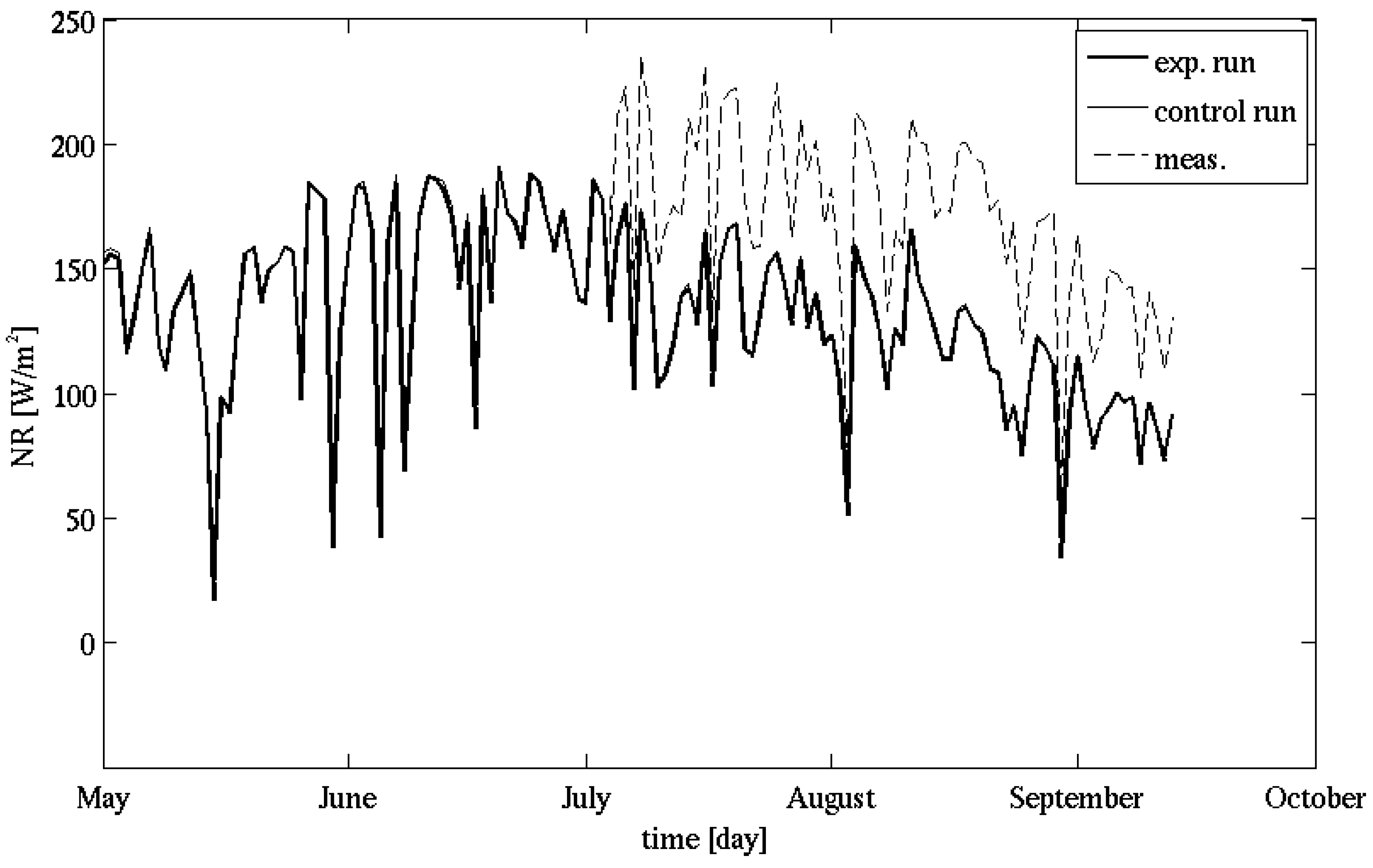
The observed NR was underestimated by about 50 Wm
in both simulations during the warmest months, and slightly less in September. The RRMSE values, equal to 30% on average, are in line with those proposed by Bellocchi
et al. [
23]. The underestimation of NR in this site can be considered as surprising, as it was never observed before in the simulations carried out using UTOPIA or LSPM, in any site. Two are the hypotheses currently advanced to explain this discrepancy. The first concerns the NR observation: Due to experimental technical requirements, the NR instrument was installed at the flank of the vineyards over the meadow,
i.e., in a different place with respect to the other sensors (installed within and above the vines). The second hypothesis, supported by the satisfactory value of the coefficient of determination r
(close to the unit) is that one or more calibration coefficients associated to vegetation or bare soil (namely, the albedo) were not accurately parameterized or the effects of the grass underlying the vines were not adequately taken into account.
Figure 10.
Mean daily values of net radiation (in Wm) during the 2009 vegetative season. The dashed line shows the measurements carried out on the flank of the vineyards, while the thick line refers to the experimental run and the thin line to the control run.
Figure 10.
Mean daily values of net radiation (in Wm) during the 2009 vegetative season. The dashed line shows the measurements carried out on the flank of the vineyards, while the thick line refers to the experimental run and the thin line to the control run.
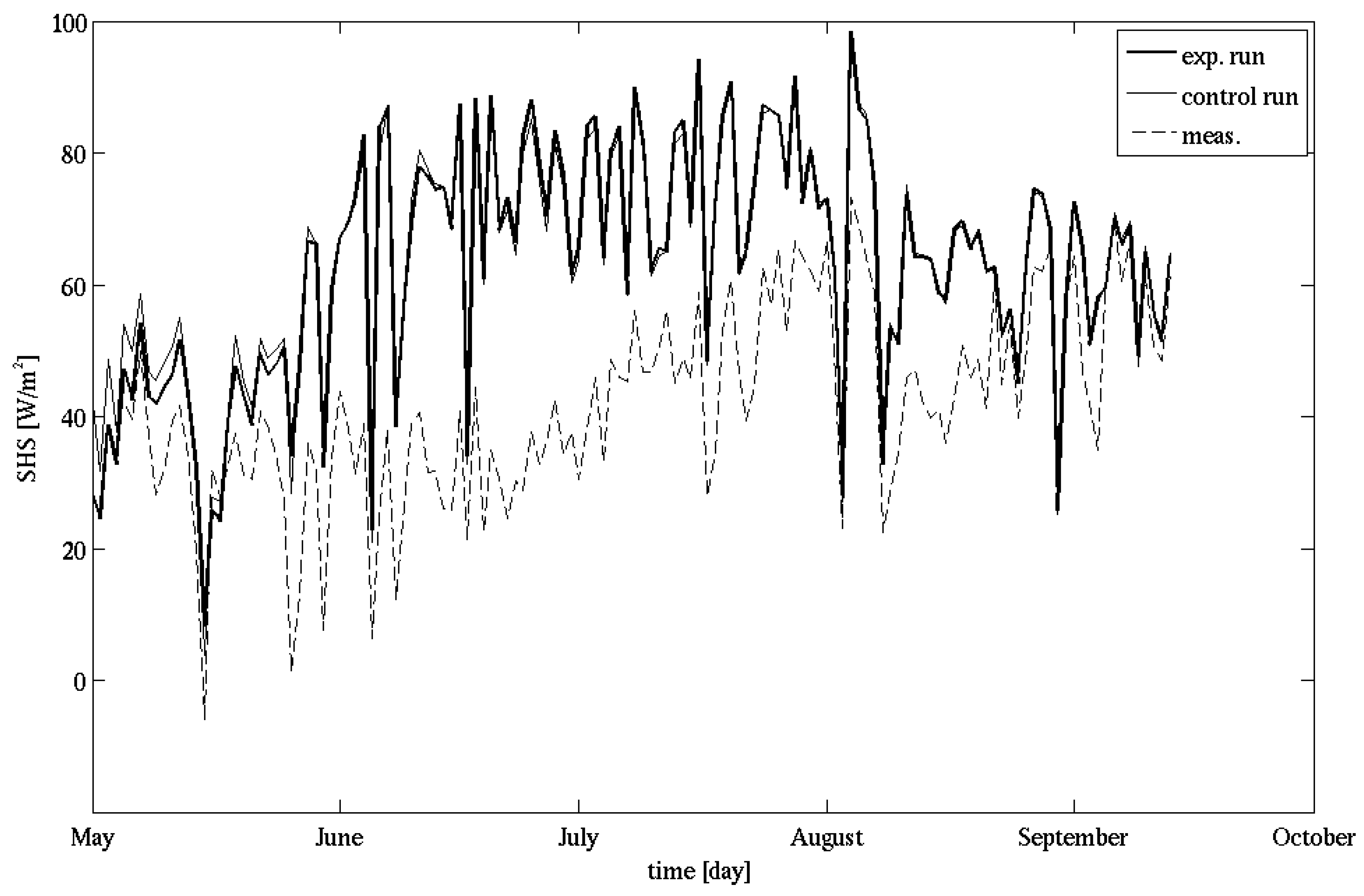
Figure 11.
Mean daily values of sensible heat flux (in Wm) during the 2009 vegetative season. The dashed line shows the values derived from the measurements carried out with the sonic anemometer above the vineyards, the thick line refers to the experimental and the thin line to the control run.
Figure 11.
Mean daily values of sensible heat flux (in Wm) during the 2009 vegetative season. The dashed line shows the values derived from the measurements carried out with the sonic anemometer above the vineyards, the thick line refers to the experimental and the thin line to the control run.
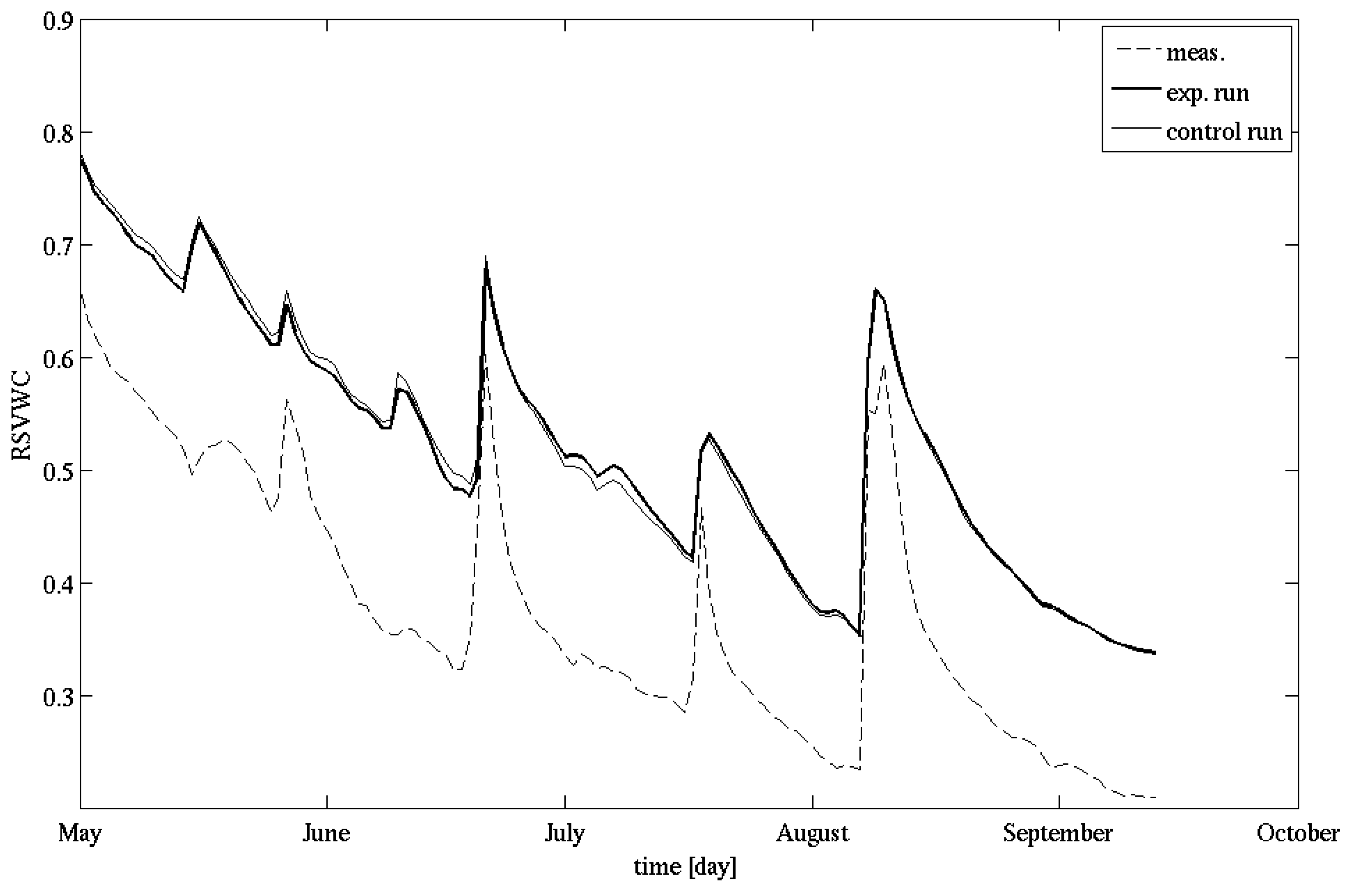
Figure 12.
Mean daily values of soil relative humidity (i.e., the volumetric soil water content normalized by the soil porosity) at 10 cm below the surface, during the 2009 vegetative season. The dashed line shows the measurements while the thick line refers to the experimental run and the thin line to the control run.
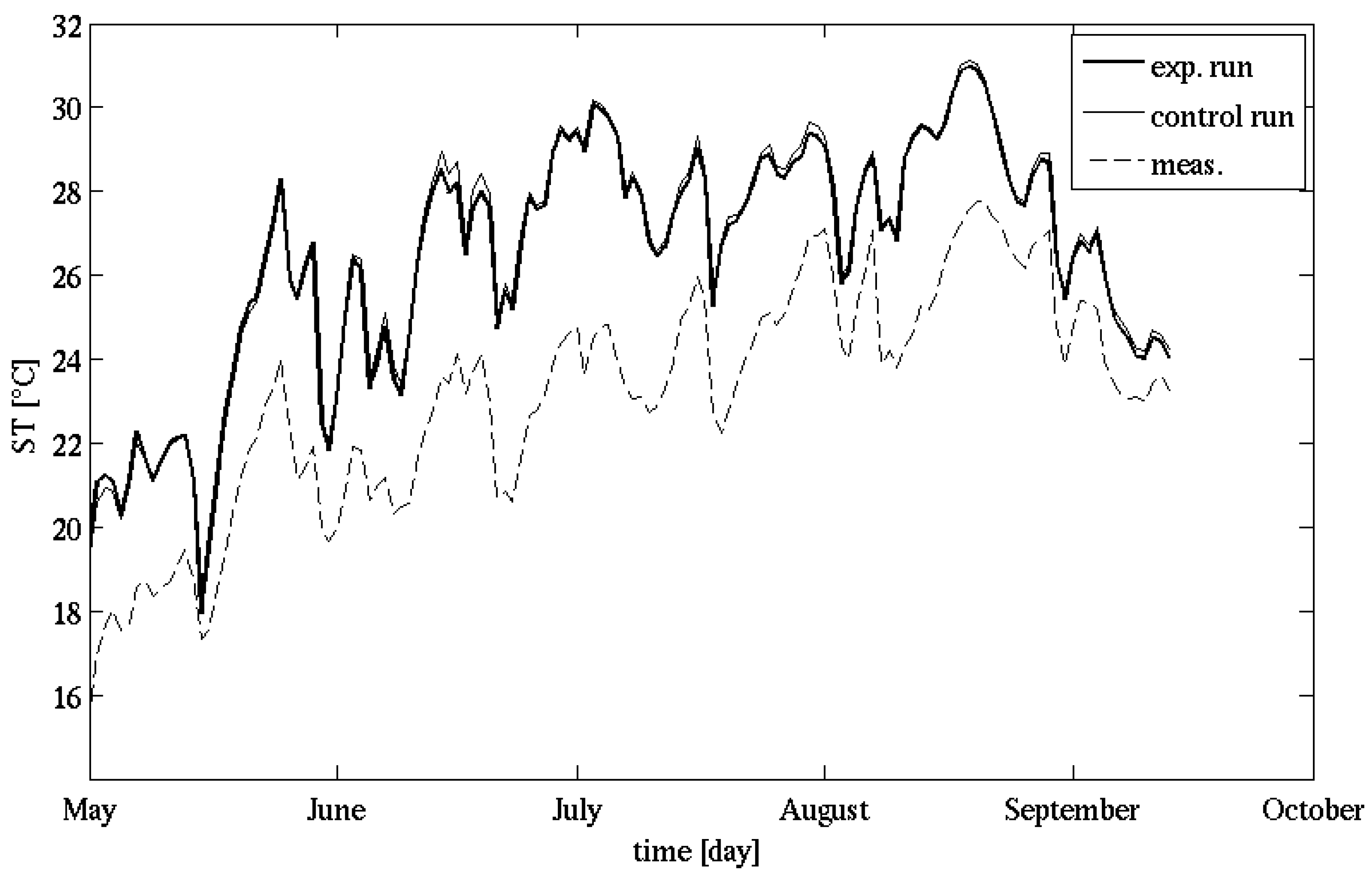
Figure 13.
Mean daily value of soil temperature at 10 cm below the surface (in C) during the 2009 vegetative season. The dashed line shows the measurements while the thick line refers to the experimental run and the thin line to the control run.
Figure 13.
Mean daily value of soil temperature at 10 cm below the surface (in C) during the 2009 vegetative season. The dashed line shows the measurements while the thick line refers to the experimental run and the thin line to the control run.
Table 2.
Indices of agreement between measured and simulated daily values of NR, SHF, RVSWC and ST from the control and the experimental runs. For NR less data are available due to the late instrument installation.
Table 2.
Indices of agreement between measured and simulated daily values of NR, SHF, RVSWC and ST from the control and the experimental runs. For NR less data are available due to the late instrument installation.
| | RRMSE (%) | r | total number of data |
| NR (control run) | 30.20 | 0.90 | 72 |
| NR (experimental run) | 30.71 | 0.90 | 72 |
| SHF (control run) | 62.43 | 0.39 | 132 |
| SHF (experimental run) | 63.27 | 0.35 | 132 |
| RVSWC (control run) | 42.42 | 0.93 | 132 |
| RVSWC (experimental run) | 39.83 | 0.93 | 132 |
| ST (control run) | 15.56 | 0.83 | 132 |
| ST (experimental run) | 15.10 | 0.82 | 132 |
Also in the case of the modeled SHF, both simulations overestimate sSHF (see
Figure 11) during the 2009 vegetative season, except in the beginning and end of the simulation (see in
Table 2 the RRMSE). The difference is about 40 Wm
at the end of June and cannot be attributed to the difference between sSHF and SHF, quantifiable in this case in few Wm
. Besides the numerical values of the fluxes, also their trend is different, as showed by the low values of the r
coefficients. UTOPIA SHF show a jump of about 30 Wm
at the end of May, then its value remains almost constant until August, with some daily fluctuations. On the contrary, the measured sSHF reveals an almost regular growth during June and early July. RRMSE values attest the graphical analysis, though being lower than other found in model accuracy literature [
24].
The differences between model and observations, for both NR and SHF variables, are reduced during rainy days (see
Figure 1 and
Figure 5).
When SHF underestimates sSHF, the ET is growing quickly (
Figure 9), thus it may be not inconsistent to hypothesize that the variation of ET may affects sSHF but not SHF. Excepting for the hottest period, in May, August and September the differences among sSHF and SHF are small and can be considered of the same order of magnitude of the error associated with the measurements (quantifiable in 10–15 Wm
).
To compare the SVWC predicted by UTOPIA with the observed data (
Figure 12), the measured SVWC was normalized with the soil porosity (equal to 0.47 m
m
for the silty clay loam soil) achieving the relative soil volumetric water content (RSVWC). The simulated values systematically overestimate the observations by 0.15–0.20 m
m
in absence of precipitation, while during and immediately after the precipitation events the overestimation is reduced to less than 0.1 m
m
. The overestimation regards both control and experimental run, whose values differ between each other for less than 10% during late spring and almost coincide later. This behavior indicates that the overestimation is not caused by the uncorrect value of the vegetation parameters, thus it may be possible to conclude that the soil type below the upper 30 cm (not measured) had a different texture. In
Figure 13 simulated and observed STs are shown. Even in this case, UTOPIA simulations overestimate almost systematically the observations, with differences slightly lower than 2
C, irrespectively of rainy or dry weather. The reason for such discrepancy may arise from the too low vegetation cover values parameterized by UTOPIA simulations (see
Figure 8).
For both ST and RSVCWC, despite the UTOPIA overestimations, emphasized by the RRMSE, the respective trends are well reproduced, as confirmed by the high values of the coefficient of determination (
Table 2).


 ,
, 
