Regionalization of SWAT Model Parameters for Use in Ungauged Watersheds

Abstract

There has been a steady shift towards modeling and model-based approaches as primary methods of assessing watershed response to hydrologic inputs and land management, and of quantifying watershed-wide best management practice (BMP) effectiveness. Watershed models often require some degree of calibration and validation to achieve adequate watershed and therefore BMP representation. This is, however, only possible for gauged watersheds. There are many watersheds for which there are very little or no monitoring data available, thus the question as to whether it would be possible to extend and/or generalize model parameters obtained through calibration of gauged watersheds to ungauged watersheds within the same region. This study explored the possibility of developing regionalized model parameter sets for use in ungauged watersheds. The study evaluated two regionalization methods: global averaging, and regression-based parameters, on the SWAT model using data from priority watersheds in Arkansas. Resulting parameters were tested and model performance determined on three gauged watersheds. Nash-Sutcliffe efficiencies (NS) for stream flow obtained using regression-based parameters (0.53–0.83) compared well with corresponding values obtained through model calibration (0.45–0.90). Model performance obtained using global averaged parameter values was also generally acceptable (0.4 ≤ NS ≤ 0.75). Results from this study indicate that regionalized parameter sets for the SWAT model can be obtained and used for making satisfactory hydrologic response predictions in ungauged watersheds.

1. Introduction

For a number of years, there has been a steady shift towards modeling and model-based approaches as primary methods of assessing watershed response to hydrologic inputs and land management and of quantifying watershed-wide best management practice (BMP) effectiveness. A variety of models have been designed for this purpose, including: the Soil and Water Assessment Tool, SWAT [1]; the Annualized Agricultural Non-Point Source model, AnnAGNPS [2]; the Areal Nonpoint Source Watershed Environment Response Simulation model, ANSWERS [3]; and, the Hydrological Simulation Program Fortran, HSPF [4,5] among others. The use of modeling, however, necessitates a certain degree of model accuracy. This can, to a large extent, be determined through comparisons of model predictions to observed data at gauging stations within the watersheds and at the watershed outlet. Where available, watershed characterization data can be used to furnish model parameters in lieu of default values, thus presumably improving model performance. Often, however, existing models require some degree of calibration and validation to achieve adequate watershed and therefore BMP representation. This, however, is only possible for gauged watersheds. Unfortunately, there are many watersheds for which there are very little or no monitoring data available, thus the question as to whether it would be possible to extend and/or generalize model parameters obtained through calibration of gauged watersheds to ungauged watersheds within the same region.

Many researchers have suggested that the accuracy of models in making watershed response predictions in ungauged watersheds can be improved by developing regionalized parameter values [6,7,8]. In parameter regionalization, parameter values are extended and/or extrapolated using calibrated values obtained from gauged watersheds located within the same region [9]. In its simplest form, regionalization estimates the mean of all available calibrated parameter values. Termed the “global average” [10], this method gives one set of values for use in all candidate watersheds. This method, however, ignores the heterogeneity among watersheds and has been found to give unsatisfactory results [10]. Several studies, including [6,7,10,11,12,13,14] have used regression models that relate model parameters to watershed and climatic characteristics to determine regionalized parameter values. In summary, these studies have found regression to give suitable parameter estimates. However, parameter sets so developed were found to work better on lumped (as compared to distributed) models, and in models that did not have a large number of parameters [12,14]. Kriging (geostatistical methods of spatial interpolation) has also been used successfully in regionalization [10,15]. The success of kriging is, however, dependent upon the availability of spatially refined datasets. Combination (hybrid) methods, which integrate a variety of regionalization methods, are possibly the most efficient of all regionalization methods [8]. Like kriging, these methods require a large number of data (gauging) points and associated calibration parameter sets.

Although these and other related studies have had mixed results, a few methods have emerged as being commonly used methods, including: global averages [10,16]; averages based on expected similarities in watershed hydrologic responses [10,17]; bi-variate or multi-variate regression relating calibration parameters to watershed characteristics [8,16,18]; kriging [8,10]; and combination (hybrid) methods [8].

The objective of this study was to evaluate two regionalization methods (global average and regression) as tools for developing SWAT parameter values so that the model can be applied in ungauged watersheds with a certain degree of accuracy. These two methods were selected because they are among the commonly used approaches, and available data were sufficient for the required analyses. The use of kriging and hybrid methods was not explored as these would require more spatially refined model parameter datasets than were available. Watersheds used in parameter regionalization were located in Arkansas. Datasets used in this study were developed based on previous modeling work conducted at the 8-digit hydrologic unit code (HUC) level [19] in seven Arkansas’ priority watersheds [20,21,22].

Regionalized parameter values were tested on three gauged watersheds in Arkansas, one of which was independent of the seven that had been used to derive the regional parameter sets. We first present the regionalized parameter sets as obtained through each of the regionalization methods, and the associated model performance in comparison to the calibrated model. We then present an inter-comparison of the regionalization methods based on model performance obtained using parameter values determined from each of the methods. Finally, we discuss our experience with regionalization and the suitability of the various methods in obtaining model parameter sets for watershed response predictions.

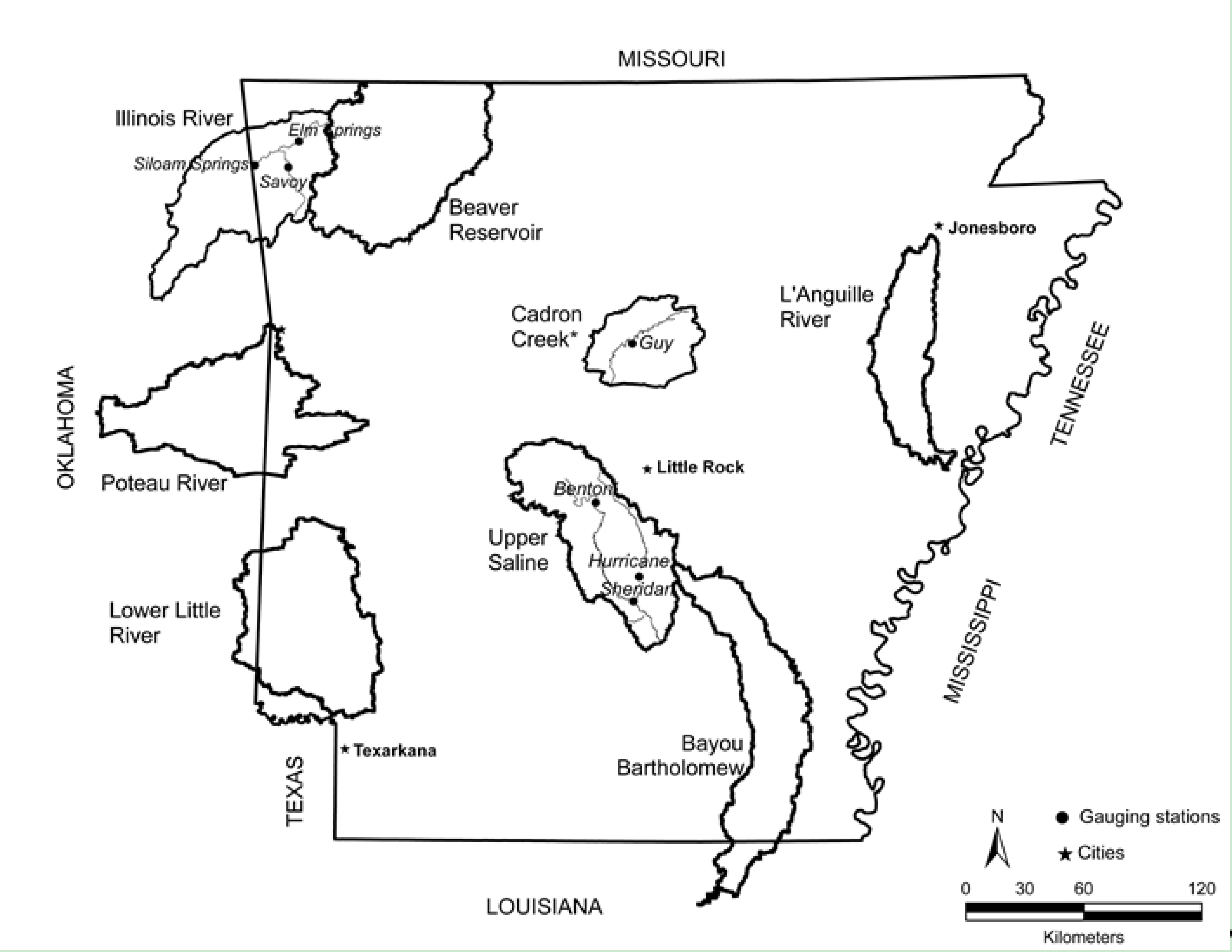
1.1. Site Description

This study used data from seven different watersheds located in Arkansas (Figure 1). These seven watersheds are designated by the Arkansas Natural Resources Commission (ANRC) as priority watersheds for nonpoint source pollution control. These watersheds include: Bayou Bartholomew, Beaver Reservoir, Illinois River, L’Anguille River, Lower Little River, Poteau River, and Upper Saline (Figure 1). They range in size from 1,400 km² (Poteau River) to 6,600 km² (Beaver Reservoir). With the exception of the L’Anguille River watershed, these watersheds are dominated by forests (56%–77%). The L’Anguille River watershed lies within the main crop production region of Arkansas and is dominated by rice/soybean rotations (71%). Slopes in most of the watersheds are predominantly in the 0-3% slope class, with the exception of Beaver Reservoir and Illinois River watersheds. The Beaver Reservoir watershed has the slope ranges 0–3%, 3–8%, 8–15%, 15–25%, and >25% distributed almost equally across the watershed, while the Illinois watershed comprises almost equal areas in the 0–3% and 8–15% slope classes. Average annual precipitation (10-yr) in these watersheds ranges between 1,100 mm and 1,400 mm while mean daily temperatures range from 14 °C (57 °F) in the northwest to 17 °C (63 °F) in the southeast. Modeling assessments have previously been carried out [20,21,22] to locate high pollutant source areas within these watersheds and, subsequently, to develop BMPs to control or reduce pollutant losses from these areas. These modeling assessments need to be extended to other watersheds experiencing similar NPS pollution problems in the State. Most of these other watersheds, however, are either ungauged or have insufficient data to support model calibration/validation.

Figure 1. Locations of watersheds and primary gauging stations used in the study (Gauging station locations are only shown for test watersheds).

Figure 1. Locations of watersheds and primary gauging stations used in the study (Gauging station locations are only shown for test watersheds).

*Cadron Creek watershed was not used in deriving regionalized parameters. However, it was used as an external watershed in testing parameter performance following regionalization. Other watersheds used in testing the suitability of regionalized parameters were Illinois River (Arkansas portion) and Upper Saline River watersheds.

1.2. Soil and Water Assessment Tool (SWAT) Model Description

The SWAT model is a continuous simulation, daily time step, distributed parameter, watershed model developed to simulate effects of various land management and climatic scenarios on hydrologic and water quality response of agricultural watersheds [1]. The model divides watersheds into subwatersheds and further into hydrologic response units (HRUs) based on land use, soil, and slope (for ArcSWAT) information. All model outputs can be evaluated at heterogeneous spatial scales ranging from HRUs to watersheds. The SWAT model has been applied extensively in the US and many other countries to make watershed management decisions [21,23,24,25] and has also been coupled successfully with other modeling applications, for example, in-stream and riparian models, as well as geospatial and optimization tools [26,27,28,29]. The model requires several parameters (specified at the watershed, sub-basin, and HRU levels) to simulate hydrologic and water quality processes. These include weather, soils, ground water, channel, plant water use, plant growth, soil chemistry, and water quality parameters, as well as sub-basin and HRU characterization data. The SWAT model contains built-in climate, soils, and plant growth databases that can be used as data sources for climate, soil, and plant growth parameters. The basic parameters, however, are those pertaining to land use, soil, topography and climate. The model sets default values for the other parameters; entering known or measured values of these parameters, however, helps improve watershed representation, and possibly the overall model accuracy. The SWAT model uses runoff curve numbers or the Green-Ampt infiltration equation to estimate runoff based on the temporal resolution of input rainfall data. Curve numbers are recalculated daily, based on soil water content on that day [30]. Peak runoff rate predictions are based on a modification of the Rational Formula [31].

2. Materials and Methods

Two regionalization methods (global averages and regression) were evaluated in terms of their abilities to improve SWAT predictions in ungauged watersheds in Arkansas. Analyses were conducted using parameters developed in previous modeling work (Table 1) undertaken in seven Arkansas’ priority watersheds [20,21,22]. Table 1 shows these model parameters as used in the regionalization process. For the most part, specific values are given for the parameters. However, some parameters such as the curve number can take on a variety of values and, as such, will differ among HRUs. During calibrations, these HRU-level parameters may be changed by increasing or reducing them by a certain percentage until the calibration objective function is met. Values of these parameters have, thus, been reported as a percentage change from a specified value.

While for the most part parameter values were similar in proportion when compared among watersheds, the effective channel hydraulic conductivity (CH_K2) values obtained for the Bayou Bartholomew and Poteau River watersheds and revaporation (REVAPMN) obtained for the Upper Saline watershed seemed out of proportion in comparison to the other watersheds. The CH_K2 is a measure of the rate of water loss from the channel to ground water. Values of CH_K2 ranging between 0.025–2.5 mm/hr indicate low rates of water loss to ground water, while values greater than 127 mm/hr indicate losing streams [32]. Channels that continuously receive contributions from ground water will have a CH_K2 value of zero [30]. Both the Bayou Bartholomew and Poteau River watersheds have high CH_K2 values (149 and 141 mm/hr respectively) indicating the presence of losing streams within these watersheds. This condition (losing streams) is even more so in the Bayou Bartholomew watershed where pumping for irrigation purposes often renders aquifers dependent on streams for recharge [33]. The REVAPMN defines the threshold depth of water in the shallow aquifer for return flow to the root zone to occur, and is particularly important in areas with high water tables or those with deep-rooted crops [30]. This parameter can take on a variety of values in a watershed. For a number of the watersheds, GWQMN (threshold depth of water in the shallow aquifer required for return flow to occur) had a value of zero. This is the recommended minimum [34] as well as the default value of the parameter. Base flow will occur when the GWQMN threshold is met or exceeded; thus, zero and/or low values of the parameter can cause base flow to be overestimated.

Table 1. SWAT model parameters used in regionalization.

			Parameter value / (Percent change from default value)
Parameter description	Symbol		Bayou Bartholomew	Beaver Reservoir	Cadron Creek	Illinois River	L'Anguille River	Lower Little River	Poteau River	Upper Saline
Base flow recession factor, days	ALPHA_BF		0.368	0.600	0.028	0.737	0.048†	1.000	0.900	0.483
Ground water delay, days	GW_DELAY		41	31†	31	88	31	0.001	31	68
Ground water revaporationh coefficient	GW_REVAP		0.04	0.02†	0.30	0.05	0.08	0.07	0.02	0.10
Threshold depth for ground water flow to occur, mm	GWQMN		0†	0	3	0	0	0	0	100
Deep aquifer recharge fraction	rchrg_dp		0.10	0.05†	0.05	0.30	0.50	0.22	0.05	0.64
Threshold depth for revaporation to occur, mm	REVAPMN		1†	1	0	1	1	1	1	101
Snow fall temperature, ºC	sftmp		0.8	1.0†	1.0	1.0	0.5	3.4	1.0	0
Surface runoff lag coefficient, days	surlag		0.8	12	3	0.6	0.9	0.2	10	1
Plant uptake compensation factor	EPCO		0.7	1.0†	0.5	0.9	1.0	1.0	1.0	0.2
Soil evaporation compensation factor	ESCO		0.74	0.76	0.35	0.68	0.86	1.00	0.10	0.95†
Average slope length, m‡	SLSUBBSN		Varies†1	(−1.2%)	Varies	Varies	(6.2%)	Varies	(−25.4%)	Varies
Curve Number (AMChhII) ‡	CN2		(6.8%)	(−8.8%)	(−10.0%)	(−5.5%)	(1.8%)	(41.7%)	(10.0%)	(−26.0%)
Effective channel hydraulic conductivity, mm/hr	CH_K2		148.9	0.5†	0.03	15.0	0.5	0.5	141.0	1.7
Manning’s n	ch_n		0.014†	0.052	0.014	0.014	0.014	0.014	0.300	0.100
Soil albedo	sol_alb		0.07	0.10†	0.10	0.32	0.10	0.68	1.00	0.32
Available water capacity, m/m‡	SOL_AWC		(45.7%)	Varies†2	Varies	(43.6%)	(17.9%)	(50.0%)	(−50.0%)	(26.0%)

^hReturn flow to root zone. ^hhAntecedent moisture condition. ^†default value. ^‡Values represent percent change in parameter.¹Varies by subbasin; ²Varies by soil type and soil layer.SWAT parameter ranges (and allowable percentage changes): 0 ≥ ALPHA_BF ≥ 1; 0 ≥ GW_DELAY ≥ 500; 0.02 ≥ GW_REVAP ≥ 0.2; 0 ≥ GWQMN ≥ 5000; 0 ≥ rchrg_dp ≥ 1; 0 ≥ REVAPMN ≥ 500; −5 ≥ sftmp ≥ 5; 0.5 ≥ surlag ≥ 24; 0 ≥ EPCO ≥ 1; 0 ≥ ESCO ≥ 1; 10 ≥ SLSUBBSN ≥ 150 (−50% ≥ SLSUBBSN ≥ 50%); 35 ≥ CN2 ≥ 98 (−50% ≥ CN2 ≥ 50%); 0.01 ≥ CH_K2 ≥ 150; 0.01 ≥ ch_n ≥ 0.3; 0 ≥ sol_alb ≥ 0.25; 0 ≥ SOL_AWC ≥ 1 (−50% ≥ SOL_AWC ≥ 50%); References: [20,21,22].

Table 1. SWAT model parameters used in regionalization.

			Parameter value / (Percent change from default value)
Parameter description	Symbol		Bayou Bartholomew	Beaver Reservoir	Cadron Creek	Illinois River	L'Anguille River	Lower Little River	Poteau River	Upper Saline
Base flow recession factor, days	ALPHA_BF		0.368	0.600	0.028	0.737	0.048†	1.000	0.900	0.483
Ground water delay, days	GW_DELAY		41	31†	31	88	31	0.001	31	68
Ground water revaporationh coefficient	GW_REVAP		0.04	0.02†	0.30	0.05	0.08	0.07	0.02	0.10
Threshold depth for ground water flow to occur, mm	GWQMN		0†	0	3	0	0	0	0	100
Deep aquifer recharge fraction	rchrg_dp		0.10	0.05†	0.05	0.30	0.50	0.22	0.05	0.64
Threshold depth for revaporation to occur, mm	REVAPMN		1†	1	0	1	1	1	1	101
Snow fall temperature, ºC	sftmp		0.8	1.0†	1.0	1.0	0.5	3.4	1.0	0
Surface runoff lag coefficient, days	surlag		0.8	12	3	0.6	0.9	0.2	10	1
Plant uptake compensation factor	EPCO		0.7	1.0†	0.5	0.9	1.0	1.0	1.0	0.2
Soil evaporation compensation factor	ESCO		0.74	0.76	0.35	0.68	0.86	1.00	0.10	0.95†
Average slope length, m‡	SLSUBBSN		Varies†1	(−1.2%)	Varies	Varies	(6.2%)	Varies	(−25.4%)	Varies
Curve Number (AMChhII) ‡	CN2		(6.8%)	(−8.8%)	(−10.0%)	(−5.5%)	(1.8%)	(41.7%)	(10.0%)	(−26.0%)
Effective channel hydraulic conductivity, mm/hr	CH_K2		148.9	0.5†	0.03	15.0	0.5	0.5	141.0	1.7
Manning’s n	ch_n		0.014†	0.052	0.014	0.014	0.014	0.014	0.300	0.100
Soil albedo	sol_alb		0.07	0.10†	0.10	0.32	0.10	0.68	1.00	0.32
Available water capacity, m/m‡	SOL_AWC		(45.7%)	Varies†2	Varies	(43.6%)	(17.9%)	(50.0%)	(−50.0%)	(26.0%)

^hReturn flow to root zone. ^hhAntecedent moisture condition. ^†default value. ^‡Values represent percent change in parameter.¹Varies by subbasin; ²Varies by soil type and soil layer.SWAT parameter ranges (and allowable percentage changes): 0 ≥ ALPHA_BF ≥ 1; 0 ≥ GW_DELAY ≥ 500; 0.02 ≥ GW_REVAP ≥ 0.2; 0 ≥ GWQMN ≥ 5000; 0 ≥ rchrg_dp ≥ 1; 0 ≥ REVAPMN ≥ 500; −5 ≥ sftmp ≥ 5; 0.5 ≥ surlag ≥ 24; 0 ≥ EPCO ≥ 1; 0 ≥ ESCO ≥ 1; 10 ≥ SLSUBBSN ≥ 150 (−50% ≥ SLSUBBSN ≥ 50%); 35 ≥ CN2 ≥ 98 (−50% ≥ CN2 ≥ 50%); 0.01 ≥ CH_K2 ≥ 150; 0.01 ≥ ch_n ≥ 0.3; 0 ≥ sol_alb ≥ 0.25; 0 ≥ SOL_AWC ≥ 1 (−50% ≥ SOL_AWC ≥ 50%); References: [20,21,22].

2.1. Global Average-based Parameter Regionalization

Determination of global average parameters involved computing the mean of each of the parameters listed in Table 1, thus obtaining one value for each of the parameters. Any values exceeding the reasonable range for the parameter in question were reset to the maximum for the range. Because the intent was to find representative parameter values, where results of the regionalization yielded a value exceeding its reasonable range, it was assumed to imply that higher values of the said parameter would yield better model results, thus the decision to reset the value to the maximum for the range. These values were then written into their respective model input files for each of the test watersheds. The model was then run using the global average parameter values and the corresponding stream flow outputs were obtained.

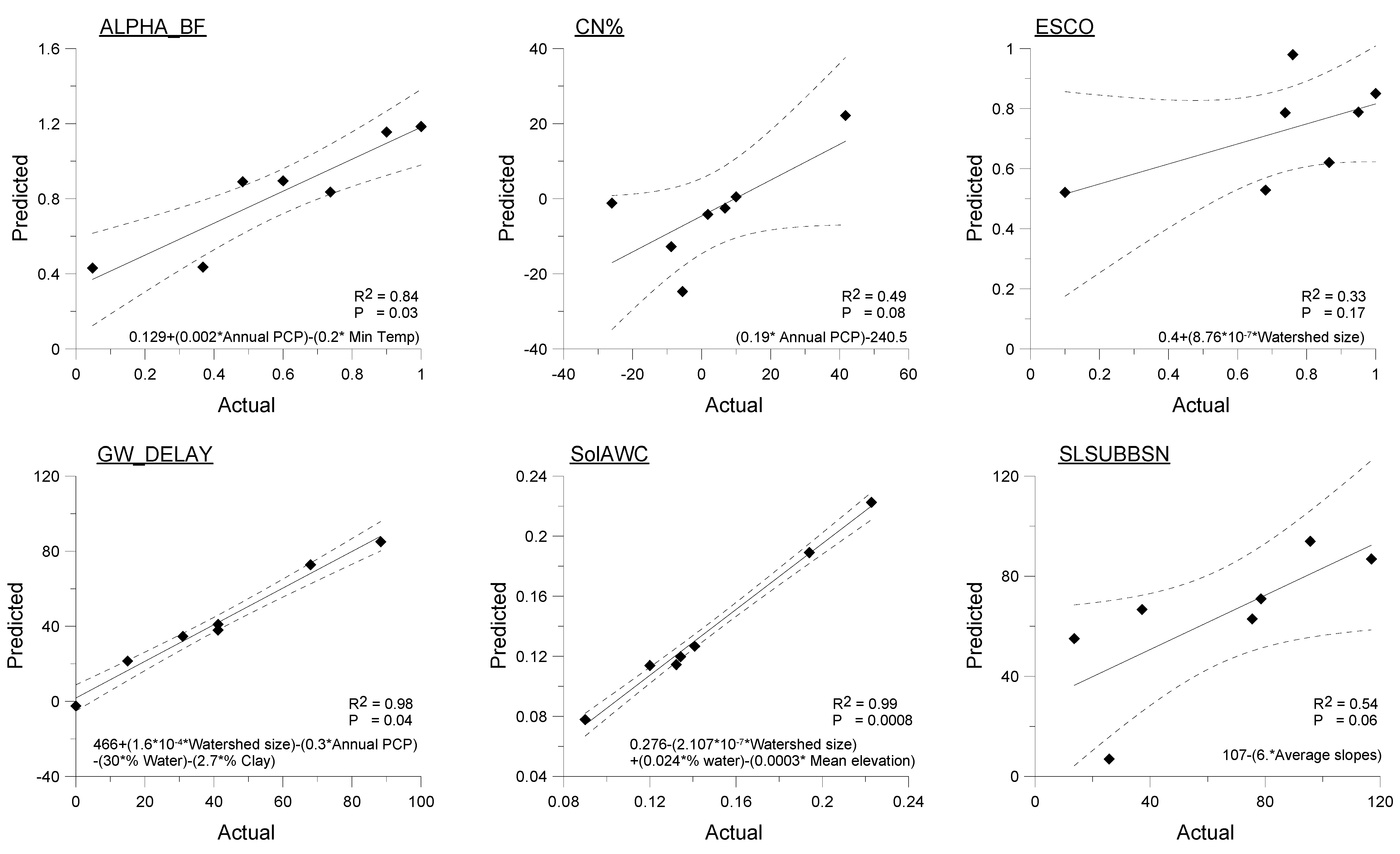
2.2. Regression-based Parameter Regionalization

A stepwise regression was used to determine functional relationships between watershed characteristics and model calibration parameters. The model performance was evaluated using regression and residual plots, r², and p- and C_p values. Where relationships obtained were significant (α = 0.1), resulting equations were used to compute model parameters for each of the test watersheds. Where no suitable equation was obtained, the corresponding global average value was used. In either case, any values exceeding the reasonable range for the parameter in question were reset to the maximum for the range. A broad range of watershed characteristics was initially defined. This was done to capture the range of topography, land use, soil, and climatic conditions that were present in the study watersheds. To avoid problems associated with collinearity between model parameters, watershed characteristics were assessed for correlation. The collinearity (r_ij²) was calculated, followed by computation of variance inflation factors (VIF = 1/(1 − r_ij²)). Collinearity was considered to exist where bivariate correlations were large (>0.8), r² of any variable(s) exceeded that of the model, and VIFs were greater than 10 [35]. If collinearity was found, only one of the characteristics concerned was included in the regression equation. Table 2 shows watershed characteristics considered in parameter regionalization. Following the regression analyses, predicted values for each of the parameters, as determined based on regression equations developed, were plotted against actual parameter values, along with their respective 95% confidence intervals. Plotting was done using Grapher^TM software.

Table 2. Watershed characteristics considered in parameter regionalization.

	Watershed
Characteristics	Bayou Bartholomew	Beaver Reservoir.	Illinois River	L’Anguille River	Lower Little River	Poteau River	Upper Saline
Size, km2	4,411	6,616	1,469	2,517	5,141	1,383	4,434
Annual precipitation, mm	1,253	1,199	1,136	1,244	1,383	1,269	1,260
Mean temperature, °C	17.2	14.1	14.0	16.4	15.0	14.2	15.2
Forest, %	56	66	37	17	67	66	77
Pastures/hay, %	3	29	55	2	28	30	20
Urban, %	2	1	8	2	1	3	2
Water, %	1.16	3.98	0.27	1.15	2.68	0.79	0.97
Clay, %	27	17	17	18	16	19	17
Silt, %	59	46	60	71	33	48	29
Mean elevation, m	73	514	439	94	392	464	307
Average slope, %	3.3	16.6	8.6	2.1	7.3	6.7	6.0

Table 2. Watershed characteristics considered in parameter regionalization.

	Watershed
Characteristics	Bayou Bartholomew	Beaver Reservoir.	Illinois River	L’Anguille River	Lower Little River	Poteau River	Upper Saline
Size, km2	4,411	6,616	1,469	2,517	5,141	1,383	4,434
Annual precipitation, mm	1,253	1,199	1,136	1,244	1,383	1,269	1,260
Mean temperature, °C	17.2	14.1	14.0	16.4	15.0	14.2	15.2
Forest, %	56	66	37	17	67	66	77
Pastures/hay, %	3	29	55	2	28	30	20
Urban, %	2	1	8	2	1	3	2
Water, %	1.16	3.98	0.27	1.15	2.68	0.79	0.97
Clay, %	27	17	17	18	16	19	17
Silt, %	59	46	60	71	33	48	29
Mean elevation, m	73	514	439	94	392	464	307
Average slope, %	3.3	16.6	8.6	2.1	7.3	6.7	6.0

2.3. Performance Analyses

Once obtained, regionalized parameters were tested on two of the priority watersheds (Upper Saline and Illinois River) and another independent watershed which was not used in regionalization analyses (Cadron Creek Watershed) (Figure 1).

Model performance was evaluated using the Nash-Sutcliffe coefficient, NS [36] the deviation from measured data, Dv [37], and stream flow hydrographs. The NS (Equation 1) is a measure of model efficiency that compares simulated values to corresponding measured values.

$$NS=1-\left(\frac{{\displaystyle \sum _{i=1}^n{(Q_i-Q_i^{\text{'}})}^2}}{{\displaystyle \sum _{i=1}^n{(Q_i-\stackrel{\_}{Q})}^2}}\right)$$

(1)

Where Q_i is the measured value (stream discharge), Q_i’ is the simulated value, $\stackrel{\_}{Q}$ is the average measured value, and n is the number of data points.

The NS can range from −∞ to 1; improved model performance is indicated as the NS approaches 1, while a value of zero indicates that simulated values are no better than the mean of observed values. While there is no consensus on specific Nash-Sutcliffe coefficient values that must be obtained for SWAT predictions to be considered good, a value greater than 0.5 is considered acceptable [38,39,40], and in particular considering monthly simulations [38,39]. Based on other documentation, NS values greater than 0.75 signify good model performance, while those between 0.36 and 0.75 signify acceptable model performance [41] (as cited in [42]). Values of NS greater than 0.4 have also been considered to indicate acceptable model performance [43]. Other criteria presented include 0.65–0.75 (fair) and 0.75–0.85 (good) with values above 0.85 representing very good model performance [44]. Within these general ranges the criteria established will often depend on the model and nature of the application, thus what is considered acceptable will vary among projects [40]. These general guidelines were used in further evaluating model performance.

The Dv is a measure of the deviation of simulated values from measured values. It is computed as (Equation 2):

$$Dv=\frac{V\text{'}-V}{V}$$

(2)

Where V is the measured annual value (stream flow volume or pollutant load), and V’ is the simulated annual value.

The Dv can take on values between −1 and 1, with negative values indicating under-prediction and positive values indicating over-prediction. The value obtained is an indicator of the degree of error in the predictions. Generally, the lower this error is, the better the performance, thus values closer to zero indicate a good model performance.

Model performance was evaluated at various gauging stations within the watersheds. The Illinois River and Upper Saline River watersheds each had data from three gauging stations, while Cadron Creek watershed had data from one gauging station. In addition, these watersheds had data from 1998 to 2004. The need to have data that captures the variability in climate, soil moisture and water quality conditions has been discussed [45,46]; this allows more accurate determination of parameter values and facilitates sensitivity analyses. In order to ensure effective calibrations, the need for at least two to three years of observed data has been suggested [45], with three to five years being considered optimal [46]. For this study, model performance was evaluated for two distinct periods (October 1998–September 2000 and October 2000–September 2004) in addition to the whole period (October 1998–September 2004). Data from each period were evaluated on both a monthly and annual basis, resulting in over 800 data points used in the analyses. Values of performance measures obtained from the regionalization analyses were also compared to those obtained through calibrations.

3. Results and Discussion

Performance measures are first discussed separately under each regionalization method and are used to compare associated model performance to that obtained using calibrated values. Subsequently, overall performance is discussed and suitability of regionalized parameters in making watershed response predictions in comparison with the calibrated model parameter is evaluated. Details are presented in ensuing subsections.

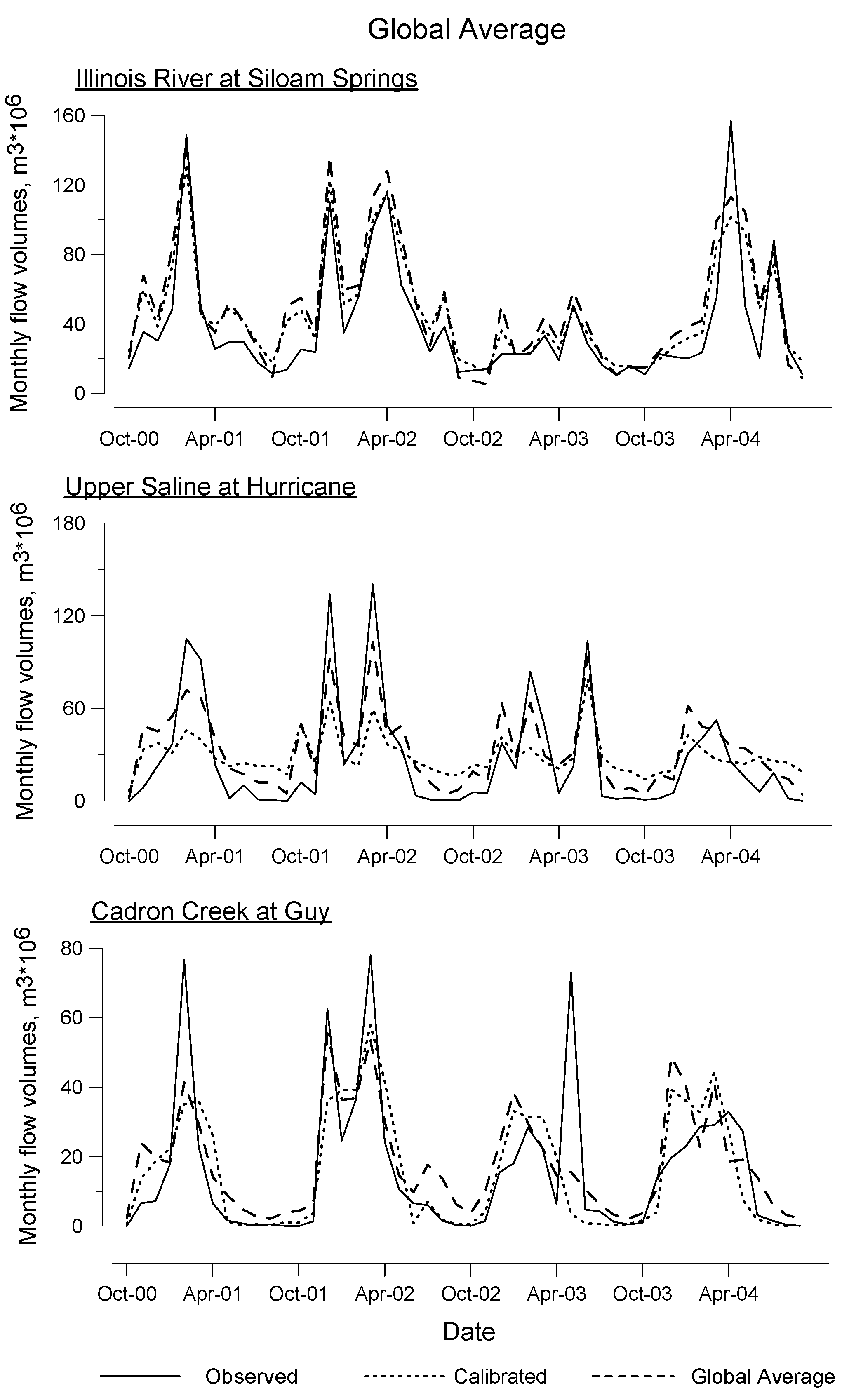
3.1. Global Averaging

Table 3 shows model parameter values as obtained through global averaging. Default values of the parameters are presented for reference purposes. For the Illinois River watershed, the ground water revaporation (GW_REVAP) value obtained from global averaging was close to that obtained through calibration (Table 1) while the global surface runoff lag (surlag) value obtained was closer to the calibrated value for Cadron Creek watershed (Table 1). In some cases, global values obtained differed substantially from calibrated values. For example, while the global average channel hydraulic conductivity (CH_K2) value was 44 mm/hr, the calibrated value for the Cadron Creek watershed was 0.025 (Table 1). Similarly, while the change in curve number (CN2) obtained through global averaging was positive (reflecting an increase), the value obtained through calibration was negative (reflecting a decrease) for all the test watersheds (Table 1).

Table 4 shows model performance statistics obtained using regionalized parameters in comparison to default and calibrated models for the periods October 1998–September 2000, October 2000–September 2004, and for the whole period October 1998–September 2004. Performance obtained using global averaged parameters is shown in column C3. The stations Benton and Sheridan in the Upper Saline watershed did not have data for the period October 1998–September 2000, and thus were only evaluated for the period October 2000–September 2004.

For the Illinois River watershed, NS values obtained using global average parameters ranged between 0.49 and 0.81. In two of the cases, (October 1998–September 2000, Siloam Springs and Savoy) model performance obtained using global average parameters was better than that obtained through calibration. In one case (October 1998–September 2004, Savoy) model performance was very similar for both global averaged and calibrated parameters. For the most part, however, model performance was comparable to calibrated model when global average parameters were used. For example during the period October 2000–September 2004, the NS value obtained from global averaging at Savoy was 0.61 compared to 0.64 obtained through calibration. Similarly, the NS value obtained at the Elm springs station using global averaged parameters was 0.81 compared to 0.90 obtained through calibration (October 1998–September 2000).

Table 3. Model parameter values obtained using global averaging.

Parameter description	Parameter	Default	Global average
Base flow recession factor, days	ALPHA_BF	0.048	0.590
Ground water delay, days	GW_DELAY	31	41
Ground water revaporationh coefficient	GW_REVAP	0.020	0.056
Threshold depth for ground water flow to occur, mm	GWQMN	0.00	14
Deep aquifer recharge fraction	rchrg_dp	0.050	0.272
Threshold depth for revaporation to occur, mm	REVAPMN	1	15
Snow fall temperature, ºC	sftmp	1.0	1.1
Surface runoff lag coefficient, days	surlag	4.00	3.64
Plant uptake compensation factor	EPCO	1.000	0.830
Soil evaporation compensation factor	ESCO	0.950	0.730
Average slope length, m 	SLSUBBSN	Varies1	−2.9%
Curve Number (AMChhII) 	CN2 	Varies2	2.8%
Effective channel hydraulic conductivity, mm/hr	CH_K2	0.5	44.0
Manning's n	ch_n	0.014	0.3‡
Soil albedo	sol_alb	0.100	0.370
Available water capacity, m/m 	SOL_AWC 	Varies3	19.0%

^hReturn flow to root zone. ^hhAntecedent moisture condition. Values represent percent change in parameter. ¹Varies by subbasin; ²Varies by land use and hydrologic soil group; ³Varies by soil type and soil layer. ^‡Values exceeding their reasonable range reset to the maximum for the range.

Table 3. Model parameter values obtained using global averaging.

Parameter description	Parameter	Default	Global average
Base flow recession factor, days	ALPHA_BF	0.048	0.590
Ground water delay, days	GW_DELAY	31	41
Ground water revaporationh coefficient	GW_REVAP	0.020	0.056
Threshold depth for ground water flow to occur, mm	GWQMN	0.00	14
Deep aquifer recharge fraction	rchrg_dp	0.050	0.272
Threshold depth for revaporation to occur, mm	REVAPMN	1	15
Snow fall temperature, ºC	sftmp	1.0	1.1
Surface runoff lag coefficient, days	surlag	4.00	3.64
Plant uptake compensation factor	EPCO	1.000	0.830
Soil evaporation compensation factor	ESCO	0.950	0.730
Average slope length, m 	SLSUBBSN	Varies1	−2.9%
Curve Number (AMChhII) 	CN2 	Varies2	2.8%
Effective channel hydraulic conductivity, mm/hr	CH_K2	0.5	44.0
Manning's n	ch_n	0.014	0.3‡
Soil albedo	sol_alb	0.100	0.370
Available water capacity, m/m 	SOL_AWC 	Varies3	19.0%

^hReturn flow to root zone. ^hhAntecedent moisture condition. Values represent percent change in parameter. ¹Varies by subbasin; ²Varies by land use and hydrologic soil group; ³Varies by soil type and soil layer. ^‡Values exceeding their reasonable range reset to the maximum for the range.

Within the Upper Saline watershed, the model generally performed better with global averaged parameters than with both default and calibrated parameters at the various stations, based on Table 4. For example, global average-based NS for the Hurricane station was 0.73 compared to 0.5 obtained through calibration in the period October 2000–September 2004. Smaller differences in NS values were, however, also observed during the same time period, for example with the Benton station where the NS value obtained through global averaging was 0.56 compared to 0.53 obtained through calibration.

For the Cadron Creek watershed, the NS values obtained using global averaged parameters were the same for the periods October 2000–September 2004, and October 1998–September 2004 (0.55). Model performance in this watershed for the period October 1998–September 2000 was not as good as that obtained using calibrated parameters (0.49 vs. 0.75). However, model performance was better with global values in the period October 2000–September 2004 and over the entire period.

Table 4. Global average and regression-based parameters monthly performance in comparison to performance based on calibrated parameters.

			Nash-Sutcliffe Coefficientŧ
			C1	C2	C3	C4
Time period	Watershed	Station	Default	Calibration	Global average	Regression
Oct. 1998–Sept. 2000	Upper Saline	Benton	--	--	--	--
		Sheridan	--	--	--	--
		Hurricane	−1.96	−0.44	−0.79	−0.95
	Illinois River	Siloam Springs	0.58	0.78	0.81	0.61
		Savoy	0.61	0.64	0.69	0.55
		Elm Springs	−0.20	0.90	0.81	0.82
	Cadron Creek	Guy	−0.39	0.75	0.49	0.63
Oct. 2000–Sept. 2004	Upper Saline	Benton	0.18	0.53	0.56	0.54
		Sheridan	0.41	0.45	0.69	0.61
		Hurricane	0.53	0.50	0.73	0.66
	Illinois River	Siloam Springs	0.31	0.77	0.66	0.75
		Savoy	0.51	0.64	0.61	0.60
		Elm Springs	0.37	0.77	0.49	0.83
	Cadron Creek	Guy	0.28	0.45	0.55	0.53
Oct. 1998–Sept. 2004	Upper Saline	Benton	--	--	--	--
(whole period)		Sheridan	--	--	--	--
		Hurricane	0.42	0.45	0.67	0.60
	Illinois River	Siloam Springs	0.46	0.79	0.74	0.71
		Savoy	0.55	0.64	0.65	0.58
		Elm Springs	0.13	0.85	0.68	0.83
	Cadron Creek	Guy	0.22	0.49	0.55	0.55

^ŧCoefficient can range between −∞ and 1; 0.4 ≤ NS ≤ 0.75—acceptable model performance; NS > 0.75—good performance ([39],[41] (as cited in [42]),[43]). Values closer to 1 are desirable. Blanks (--) imply that data needed for performance evaluation were unavailable.

Table 4. Global average and regression-based parameters monthly performance in comparison to performance based on calibrated parameters.

			Nash-Sutcliffe Coefficientŧ
			C1	C2	C3	C4
Time period	Watershed	Station	Default	Calibration	Global average	Regression
Oct. 1998–Sept. 2000	Upper Saline	Benton	--	--	--	--
		Sheridan	--	--	--	--
		Hurricane	−1.96	−0.44	−0.79	−0.95
	Illinois River	Siloam Springs	0.58	0.78	0.81	0.61
		Savoy	0.61	0.64	0.69	0.55
		Elm Springs	−0.20	0.90	0.81	0.82
	Cadron Creek	Guy	−0.39	0.75	0.49	0.63
Oct. 2000–Sept. 2004	Upper Saline	Benton	0.18	0.53	0.56	0.54
		Sheridan	0.41	0.45	0.69	0.61
		Hurricane	0.53	0.50	0.73	0.66
	Illinois River	Siloam Springs	0.31	0.77	0.66	0.75
		Savoy	0.51	0.64	0.61	0.60
		Elm Springs	0.37	0.77	0.49	0.83
	Cadron Creek	Guy	0.28	0.45	0.55	0.53
Oct. 1998–Sept. 2004	Upper Saline	Benton	--	--	--	--
(whole period)		Sheridan	--	--	--	--
		Hurricane	0.42	0.45	0.67	0.60
	Illinois River	Siloam Springs	0.46	0.79	0.74	0.71
		Savoy	0.55	0.64	0.65	0.58
		Elm Springs	0.13	0.85	0.68	0.83
	Cadron Creek	Guy	0.22	0.49	0.55	0.55

^ŧCoefficient can range between −∞ and 1; 0.4 ≤ NS ≤ 0.75—acceptable model performance; NS > 0.75—good performance ([39],[41] (as cited in [42]),[43]). Values closer to 1 are desirable. Blanks (--) imply that data needed for performance evaluation were unavailable.

Figure 2 shows stream flow hydrographs for selected stations within the test watersheds for the period October 2000–September 2004. For the Illinois River Watershed, the Siloam Springs station was selected as it was located at the watershed outlet. For the Upper Saline Watershed, the Hurricane station was selected as it had the longest period of record. The station at Guy (Cadron Creek Watershed) was used as it was the only station for that watershed. Simulated stream flow obtained using global average parameters in the Illinois River watershed was similar to that obtained through calibration. In both cases (calibrated, global average), simulated stream flow matched the observed values and trends relatively well, based on Figure 2, with deviations mostly being observed during the dry periods. For the Upper Saline watershed, stream flow obtained using global average parameters matched the observed flow slightly better during both peak and low flow periods than did values obtained using calibrated parameters. For the Cadron Creek watershed, the hydrograph obtained using global parameters is very similar to that obtained from the calibrated model, based on Figure 2. In both cases, however, simulated peak flows did not match the observed peak flows very well.

Figure 2. A comparison between global average-based and calibration-based stream flow hydrographs for selected stations within the test watersheds for the period October 2000–September 2004.

Figure 2. A comparison between global average-based and calibration-based stream flow hydrographs for selected stations within the test watersheds for the period October 2000–September 2004.

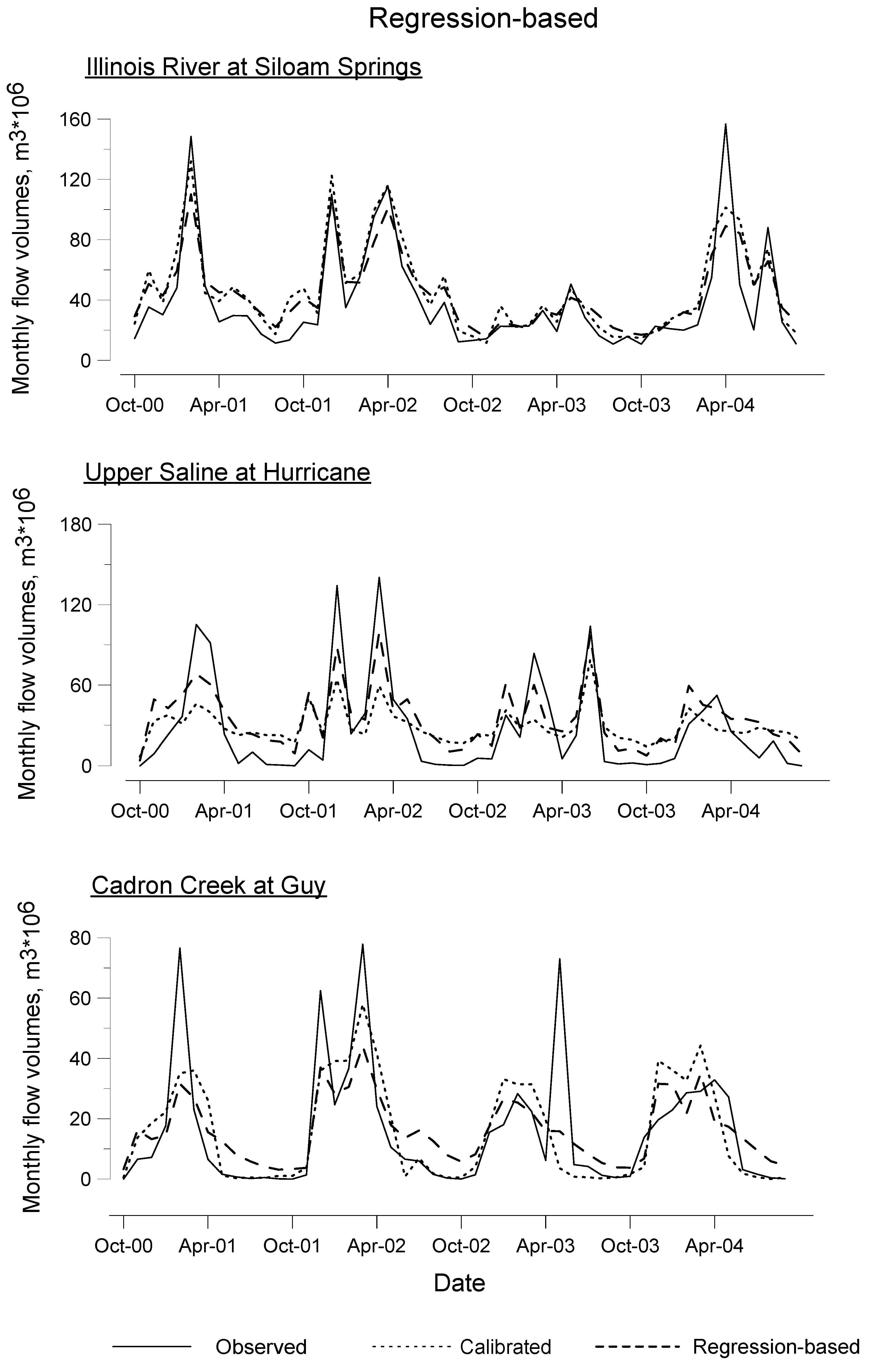
3.2. Regression-based Evaluation

Figure 3 shows regression plots, equations and statistics for model parameters for which significant relationships were obtained. Equations obtained were best for ground water delay (GW_Delay) and soil available water capacity (SOL_AWC), for which R² values obtained were 0.98 and 0.99 (p = 0.04 and 0.0008), respectively. Regressions were worst for the soil evaporation compensation factor (ESCO) for which R² was 0.33 (p = 0.17). For curve number, two possible equations were obtained, one involving the actual curve number value (CN2) and one involving the percentage change in value (CN%). As independent variables were significant in both cases (p = 0.01 and 0.08), and CN2 was highly correlated with CN% (r = 0.857; p = 0.014), the equation involving CN% was used. Values obtained were applied to default HRU values to obtain regression-based curve numbers for each HRU.

A percent change in SLSUBBSN and SOL_AWC values was determined by considering area weighted averages of these parameter values. These weighted averages were used in the regression analyses; values obtained from regression were then compared to area-weighted default values and the percentage change of the parameter from the default value computed. The percent changes in parameter values obtained were then used to calculate regression-based values for the HRUs.

Table 5 shows model parameters as obtained using regression. Default values are presented for reference purposes. Where no suitable equation was found, the corresponding global average value was used. These values were input into the SWAT model for the respective watersheds. Model runs were then performed and performance measures computed as previously described. For Cadron Creek watershed, the regression-based base flow recession factor obtained was 1.05, which exceeded the upper limit (1) for that parameter. This value was reset to one (1) so that parameter bounds were not exceeded. Values obtained for GW_DELAY were close to those obtained through calibration for both the Illinois and Upper Saline watersheds (Table 1). As with the global averages, most of the other regression-based values differed from those obtained through calibration.

Performance statistics for each watershed as obtained using regression-based parameters are also shown in Table 4 (column C4). In general, the model performed well when regression-based parameters were used with NS values ranging between 0.53 and 0.83. Generally, model performance obtained using regression-based parameters was comparable to that obtained through calibration, based on Table 4. Model performance sometimes exceeded that obtained using calibrated parameters, for example with the Upper Saline watersheds for the period October 2000–September 2004. The model with regression-based parameters also consistently outperformed the default model outputs in all the periods evaluated, based on Table 4.

Figure 3. Regression plots, equations and statistics for model parameters for which significant relationships were obtained. Dotted lines represent 95% confidence intervals. R² denotes the coefficient of determination, 0 ≤ R² ≤ 1. P denotes the probability of obtaining a value of the test statistic (in this case F) that is greater than that observed.

Figure 3. Regression plots, equations and statistics for model parameters for which significant relationships were obtained. Dotted lines represent 95% confidence intervals. R² denotes the coefficient of determination, 0 ≤ R² ≤ 1. P denotes the probability of obtaining a value of the test statistic (in this case F) that is greater than that observed.

Table 5. Model parameter values obtained using regression.

			Regression-based values
Parameter description	Parameter	Default	Illinois River	Upper Saline	Cadron Creek
Base flow recession factor, days	ALPHA_BF	0.048	0.610	0.640	1.000‡
Ground water delay, days	GW_DELAY	31	84	71	72
Ground water revaporationh coefficient	GW_REVAP	0.020	0.056*	0.056*	0.056*
Threshold depth for ground water flow to occur, mm	GWQMN	0	14*	14*	14*
Deep aquifer recharge fraction	rchrg_dp	0.050	0.272*	0.272*	0.272*
Threshold depth for revaporation to occur, mm	REVAPMN	1	15*	15*	15*
Snow fall temperature, ºC	sftmp	1.0	1.1*	1.1*	1.1*
Surface runoff lag coefficient, days	surlag	4.00	3.64*	3.64*	3.64*
Plant uptake compensation factor	EPCO	1.000	0.830*	0.830*	0.830*
Soil evaporation compensation factor	ESCO	0.950	0.530	0.790	0.570
Average slope length, m	SLSUBBSN	Varies1	−16.0%	−10.0%	0.0%
Curve Number (AMChh II)	CN2 	Varies2	−24.2%	−0.7%	−24.0%
Effective channel hydraulic conductivity, mm/hr	CH_K2	0.5	44.0*	44.0*	44.0*
Manning’s n	ch_n	0.014	0.3*‡	0.3*‡	0.3*‡
Soil albedo	sol_alb	0.100	0.370*	0.370*	0.370*
Available water capacity, m/m	SOL_AWC	Varies3	−33.0%	−20.0%	50.0%

^hReturn flow to root zone. ^hhAntecedent moisture condition. Values represent percent change in parameter. ¹Varies by subbasin; ²Varies by land use and hydrologic soil group; ³Varies by soil type and soil layer. ^‡Values exceeding their reasonable range reset to the maximum for the range. ^*Global average values used as no suitable equation was found.

Table 5. Model parameter values obtained using regression.

			Regression-based values
Parameter description	Parameter	Default	Illinois River	Upper Saline	Cadron Creek
Base flow recession factor, days	ALPHA_BF	0.048	0.610	0.640	1.000‡
Ground water delay, days	GW_DELAY	31	84	71	72
Ground water revaporationh coefficient	GW_REVAP	0.020	0.056*	0.056*	0.056*
Threshold depth for ground water flow to occur, mm	GWQMN	0	14*	14*	14*
Deep aquifer recharge fraction	rchrg_dp	0.050	0.272*	0.272*	0.272*
Threshold depth for revaporation to occur, mm	REVAPMN	1	15*	15*	15*
Snow fall temperature, ºC	sftmp	1.0	1.1*	1.1*	1.1*
Surface runoff lag coefficient, days	surlag	4.00	3.64*	3.64*	3.64*
Plant uptake compensation factor	EPCO	1.000	0.830*	0.830*	0.830*
Soil evaporation compensation factor	ESCO	0.950	0.530	0.790	0.570
Average slope length, m	SLSUBBSN	Varies1	−16.0%	−10.0%	0.0%
Curve Number (AMChh II)	CN2 	Varies2	−24.2%	−0.7%	−24.0%
Effective channel hydraulic conductivity, mm/hr	CH_K2	0.5	44.0*	44.0*	44.0*
Manning’s n	ch_n	0.014	0.3*‡	0.3*‡	0.3*‡
Soil albedo	sol_alb	0.100	0.370*	0.370*	0.370*
Available water capacity, m/m	SOL_AWC	Varies3	−33.0%	−20.0%	50.0%

^hReturn flow to root zone. ^hhAntecedent moisture condition. Values represent percent change in parameter. ¹Varies by subbasin; ²Varies by land use and hydrologic soil group; ³Varies by soil type and soil layer. ^‡Values exceeding their reasonable range reset to the maximum for the range. ^*Global average values used as no suitable equation was found.

Figure 4 shows graphical plots for selected stations within the watershed. Simulated stream flow obtained using regression-based parameters in the Illinois watershed compared well to that obtained through calibration, based on Figure 4. In both cases, calibrated stream flow matched the observed values and trends relatively well. For the Upper Saline watershed, stream flow obtained using regression-based parameters was comparable to that obtained through calibration. In both cases, the model tended to overestimate flow during base flow conditions. Simulations obtained using regression-based parameters matched the observed peak flows somewhat better than did values obtained using calibrated parameters. This would explain why better performance statistics were obtained using regression-based parameters than what was obtained during calibration. For the Cadron Creek watershed, the hydrograph obtained through calibration was better than that obtained using regression-based parameters, particularly during low flow periods. However, where deviations from observed values were large, these were generally more pronounced when calibrated parameters were used than when regression-based parameters were used, thus the lower NS values obtained for calibrations than for regression-based simulations.

Figure 4. A comparison between regression-based and calibration-based stream flow hydrographs for selected stations within the test watersheds for the period October 2000– September 2004.

Figure 4. A comparison between regression-based and calibration-based stream flow hydrographs for selected stations within the test watersheds for the period October 2000– September 2004.

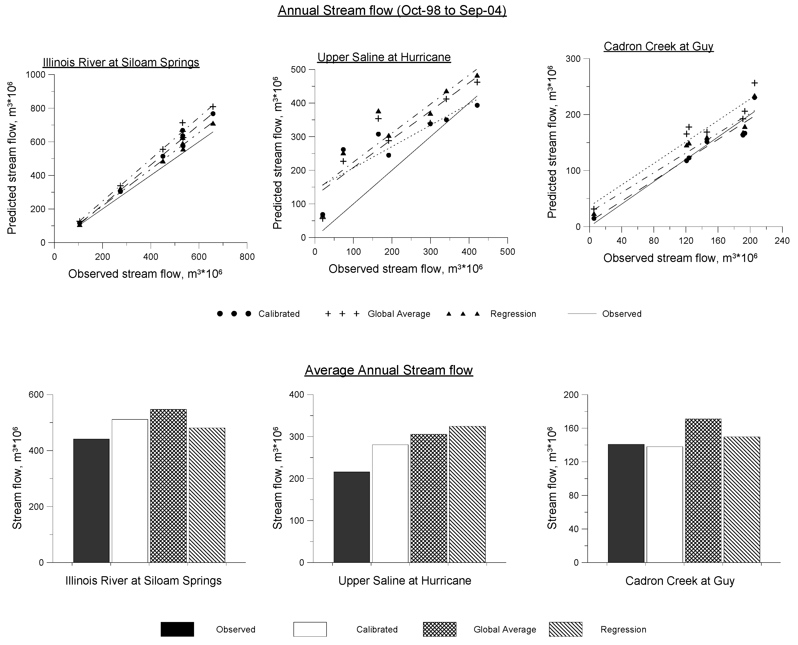
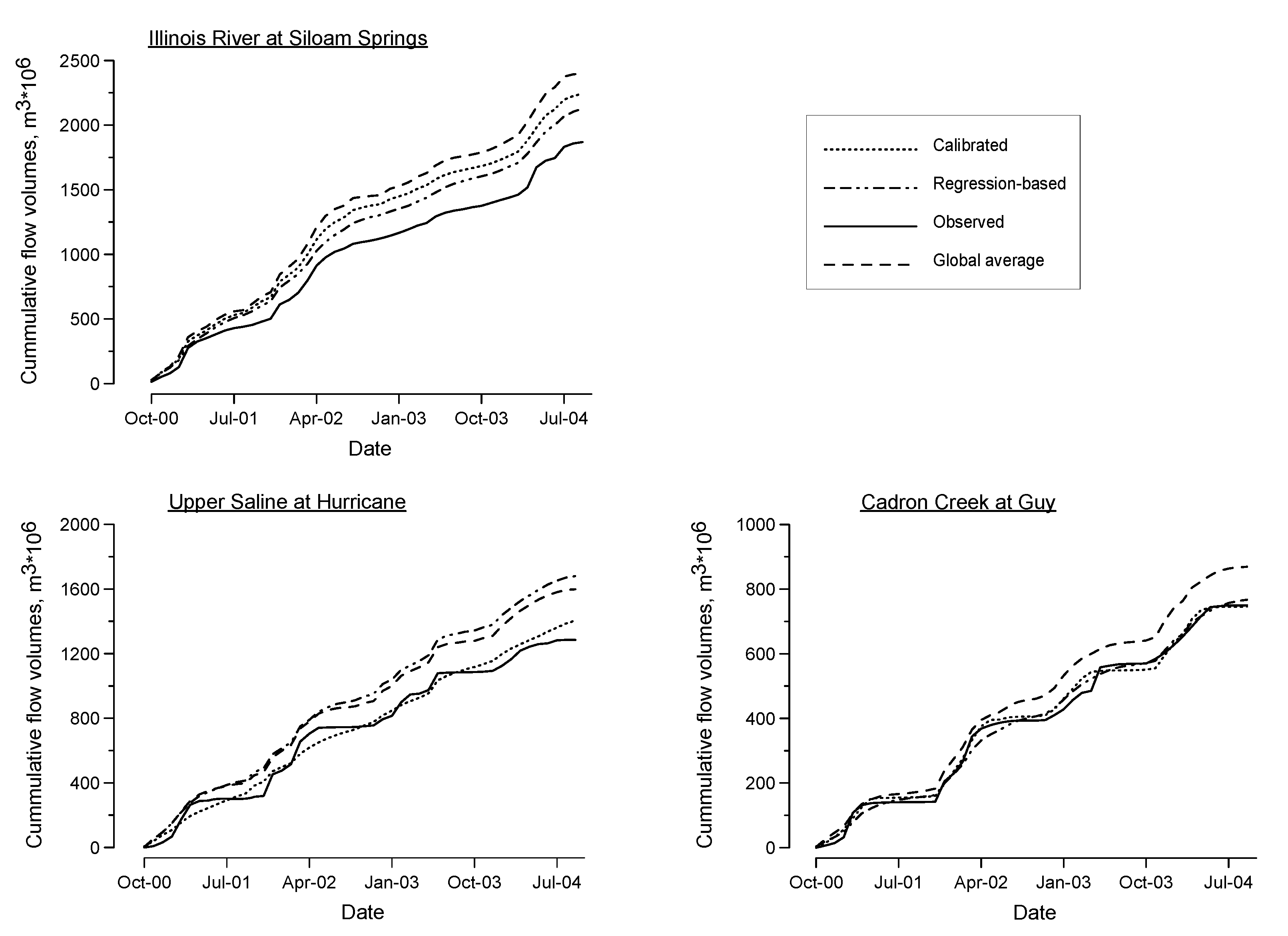
3.3. Performance Analyses of Parameter Regionalization Methods

In general, the best (highest) NS coefficients and (lowest) Dv values were obtained using calibration parameters (Table 4 and Table 6). With the exception of Upper Saline at Hurricane (October 1998– September 2000) and Upper Saline at Benton (annual) model performance obtained using regression-based parameters ranged between acceptable and good, based on published criteria [41] (as cited in [42]),[43]. Using regression-based parameters, 29% of the NS values obtained were greater than 0.75 (indicating good model performance) compared with 42% obtained through calibration and 8% obtained through global averaged parameters. In 10 out of 24 cases, NS and Dv values obtained through regression-based parameters were better than those obtained using calibrated parameters. This was especially true when performance was considered on an annual basis (Table 6). For example, the NS and Dv values obtained at the Elm Springs gauge in the Illinois River watershed using regression-based parameters were 0.94 and 0.10, respectively, while corresponding values obtained through calibration were 0.79 and 0.16 respectively. This suggests that regression-based parameters could provide suitable alternatives where calibrations were not possible due to paucity of data.

Table 6. Annual NS and Dv values for the period October 1998 to September 2004.

		Nash-Sutcliffe Coefficientŧ / Dv*
Watershed	Station	Calibration	Global Average	Regression
Upper Saline	Benton†	0.16/0.31	−0.51/0.43	−1.07/0.51
	Sheridan	0.87/0.09	0.61/0.28	0.44/0.34
	Hurricane	0.50/0.30	0.38/0.41	0.40/0.50
Illinois River	Siloam Springs	0.78/0.16	0.55/0.24	0.92/0.09
	Savoy	0.68/0.1	0.48/0.18	0.82/0.04
	Elm Springs	0.79/0.16	0.55/0.25	0.94/0.10
Cadron Creek	Guy	0.92/−0.02	0.69/0.21	0.89/0.06

^ŧCoefficient can range between −∞ and 1; 0.4 ≤ NS ≤ 0.75—acceptable model performance; NS > 0.75—good performance ([39],[41] (as cited in [42]),[43]). Values closer to 1 are desirable. ^*Deviation (-1 ≤ Dv ≤ 1, low values preferable). ^†Values for Benton represent the period 2000–2004 as this station did not have data for the preceding period.

Table 6. Annual NS and Dv values for the period October 1998 to September 2004.

		Nash-Sutcliffe Coefficientŧ / Dv*
Watershed	Station	Calibration	Global Average	Regression
Upper Saline	Benton†	0.16/0.31	−0.51/0.43	−1.07/0.51
	Sheridan	0.87/0.09	0.61/0.28	0.44/0.34
	Hurricane	0.50/0.30	0.38/0.41	0.40/0.50
Illinois River	Siloam Springs	0.78/0.16	0.55/0.24	0.92/0.09
	Savoy	0.68/0.1	0.48/0.18	0.82/0.04
	Elm Springs	0.79/0.16	0.55/0.25	0.94/0.10
Cadron Creek	Guy	0.92/−0.02	0.69/0.21	0.89/0.06

^ŧCoefficient can range between −∞ and 1; 0.4 ≤ NS ≤ 0.75—acceptable model performance; NS > 0.75—good performance ([39],[41] (as cited in [42]),[43]). Values closer to 1 are desirable. ^*Deviation (-1 ≤ Dv ≤ 1, low values preferable). ^†Values for Benton represent the period 2000–2004 as this station did not have data for the preceding period.

In general, NS values obtained using global averaged parameters were mostly in the acceptable range. Values of NS obtained using global parameters exceeded those obtained using both calibration and regression-based parameters 9 and 12 out of 24 times respectively. However, NS values obtained using global parameters exceeded the acceptable range 2 out of 24 times, compared to 10 and 7 out of 24 times for calibrated and regression-based parameters respectively. For example, the NS value obtained at the Siloam Springs gauge during October 1998 to September 2000 was 0.81 when global parameters were used, compared to 0.78 and 0.61 obtained using calibrated and regression based parameters for the same time period, respectively. Values not meeting either criterion (acceptable or good) were comparable across the methods. At the Hurricane gauge, for example, monthly NS values were less than zero for all methods; annual NS values obtained at the Benton gauge were also negative for both global average and regression-based methods, while calibrated NS values showed unsatisfactory (NS < 0.4) model performance. In all cases NS values obtained using global averaged parameters were better than those obtained using the default model. This suggests that global averaged parameters could also be used to provide alternative parameters where calibrations cannot be conducted. The global averaged parameters have the potential to provide better model performance than that obtained with the default model, making it a method worth considering.

Figure 5 shows a comparison of cumulative plots as obtained using the various regionalization methods for the period October 2000–September 2004. A shorter period was used for these plots so as to ensure the cumulative plots were legible. The particular period was selected because it was the period for which data availability was consistent among stations. For the Illinois River watershed results obtained using both regression-based and global averaged parameters were comparable to those obtained using calibration parameters. However, stream flow obtained using global parameters was higher than that obtained through calibration, while stream flow obtained using regression-based parameters was lower. In all cases (calibration, global average, regression-based) the model overestimated stream flow, when compared with observed data, with global average parameters having the highest level of overestimation. This is attributable to high curve numbers associated with global parameters, as global averaging called for a 2.8% increase in curve numbers.

For the Upper Saline watershed, regression-based and global-averaged parameters resulted in approximately similar patterns. These also closely matched the trends in the observed data. With regard to flow volumes, however, values obtained using calibration matched observed values most closely; the model tended to overestimate stream flow when either global averaged or regression-based parameters were used, this being particularly so during dry periods (Figure 2 and Figure 4). For the Cadron Creek watershed, plots obtained using regression-based parameters closely matched those obtained using calibration parameters; both plots closely matched observed data. The plot obtained using global averaged parameters showed deviation from all the other plots. This was because the model tended to overestimate low flows when global parameters were used, yet observed underestimation of peak flows was not sufficient to compensate for this overestimation (Figure 2).

Figure 6 shows scatter plots for annual stream flows for the period October 1998 to September 2004 (top) and a comparison of average annual stream flow values (bottom) as obtained using the various regionalization methods. For the Cadron Creek watershed, simulated stream flow obtained using regression-based parameters matched observed data relatively well, while that obtained using global average parameters overestimated the stream flow. For the Illinois River watershed, regression-based stream flow matched observed stream flow well for low flows but deviated during high flow conditions. The model, however, overestimated annual stream flows in this watershed when global average parameters were used. Plots obtained for the Upper Saline watershed showed consistent over estimation by all regionalization methods. Overall, results obtained for annual performance were consistent with those obtained from assessments at the monthly time-step.

Figure 5. Inter-comparison of stream flow hydrographs as obtained using the various regionalization methods, and calibration for the period October 2000–September 2004.

Figure 5. Inter-comparison of stream flow hydrographs as obtained using the various regionalization methods, and calibration for the period October 2000–September 2004.

Figure 6. Scatter plots for annual stream flow volumes for the period October 1998 to September 2004 (top) and comparison of average annual volumes (bottom) as obtained using the various regionalization methods.

Figure 6. Scatter plots for annual stream flow volumes for the period October 1998 to September 2004 (top) and comparison of average annual volumes (bottom) as obtained using the various regionalization methods.

4. Conclusions

This study evaluated the use of regionalization as a means of obtaining SWAT model parameters for use in ungauged watersheds. The study evaluated two regionalization methods: global average and regression-based estimates in terms of their predictive abilities using measured data from three different watersheds in Arkansas.

Model performance obtained using both the global averaged and regression-based parameters was comparable to that obtained through calibration. Monthly Nash-Sutcliffe efficiencies for stream flow varied between 0.53–0.83 when regression-based parameters were used, and 0.49–0.81 when global averaged parameters were used, respectively, compared with values of 0.45–0.90 obtained through calibration. Annual Nash-Sutcliffe efficiencies varied between 0.40–0.94 for regression-based parameters and 0.38–0.69 for global averaged parameters compared with values of 0.50–0.92 obtained through calibration. Model performance obtained with global average parameters sometimes equaled or exceeded the performance obtained using parameter values from either calibration or regression-based estimates. However, watershed response predictions obtained using global parameters were mostly in the acceptable (0.4 ≤ NS ≤ 0.75) range. In comparison, good model efficiencies (measured as NS values greater than 0.75) were obtained for a greater number of data sets using calibration and regression-based parameters than using global average parameters.

Examination of graphical plots showed that model performance was comparable across the methods when considered on a monthly basis. Cumulative and average annual plots, however, showed that the model tended to overestimate stream flow, regardless of the method. The amount of overestimation was highest where global average parameters were used.

Overall, suitable model performance was obtained using both global averaged and regression-based methods, based on the evaluation of model performance. It is not clear why any one method worked better for some watersheds but not for others. In both cases, however, model performance obtained through regionalization was better than that obtained from using default parameters, thus further highlighting their usefulness in ungauged watersheds. Results suggest that better model performance can be obtained by using regression-based parameters than by using global averaged parameters. Development of regression-based parameters requires more data and more time involvement than does development of global averaged parameters, more so because watershed characteristics are involved. Further, suitable statistical software is needed in the regression-based method, whereas obtaining global averages can be accomplished with a standard spreadsheet. Regression-based parameters have often been found to work best for lumped models with few parameters. This study showed that suitable regression-based parameters can also be obtained for distributed parameter models provided there were sufficient data with which to develop relationships.

The regionalized model parameters were obtained using data from watershed situated at various locations throughout the state of Arkansas. These parameters were tested on three gauged watersheds in Arkansas, one of which was independent of the seven that had been used to derive the regional parameter sets. Overall, the model performed well when these parameters were used on the test watersheds, thus, we are confident that the parameters would give satisfactory results when used in Arkansas’ ungaged watersheds. Results might, however, not be directly transferable to other watersheds outside of Arkansas. The methodologies so developed are, however, applicable in other regions where there is a need to regionalize model parameters. In general, results suggest that it is possible to obtain regionalized SWAT model parameter sets for use in watersheds for which calibrations and validation cannot be conducted due to lack of monitoring data.

References

1. Arnold, J.G.; Srinivasan, R.; Muttiah, R.S.; Williams, J.R. Large area hydrologic modeling and assessment—Part 1: Model development. J. Am. Water Resour. Assoc. 1998, 34, 73–89. [Google Scholar] [CrossRef]
2. Bosch, D.D.; Bingner, R.L.; Theurer, F.D.; Felton, G. Evaluation of the AnnAGNPS water quality model. ASAE Paper 98-2195. American Society of Agricultural Engineers (ASAE): St. Joseph, MI, USA, 1998. [Google Scholar]
3. Bouraoui, F.; Dillaha, T.A. ANSWERS-2000: Runoff and sediment transport model. J. Environ. Eng. 1996, 122, 493–502. [Google Scholar] [CrossRef]
4. Johanson, R.C.; Imhoff, J.D.; Davis, H.H., Jr. Users’ Manual for Hydrological Simulation Program—Fortran (HSPF); EPA-600/9-80-015; Environmental Research Laboratory: Athens, GA, USA, 1980. [Google Scholar]
5. Bicknell, B.R.; Imhoff, J.C.; Kittle, J.J.L.; Jobs, T.H.; Donigian, A.S. Hydrological Simulation Program—FORTRAN: HSPF Version 12 User’s Manual; Aqua Terra Consultants: Mountain View, CA, USA, 2001. [Google Scholar]
6. Jarboe, J.E.; Hann, C.T. Calibrating a water yield model for small ungauged watersheds. Water Resour. Res. 1974, 10, 256–262. [Google Scholar] [CrossRef]
7. Karlinger, M.R.; Guertin, D.P.; Troutman, B.M. Regression estimates for topological—hydrograph input. J. Water Resour. Plan. Man. 1988, 114, 446–456. [Google Scholar] [CrossRef]
8. Vogel, R.M. Regional Calibration of Watershed Models. In Watershed Models; Singh, V.P., Frevert, D.K., Eds.; CRC Press: Boca Raton, FL, USA, 2006; Chapter 3; pp. 47–71. [Google Scholar]
9. Bloschl, G.; Sivapalan, M. Scale Issues in Hydrological Modeling—a Review. Hydrol. Process. 1995, 9, 251–290. [Google Scholar] [CrossRef]
10. Merz, R.; Bloschl, G. Regionalisation of catchment model parameters. J. Hydrol. 2004, 287, 95–123. [Google Scholar] [CrossRef]
11. Magette, W.L.; Shanholtz, V.O.; Carr, J.C. Estimating selected parameters for the Kentucky Watershed Model from watershed characteristics. Water Resour. Res. 1976, 12, 472–476. [Google Scholar] [CrossRef]
12. Servat, E.; Dezetter, A. Rainfall-Runoff Modeling and Water Resources Assessment in Northwestern Ivory-Coast—Tentative Extension to Ungauged Catchments. J. Hydrol. 1993, 148, 231–248. [Google Scholar] [CrossRef]
13. Post, D.A.; Jakeman, A.J. Relationships between catchment attributes and hydrological response characteristics in small Australian mountain ash catchments. Hydrol. Process. 1996, 10, 877–892. [Google Scholar] [CrossRef]
14. Post, D.A.; Jakeman, A.J. Predicting the daily streamflow of ungauged catchments in SE Australia by regionalising the parameters of a lumped conceptual rainfall-runoff model. Ecol. Model. 1999, 123, 91–104. [Google Scholar] [CrossRef]
15. Vandewiele, G.L.; Elias, A. Monthly Water-Balance of Ungauged Catchments Obtained by Geographical Regionalization. J. Hydrol. 1995, 170, 277–291. [Google Scholar] [CrossRef]
16. Kokkonen, T.S.; Jakeman, A.J.; Young, P.C.; Koivusalo, H.J. Predicting daily flows in ungauged catchments: Model regionalization from catchment descriptors at the Coweeta Hydrologic Laboratory, North Carolina. Hydrol. Process. 2003, 17, 2219–2238. [Google Scholar] [CrossRef]
17. Schmidt, J.; Hennrich, K.; Dikau, R. Scales and similarities in runoff processes with respect to geomorphometry. Hydrol. Process. 2000, 14, 1963–1979. [Google Scholar] [CrossRef]
18. Seibert, J. Regionalization of parameters for a conceptual rainfall-runoff model. Agr. Forest Meteorol. 1999, 98-99, 279-293. [Google Scholar]
19. Watershed Boundary Dataset. Coordinated Effort between the United States Department of Agriculture-Natural Resources Conservation Service (USDA-NRCS),the United States Geological Survey (USGS),and the Environmental Protection Agency (EPA). (Created from a Variety of Sources from Each State and Aggregated into a Standard National Layer for Use in Strategic Planning and Accountability). Available online: http://datagateway.nrcs.usda.gov (accessed on 18 October  2007).
20. Chaubey, I.; Matlock, M.; Costello, T.; Cooper, C.; White, K. GIS Database Development and Watershed Modeling in Arkansas Priority Watersheds; Final report submitted to Arkansas Soil and Water Conservation Commission. Project No. 04-120. In 2004.
21. White, K.L.; Chaubey, I. Sensitivity analysis, calibration, and validations for a multisite and multivariable SWAT model. J. Am. Water Resour. Assoc. 2005, 41, 1077–1089. [Google Scholar] [CrossRef]
22. Chaubey, I.; Matlock, M.; Garg, V. GIS Database Development and Watershed Modeling in Arkansas Priority Watersheds; Final Report submitted to the Arkansas Soil and Water Conservation Commission. Project No. 02-1400. In 2006.
23. Arnold, J.G.; Fohrer, N. SWAT2000: Current capabilities and research opportunities in applied watershed modelling. Hydrol. Process. 2005, 19, 563–572. [Google Scholar] [CrossRef]
24. Jayakrishnan, R.; Srinivasan, R.; Santhi, C.; Arnold, J.G. Advances in the application of the SWAT model for water resources management. Hydrol. Process. 2005, 19, 749–762. [Google Scholar] [CrossRef]
25. Gitau, M.W.; Veith, T.L.; Gburek, W.J.; Jarrett, A.R. Watershed level best management practice selection and placement in the town brook watershed, New York. J. Am. Water Resour. Assoc. 2006, 42, 1565–1581. [Google Scholar] [CrossRef]
26. Migliaccio, K.W.; Chaubey, I.; Haggard, B.E. Evaluation of landscape and instream modeling to predict watershed nutrient yields. Environ. Model. Softw. 2007, 22, 987–999. [Google Scholar] [CrossRef]
27. Miller, S.N.; Semmens, D.J.; Goodrich, D.C.; Hernandez, M.; Miller, R.C.; Kepner, W.G.; Guertin, D.P. The Automated Geospatial Watershed Assessment tool. Environ. Model. Softw. 2007, 22, 365–377. [Google Scholar] [CrossRef]
28. Gitau, M.W.; Veith, T.L.; Gburek, W.J. Farm-level optimization of BMP placement for cost-effective pollution reduction. Trans. ASAE 2004, 47, 1923–1931. [Google Scholar] [CrossRef]
29. Cerucci, M.; Conrad, J.M. The use of binary optimization and hydrologic models to form Riparian buffers. J. Am. Water Resour. Assoc. 2003, 39, 1167–1180. [Google Scholar] [CrossRef]
30. Neitsch, S.L.; Arnold, J.G.; Kiniry, T.R.; Williams, J.R. Soil and Water Assessment Tool. Theoretical Documentation; Texas Water Resources Institute: College Station, TX, USA, 2005. [Google Scholar]
31. Water Pollution Control Federation. Design and Construction of Sanitary and Storm Sewers. Manual of Practice 9. In ASCE Manual of Engineering practice; Water Pollution Control Federation: Washington, DC, USA, 1969. [Google Scholar]
32. Lane, L.J. Transmission Losses. In Soil Conservation Service. National Engineering Handbook; U.S. Government Printing Office: Washington, DC, USA, 1983; pp. 19-11–19-21. [Google Scholar]
33. Kresse, T.M.; Fazio, J.A. Pesticides, Water Quality and Geochemical Evolution of Ground Water in the Alluvial Aquifer, Bayou Bartholomew Watershed, Arkansas; Arkansas Ambient Ground-Water Monitoring Program; Arkansas Department of Environmental Quality: Little Rock, AR, USA, 2002. [Google Scholar]
34. Neitsch, S.L.; Arnold, J.G.; Kiniry, T.R.; Williams, J.R. Soil and Water Assessment Tool. User’s Manual; Texas Agricultural Experiment Station: Temple, TX, USA, 2001. [Google Scholar]
35. Mason, C.H.; Perreault, W.D. Collinearity, power, and interpretation of multiple-regression analysis. J. Market. Res. 1991, 28, 268–280. [Google Scholar] [CrossRef]
36. Nash, J.E.; Sutcliffe, J.V. River flow forecasting through conceptual models: Part 1. A discussion of principles. J. Hydrol. 1970, 10, 282–290. [Google Scholar]
37. Martinez, J.; Rango, A. Merits of statistical criteria for the performance of hydrological models. Water Resour. Bull. 1989, 25, 421–432. [Google Scholar] [CrossRef]
38. Gassman, P.W.; Reyes, M.R.; Green, C.H.; Arnold, J.G. The soil and water assessment tool: Historical development, applications, and future research directions. Trans. ASABE 2007, 50, 1211–1250. [Google Scholar] [CrossRef]
39. Moriasi, D.N.; Arnold, J.G.; Van Liew, M.W.; Bingner, R.L.; Harmel, R.D.; Veith, T.L. Model evaluation guidelines for systematic quantification of accuracy in watershed simulations. Trans. ASABE 2007, 50, 885–900. [Google Scholar] [CrossRef]
40. Engel, B.; Storm, D.; White, M.; Arnold, J.; Arabi, M. A hydrologic/water quality model application protocol. J. Am. Water Resour. Assoc. 2007, 43, 1223–1236. [Google Scholar] [CrossRef]
41. Popov, E.G. Gidrologicheskie Prognozy (Hydrological Forecasts); Gidrometeoizdat: Leningrad, Russia, 1979. [Google Scholar]
42. Van Liew, M.W.; Garbrecht, J. Hydrologic simulation of the Little Washita river experimental watershed using SWAT. J Am.Water Resour. Assoc. 2003, 39, 413–426. [Google Scholar] [CrossRef]
43. Ramanarayanan, T.S.; Williams, J.R.; Dugas, W.A.; Hauck, L.M.; McFarland, A.M.S. Using APEX to Identify Alternative Practices for Animal Waste Management; ASAE Paper 97-2209; American Society of Agricultural Engineers (ASAE): St. Joseph, MI, USA, 1997. [Google Scholar]
44. Donigan, A.S.; Love, J.T. Sediment Calibration Procedures and Guidelines for Watershed Modeling. In WEF TMDL 2003 Specialty Conference; WEF-CDROM: Chicago, IL, USA, 2003. [Google Scholar]
45. Sorooshian, S.; Gupta, V.K. Model Calibration. In Computer Models of Watershed Hydrology; Singh, V.P., Ed.; Water Resources Publications: Highlands Ranch, CO, USA, 1995. [Google Scholar]
46. Jacomino, V.M.F.; Fields, D.E. A critical approach to the calibration of a watershed model. J. Am. Water Resour. Assoc. 1997, 33, 143–154. [Google Scholar] [CrossRef]