Article

The Occurrence of Cold Spells in the Alps Related to ClimateChange

1
Department of General Physics “Amedeo Avogadro”, University of Torino, Via Pietro Giuria 1 10125, Torino (TO), Italy
2
Department of Environmental Science and Engineering, Severe Storm Research Center and Center for Climate/Environment Change Prediction Research, Ewha Womans University, Seoul 120-750, Korea
*
Author to whom correspondence should be addressed.
Water 2010, 2(3), 363-380; https://doi.org/10.3390/w2030363
Submission received: 23 June 2010 / Revised: 27 July 2010 / Accepted: 27 July 2010 / Published: 2 August 2010

Abstract

:
Climate change is not only a likely prospect for the end of this century, but it is already occurring. Part of the changes will include global warming and increasing temperature variability, both at global and regional scales. This increased variability was investigated in this paper from the point of view of the occurrence of cold spells in the Alps in the future climate (2071–2100), compared with the present climate (1961–1990). For this purpose, a regionalisation of the climate change effects was performed within the Alps. To avoid possible errors in the estimate of the 2m air temperature, the analysis was performed on the soil surface temperature. To get realistic values for this variable, a land surface scheme, UTOPIA, has been run on the selected domain, using the output of the Regional Climate Model (RegCM3) simulations as the driving force. The results show that, in general, the number of cold breaks is decreasing over the Alps, due to the temperature increment. However, there are certain zones where the behaviour is more complicated. The analysis of the model output also allowed a relationship to be found between the number of cold breaks and their duration. The significance of these results over the whole area was assessed.

Graphical Abstract

1. Introduction

There is a general consensus by the scientific community about the importance of the land surface processes as a key component of the climatic system. The soil is very important because of its role in regulating the atmospheric energy and water balance, and consequently, affecting its dynamics, providing both energy and water vapour. Slightly different conditions in some parameters, such as the soil moisture and temperature, can affect the stability of the boundary layer and, as a consequence, the whole troposphere. The stability of the atmosphere is a fundamental point in the description of convective phenomena, which determines the formation of cumulus clouds and eventually precipitation [1].
The soil, possessing a greater capacity to store both energy and water, has a larger response time than the atmosphere to the external forcings. Energy flux input for the soil is due to the incoming net radiation from the above atmospheric layers (or from vegetation, ice or snow). This input, when positive, increases the soil temperature, transporting energy from the surface to the deeper layers (conductive heat flux). The soil surface loses part of this positive energy flux by generating turbulent heat fluxes directed towards the atmosphere: the direct warming constitutes the sensible heat flux, while the latent energy involved in the liquid water evaporation constitutes the latent heat flux [1].
In the recent years, the changes in the frequency and intensity of climatic extremes, which are likely to accompany global warming, have been approached by the scientific community [2]. Both on global and regional basis, there are convincing evidences of such extremes [3]. According to the IPCC emission scenarios [4], many Global Climate Models (GCMs) are producing climate simulations to approach, among many other problems, the study of the occurrence of warm and cold spells during the 21st century [5]. Current computing resources allow the results of global simulations to be downscaled to the regional scale by using limited area models [6,7], and the studies of climate extreme sequences are carried out with higher resolution [8,9].
In the present work, attention is focused on the Po Valley and Alpine Area. The goal of this work is to study the length and the frequency of cold spells in soil temperature of the Alpine Area in relation to climate change. Thus, the extremes studied in this case are the frequency and the length of cold breaks. The analysis was carried out by considering the soil temperature, since this variable exhibits less noise than air temperature in its time series, due to the fact that the soil specific heat capacity is greater than that of the air.
This kind of studies is important because users of climate information are often concerned about the high frequency of weather extremes taking place in a particular region [10], especially because there is a wide consensus among climatologists that climate change could result in an increased variability [11]. In addition, the Alpine Area is a key region for Europe, since it is the source of many important rivers [12], and climate change there can affect many people. Climate change in the Alps has produced an increment of temperature which is almost double with respect to the trends observed at global scale, meaning that the climate system in this region possesses a large number of feedbacks [13]. The literature about this kind of studies is extensive, and an example of the studies on that can be found in [14].
The technique adopted in the context of this work is a time series approach where the number of consecutive days of cold temperature (a definition of this concept is given in section 3) is calculated, and the number of such events is analysed so that it is possible to determine a different kind of response to climate change of different alpine locations, or global responses over the whole area under the investigation of this study.
The data used to employ the technique above mentioned come from a chain of simulations. A regional climate model, RegCM3, which used the output of a global climate model, HadAMH, as its input was driven by the present (1961–1990) and future (2071–2100) climate scenarios, was used as source of meteorological data at screen level. Subsequently, these were used to drive a land surface scheme, the UTOPIA, at each grid point of the target area, and the data of daily soil temperatures were extracted from the output database.
Section 2 describes in detail the models involved in this study and the specific data used in the work; Section 3 gives a description of the working methodology; and Section 4 lists and discusses the results.

2. Models Involved in the Study

Only the land surface scheme UTOPIA (University of TOrino land Process Interaction with Atmosphere), described in Section 2.2, was directly used for this study. However, as specified in Section 3, the input data used by UTOPIA came from a simulation carried out by other researchers [15,16,17] using the Regional Climate Model RegCM3, therefore this model is also described in section 2.1. The other relevant dataset used by UTOPIA and RegCM3 is discussed in the section 3.

2.1. RegCM3

The earliest version of the Regional Climate Model (RegCM) was originally proposed by [6] and [7], in order to use limited area models as a tool for regional climate studies and as a method to increase the amount of detail in the description of climate available by the results of GCMs. Obviously, regional climate models need time dependent boundary conditions to carry out their simulations, which are generally provided by a GCM run.
The third and current version of RegCM, hereafter called RegCM3, is based on the hydrostatic version of the fifth version of the NCAR and Pennsylvania State University Mesoscale Model (MM5) [18]. RegCM3 is a primitive equation, hydrostatic, compressible σ-vertical coordinate model.
RegCM3 includes several physical packages, each one representing specific phenomena. Rainfall is treated in order to consider both grid-scale precipitation [19] and subgrid processes, which are crucial as a source of errors in climate simulations [4]. The implemented subgrid precipitation schemes are described in [20,21,22,23,24]. The physics of surface processes is described according to the Biosphere-Atmosphere Transfer Scheme (BATS) manual [25]. Subgrid differences in both topography and land use are taken into account using a mosaic-type approach [26].
More detail on the model physics and parameterizations can be found in the MM5 documentation [18] and in the documentation of the current version [27], while [28] and [29] describe the previous RegCM versions.
The RegCM3 has been run and tested in various contexts, spatial scales, and has analysed a broad range of scientific problems. Examples of its use can be found for climate change studies [15,16,17,30], air quality [31], water resources [32], extreme events [33], agriculture [34], land cover change [35] and biosphere-atmosphere interactions [36].

2.2. UTOPIA

The UTOPIA model is the updated version of a former model that, until 2009, was called Land Surface Process Model (LSPM), developed at the University of Torino by one of the authors since 1989 [37], and subsequently updated and improved several times. UTOPIA is a diagnostic one-dimensional SVAT (Soil-Vegetation-Atmosphere Transfer) scheme that can be used both as a stand-alone model or coupled with an atmospheric circulation model, behaving as its lower boundary condition. All specific details about its use and features are fully described in [38].
The UTOPIA domain can be vertically subdivided into three main zones: the soil, the vegetation and the atmospheric layer within and above the vegetation canopy layer. Variables are mainly diagnosed in the soil and the vegetation layers. The canopy itself is represented as a single uniform layer (big leaf approximation), whose properties are described by vegetation cover and height, leaf area index, albedo, minimum stomatal resistance, leaf dimension, emissivity and root depth. The soil state is described by its temperature and moisture content. These variables are calculated by the integration of heat and water mass conservation equations using a multi-layer scheme. The main parameters are: thermal and hydraulic conductivities, soil porosity, permanent wilting point, dry heat capacity, surface albedo and emissivity. The eventual presence of snow, considered as a single layer, is also taken into account.
The UTOPIA routines evaluate the balance between the incoming short-wave solar radiation and both incoming and outgoing long-wave radiation. Other energy exchanges between the soil and the above atmosphere which are accounted for include turbulent sensible (SHF) and latent (LHF) heat fluxes, and the turbulent transport of momentum and water vapor (the latter proportional to LHF). These fluxes are computed using an electric analogue formulation, in which the fluxes are directly proportional to the gradients of the related scalars and inversely proportional to an adequate resistance.
UTOPIA is a diagnostic model, thus some observations in the atmospheric layer are needed as boundary conditions. These include air temperature, humidity, pressure, wind speed, cloud cover, long-wave and short-wave incoming radiation, and precipitation rate. Usually, if UTOPIA is run in stand-alone way, these observations are measured values, with eventual reconstructions of the missing data using adequate interpolation techniques. In this work, UTOPIA input is directly taken from RegCM3 output. Among the several results evaluated by UTOPIA, in this study particular attention is given to soil temperature.
The LSPM, for which the UTOPIA model constitutes the updated successor, has been tested several times using experimental data measured in field campaigns, or coupled with atmospheric circulation models. Among the several examples present in literature, we summarize the most important ones. [39] compared LSPM and BATS in the Po Valley; [40] studied its dependence on initialization; [41] used LSPM to study surface energy and the hydrological budget on the synoptic scale; [42,43] used the LSPM to analyze two extreme flood events in Piedmont (Italy); in [44] LSPM has been used to study the 2003 heat wave in Piedmont; the LSPM has been applied to other non European climates, related to very dry sites [45,46] or to the onset of the Asian monsoon [47]. The most recent application is the coupling of the UTOPIA model with the Weather Research and Forecast (WRF) model and the application of WRF-UTOPIA to a flash flood caused by a landfalled typhoon and to the exceptionally wet period 2008-9 in North-Western Italy [48].

3. Work Description

Three 30-year periods have been considered. The first one, representative of the present climate (years 1961–1990), is useful as a comparison term of the performance of the model in the description of future climate scenarios; hereafter it will be referred to as present climate, or PC. The other two ones represent the last years of the 21st century (2071–2100), according to IPCC A2 and B2 scenarios [4]. We remember here that the scenario A2 assumes regional resiliency and adaptation, while the B2 one assumes still adaptation but local resilience; the concentration of carbon dioxide is higher for A2 than for B2 scenario. These two future climate scenarios will hereafter be referred to as A2 and B2, respectively, and generically as future climate (FC).
The input data used in this work is the output of the RegCM3, belonging to PC, A2 and B2 scenarios [15,16,17]. This output data was chosen for this study because they are one of the existing dataset with the highest resolution currently available (about 20 km).
The simulations performed with RegCM3 were based on the output of the simulations performed with the HadAMH (the global climate model of the Hadley Centre) using a grid large 1 . 25 in latitude and 1 . 875 in longitude and the SST (sea surface temperatures) from the HadCM3 run [15,16].
The domain chosen for this study is a rectangular mesoscale area whose longitudes range from 6 E to 15 E and whose latitudes range from 43 N to 47 N. This domain includes most of the Alpine region and the Po river basin. Within this domain, resulting in 720 grid points over land, the following RegCM3 output were extracted: air temperature, humidity, pressure and wind at the RegCM3 surface level, precipitation, short- and long-wave radiation.
The analysis of the cold spells being the aim of this paper, and having decided to use soil temperatures instead of air temperatures as the source data on which to evaluate the cold spells, in order to be able to analyse the soil temperatures in the Alpine Area, it was necessary to calculate them using the UTOPIA model. For this reason, the UTOPIA model was run for 30 years for each one of the 720 grid points and each of the three scenarios (PC, A2 and B2). Here it is important to underline that, in order to exclude any possible source of anomaly caused by the use of different input data, or grid irregularity, or missing observation interpolation, in the analysis, PC simulations were also carried out using the same methodology and model used for future climate simulations, instead of using observations.
To ensure numerical stability of UTOPIA model, all RegCM3 outputs (apart from precipitation), available every 3 hours, have been interpolated every hour using a cubic spline [49], while precipitation has simply been redistributed assuming a constant rate. The soil was configured to include 10 layers. The thickness of each layer starts from 5 cm in the top layer, then progressively double until the lowest layer, approximately 25 m deep, which should be interpreted as a boundary relaxation zone. The soil characteristics were taken from the ECOCLIMAP database [50]. The vegetation is assumed to be short grass everywhere in the domain, and no soil freezing scheme has been used. Both these features are still in an experimental stage, even if recent results in [51] provide valid methods to overcome at least the second approximation. Initial values of soil moisture and temperature have been set according to [38].
Once the soil temperature in each soil layer was calculated by the UTOPIA model, the data was post-processed in the following way. A cold spell was defined as a period in which daily mean temperature is lower than 0 C . This definition could be used to analyse the soil temperature of each soil layer considered in the UTOPIA model configuration, but the study has been carried out focusing on the top soil layer only. It is of paramount importance to reaffirm here once again that the main reason for which soil temperature rather than 2 m temperature, or temperature at any other atmospheric level, was chosen to investigate the cold breaks is that the former exhibits less noise in its time series because the soil heat capacity is greater than that of the air.

4. Results and Discussion

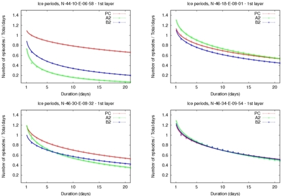
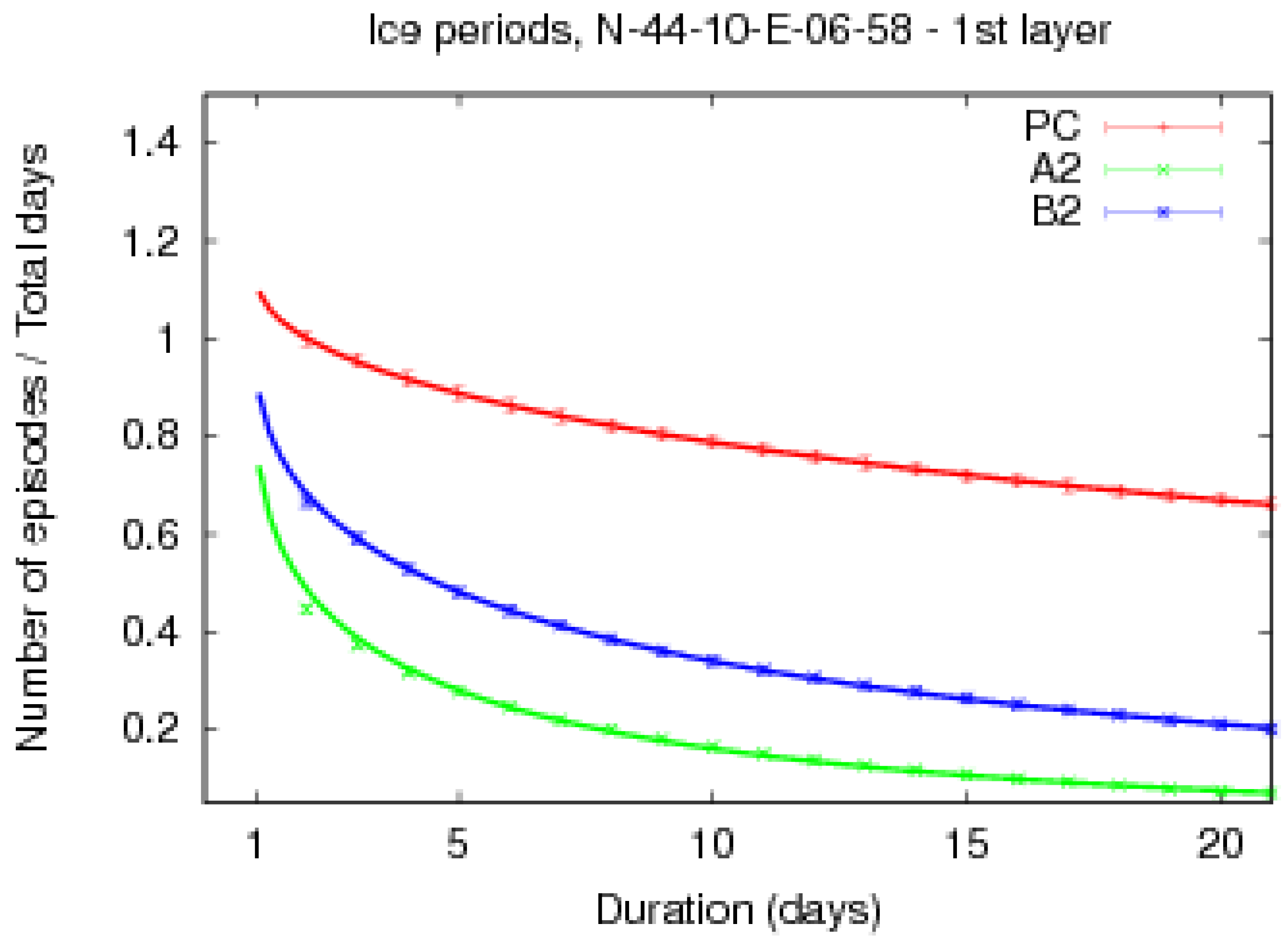
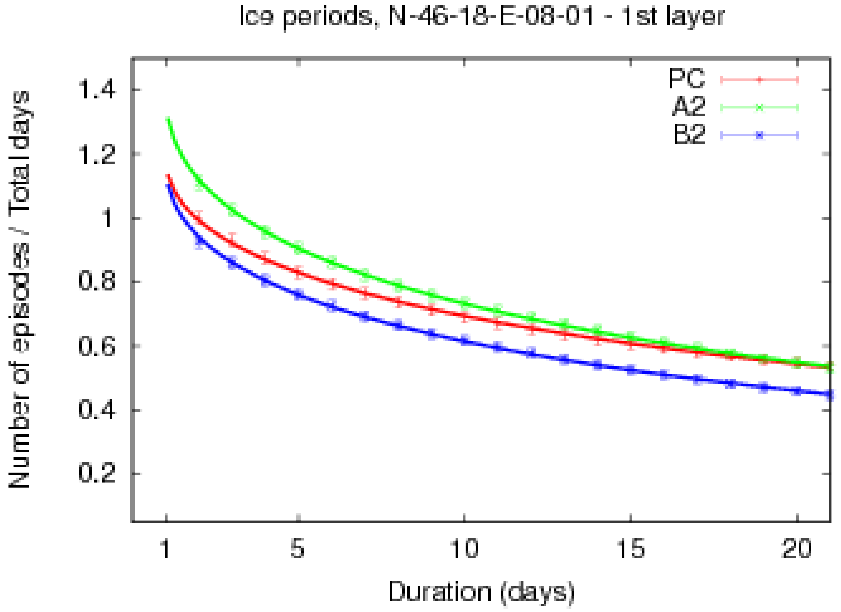
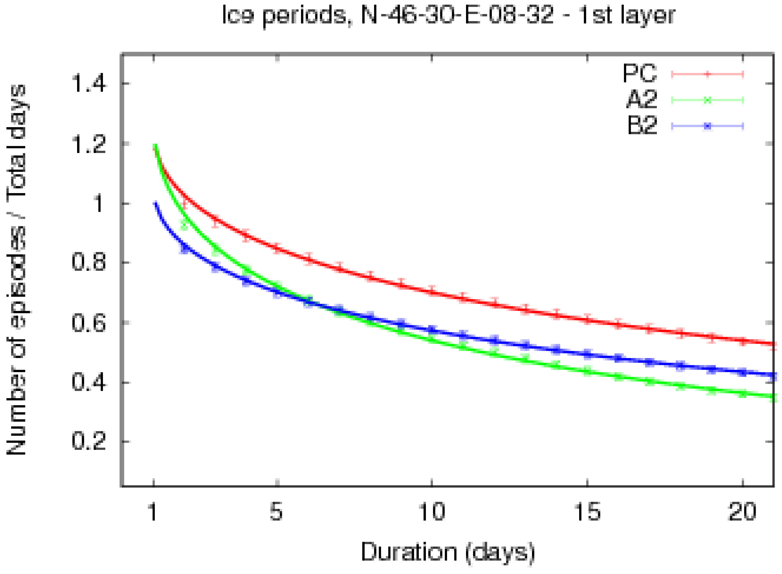
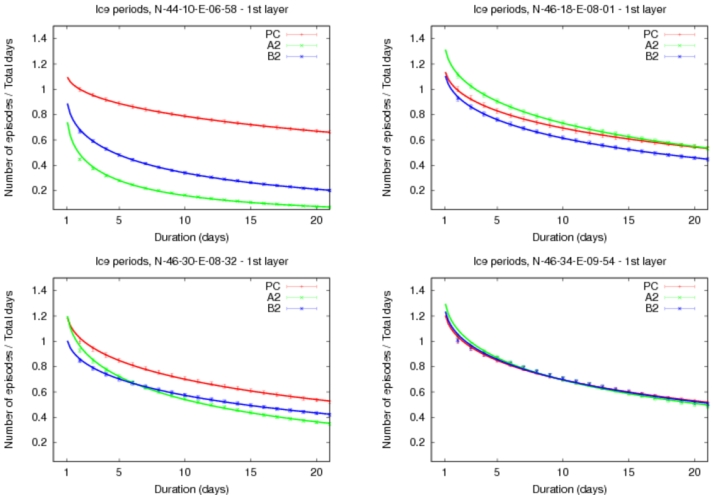
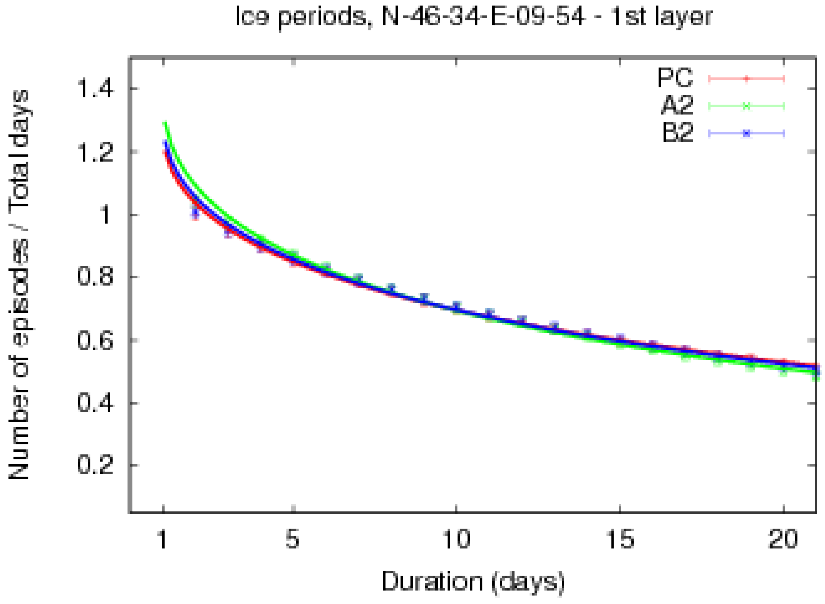
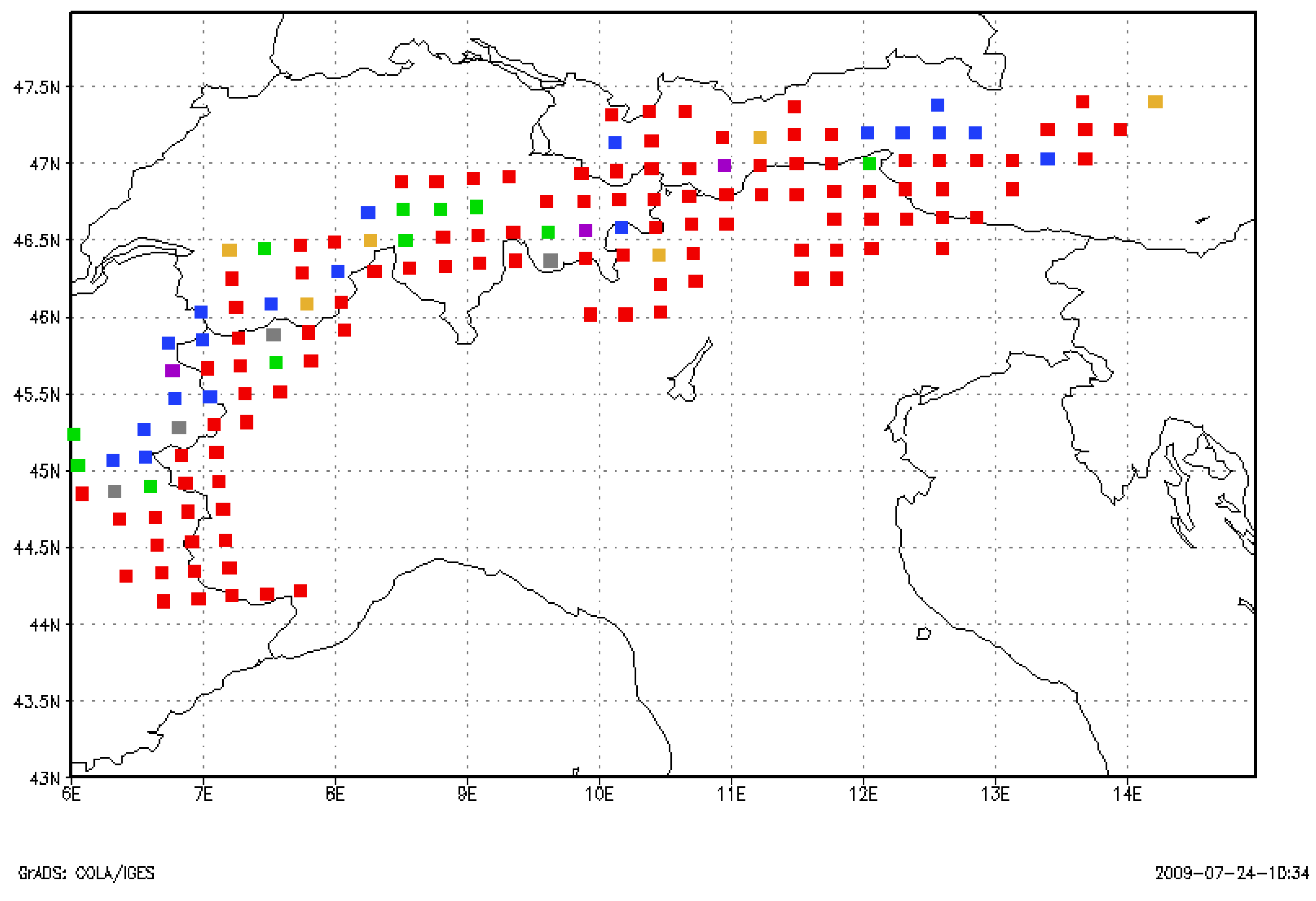
4.1. Categorisation of the Trends in Cold Breaks Frequency versus Their Length

Among the simulation points mentioned in Section 3, for those characterised by an orographic elevation higher than 1500 m above the sea level, plots like those reported in Figure 1, Figure 2, Figure 3 and Figure 4 were produced. These figures represent the frequencies of cold breaks of a given length versus their length. The frequencies were normalised by dividing the actual number of events of a given length by the number of events of one day duration in PC (the reason for this choice will be given in Section 4.2). The dots represent the actual number of recorded events, while the error bars represent the standard deviation of the recorded events according to Poissonian statistics. The error bars are small compared to the figure size, since they are about 2% relative to the data.
Figure 1. Frequency of cold spells versus their duration: the case expected by hypothesizing increasing average temperature.
Water 02 00363 g001
Figure 2. Frequency of cold spells versus their duration: the case in which the number of events increases in a future scenario.
Water 02 00363 g002
Figure 3. Frequency of cold spells versus their duration: the case in which A2 and B2 curves cross each other.
Water 02 00363 g003
Figure 4. Frequency of cold spells versus their duration: the case of no difference in the climate scenarios
Water 02 00363 g004
Simulated results for various points in the area of study reveal several plausible trends for the frequency versus duration graphics. Under the A2 and B2 scenarios, the frequencies of cold spells can decrease (Figure 1), increase in a future scenario (Figure 2 under A2 scenario), show differential increases for various durations under A2 and B2 scenarios (Figure 3), or indicate no noticeable change from the PC (Figure 4). A complete schematisation of all possible behaviours can be found in Table 1.
Table 1. Categorization of the set of qualitatively different behaviours of the frequency of cold breaks versus their length.
CategoryExample trend figureDescription
Red1Number of cold breaks decreasing in FC
Blue2Number of cold breaks increasing in FC
Green3Number of short breaks greater in A2 than B2, number of long breaks greater in B2 than A2
Violet4No difference between PC and FC
Yellow(not shown)No difference between PC and A2
Grey(not shown)No difference between PC and B2
If one considers the most obvious behaviour, i.e., that, as a consequence of the global warming, the increase in the average temperature will induce a decrease of the number of cold spells, it is expected that all, or at least the majority of the simulation points will fall into the red category in table 1. A more detailed analysis of the data shows that the actual situation is not as trivial as one could expect. Figure 5 shows, by using the colors as representative of the categories defined in table 1, the distribution of the categories for the frequency-length trend lines.
Figure 5. Geographical distribution of simulation points characterised by trend lines as described in Table 1 (that same table can also be referenced as a legend for the colors used in this figure).
Water 02 00363 g005
In particular, although about 70% of the simulation points belong to the red category, the remaining 30% do not. Moreover, an interesting spatialisation of this information is evident. There are two clusters of blue dots in Savoie (France) and in the Tauern (Austria). The presence of these clusters means that in those regions, no matter whatever scenario could become more realistic between A2 and B2, climate change will cause an increase of cold breaks in the future, for all of the possible lengths. One additional cluster in the Lepontine Alps belongs to the green category: according to its description in Table 1 and observing Figure 3, this means that a difference in the climate scenario will imply very large and not-simply-understandable differences in the cold breaks occurrence. For this category, in fact, the A2 scenario has a greater number of short cold breaks with respect to B2, while for long cold breaks, B2 has a greater number with respect to A2.
The evidence coming from these figures can be explained in other words. In 70% of the simulation points global warming will result in a shift of the temperature distribution towards higher temperatures, without altering too much the shape of the distribution. In the remaining 30% of the simulation points, not only will the mean temperature increase for both scenarios, but also the temperature distributions will be altered in such a way that the extremes may show even higher frequencies, even within the coldest part of the distribution tail.
Table 2. Number of simulation points in the Alps above and below 2000 m ASL for each category as defined in Table 1 (the total number of Alpine points is 145).
CategoryBelow 2000 m ASLAbove 2000 m ASL
Red6834
Blue910
Green65
Violet12
Yellow04
Grey33
Moreover, a distinct classification between points over and under 2000 m a.s.l., reported in Table 2, was conducted. Despite the fact that the total number of points below 2000 m a.s.l. (middle column in the table) is roughly half (58 cases versus 87) of those above 2000 m a.s.l. (right column), the only row of the table which halves (from 68 cases to 34) passing from the central to the right column is the one corresponding to the red color category. In conclusion, the response to the climate change will be more differentiated at higher altitudes, with consistent alterations of the temperature distributions in the FC, while, at lower altitudes, the global warming will mostly result in a shift in the temperature distribution towards warmer temperatures.

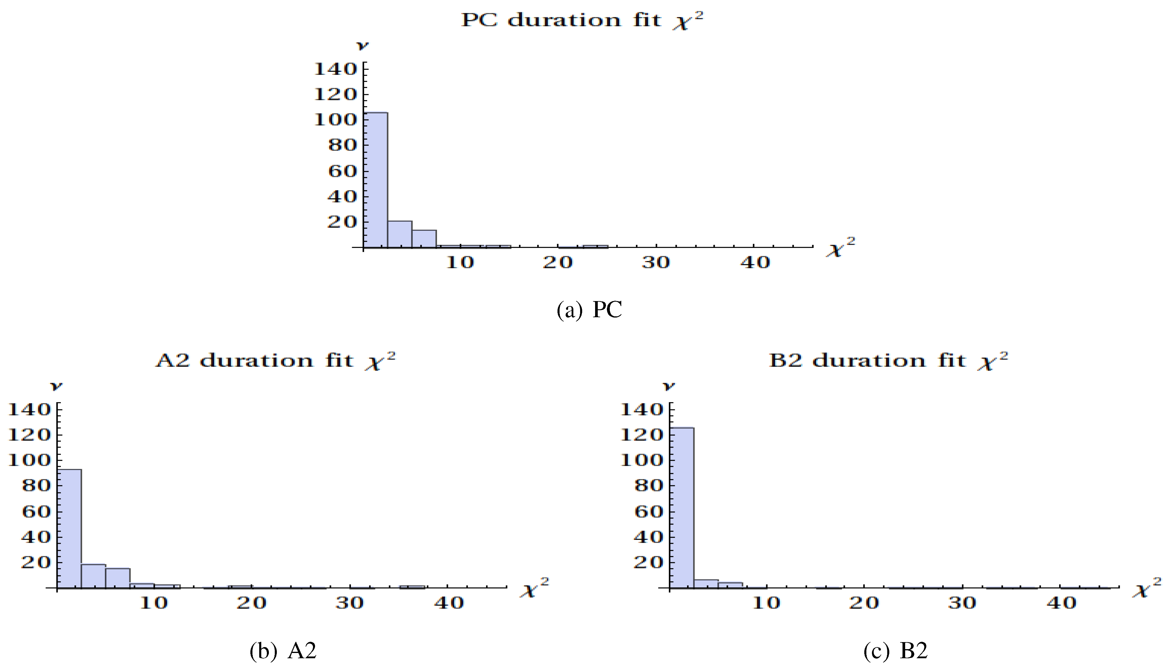
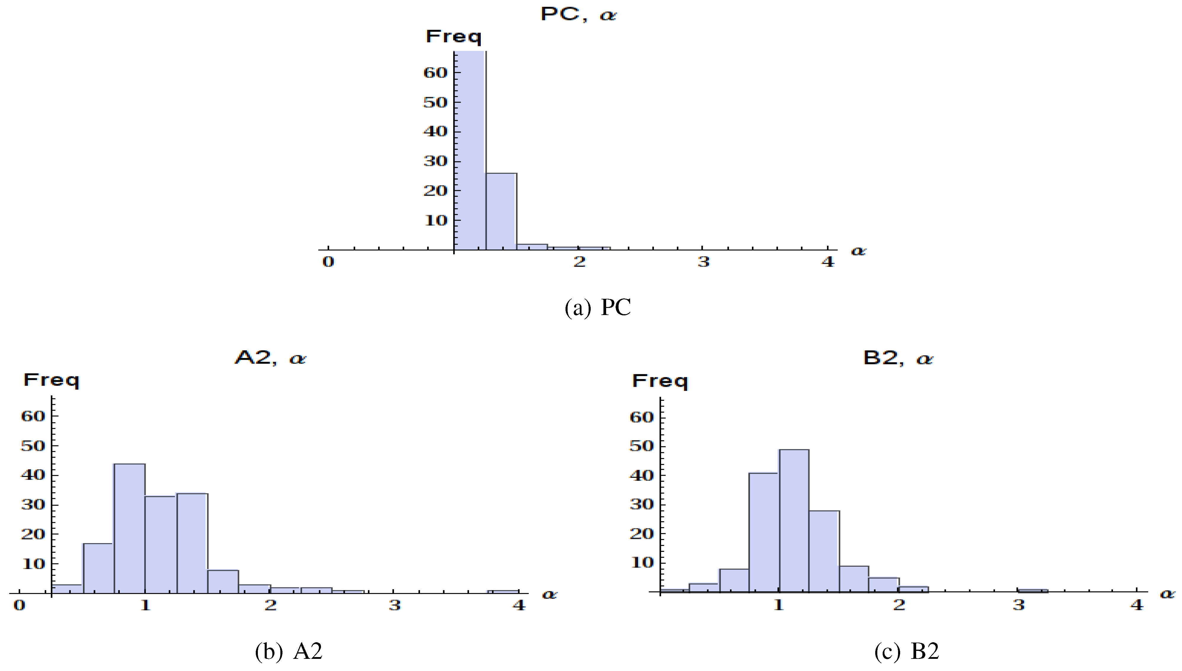
4.2. Global Statistics of the Occurrence of Cold Breaks
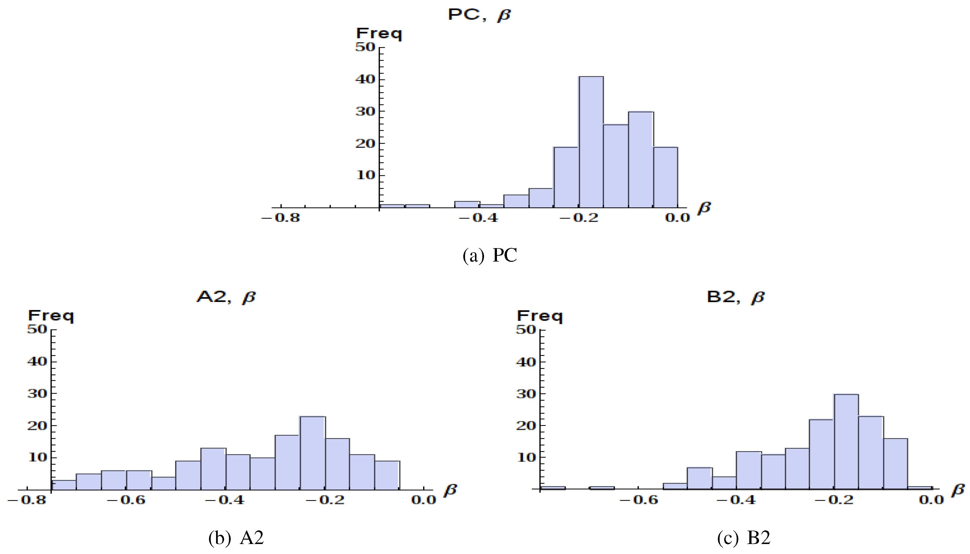
Besides the blue and green clusters illustrated in Figure 5, it is interesting to study the effects of climate change over the whole area on the occurrence and the length of cold breaks. To accomplish this task, it is necessary to compare somehow the plots of the frequency of cold breaks versus their length. In Section 4.1 it has been stated that frequency data were normalised in order that the frequency of 1-day-long events in PC was equal to 1. In this part of this study, the choice of this normalisation allows easier comparison of simulation points possessing different absolute frequencies of cold breaks, while the categorisation described in Section 4.1 is valid independently from the absolute frequencies. To characterise globally the occurrence of cold breaks, it is necessary to study how the number of cold breaks decays with increasing its length.
To reduce the information contained in each plot of Section 4.1 into more manageable values, it was decided to fit, for each scenario and simulation point, the dots of the plots sampled in Figure 1, Figure 2, Figure 3 and Figure 4 with a two parameters curve. Even if, for the moment, the physical meaning of these fits does not appear clear, however this method offers a tool to condense the information in these two parameters.
The best model to fit the data was found to be the following exponential law:
N = α e β L
where N is the normalized frequency of the cold breaks and L is their length, expressed in days. α and β are the free parameters of the fit, and can be related to a physical meaning. The higher α is, the higher the number of cold breaks is, so the lower is the average temperature. β, which is negative by definition, represents the decay of the number of events at the increasing of their length. Hence, the higher is | β | (in absolute value), the more rapid the decay is, and this can be related to more frequent temperature variations around 0 C .
The choice of the fitting model of Equation (1) has been made in order that the physical meaning of the free parameters was the one above explained. However, as it will be shown, Equation (1) is also a good model for fitting the data, and is statistically most adherent to the data distribution than other models, which were tested too, like the exponential tested in [52].
The panels of Figure 6 show the distribution of the calculated values of the χ 2 variables for the fits of each simulation point. Each of these plots show very low values of the χ 2 variables. Choosing a significance level a = 5 % , the lower and upper critical values of the χ 2 test, with 18 degrees of freedom, are χ inf 2 = 8 . 23 and χ sup 2 = 31 . 53 . As it can be seen from the Figures 6, almost all fits show χ 2 < χ sup 2 , meaning that Equation (1) actually fits the data quite well. For most of the simulation points, it is also true that χ 2 < χ inf 2 . This means that the Poissonian determination of the error bars gives standard deviations that are too large for the data, but it does not invalidate the fitting model itself, and hence the physical meaning of the fitting model parameters α and β, which are the main result for this stage of the analysis.
Figure 6. Distributions of the values of χ 2 variables calculated in the evaluation of the goodness of fit tests.
Water 02 00363 g006
Once having obtained the couple of values α and β for each simulation point and each climate scenario, it is possible to use them to gain some more general conclusions on the occurrence of cold breaks.
The histograms of Figure 7 and Figure 8 show the distributions of the obtained values for the fit parameters, respectively α and β. From Figure 7 it is possible to see that the distributions of FC differ in both spread and peak height. Recalling the meaning of the parameter α, it means that average temperature will vary differently in different places. The mode of the distribution for A2 scenario is shifted towards slightly lower values than for the peak of B2. This means that, on average, A2 scenario will be warmer and will show less cold breaks than B2. Also, the height of the A2 peak is lower, and its spread is larger than B2 situation. This means that the spatial effects of climate change will show greater variations in A2 with respect to B2.
Figure 7. Distributions of the values of the α parameter of Equation (1). All the histograms have been produced to represent the same number of samples, but the one of panel 8(a) has been cut to make easier a comparison with the other panels, using the same vertical scale; it shows a very high peak on α 1 (up to 120) due to the choice of data normalization (see Section 4.1).
Water 02 00363 g007
Considering Figure 8, relative to the fit parameter β, it is possible to notice that the peak of the distributions is more or less in the same position for PC and B2, while it is shifted to lower values in scenario A2. This means that, on average, the temperature variability is greater for the A2 scenario than in the others. Another difference that is evident is the spread of the three distributions. In PC, the majority of the data is located between the peak value and 0, while this is not true for FC. A2 scenario shows a greater spread of β towards the small values; PC and B2 have just some outliers, while A2 still has a distribution of data with no gaps, with higher values in the left tail.
In order to assess the statistical significance of these distributions and of their differences, the runs test (described in [53]) was performed. This test gives the probability that two samples of data belong to the same underlying probability density distribution. In particular, the distributions of the α and β
Figure 8. Distributions of the values of the β parameter of Equation (1).
Water 02 00363 g008
parameters for every climate scenario were compared ‘pair by pair’, and the results of these tests are shown in Table 3.
Table 3. Resume of results for the runs tests comparing the distributions of the fit α and β parameters
Pair of scenariosDistributionProbability
α parameter
PC - A2Different > 99 %
PC - B2Different > 99 %
A2 - B2Different > 99 %
β parameter
PC - A2Different > 99 %
PC - B2Same 20 %
A2 - B2Different 90 %
Basically, almost all dataset exhibit high probability (at least 90 % or even higher than 99 % ) to belong to different probability density distribution. Translated in physical words, this means that the occurrence of cold breaks is statistically significantly different for the different scenarios. This difference is much more evident in the analysis of the α parameter, which is related to the number of short length breaks and hence average temperature. The difference between the two future climate scenarios is less evident, but still statistically significant considering the β parameter (concerned with temperature time variability one), at least when comparing the A2 scenario with the other two, where, in both cases, A2 is the most variable. The difference in the β parameter histograms of PC and B2 is not statistically significant, since these two data sets have 20 % probability of belonging to the same probability distribution. Hence, the temporal temperature variability is not deemed to be statistically different in PC and B2.

5. Conclusions

The investigation presented in this paper aims to further the understanding of the occurrence of cold spells on the Alps in the future climate. Two 30-year periods (2071-2100) belonging to two scenarios A2 and B2 were compared with a 30-year period belonging to the present climate (1961-1990). The result of this analysis showed that some behaviours appear not to be trivial. In fact, at a first approximation, it could be foreseen that the increment of temperature associated with global warming could force the number of cold breaks to decrease, at least on average, during the FC. On the contrary, this study reveals that, in the Alpine area, there are some zones (which on average constitutes 30% of the total area) in which this is not predicted to occur, even if, in general, the results of [2] are confirmed.
Evidently, the temperature distribution in those zones will not just simply shift towards warmer temperature, thus reducing the number of cold spells alone, but will also modify its shape, leading to an increase in the probability of cold spells in some occasions.
Another important result was obtained by carrying out global tests on the occurrence of cold breaks. These show that variability in the occurrence of cold breaks is strongly affected by climate change. This confirms, a posteriori, that in the Alpine area the temperature variability is also expected to increase. In addition to this already important result, a model relating the number of cold breaks to their duration has been found. This model has been used as a tool to describe the variation in the occurrence of cold breaks related to climate change, and was seen to be a very good model. A better interpretation of this model could be a starting point for future work.
The new results obtained in this context, as well as the advances in the climate modelling, will hopefully help to tune the knowledge of the scientific community with regard to changes in the occurrence of extreme events.

Acknowledgements

The authors thank the Earth System Physics Section of the ICTP, Italy, for having provided the RegCM3 dataset. S. Oh is grateful to the University of Torino (UT) for having supported her visit to the Department of General Physics of UT under the World Wide Style grant. C. Cassardo and S. K. Park are supported by the government of Italy and Korea, respectively, for visiting each institution for collaborative research via the bilateral scientific agreements. This work is partly supported by the Ministry of Environment, Korea, under the National Comprehensive Measures against Climate Change Program (No. 1700-1737-322-210-13), and by the Ministry of Education, Science and Technology, Korea, through the National Research Foundation grant (No. 2009-0083527). All authors are thankful to A. Tata, the S & T Attaché of the Italian Embassy in Korea, for his help in organising two Korea-Italy Joint Seminars on Climate Change, in which some preliminary results of this study have been presented. A special mention has to be dedicated to V. Bright, who helped in proofreading the manuscript.

References

  1. Stull, R.B. An Introduction to Boundary Layer Meteorology; Springer: Dordrecht, the Netherlands, 1988. [Google Scholar]
  2. Solomon, S.; Quin, D.; Manning, M.; Chen, Z.; Marquis, M.; Averyt, K.B.; Tignor, M.; Miller, H.L. Climate Change 2007: The Physical Science Basis; Cambridge University Press: Cambridge, UK, 2007. [Google Scholar]
  3. Shabbar, A.; Bonsal, B. An Assessment of Changes in Winter Cold and Warm Spells over Canada. Natural Hazards 2002, 29, 173–188. [Google Scholar] [CrossRef]
  4. Nakicenovic, N.; Swart, R. Special Report on Emissions Scenarios: A Special Report of Working Group III of the Intergovernmental Panel on Climate Change; Cambridge University Press: Cambridge, UK, 2001. [Google Scholar]
  5. Kharin, V.V.; Zwiers, F.W. Changes in the extremes in an ensamble of transient climate simulations with a coupled atmosphere-ocean GCM. J. Clim. 2000, 13, 3760–3788. [Google Scholar] [CrossRef]
  6. Dickinson, R.E.; Errico, R.M.; Giorgi, F.; Bates, G.T. A regional climate model for the western United States. Climatic Change 1989, 15, 383–442. [Google Scholar] [CrossRef]
  7. Giorgi, F. Simulation of regional climate using a limited area model nested in a general circulation model. Journal of Climate 1990, 3, 941–963. [Google Scholar] [CrossRef]
  8. Halenka, T.; Kalvova, J.; Chladova, Z.; Demetrova, A.; Zemankova, K.; Belda, M. On the capability of RegCM to capture extremes in long term regional climate simulation-comparison with the observations for Czech Republic. Theor. Appl. Climatol. 2006, 86, 121–142. [Google Scholar] [CrossRef]
  9. Im, E.S.; Kwon, W.T. Characteristics of Extreme Climate Sequences over Korea Using a Regional Climate Change Scenario. Sci. Online Lett. Atmos. 2007, 3, 17–20. [Google Scholar]
  10. Robertson, A.W.; Kirshner, S.; Smyth, P. Downscaling of daily rainfall occurrence over Northeast Brazil using a Hidden Markov model. J. Meteor. Soc. Japan. 2004, 82, 4407–4424. [Google Scholar] [CrossRef]
  11. Schär, C.; Vidale, P.L.; Lüthi, D.; Frei, C.; Häberli, C.; Liniger, M.; Appenzeller, C. The role of increasing temperature variability in European summer heat waves. Nature 2004, 432, 427–332. [Google Scholar]
  12. Beniston, M. Mountain weather and climate: A general overview and a focus on climatic change in the Alps. Hydrobiologia 2006, 562, 3–16. [Google Scholar] [CrossRef]
  13. Regional Climate Change and Adaptation - The Alps Facing the Challenge of Changing Water Resources; European Environment Agency: Copenaghen, Denmark, 2009.
  14. Beniston, M.; Goyette, S. Changes in variability and persistance of climate in Switzerland: Exploring 20th century observations and 21st century simulations. Global and Planetary Change 2007, 57, 1–15. [Google Scholar] [CrossRef]
  15. Giorgi, F.; Bi, X.; Pal, J.S. Mean, interannual variability and trends in a regional climate change experiment over Europe. I. Present-day climate (1961–1990). Clim. Dynam. 2004, 23, 839–858. [Google Scholar] [CrossRef]
  16. Giorgi, F.; Bi, X.; Pal, J.S. Mean, interannual variability and trends in a regional climate change experiment over Europe. II: climate change scenarios (2071–2100). Clim. Dynam. 2004, 23, 839–858. [Google Scholar] [CrossRef]
  17. Gao, X.J.; Pal, J.S.; Giorgi, F. Projected changes in mean and extreme precipitation over the Mediterranean region from a high resolution double nested RCM simulation. Geophys. Res. Lett. 2006, 33, 1–4. [Google Scholar] [CrossRef]
  18. Grell, G.A.; Dudhia, J.; Stauffer, D. A description of the Fifth-Generation Penn State/NCAR Mesoscale Model (MM5); NCAR: Boulder, CO, USA, 1994. [Google Scholar]
  19. Pal, J.; Small, E.; Eltahir, E. Simulation of regional-scale water and energy budgets: representation of subgrid cloud and precipitation processes within RegCM. J. Geophys. Res. 2000, 105, 29579–29594. [Google Scholar] [CrossRef]
  20. Anthes, R. A cumulus parametrization scheme utilizing a one-dimensional cloud model. Mon. Wea. Rev. 1977, 105, 270–286. [Google Scholar] [CrossRef]
  21. Giorgi, F. Sensitivity of simulated summertime precipitation over the western United States to different physics parametrization. Mon. Wea. Rev. 1991, 119, 2870–2888. [Google Scholar] [CrossRef]
  22. Emanuel, K.A. A scheme for representing cumulus convection in large-scale models. J. Atmos. Sci. 1991, 48, 2313–2329. [Google Scholar] [CrossRef]
  23. Grell, G. Prognostic evaluation of assumptions used by cumulus parametrizations. Mon. Wea. Rev. 1993, 121, 764,787. [Google Scholar] [CrossRef]
  24. Emanuel, K.A.; Živković-Rothman, M. Development and evaluation of a convection scheme for use in climate models. J. Atmos. Sci. 1999, 56, 1766–1782. [Google Scholar] [CrossRef]
  25. Dickinson, R.; Henderson-Sellers, A.; Kennedy, P. Biosphere-Atmosphere Transter Scheme (BATS) Version 1e as Coupled to the NCAR Community Climate Model; NCAR: Boulder, CO, USA, 1993. [Google Scholar]
  26. Giorgi, F.; Francisco, R.; Pal, J.S. Effects of a subgrid-scale topography and land use scheme on the simulation of surface climate and hydrology. Part I : Effects of temperature and water vapour disaggregation. J. Hydrometeor. 2003, 4, 317–333. [Google Scholar] [CrossRef]
  27. Elguindi, N.; Bi, X.; Giorgi, F.; Nagarajan, B.; Pal, J.; Solmon, F.; Rauscher, S.; Zakey, A. RegCM version 3.1 User’s Guide; ICTP: Trieste, Italy, 2007. [Google Scholar]
  28. Giorgi, F.; Bates, G.T.; Nieman, S.J. The multi-year surface climatology of a regional atmospheric model over the western United States. J. Clim. 1993, 6, 75–95. [Google Scholar] [CrossRef]
  29. Giorgi, F.; Shields, C. Tests of precipitation parametrizations available in latest version of NCAR regional climate model (RegCM) over continental United States. J. Geophys. Res. 1999, 104, 6353–6375. [Google Scholar] [CrossRef]
  30. Diffenbaugh, N.S.; Pal, J.S.; Trapp, R.J.; Giorgi, F. Fine-scale processes regulate the response of extreme events to global climate change. PNAS 2005, 102, 15774–15778. [Google Scholar] [CrossRef] [PubMed]
  31. Solomon, F.; Giorgi, F.; Liousse, C. Aerosol modelling for regional climate studies: application to anthropogenic particles and evaluation over a European/African domain. Tellus B 2006, 58, 51–72. [Google Scholar] [CrossRef]
  32. Pal, J.S.; Elthair, A.B. Teleconnections of soil moisture and rainfall during the 1993 Midwest summer flood. Geophys. Res. Lett. 2002, 29, 1865. [Google Scholar] [CrossRef]
  33. Pal, J.S.; Giorgi, F.; Bi, X. Consistency of recent European summer precipitation trends and extremes with future regional climate projections. Geophys. Res. Lett. 2004, 31, L13202. [Google Scholar] [CrossRef]
  34. White, M.; Diffenbaugh, N.; Jones, G.; Pal, J.S.; Giorgi, F. Increased heat stress in the 21st century reduces and shifts premium wine production in the United States. PNAS 2006, 103, 11271–11222. [Google Scholar] [CrossRef] [PubMed]
  35. Abiodun, B.J.; Pal, J.S.; Afiesimama, E.A.; Gutowski, W.J.; Adedoyin, A. Simulation of West African Monsoon using RegCM3. Part II: Impact of desertification and deforestation. Theor. Appl. Climatol. 2007, 93, 245–261. [Google Scholar] [CrossRef]
  36. Pal, J.S.; Elthair, A.B. A feedback mechanism between soil moisture distribution and storm tracks. Quart. J. Roy. Meteor. Soc. 2003, 129, 2279–2297. [Google Scholar] [CrossRef]
  37. Cassardo, C.; Ji, J.J.; Longhetto, A. A study of the performances of a Land Surface Process Model (LSPM). Bound. Layer Meteor. 1995, 72(1-2), 87–121. [Google Scholar] [CrossRef]
  38. Cassardo, C. The Land Surface Process Model (LSPM) Version 2006; Dipartimento di Fisica Generale Amedeo Avogadro: Torino, Italy, 2006. [Google Scholar]
  39. Ruti, P.M.; Cassardo, C.; Cacciamani, C.; Paccagnella, T.; Longhetto, A.; Bargagli, A. Intercomparison between BATS and LSPM surface schemes, using point mocrometeorological data set. Contrib. Atmos. Phys. 1997, 70, 201–220. [Google Scholar]
  40. Cassardo, C.; Carena, E.; Longhetto, A. Validation and sensitivity tests on improved parametrizations of a Land Surface Process Model (LSPM) in the Po Valley. Il Nuovo Cimento 1998, 21, 189–213. [Google Scholar]
  41. Cassardo, C.; Loglisci, N.; Romani, M. Preliminary results of an attempt to provide soil moisture datasets in order to verify numerical weather prediction models. Il Nuovo Cimento 2005, 28, 159–171. [Google Scholar]
  42. Cassardo, C.; Loglisci, N.; Gandini, D.; Qian, M.W.; Niu, Y.P.; Ramieri, P.; Pelosini, R.; Longhetto, A. The flood of November 1994 in Piedmont, Italy: a quantitative simulation. Hydrol. Process. 2002, 16, 1275–1299. [Google Scholar] [CrossRef]
  43. Cassardo, C.; Loglisci, N.; Paesano, G.; Rabuffetti, D.; Qian, M.W. The hydrological balance of the October 2000 flood in Piedmont, Italy: quantitative analysis and simulation. Physical Geography 2006, 27, 411–434. [Google Scholar] [CrossRef]
  44. Cassardo, C.; Mercalli, L.; Cat Berro, D. Charateristics of the summer 2003 heat wave in Piedmont, Italy, and its effects on water resources. J. Korean Meteorol. Soc. 2007, 43, 195–1221. [Google Scholar]
  45. Feng, J.; Liu, X.; Cassardo, C.; Longhetto, A. A model of plant transpiration and stomatal regulation under the condition of waterstress. J. Desert Res. 1997, 17, 59–66. [Google Scholar]
  46. Loglisci, N.; Qian, M.W.; Cassardo, C.; Longhetto, A.; Giraud, C. Energy and water balance at soil-air interface in a Sahelian region. Adv. Atmos. Sci. 2001, 18, 897–909. [Google Scholar]
  47. Cassardo, C.; Park, S.K.; Thakuri, B.M.; Priolo, D.; Zhang, Y. Soil Surface Energy and Water Budgets during a Monsoon Season in Korea. J. Hydrometeor. 2009, 10, 1379–1396. [Google Scholar] [CrossRef]
  48. Zhang, Y.; Cassardo, C.; Ye, C.; Galli, M. A Landfall Typhoon Simulation in a Coupled Land Surface Process Model Wirh WRF. Asia-Pacific J. Atmos. Sci. 2010, in press. [Google Scholar]
  49. Burden, R.L.; Faires, J.D. Numerical Analysis; Brooks Cole: Pacific Grove, CA, USA, 2004. [Google Scholar]
  50. Masson, V.; Champeaux, J.L.; Chauvin, F.; Meriguet, C.; Lacaze, R. A global database of land surface parameters at 1 km resolution in meteorological and climate models. J. Clim. 2003, 16, 1261–1282. [Google Scholar] [CrossRef]
  51. Bonanno, R.; Loglisci, N.; Cavalletto, S.; Cassardo, C. Soil freezing in LSPM SVAT scheme. Water 2010. submitted. [Google Scholar]
  52. Wilks, D.S. Statistical Methods in Atmospheric Sciences; Academic Press: Oxford, UK, 1995. [Google Scholar]
  53. Wald, A.; Wolfowitz, J. On a test wether two samples are from the same population. Ann. Math Statist. 1940, 11, 147–162. [Google Scholar] [CrossRef]

