An Experimental Study on the Influence of Rigid Submerged Vegetation on Flow Characteristics in a Strongly Curved Channel

Abstract

Flow dynamics in strongly curved channels with submerged vegetation play a crucial role in riverine ecological processes and morphodynamics, yet the combined effects of sharp curvature and rigid submerged vegetation remain inadequately understood. This study presents a comprehensive experimental investigation into the influence of rigid submerged vegetation on the flow characteristics within a 180° strongly curved channel. Laboratory experiments were conducted in a U-shaped flume with varying vegetation configurations (fully vegetated, convex bank only, and concave bank only) and two vegetation heights (5 cm and 10 cm). The density of vegetation ϕ was 2.235%. All experimental configurations exhibited fully turbulent flow conditions (R_e > 60,000) and subcritical flow regimes (F_r < 1), ensuring gravitational dominance and absence of jet flow phenomena. An acoustic Doppler velocimeter (ADV) was employed to capture high-frequency, three-dimensional velocity data across five characteristic cross-sections (0°, 45°, 90°, 135°, 180°). Detailed analyses were performed on the longitudinal and transverse velocity distributions, cross-stream circulation, turbulent kinetic energy (TKE), power spectral density, turbulent bursting, and Reynolds stresses. The results demonstrate that submerged vegetation fundamentally alters the flow structure by increasing flow resistance, modifying the velocity inflection points, and reshaping turbulence characteristics. Vegetation height was found to delay the manifestation of curvature-induced effects, with taller vegetation shifting the maximum longitudinal velocity to the vegetation canopy top further downstream compared to shorter vegetation. The presence and distribution of vegetation significantly impacted secondary flow patterns, altering the direction of cross-stream circulation in fully vegetated regions. TKE peaked near the vegetation canopy, and its vertical distribution was strongly influenced by the bend, causing the maximum TKE to descend to the mid-canopy level. Spectral analysis revealed an altered energy cascade in vegetated regions and interfaces, with a steeper dissipation rate. Turbulent bursting events showed a more balanced contribution among quadrants with higher vegetation density. Furthermore, Reynolds stress analysis highlighted intensified momentum transport at the vegetation–non-vegetation interface, which was further amplified by the channel curvature, particularly when vegetation was located on the concave bank. These findings provide valuable insights into the complex hydrodynamics of vegetated meandering channels, contributing to improved river management, ecological restoration strategies, and predictive modeling.

1. Introduction

Flow dynamics in open-channel bends are crucial due to their significant impact on alluvial and ecological processes. These flows exhibit complex helical patterns that induce cross-stream flows near the bed, leading to the redistribution of streamwise momentum within the channel cross-section [1,2,3]. This phenomenon has been explored through various approaches such as theoretical derivation, field observations, physical model experiments, and numerical simulations.

For example, Rüther and Olsen [4] proposed a k-ε turbulence model tailored for simulating secondary flow in a 90° narrow flume, demonstrating that the orientation of secondary flow is governed by the direction of shear stress in the near-bed zone. Through laboratory experimental investigations, Zeng et al. [5] illustrated that turbulent kinetic energy (TKE) within channel bends is substantially higher compared to that at the inlet and outlet sections. Roca et al. [6] reported observational evidence indicating that maximum vorticity intensifies along curved channels, increasing progressively from the bend entrance and peaking at cross-sections between 40° and 60° of the bend curvature. Blanckaert [7] and Blanckaert and De Vriend [8] identified water surface gradient and streamwise curvature variations as the primary drivers of velocity redistribution in sharp-bend channels. Vaghefi et al. [9] observed two persistent clockwise vortices in the cross-sectional streamlines of curved channels, noting that the maximum shear stress arises in the region from the bend entrance to the apex, particularly adjacent to the inner wall. Shaheed et al. [10] employed a 3D OpenFOAM numerical model to examine the impact of secondary currents on velocity distributions in channel bends, with their findings highlighting the superior performance of the standard k-ε model. Bai et al. [3] emphasized that the interaction between the main flow and secondary flow persists throughout the entire length of curved channels. In a numerical study by Yan et al. [11], a high unit discharge core was found to form near the inner bend due to the potential-vortex effect, which gradually migrated toward the outer bend under the influence of secondary circulation.

Even so, these studies only focus on flow features over curved channels; conditions more consistent with aquatic vegetation have received less attention and are not well understood, especially with regard to submerged vegetation. For natural rivers, the presence of aquatic vegetation exerts dual influences: it not only regulates biological dynamics within the aquatic ecosystem but also modifies key hydrodynamic processes. Specifically, such vegetation can mitigate flow velocity, elevate water levels, and reduce a river’s flood-carrying capacity [12]. In particular, three zones are examined for flows with submerged vegetation; these are lower vegetation, upper vegetation, and non-vegetated zones [13]. Therefore, gaining insights into the hydrodynamic–vegetation interactions holds significant implications for the sustainable management of water resources and the ecological conservation of aquatic environments [14].

In recent years, plenty of studies have focused on the water flow motions within rigid and submerged vegetation. For example, Lopez & Garcia [15] numerically analyzed the mean flow and turbulence structure in open channels with rigid, nonemergent vegetation and found that the maximum turbulent intensity in vertical and transverse directions appears in the canopy of the vegetation. Ghisalberti & Nepf [16] pointed out that all vertical profiles of mean velocity contained an inflection point, which makes the flow susceptible to Kelvin–Helmholtz instability. Carollo et al. [17] experimentally studied the flow over flexible bottom vegetation using a two-dimensional acoustic Doppler velocimeter and found that the measured velocity distributions are S-shaped and exhibit a three-zone profile. Ohmoto et al. [18] experimentally found that the secondary currents with the submerged vegetation zone installed at one side of a channel became stronger when compared with the secondary currents with the submerged vegetation zone installed at the center of a channel. Nezu & Sanjou [19] investigated turbulence structures and coherent large-scale eddies in the vegetated canopy open-channel flows on the basis of LDA and PIV measurements as well as LES calculations. The results show that the mean velocity profile has an inflection point near the vegetation edge, and the ejections and sweeps govern turbulence structure and coherent motions in aquatic canopy flows. Liu et al. [20] numerically showed that the sign of the secondary flow parameter is determined by the rotational direction of secondary current cells, and its value is dependent on the flow depth. Devi & Kunar [21] carried out the experiment in an alluvial channel covered partially with submerged vegetation and indicated that the presence of vegetation reduces the velocity, Reynolds stress, and turbulent intensities in the downstream-vegetated region. Liu et al. [22] numerically studied the flow around submerged canopy patches with finite sizes and found that the streamwise bleeding flow decreased while the lateral and vertical bleeding flow increased as the array became denser. The large-eddy simulation (LES) model has been introduced to reproduce the production, propagation, and dissipation of K–H vortices at the top of the submerged vegetation to overcome the difficulties in modeling time-dependent turbulence [23,24,25,26].

These studies provide crucial insights into the effects of vegetation on water flow. However, the specific flow patterns in curved channels with vegetation are less understood and have received limited attention. The study of turbulent flow fields in curved and vegetated channels is complex due to the interaction between the channel’s meander and the obstruction caused by vegetation. The intricate flow patterns are influenced by these combined factors, leading to unique hydrodynamic characteristics [27]. Gorrick and Rodríguez [28] showed that the bank vegetation can reduce centrifugal effects at the bend entrance but enhance them at the bend exit over a mildly curved channel. Shan et al. [29] presented an analytical model for estimating the stage–discharge relationship in a meandering compound channel with submerged vegetation under high-flow conditions. Termini [30] indicated that the core of high velocity is always found away from the outer bank in the presence of vegetation. Wang et al. [27] numerically found that an increase in curvature ratios moves the main circulation cell towards the outer bank, while decreasing the drag coefficients streamwise and spanwise. Yang et al. [31] pointed out that the peak frequency determined from the spectrum at the vegetation and non-vegetation interface along a curved channel is still associated with the Kelvin–Helmholtz (K-H) instability.

However, limited research has addressed the impacts of rigid submerged vegetation configurations on the flow hydrodynamics of strongly curved channels. While existing studies have shed light on the complex flow dynamics in vegetated curved channels, they leave a critical research gap regarding how the specific configurations of rigid submerged vegetation modulate the hydrodynamic characteristics of strongly curved flows, such as how vegetation height alters the onset location of curvature effects, and how vegetation placement might change the Reynolds stress sign. This represents a key direction for future investigations, as elucidating these interactions is instrumental in optimizing water resource management and refining ecological protection strategies. Advancing knowledge in this domain will further facilitate the sustainable management of water resources and reinforce the ecological conservation of riverine ecosystems.

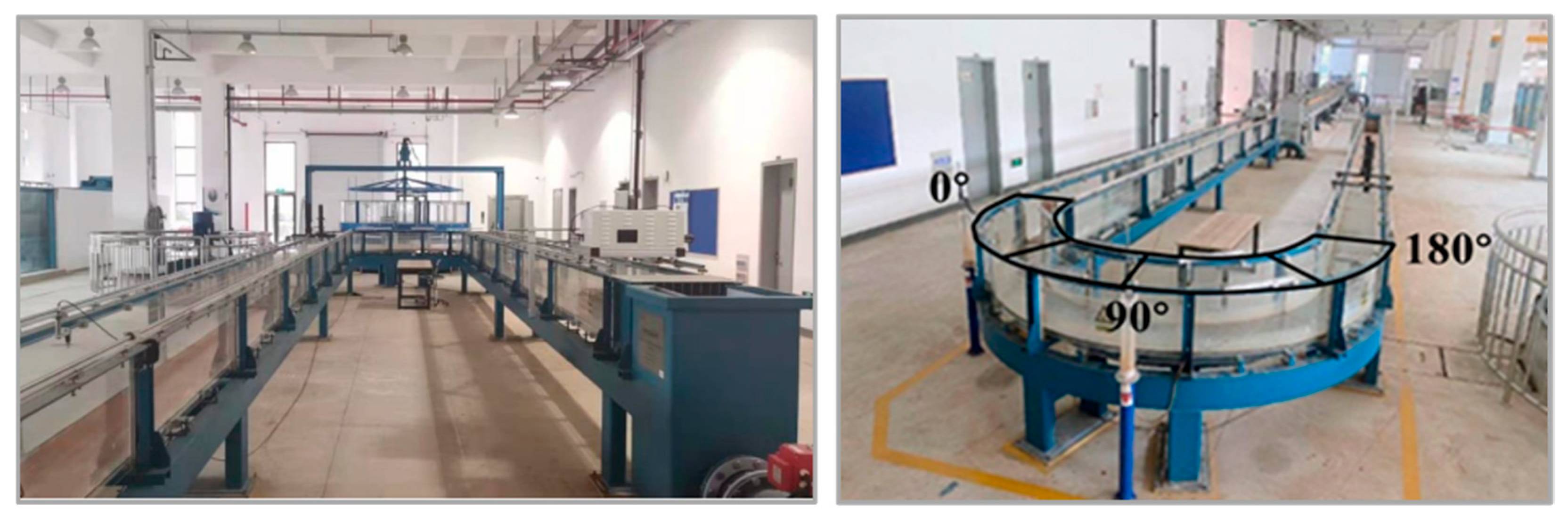
In this study, laboratory experiments were performed to examine the flow field in a 180° strongly curved channel under varied flow regimes and configurations of artificial rigid submerged vegetation. An acoustic Doppler velocimeter (ADV) was employed to acquire instantaneous three-dimensional (3D) flow velocities within the curved channel. The collected dataset was analyzed to characterize the hydrodynamic properties of flow in the presence of rigid submerged vegetation in such strongly curved channels. This paper is structured as follows: Section 2 presents a detailed account of the experimental setup and the various vegetation configurations adopted in the study. In Section 3, longitudinal and transverse velocity distributions, cross-sectional circulation patterns, turbulent kinetic energy (TKE), power spectral density (PSD), turbulent bursting events, and Reynolds stress components were computed for each experimental condition. These analyses aim to quantify the combined effects of channel curvature and vegetation on flow hydrodynamics. Finally, Section 4 summarizes the key findings of this research.

2. Experimental Setup

2.1. Flume Configuration and Hydraulic Parameters

The experiment was conducted in a U-shaped recirculating glass flume located in Zhoushan Campus of Zhejiang University. The flume, which is 33 m long, 0.4 m wide, and 0.4 m deep with a constant slope of 0.5% (Figure 1), consists of a 12 m long straight inflow reach, a 16 m long straight outflow reach, and a 180-degree curved reach with the radius of curvature R in the center position of the channel equal to 1.4 m. During the experiment, the flow rate was controlled in real time by a computer feedback control system, and the water level of the tail gate was kept constant. In this study, the flow rate $Q$ was set as 0.03 m³/s, and the water level at the downstream end was set to 0.35 m by an adjustable tailgate. A series of honeycomb grids was installed at the entrance of the channel to stabilize the flow and ensure that the water achieved a stable balance before entering the curved channel. The measurement process was started 30 min after the water tank equipment began to operate to ensure that the flow reached a stable state.

The flow regime was characterized using two fundamental dimensionless parameters that govern open channel flow dynamics: the Reynolds number ($R_e$), which represents the ratio of inertial to viscous forces and determines the transition from laminar to turbulent flow, and the Froude number ($F_r$), which indicates the relative importance of inertial to gravitational forces and distinguishes between subcritical and supercritical flow regimes [4]. The Reynolds number ($R_e$) is mathematically expressed as

$$R_e=(4U_{mo}{R}_h)/\nu ,$$

(1)

where $U_{mo}$ represents the bulk average velocity at the 0° cross-section (m/s), providing a characteristic velocity scale for the flow. The parameter $R_h$ denotes the hydraulic radius (m), calculated using the relationship $R_h=(Bh)/(B+2h)$, where $B$ is the channel width (m) and $h$ is the average flow depth at the 0° section (m). This formulation accounts for the wetted perimeter effects on flow resistance. The symbol $\nu$ = 1 × 10⁻⁶ m²/s represents the kinematic viscosity of water at laboratory conditions, characterizing the fluid resistance to deformation [6].

The Froude number ($F_r$) is defined by the following expression:

$$F_r=U_{mo}/\sqrt{g{h}_0},$$

(2)

where $g$ = 9.81 m/s² is the gravitational acceleration. The denominator $\sqrt{g{h}_0}$ represents the celerity of gravity waves in shallow water, making the Froude number a crucial parameter for characterizing free surface behavior and energy dissipation mechanisms. All experimental configurations exhibited fully turbulent flow conditions ($R_e$ > 60,000) and subcritical flow regimes ($F_r$ < 1), ensuring gravitational dominance and the absence of jet flow phenomena [20].

2.2. Vegetation Modeling and Configuration

Rigid wooden rods with a diameter $d$ of 6 mm and a height $H_v$ of 5 cm or 10 cm were used to mimic rigid submerged vegetation. In order to conform to natural vegetation density, the density of wooden rods $\varphi$ was set as 2.235%, which is expressed as the fraction of the volume of space occupied by the wooden rods [29]. The density is given as follows:

$$\varphi ={\displaystyle \frac{1}{4}}\pi ad,$$

(3)

where $a$ is the frontal area of the cylinders per unit volume.

The vegetation elements were arranged in a regular staggered pattern with specific geometric parameters. The longitudinal spacing $L_x$ = 0.05 m represents the center-to-center distance between vegetation elements along the flow direction, while the transverse spacing $L_y$ = 0.025 m denotes the distance between vegetation rows perpendicular to the flow. These spacing parameters directly influence the wake interactions and turbulence generation mechanisms. Four distinct vegetation configurations were implemented to systematically investigate spatial distribution effects (Figure 2). The bare case configuration served as an unvegetated reference baseline for comparative analysis, establishing the fundamental curvature-induced flow patterns without vegetation interference. The full case configuration featured complete vegetation coverage throughout the curved section with vegetation band width $B_v$ = 0.4 m equal to the full channel width, where $B_v$ is defined as the transverse width of the vegetated region measured from the channel bank. This configuration represents the maximum vegetation impact scenario.

The convex case configuration incorporated vegetation distributed exclusively along the inner convex bank with a vegetation band width $B_v$ = 0.2 m, representing half the channel width. This arrangement allowed us to investigate vegetation’s effects on the traditionally lower-velocity region of the bend. Conversely, the concave case configuration contained vegetation confined to the outer concave bank region with an identical vegetation band width $B_v$ = 0.2 m covering the remaining half channel width, enabling the study of vegetation’s impacts on the high-velocity outer-bank region, where centrifugal forces typically dominate. In order to avoid the acoustic signal of ADV being disturbed by the vegetation stems, the removal of up to two stems was required [16]. The removal of stems over a length < 3$L_x$ has a negligible impact with limited effect on the measured velocity statistics [32].

2.3. Instrumentation and Measurement

A state-of-the-art Nortek Vectrino Acoustic Doppler Velocimeter (ADV) was employed for high-frequency three-dimensional velocity measurement. The ADV operates on the Doppler shift principle, measuring the frequency change of acoustic signals reflected by suspended particles in the water. The instrument captures instantaneous velocity components in a Cartesian coordinate system where $u$ represents the streamwise velocity component (m/s) parallel to the local channel direction, $v$ denotes the transverse velocity component (m/s) perpendicular to the streamwise direction, and $w$ indicates the vertical velocity component (m/s). The ADV sampling volume was positioned 5 cm below the central transducer probe, with a nominal sampling volume of 0.09 cm³. This offset configuration minimizes flow interference from the instrument housing while providing adequate spatial resolution for turbulence characterization. The measurement principle relies on the Doppler effect, where the frequency shift of backscattered acoustic signals from naturally occurring suspended particles is proportional to the flow velocity component along each acoustic beam direction [8].

Two complementary sampling strategies were implemented to optimize data quality and measurement efficiency. The noise in the velocity measurements (=0.4 cm/s) was determined in still water. For spectral analysis and turbulent bursting characterization requiring high temporal resolution, data were acquired at a 100 Hz sampling frequency with 300 s measurement duration per point. For statistical analysis of mean velocity and turbulent kinetic energy, a 25 Hz sampling frequency with 60 s duration proved sufficient. Validation tests comparing 60 s and 10 min sampling periods revealed maximum differences of 1.9% in mean velocity and 3.8% in turbulent kinetic energy, confirming the adequacy of shorter sampling durations for statistical turbulence analysis. Comprehensive data quality control was implemented during post-processing. Raw velocity records were initially screened to eliminate data points with a signal-to-noise ratio (SNR) below 20 dB or a correlation coefficient under 70%. The validated data subsequently underwent despiking using the phase-space thresholding method developed by Goring and Nikora [33], with removed points reconstructed through cubic spline interpolation [21].

The measurement program encompassed five characteristic cross-sections along the 180° bend, defined by the angular position $\theta$: 0° representing the bend entry, 45°, 90° at the bend apex, 135°, and 180° at the bend exit. At each section, seven vertical measurement lines were established at transverse positions of 5, 10, 15, 20, 25, 30, and 35 cm from the convex bank, where the transverse coordinate $y$ is measured from the convex bank and normalized by channel width as $y/B$. For bare and full vegetation cases exhibiting limited transverse variability, measurement density was reduced to five lines. Each vertical line contained 15 measurement points distributed strategically with vertical coordinate $z$ measured from the channel bed: 10 points at 1 cm intervals from $z$ = 1–10 cm above the bed, and 5 points at 2 cm intervals from $z$ = 12–20 cm elevation (Figure 3). This comprehensive measurement grid enabled detailed characterization of near-bed and water column dynamics throughout the bend.

Water surface elevation was monitored using precision point gauges at three transverse positions ($y/B$ = 0.25, 0.5, 0.75) for each cross-section. The relatively small curvature ratio resulted in minimal transverse water surface superelevation, with measured variations falling within instrument resolution limits.

2.4. Experimental Cases

The complete experimental matrix for submerged rigid vegetation investigations is summarized in

Table 1. Experimental cases and characteristic parameters.

Cases	$\mathit{Q}$ (m3/s)	${\mathit{H}}_{\mathit{v}}$ (m)	${\mathit{B}}_{\mathit{v}}$ (m)	${\mathit{R}}_{\mathit{e}}$	${\mathit{F}}_{\mathit{r}}$	Configuration
S5-F	0.030	0.05	0.4	128,205	0.173	Full
S10-F	0.030	0.10	0.4	128,204	0.173	Full
S5-I	0.030	0.05	0.2	133,333	0.192	Convex
S10-I	0.030	0.10	0.2	131,868	0.186	Convex
S5-O	0.030	0.05	0.2	132,450	0.188	Concave
S10-O	0.030	0.10	0.2	129,588	0.178	Concave

, compiled from the comprehensive experimental database. The case naming convention follows a systematic approach where the first characters indicate vegetation type (S5 for 5 cm submerged, S10 for 10 cm submerged), followed by vegetation distribution (F for full, I for inner convex bank, O for outer concave bank), and finally the flow rate identifier.

3. Results and Discussion

3.1. Longitudinal Velocity Distribution

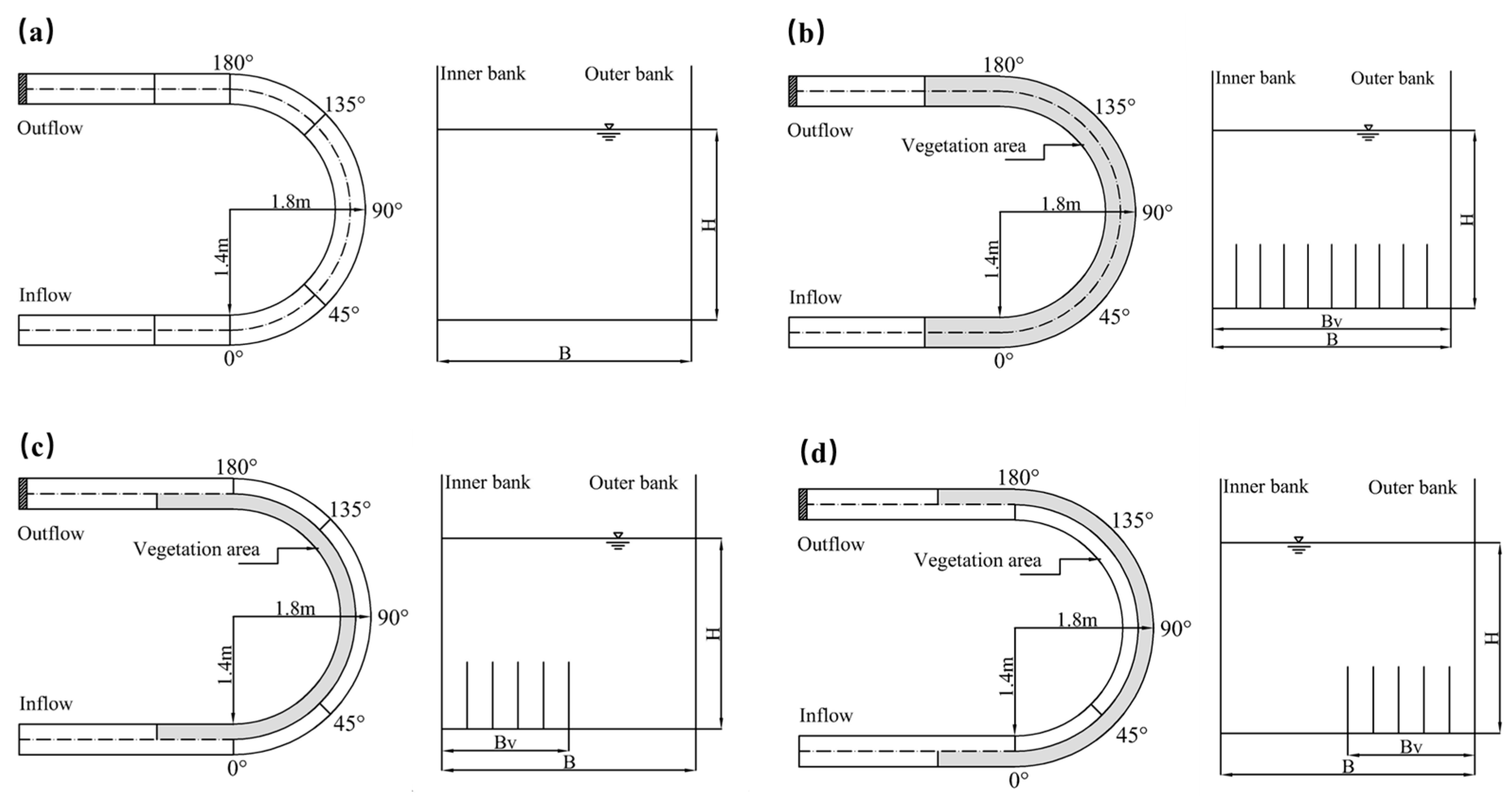
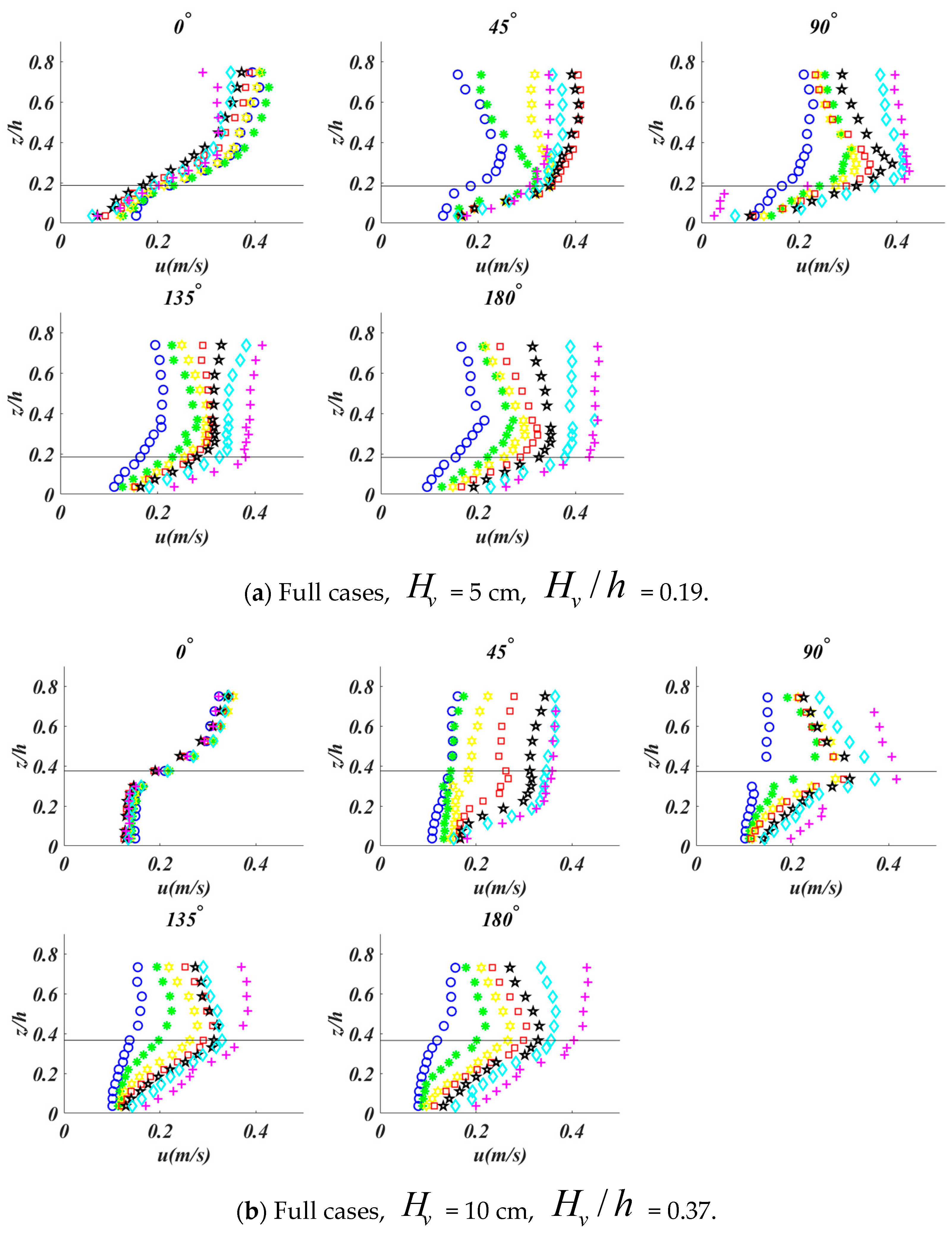
The longitudinal velocity distribution was fundamentally altered by the presence of submerged vegetation, with the specific pattern depending heavily on the vegetation configuration. Figure 4 shows the longitudinal velocities along the depth of each section in the full case, convex case, and concave case for Q = 0.030 m³/s when submerged vegetation height $H_v$ was 5 cm ($H_v/h$ = 0.19, Figure 3a) and 10 cm ($H_v/h$ = 0.37, Figure 3b), respectively. For the full case, at the 0° section (typically the straight section of the channel before the bend), the longitudinal velocity is lower in the vegetated area. In the non-vegetated area, the absence of additional resistance allows for higher longitudinal velocities. There is a velocity gradient and an obvious inflection point of velocity between the vegetation area and the non-vegetation area, which is basically located at the top of the vegetation area. For the case of taller vegetation ($H_v/h$ = 0.37), the vegetation drag leads to the constant longitudinal velocity profiles in the vegetated area at the 0° section. After entering the curved channel, longitudinal velocity profiles over the vegetation canopy are gradually affected by the centrifugal force along the channel bend, making the maximum velocity appear at the top of the vegetation area (black solid line), especially for the concave bank of the 90°, 135° and 180° sections for $H_v/h$ = 0.37. For both $H_v/h$ = 0.19 and $H_v/h$ = 0.37 cases, the vegetation canopy becomes the bottom boundary, and the curved channel effect mainly affects the flow field in the region above the vegetation areas. In addition, the bend channel effect appears at the 45° section for $H_v/h$ = 0.19, where the longitudinal velocities above the vegetation canopy become faster near the lower regions but slower near the water surface for y/B = 0.125 (○), a typical phenomenon for channel bend [20]. For $H_v/h$ = 0.37, the curved channel effect appears until the 90° section, indicating that the taller vegetation could delay the curved channel effect.

The longitudinal velocity distribution of submerged vegetation for $H_v/h$ = 0.37 at the 45° section has shown an obvious velocity gradient and maximum distribution. However, the longitudinal velocity distribution of submerged vegetation for $H_v/h$ = 0.19 does not change significantly, especially on the concave bank, which shows an obvious velocity gradient and maximum distribution at the 90° section. The results show that the height of submerged vegetation is reduced, and the longitudinal velocity is more affected by the curved channel than by the submerged vegetation.

Due to the centrifugal force along the channel bend, the longitudinal velocity is greater at the upper layer, and the velocity difference between the upper and lower vertical layers will be more significant when the lateral position is closer to the concave bank. For the full case with different heights (Figure 3a,b), at the 0° section, the characteristics of the longitudinal velocity distribution with $H_v/h$ = 0.19 are not as obvious as the case with $H_v/h$ = 0.37, especially in the concave bank, indicating that the vegetation height affects the longitudinal velocity distribution. Compared with the case where the vegetation height is 10 cm, it can be seen that the influence of the curved channel on the velocity of the vegetation height is a 5 cm delay. The longitudinal velocity distribution of submerged vegetation with a length of 10 cm at the 45° section has shown an obvious velocity gradient and maximum distribution. However, the longitudinal velocity distribution of submerged vegetation with a vegetation height of 5 cm does not change significantly, especially on the concave bank, which shows an obvious velocity gradient and maximum distribution at the 90° section. The results show that the height of submerged vegetation is reduced, and the longitudinal velocity is more affected by the curved channel than by the submerged vegetation.

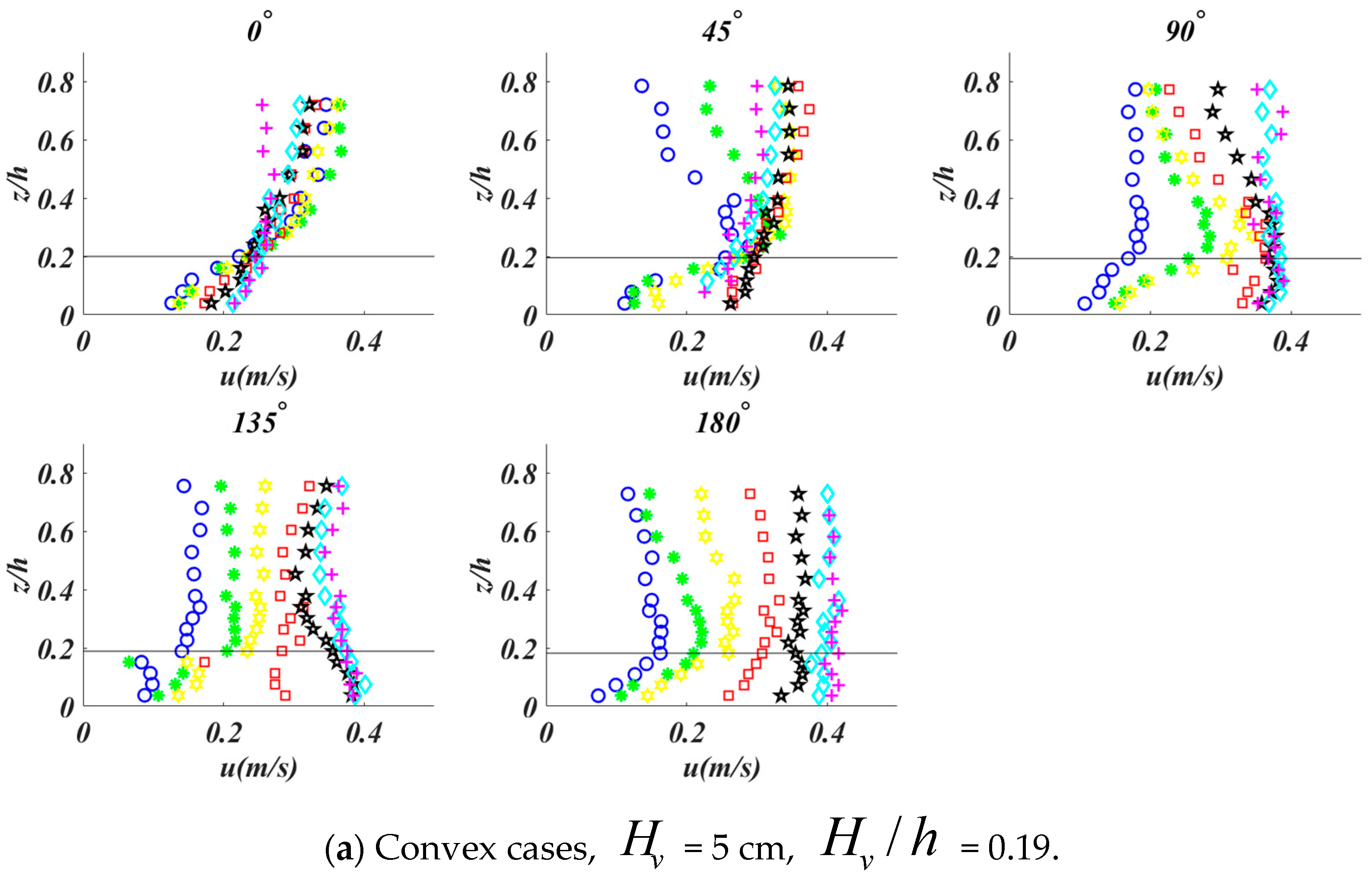
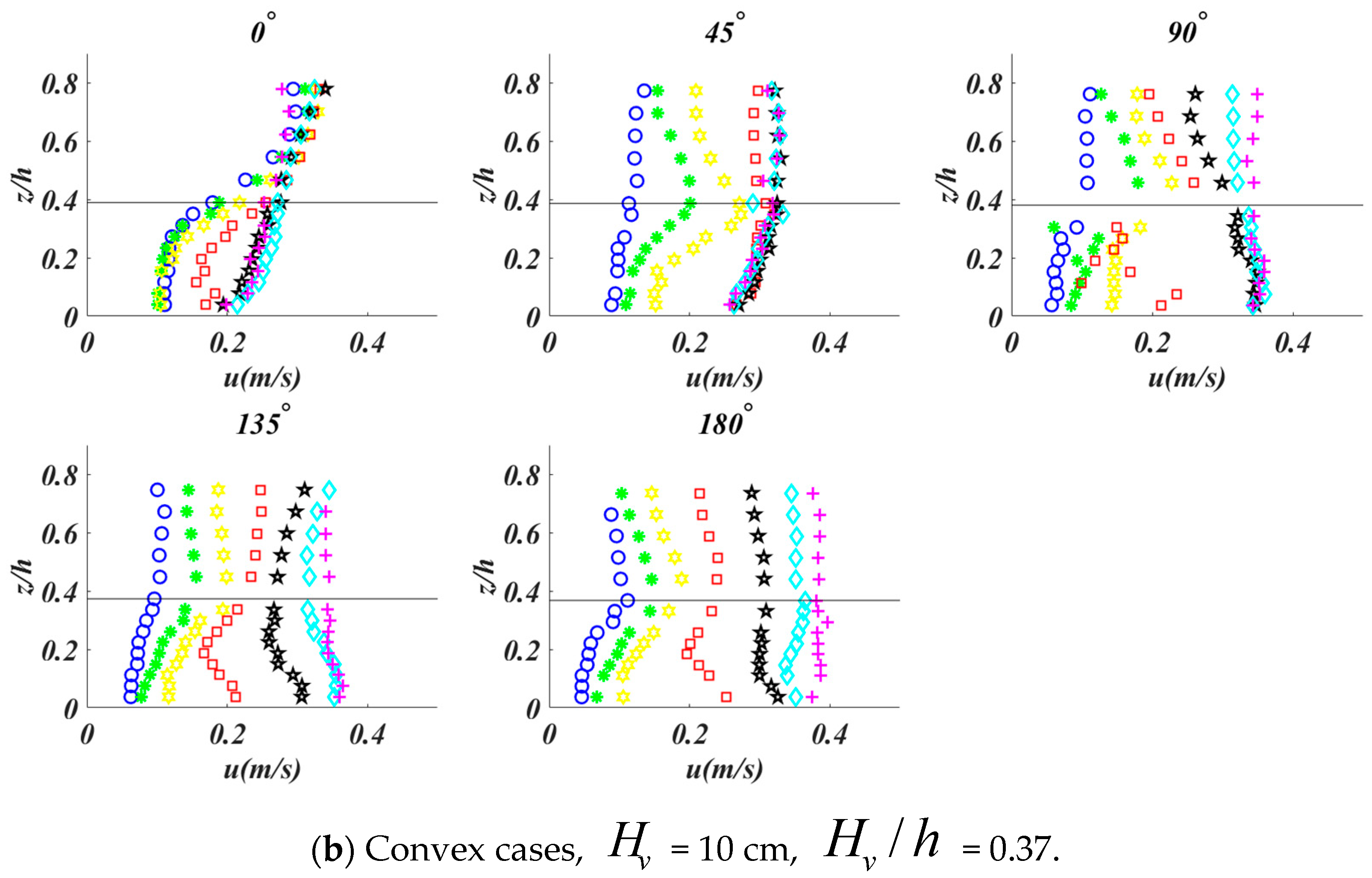
Figure 5 provides the longitudinal velocity profiles for the convex cases ($H_v/h$ = 0.19 and $H_v/h$ = 0.37). Similarly to the full cases, the curved channel effect appears above the vegetation canopy as the longitudinal velocity is faster near the vegetation canopy but slower near the water surface. For the shorter vegetation case ($H_v/h$ = 0.19), the curved channel effect appears from the innermost side to the outermost side. However, for the taller vegetation case ($H_v/h$ = 0.37), the curved channel effect mainly concentrates in the middle parts of the channel. After the channel bend, an obvious velocity gradient along the transverse direction will be formed for both cases. The transverse velocity gradient is greater for $H_v/h$ = 0.37 than for $H_v/h$ = 0.19. In addition, for $H_v/h$ = 0.19, the velocity at the top of the vegetation is greater than that for $H_v/h$ = 0.37 due to the decrease in vegetation height.

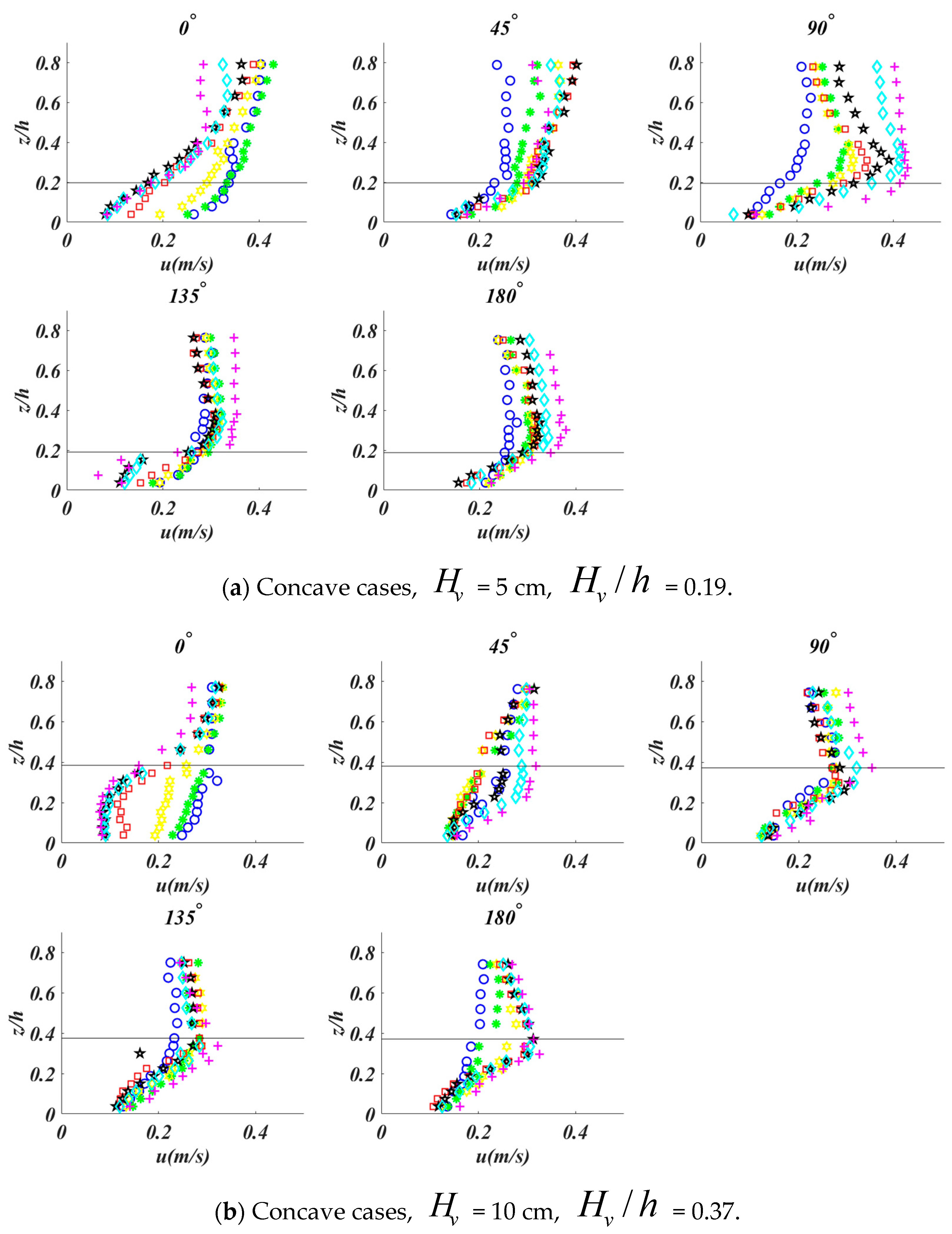
In the concave case (Figure 6), the longitudinal velocity distribution at the 0° section is similar to the convex case. After entering the curve, the velocity distribution is different from that of the convex case, which means there is no obvious transverse velocity gradient between the vegetated area and the non-vegetated area. This is because the curved channel without vegetation will increase the velocity on the concave bank and decrease the velocity on the convex bank, so the velocity on the convex bank decreases significantly and the velocity on the concave bank increases significantly in the convex case, which is prone to obvious transverse velocity gradient, while the velocity on the convex bank decreases slightly and that on the concave bank increases slightly in the concave case, resulting in no obvious transverse velocity gradient.

The main difference between the convex case and the full case is the difference in bottom velocity in the non-vegetation area; the velocities at $z/h$ = 0 of different transverse positions $y/B$ are different in the convex case, while they are almost the same in the full case. After entering the curved channel, the velocity in the upper part of the vegetation area gradually decreases, and the maximum value of the velocity appears at the top of the vegetation affected by the curved channel. In the non-vegetation area, the bottom velocity increases gradually, and the whole longitudinal velocity is in a linear distribution. The change in velocity in the transverse interface between vegetation and non-vegetation is more obvious. Affected by vegetation and bend circulation, it shows the characteristics of slower velocity in the lower part and faster velocity in the upper part. It is most obvious in the 90° section, 135° section, and 180° section, and an obvious velocity gradient along the transverse direction will be formed. The convex case of $H_v$ = 5 cm has the same trend as that of $H_v$ = 5 cm, while the velocity at the top of vegetation is greater due to the decrease in vegetation height.

3.2. Transverse Velocity Distribution

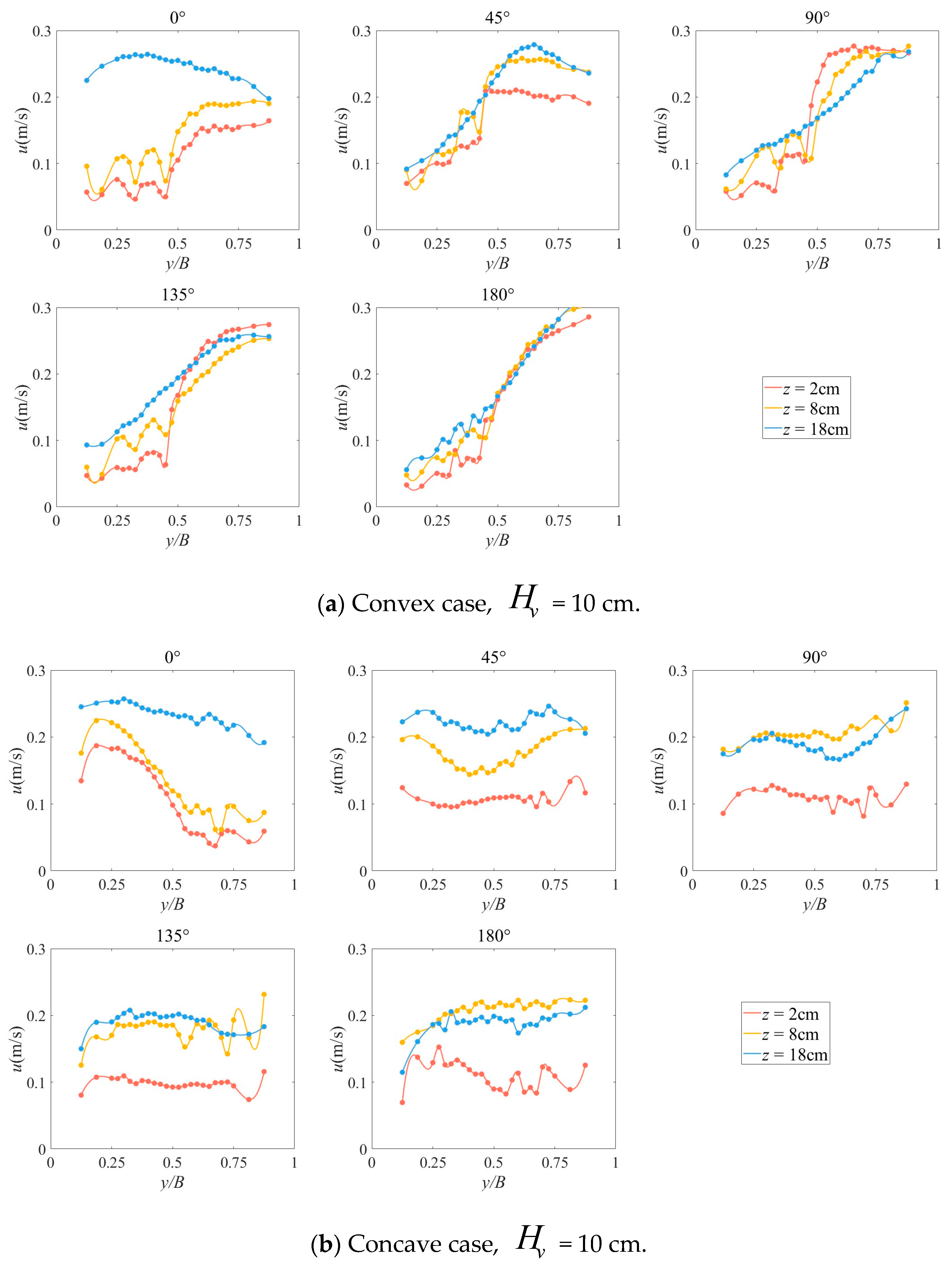
The variation in transverse velocity in the convex case with $H_v$ = 10 cm is shown in Figure 7. Three positions are taken for the measuring points, namely vegetation area ($z$ = 2 cm), vertical interface ($z$ = 8 cm), and non-vegetation area ($z$ = 18 cm). In the vegetation area at the 0° section, there is a velocity gradient in the transverse interface between vegetation and non-vegetation, and the velocity in the vegetation area decreases significantly due to the existence of vegetation on the convex bank. For the vertical interface, there is little difference in transverse velocity, and for the non-vegetation area, the velocity on the convex bank is slightly larger than that on the concave bank, which is consistent with the basic theory of curve hydraulics.

After entering the curve, the velocity on the convex bank decreases, and the velocity on the concave bank increases due to the influence of the centrifugal force of the curve. Therefore, in the non-vegetation area, the velocity on the convex bank decreases and the velocity on the concave bank increases, resulting in the trend of “low velocity on convex bank and high velocity on concave bank” in the transverse velocity distribution, and the trend will be more obvious when the time entering the curve is longer. The velocity in the vegetation area is affected by both the curved channel and vegetation, but the change in velocity is small. Therefore, the velocity difference in the vegetation area between the convex bank and concave bank gradually increases when entering the curve, indicating that the influence of submerged vegetation on the vegetation area is much greater than that of the curved channel.

3.3. Cross-Stream Circulation Distribution

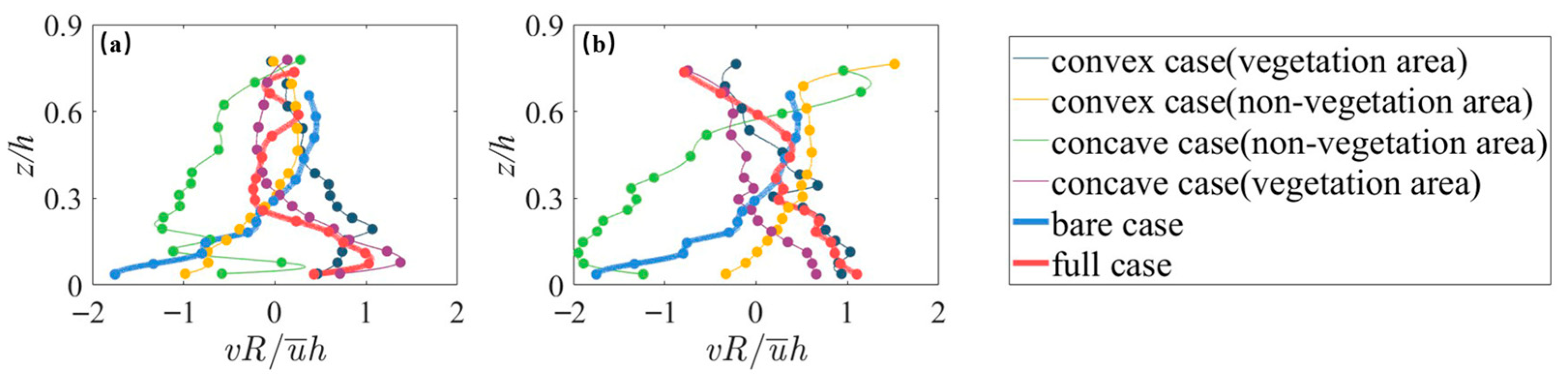
Secondary flow arising from centrifugal forces induced by streamline curvature is of considerable significance in meandering rivers [10]. Cross-stream circulation distributions serve as a reliable quantitative indicator for characterizing the magnitude of secondary flow. Figure 8 shows the cross-stream circulation distributions in the 90° section, where the X-axis is $vR/\left(\overline{u}h\right)$, the Y-axis is $z/h$, and $\overline{u}$ is the average longitudinal velocity. When the calculated $vR/\left(\overline{u}h\right)$ values distribute on the same side of $vR/\left(\overline{u}h\right)=0$, i.e., all $vR/\left(\overline{u}h\right)$ values are larger or smaller than zero, it means there is no secondary flow.

It can be seen from Figure 8 that no matter whether the vegetation height is 5 cm or 10 cm, there is obvious cross-stream circulation in the full case (red line) and the bare case (blue line) which is bold, but the direction of cross-stream circulation is reversed (the red line in Figure 7 is the cross-stream circulation under full case, and the blue line is the cross-stream circulation under the bare case, and the direction is reversed). Both the convex case and concave case exhibit a phenomenon in which the cross-stream circulation direction is the same as the bare case in the non-vegetation area, while the cross-stream circulation direction is the same as the full case in the vegetation area. Therefore, submerged vegetation will change the direction of the bend circulation. This may be due to the presence of submerged vegetation that causes changes in the distribution of lateral velocity, which is not related to the location of vegetation. The slope of cross-stream circulation is used to compare the secondary flow intensity. The slope with $H_v$ = 10 cm is greater than that with $H_v$ = 5 cm; it is indicated that the circulation intensity will be stronger with the increase in vegetation height under the presence of submerged vegetation, which is only related to vegetation height and has nothing to do with vegetation distribution.

3.4. Turbulent Kinetic Energy

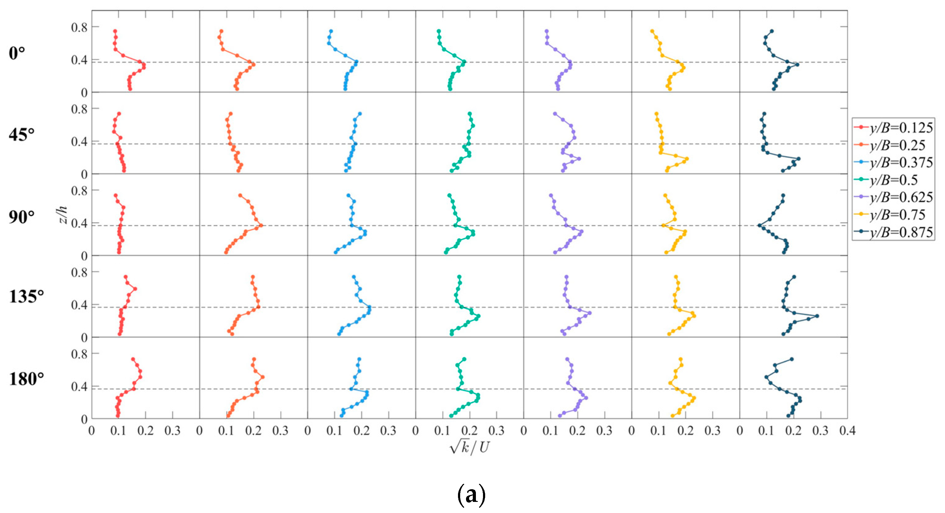
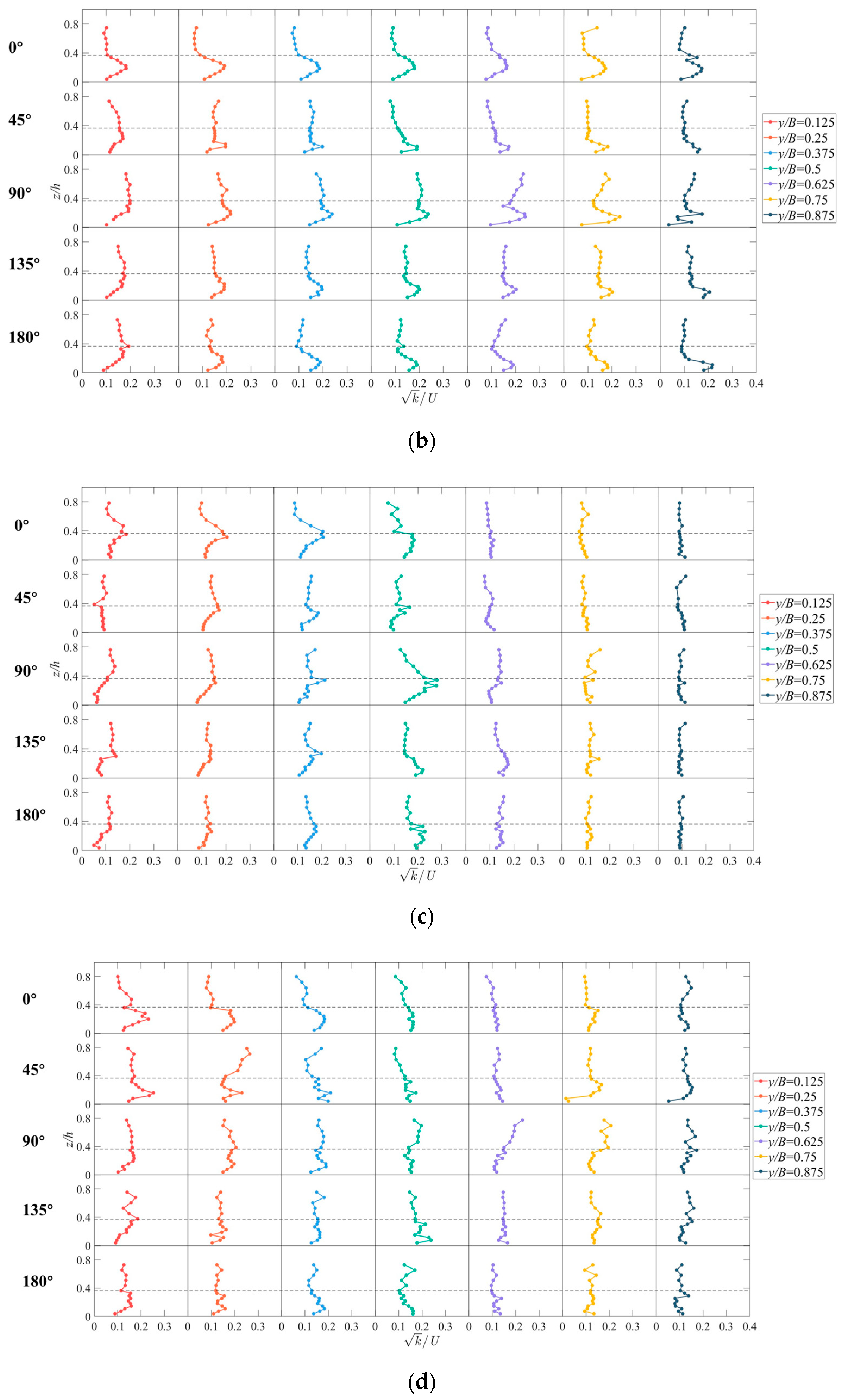
In this section, the turbulent kinetic energy is analyzed. The full case with different vegetation is shown in Figure 9a,b, and the turbulent kinetic energy is nondimensionalized by the section’s average velocity. At the 0° section, the turbulent kinetic energy has a maximum value along the water depth direction when the vegetation height is 10 cm. The wake caused by the flow passing through the vegetation strengthens the turbulence of the water body, strengthening the turbulent effect and turbulent kinetic energy. Because the attenuation of turbulent kinetic energy at the top of vegetation is faster than the vertical attenuation of longitudinal velocity, and the inflection point of longitudinal velocity appears at the top of vegetation, the maximum value of turbulent kinetic energy appears in the area slightly below the top of vegetation, where the turbulent effect is the strongest; the same findings were reported in the experimental results for the straight-channel flume. In addition, under the joint influence of the channel bend and the submerged vegetation, the attenuation of the turbulent kinetic energy at the top of the vegetation after entering the curve is faster than that at the 0° section and the maximum value of the turbulent kinetic energy moves down to nearly 1/3 of the vegetation height. The phenomenon of the maximum value of the turbulent kinetic energy in the middle line of the channel moving down is more obvious than that on the convex bank and concave bank. The distribution of the turbulent kinetic energy in the whole-channel bend is basically the same. When the vegetation height is 5 cm, the maximum value of turbulent kinetic energy appears in the top area of the vegetation, and the turbulence effect is the strongest in this area. The decrease in vegetation length makes the attenuation of turbulent kinetic energy at the top of the vegetation faster than that of longitudinal velocity, and the vertical attenuation effect is weakened.

In the convex case (Figure 9c,d), the turbulent kinetic energy reaches the maximum in the transverse interface at all sections. At the 0° section, the turbulent kinetic energy distribution in the vegetation area is the same as that in the full case, and the turbulence in the non-vegetation area is close to zero and has a linear distribution. The maximum TKE will appear in the transverse interface, which is affected by the turbulence in the vegetation area and the non-vegetation area, and the turbulence above and below the top of the vegetation. After entering the curve, the maximum value of turbulent kinetic energy decreases with the combined action of the curve and submerged vegetation, and falls from the top area of vegetation to the area with 1/2 of the vegetation height. 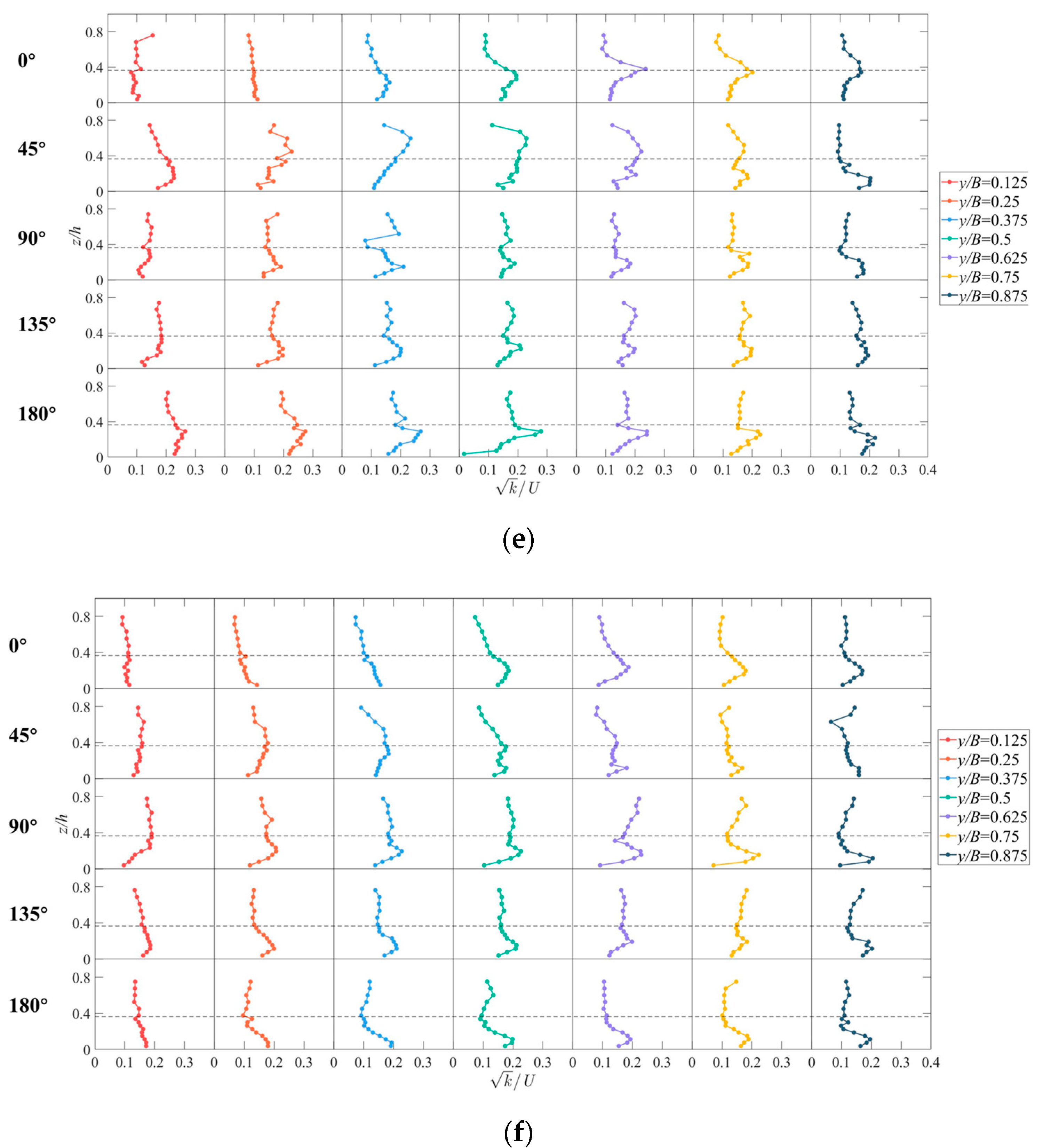In the concave case (Figure 9e,f), the same conclusion as that established for the convex case can be obtained at the 0° section. After entering the curve, the distribution of turbulent kinetic energy on the convex bank and concave bank is almost the same, and the maximum value of turbulence intensity moves slightly down from the top of the vegetation to the area with 2/3 of the vegetation height. Vegetation height has no obvious effect on the turbulent kinetic energy of the convex case and concave case.

In addition, compared with the full case, the turbulent kinetic energy in the non-vegetation area of the concave bank will be reduced in the convex case due to the influence of centrifugation, while the turbulent kinetic energy in the non-vegetation area of the convex bank will increase in the concave case. The different height of vegetation only affects the turbulent kinetic energy distribution for the 0° section, and the turbulent kinetic energy distribution in the curved channel is almost the same. In the case of submerged vegetation, the influence of the curved channel is stronger than that of vegetation. That means that the distribution of different vegetation groups has an effect on the turbulent kinetic energy of the section.

3.5. Spectrum Turbulent Spectral

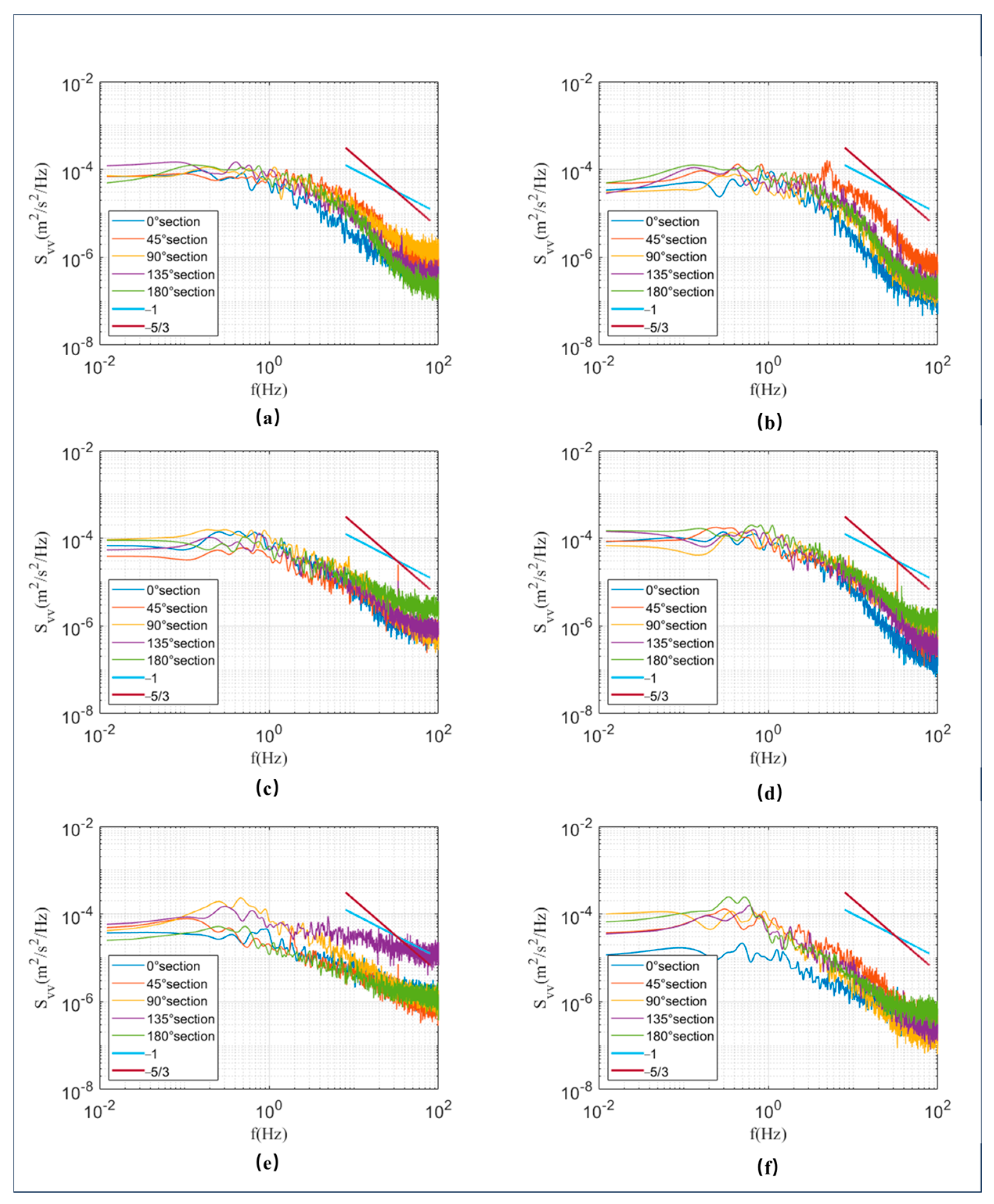
Spectral analysis of the transverse velocity fluctuations provided deeper insights into the turbulence structure [12]. Figure 10 presents the variation in the power spectral density (PSD) of instantaneous transverse velocity fluctuation against the frequency of five characteristic sections with submerged vegetation heights of 5 cm and 10 cm measured by ADVP with the sampling frequency of 100 Hz, where f represents the frequency, S_vv represents the turbulence spectrum distribution of transverse fluctuating velocity, and the moving average method is used to remove noise. The spectral analysis used here is based on the Welch method [34] with Hamming-type windowing [35]. 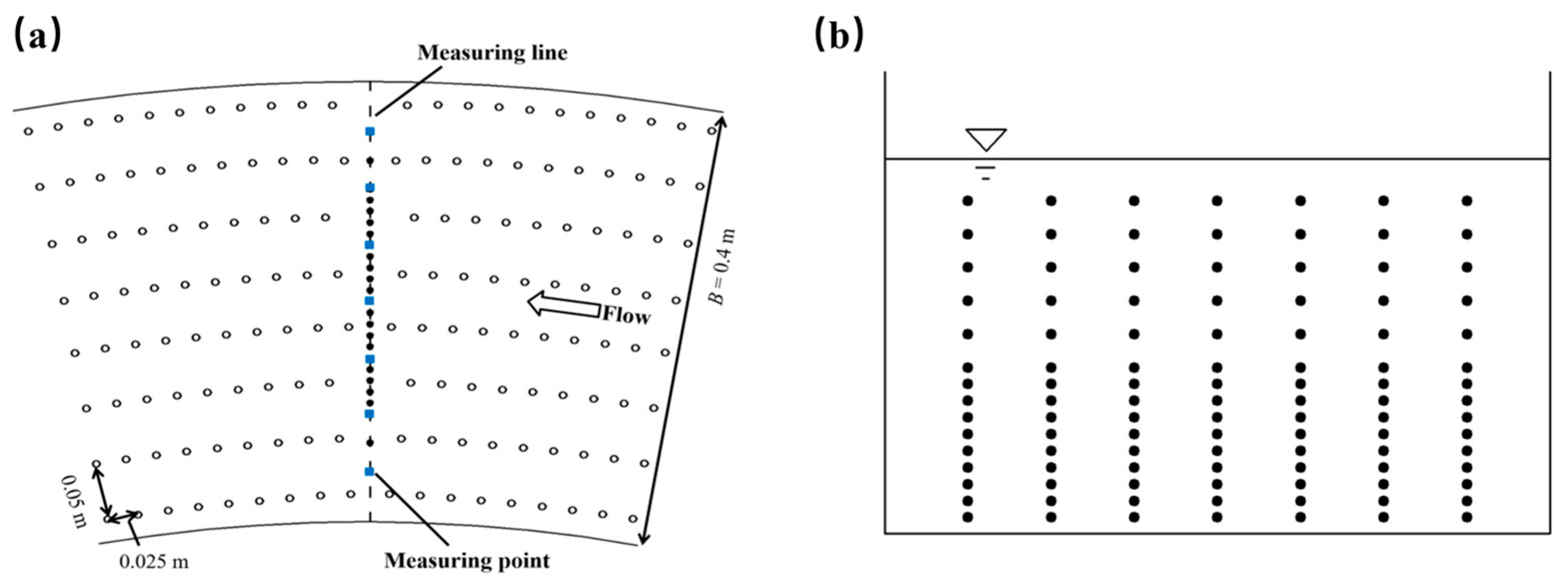In Figure 10, the feature points were measured at the mid-width (20 cm from the convex bank) of the flume of each characteristic section.

The full case can be vertically divided into three areas, namely the vegetation area, the vertical interface (vertical junction area between the vegetation and the non-vegetation), and the non-vegetation area. It can be seen from Figure 10 that in the vegetation area, the turbulence spectrum distribution of each section in the energetic area and the inertial subrange is relatively similar, indicating that vegetation is the dominant factor in the vegetation area, and the vortex structure of each section in the vegetation area is roughly the same. In the fully developed turbulence, the attenuation rate of the power density decays at a rate as Kolmogorov scaling (=−5/3); however, the attenuation rate of the power density at the curved section in Figure 10a is approximately −1 over a limited range due to the small turbulent vortices increase affected by the submerged vegetation. Huai and others have also obtained similar attenuation rate results for the inertial subrange. In the full case, the peaking frequency of the inertial sub area is not obvious, with a distribution of 0.4–0.8 Hz. In the dissipation area (f > 10¹ Hz), the turbulence spectrum is more vulnerable to the influence of the curve. As can be seen from Figure 9a, the slope of the dissipation zone of the 45–90° section is significantly greater than that of the 0° and 180° sections, indicating that the action of the curved channel will increase the dissipation of the turbulence spectrum in the vegetation area. At the same time, the difference in vegetation height also affects the dissipation rate of the dissipation zone which can be extrapolated from Figure 10b; this is because the higher the submerged vegetation height, the more transmission of water kinetic energy will be affected. The collision between water molecules and vegetation will be increased, the transmission efficiency of kinetic energy will be reduced, and the attenuation and dissipation of turbulent kinetic energy will be faster. And the dissipation of TKE will be promoted when the vegetation height increases.

In the vertical interface, it can be seen that the value of turbulence spectrum increases for the same vegetation height compared to the vegetation area, indicating that the turbulence kinetic energy is the strongest in the interface; this was also reported in the previous analysis results of turbulence kinetic energy. The attenuation rate of the inertial subrange of the 0° section is −5/3, while the attenuation rate of the inertial subrange of the curved section (45–180°) is approximately −1 over a limited range, indicating that there are more turbulent vortices in the vertical interface area of the curve, which has the greatest impact on the attenuation rate. Meanwhile, the peaking frequency of its habitual subrange is about 0.2 Hz, which is smaller than that of the vegetation area, indicating that the frequency of the dominant vortex structure decreases and the large turbulent vortex increases in the vertical interface. The dissipation of turbulent kinetic energy will be promoted by the increase in vegetation height, like the vegetation area.

In the non-vegetation area, the power spectral density value is the smallest of the three areas, indicating that the mixing is the weakest and the turbulence intensity is the lowest in the non-vegetation area. The attenuation rate of the inertial subrange is basically between Kolmogorov’s law (=−5/3) and −1, and the peak frequency of the inertial sub-region is about 0.2–0.3 Hz, which is between the peak frequency of the vegetation area and the vertical interface. Therefore, the frequency of the dominant vortex structure in the vertical direction is as follows: f (vegetation area) > f (vertical interface) > f (non-vegetation area). There are more large turbulent vortices in non-vegetation areas and more small turbulent vortices in vegetation areas. The smaller the peak frequency on the spectrum, the larger the size of the vortex.

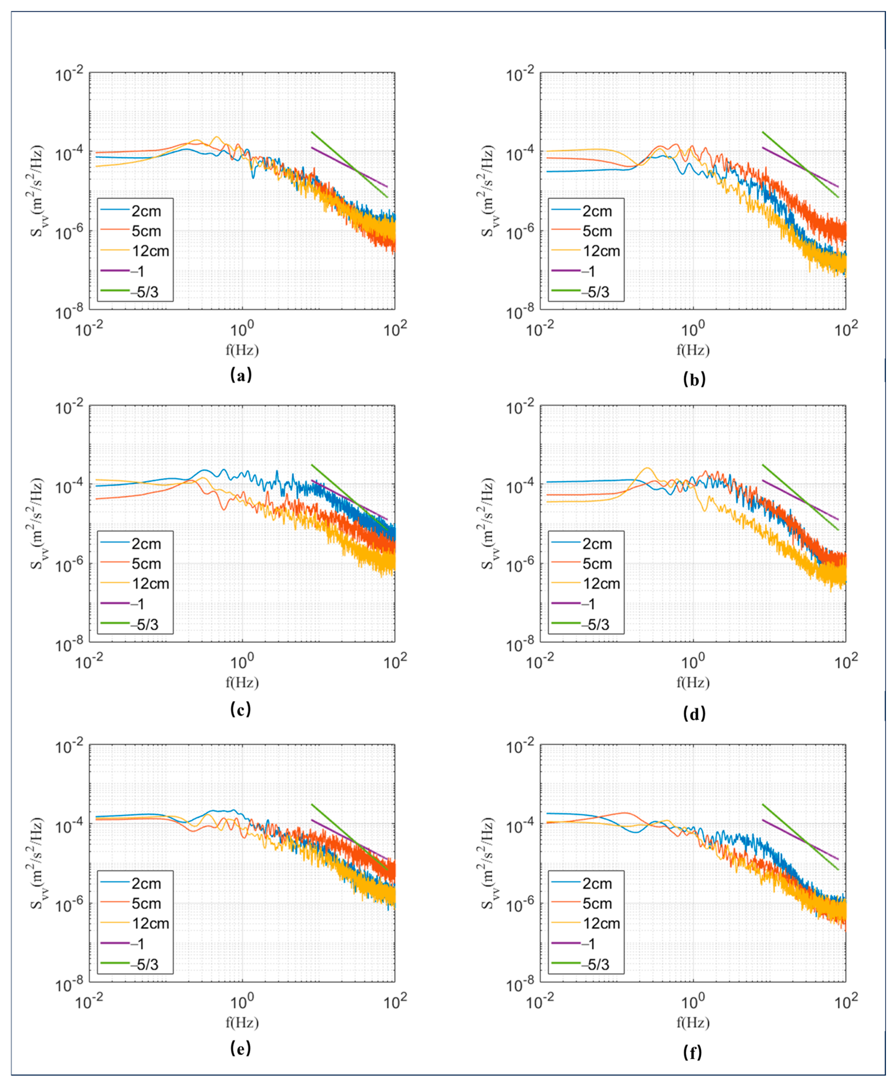
In order to study the influence of vertical position on turbulent flow spectrum in more depth, the vertical PSD distribution at different vegetation heights of the full case, convex case, and concave case is shown in Figure 11. All measuring points are at the transverse center line of the 90° section (20 cm from the convex bank). For the full case, the value of power spectral density S_vv in the vertical interface (red line) > S_vv in the vegetation area (blue line) > S_vv in the non-vegetation area (yellow line), and the peak frequency of turbulence spectrum is basically the same for the same vegetation height. As shown in Figure 11a, the peak frequency is about 0.4 Hz, indicating that the turbulence structure is basically the same, and the vertical position basically does not affect the distribution of the turbulence structure. For the convex case, the value of power spectral density S_vv in the vegetation area (blue line) > S_vv in the vertical interface (red line) > S_vv in the non-vegetation area (yellow line) when the vegetation height is 5 cm, while S_vv in the vertical interface (red line) is basically the same as that in the vegetation area (blue line) when the vegetation height is 10 cm. This is because there is not only a vertical interface but also a transverse interface between vegetation and non-vegetation, with vegetation on the convex bank. The impact of the transverse interface on the power spectral density is greater than that of the vertical interface when the vegetation length is low. Compared with the concave case, the velocity gradient of the convex case is larger due to the influence of the side vegetation and curve, and the mixing in the vertical interface is more intense. The power spectral density distribution of the convex case is higher than that of the concave case; however, the distribution positions of power spectral density spikes are the same, indicating that their turbulence structure is roughly the same. The different vegetation distribution only affects the turbulence intensity and has little effect on the turbulence structure.

In conclusion, vegetation and curve will enhance turbulence intensity and increase small turbulent vortices. The mixing will be increased in the transverse and vertical interface, making the turbulence stronger in the interface, and the phenomenon in the vertical interface will become more obvious. The difference in vegetation height mainly affects the dissipation rate of turbulence kinetic energy. The higher the height of vegetation, and the greater the number of collisions between water and vegetation, the lower the transfer efficiency of kinetic energy, and the faster the attenuation and dissipation of turbulence kinetic energy.

3.6. Turbulent Bursting

Turbulence bursting constitutes one of the key approaches for investigating near-bed coherent structures and sediment resuspension in open-channel flows [15]. Quadrant analysis is widely employed to quantify instantaneous Reynolds stress, thereby enabling the characterization of turbulent structures, and this method stands as the predominant technique for studying turbulence bursting. In quadrant analysis, the instantaneous fluctuations $u’\left(t\right)$ and $w’\left(t\right)$ can be divided into four quadrants (i = I, II, III, IV) according to the signs of the instantaneous velocity fluctuations, so the i-th quadrant can represent a turbulence event. i = I, u’ > 0, w’ > 0, outward interaction; i = II, u’ < 0, w’ > 0, ejection; i = III, u’ < 0, w’ < 0, inward interaction; i = IV, u’ > 0, w’ < 0, sweep.

In order to describe turbulent events accurately, a hole (instead of zero) is used to separate the Reynolds stress contributions. The hole is formed by four hyperbolas. $\left|u^{\prime }\left(t\right)w^{\prime }\left(t\right)\right|=G_0\left|u^{\prime }{w}^{\prime }\right|$, where G₀ is a threshold value. The contribution rate of each quadrant can be expressed as S_k (k = I, II, III, IV represent four quadrants):

$$S_k=\left\{\begin{array}{c}1,\left|u^{\prime }\left(t\right)w^{\prime }\left(t\right)\right|>G_0\left|u^{\prime }{w}^{\prime }\right|,\left[u^{\prime }\left(t\right){,w}^{\prime }\left(t\right)\right]inthesamequadrant\\ 0,otherwise\end{array}\right.$$

(4)

This paper sets the threshold to G₀ = 1.0. Therefore, the frequency f_k of each turbulence, once event-corrected, can be expressed as follows:

$$f_k={\displaystyle \frac{{\sum }_{t=0}^T{S}_k}{{\sum }_{t=0}^T{S}_I+{\sum }_{t=0}^T{S}_{II}+{\sum }_{t=0}^T{S}_{III}+{\sum }_{t=0}^T{S}_{IV}}}$$

(5)

where T is the length of measurement time.

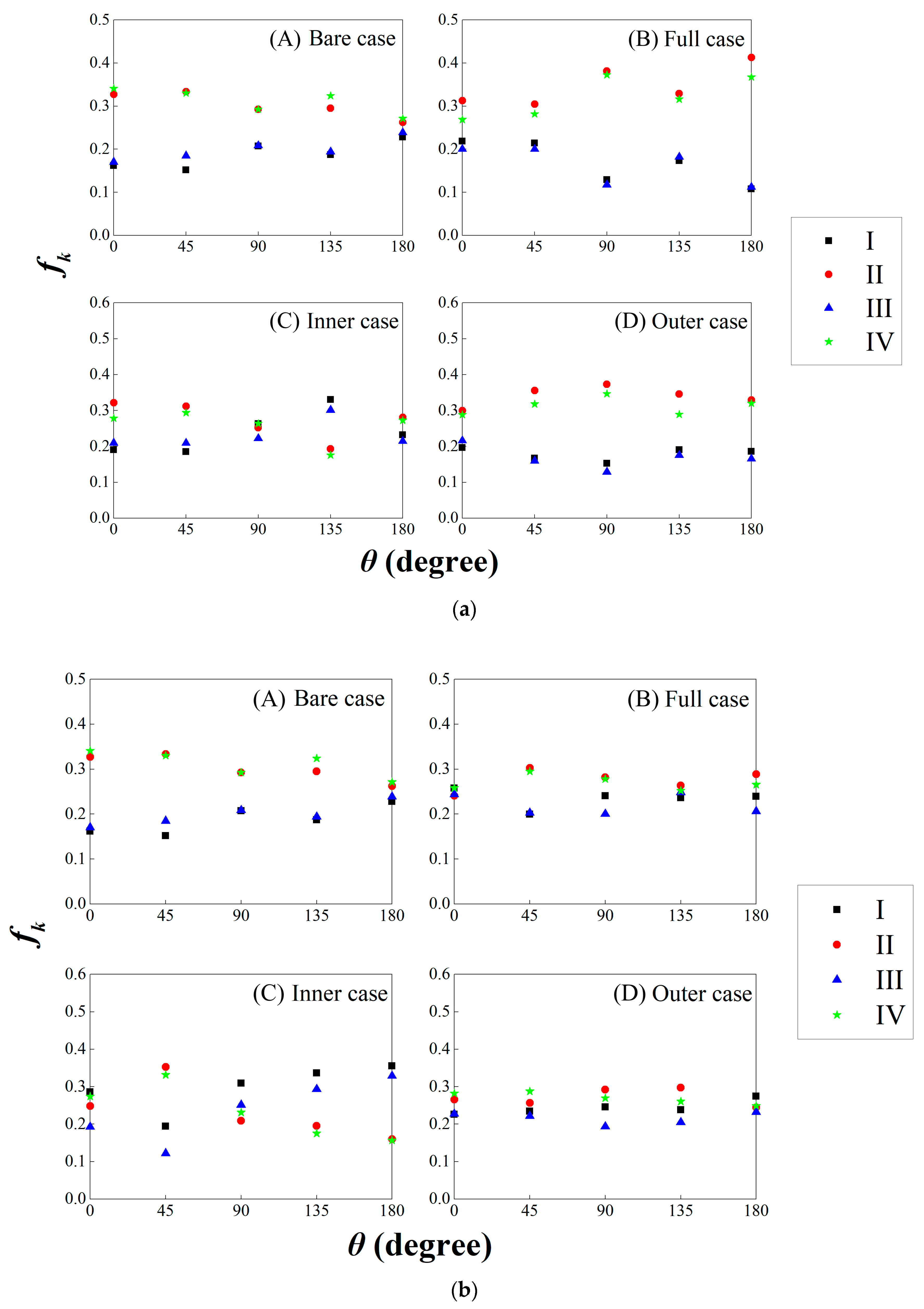
Figure 12 presents the distribution of the occurrence frequency f_k of four turbulence events across different vegetation heights and experimental cases. In the bare channel scenario, the occurrence frequencies of ejection and sweep events (events II and IV) at the 0° cross-section are higher than those of outward and inward interaction events (events I and III). This indicates that the upward migration of low-velocity fluid and downward movement of high-velocity fluid constitute the dominant flow processes, which aligns with the findings of Afzalimehr et al. [36] and Yager & Schmeekle [37] in straight open channels. Beyond the 45° cross-section, the intensities of outward and inward interaction events (events I and III) gradually intensify, persisting until the 180° cross-section, where the occurrence frequencies of the four turbulence events become roughly equivalent. This observation confirms that channel curvature enhances the magnitude of outward and inward interaction events, likely attributed to the strengthened wall rebound of high-velocity fluid and reverse thrust of low-velocity fluid—factors that amplify turbulent interactions within the main flow.

For the full case, the occurrence frequency of ejection and sweep at the 0° section is still higher than the outward interaction and inward interaction when the vegetation height is 5 cm (H_v/h = 0.19), while the difference between the occurrence frequency becomes smaller when compared with the bare case, indicating that the existence of submerged vegetation will increase the frequency of the outward interaction and inward interaction. For the case with a vegetation height of 10 cm (H_v/h = 0.37), the occurrence frequencies of the four turbulence events are basically the same, indicating that the wall rebound of high-speed fluid and the reverse thrust of low-speed fluid will be increased, and the existence of vegetation will enhance the interaction of turbulence when the vegetation is taller. After entering the curve, the occurrence frequency of ejection and sweep will continue to increase in the case with vegetation height of 5 cm, while the occurrence frequencies of the four turbulence activities are constant in the case with a vegetation height of 5 cm, indicating that the contribution of the four turbulence events is basically the same when the vegetation height is relatively high.

For the convex case, the frequency of ejection and sweep gradually decreases in the process of the curve when the vegetation height is 5 cm (H_v/h = 0.19), and the frequency of outward interaction and inward interaction gradually increases in the process of the curve, and the trend is more obvious when the vegetation height is 10 cm (H_v/h = 0.37). For the concave case, the frequency distribution of the four turbulence events in the curved channel is consistent with that in the full case, which shows that the convex bank is more vulnerable to the influence of curve action, while the concave bank is more vulnerable to the influence of submerged vegetation.

3.7. Reynolds Stress

Reynolds stress is the shear stress generated between the flow layers due to the exchange of turbulent water masses [16]. The physical significance is the energy transfer caused by the uneven distribution of velocity in the flow field due to the occurrence of turbulence. The Reynolds stress distribution is mainly used to evaluate the shear velocity; that is, the resistance of the bottom bed to the fluid. In the case of half-side vegetation, the distribution of Reynolds stress will become more complex.

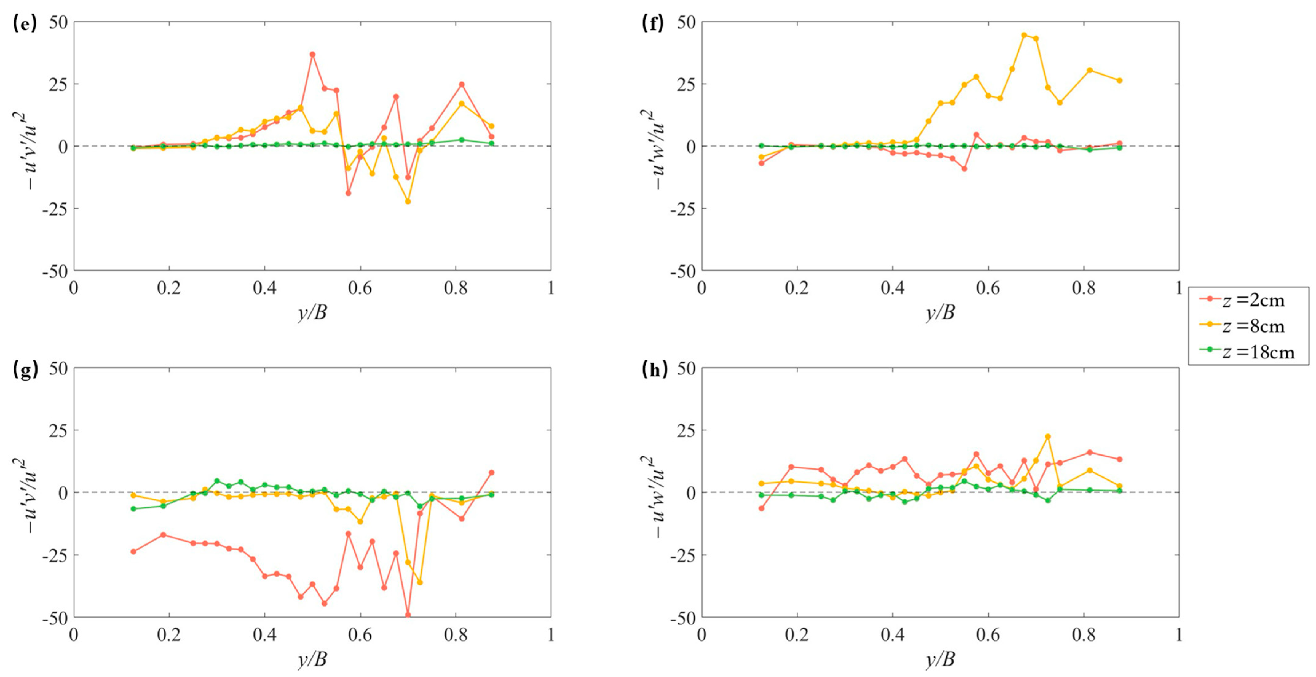
The transverse transmission ($-\overline{u\prime v\prime }$) and vertical transmission ($-\overline{u^{\prime }{w}^{\prime }})$ of straight section (0°) and the curve section (90°) are analyzed, respectively. To enhance the clarity of the trend, the transverse transmission ($-\overline{u\prime v\prime }$) and vertical transmission ($-\overline{u^{\prime }{w}^{\prime }})$ were normalized by ${u^{\prime }}^2$. 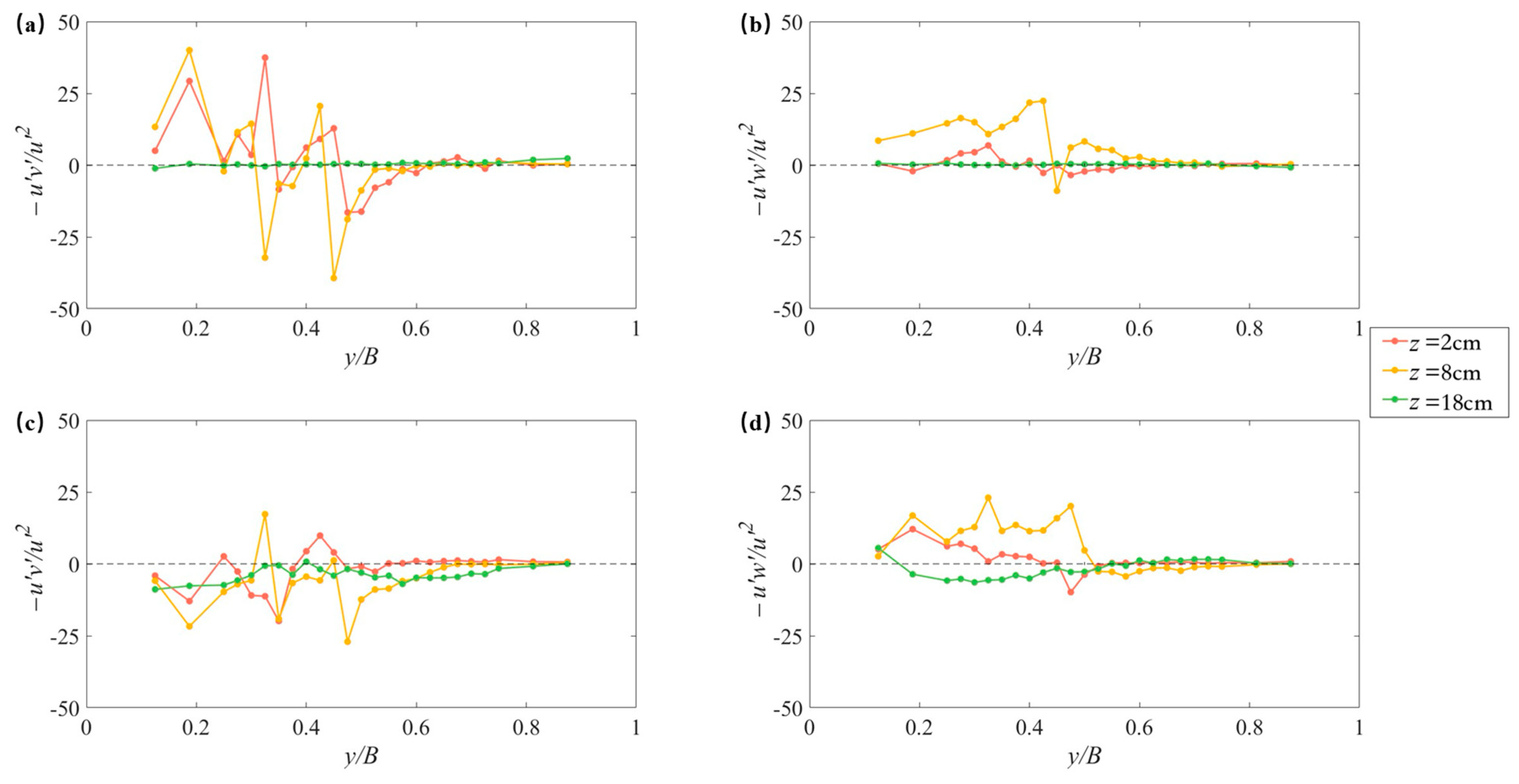The case with vegetation height of 10 cm is taken as an example, as the influence of vegetation height on Reynolds stress distribution is not significant. The transverse distribution of vertical transmission and the transverse transmission convex case and concave case is shown in Figure 13, in which the dotted line represents the transverse interface between the vegetation and non-vegetation area.

It can be seen from Figure 13a,b that in the 0° section of the convex case, the turbulent transport of momentum $-\overline{u\prime v\prime }$ and $-\overline{u^{\prime }{w}^{\prime }}$ in the non-vegetation area is approximately near zero, indicating that the main areas of turbulent momentum transport are concentrated in the vegetation area and the interface, and there is little transport in the non-vegetation area. For the interface, the vertical transport of momentum $-\overline{u^{\prime }{w}^{\prime }}$ in the convex bank is intense, but the maximum value of transverse transport of momentum $-\overline{u\prime v\prime }$ occurs at the transverse interface, indicating that the transverse momentum transport is most intense at the transverse interface. For the vegetation area, the vertical transport of momentum is basically near zero, but the transverse transport of momentum increases first and then decreases, reaching a maximum at the transverse interface. At the 90° section, as shown in Figure 13c,d, the trend of Reynolds stress in the vegetation area is similar to that of the 0° section. The vertical transport of momentum is the main change in the interface. The vertical momentum transport is greater than 0 in the convex bank with vegetation and less than 0 in the concave bank without vegetation. The vertical transport momentum direction of the convex bank and concave bank is reversed, while the transverse transport momentum is always the largest at the transverse interface because the function of the curved channel increases the maximum value of the transverse transport of momentum. The non-vegetation area is greatly affected by the curved channel and has obvious transverse and vertical transport of momentum, but its Reynolds stress value is still less than that in the interface and vegetation area. Therefore, the influence of the curved channel in the non-vegetation area is much greater than that in the vegetation area.

For the concave case (Figure 13c,d), the transverse transport of momentum and vertical transport in the non-vegetation area are close to zero at the 0 section, which is similar to the convex case. For the interface, the maximum value of $-\overline{u\prime v\prime }$ occurs at the interface, which is the same as the convex case, while the direction of transverse momentum transport is opposite to that in the convex case due to the different vegetation positions. For the vegetation area, the vertical and transverse distributions of turbulent momentum transport are the same as the convex case, but the transport direction is reversed, just like the interface. At the 90° section, the transverse transport of momentum in the vegetation area first increases and then decreases, and the maximum value is obtained at the transverse interface. However, compared with the 0° section and convex case, the maximum value is greater, indicating that the transverse transport of momentum is more intense when the vegetation is arranged on the concave bank, and the value of $-\overline{u^{\prime }{w}^{\prime }}$ is greater than zero. The vertical transport in the interface is positive, while the transverse transport is always the largest at the transverse interface, and the maximum value of transverse transport increases due to the action of the curved channel.

4. Conclusions

This experimental study systematically elucidates the profound effects of rigid submerged vegetation on the hydrodynamic characteristics of flow in a strongly curved 180° channel. The key findings are summarized as follows:

The presence of submerged vegetation significantly dampens the flow velocity within the vegetated zone, creating a distinct velocity shear layer at the vegetation canopy. The centrifugal force induced by the channel bend redistributes the longitudinal velocity, pushing the maximum velocity to the top of the vegetation canopy in the downstream sections. The onset of this curvature effect was delayed with increasing vegetation height, indicating that taller vegetation has a greater influence on the flow field in the initial bend sections.

Vegetation configuration critically influences the transverse flow structure. In partially vegetated cases (convex/concave), a pronounced transverse velocity gradient developed between vegetated and non-vegetated areas. More importantly, submerged vegetation was found to alter the direction of secondary circulation. The cross-stream circulation within vegetated areas exhibited the opposite rotation to that in bare channels. The intensity of this circulation strengthened with increasing vegetation height, independent of its lateral distribution.

The TKE profiles were characterized by a maximum value located slightly below the vegetation canopy top, associated with strong shear generation. The interaction between the bend and the vegetation caused the vertical position of the maximum TKE to descend towards the mid-canopy level in the curved sections. The strongest turbulence was consistently observed at the vertical and transverse interfaces between vegetated and non-vegetated zones.

Spectral analysis of transverse velocity fluctuations indicated that vegetation and channel curvature enhance small-scale turbulence. The inertial subrange slope in vegetated regions and interfaces deviated from the typical −5/3 law, approaching −1 over a limited range, suggesting an increased population of small turbulent vortices. The dominant vortex frequency was highest in the vegetation area and lowest in the non-vegetation area. Higher vegetation density promoted a faster dissipation of turbulent kinetic energy.

Quadrant analysis revealed that submerged vegetation alters the coherent structure of turbulence. While ejection and sweep events dominated in the bare and sparsely vegetated cases at the inlet, the presence of taller vegetation led to a more balanced distribution of all four turbulent events (ejection, sweep, outward, and inward interactions), enhancing turbulent mixing. The convex bank configuration was more susceptible to curvature-induced changes in bursting events. However, the quadrant statistics may be sensitive to the threshold, particularly in a vegetated interface where events may be intermittent.

The transport of momentum, quantified by Reynolds stresses, was most intense at the vegetation–non-vegetation interfaces. The channel curvature amplified the transverse momentum transport, with the maximum values observed at the transverse interface. The direction and magnitude of momentum transport were highly dependent on the vegetation placement (convex vs. concave bank), with the concave bank vegetation configuration inducing the most intense transverse momentum exchange.

In conclusion, this research underscores the complex, multifaceted interactions between rigid submerged vegetation and the flow in a sharply curved channel. The vegetation height, density, and spatial distribution are pivotal factors that collectively govern the flow resistance, velocity redistribution, turbulence generation, and momentum transport. These insights are critical for advancing the predictive modeling of natural vegetated rivers and for informing effective and sustainable river restoration and management practices. However, more complex (flexible and foliated) vegetation exists in real aquatic environments and behaves differently from the rigid and submerged vegetation in flows. In future work, numerical simulation should be realized to compare with experimental data. Also, field measurements should be conducted to validate and extend the laboratory-scale findings reported in this study. For quadrant analysis, error bars or confidence intervals should be shown to indicate the sensitivity to the threshold.