Monthly Streamflow Forecasting for the Irtysh River Based on a Deep Learning Model Combined with Runoff Decomposition

Abstract

The mid- and long-term hydrological forecast is important for water resource management and disaster prevention. Moreover, mid- and long-term hydrological forecasts in the region with poorly observed field meteorological data are a great challenge for traditional hydrological models due to the complexity of hydrological processes. To address this challenge, a machine learning model, particularly the deep learning model (DL), provides a new tool for improving the accuracy of runoff prediction. In this study, we took the Irtysh River, one of the longest rivers in Central Asia and a well-known trans-boundary river basin with poor field meteorological observations, as an example to develop a deep learning model based on LSTM and combined with runoff decomposition by Maximal Overlap Discrete Wavelet Transform (MODWT) to process target variables for predicting monthly streamflow. We also proposed an XGBoost-SHAP (Extreme Gradient Boost-SHapley Additive Explanations) method for the identification of predictors from large-scale indices for the streamflow forecast. The results suggest that MODWT shows the robustness of runoff decomposition between the training and test period. The deep learning model combined with MODWT shows better performance than the benchmark deep learning model without MODWT illustrated by an increased NSE. The XGBoost-SHAP method well identified the nonlinear relationship between the predictors and streamflow, and the predictors determined by XGBoost-SHAP can be physically explained. Compared with the traditional mutual information method, the XGBoost-SHAP method improves the accuracy of the deep learning model for streamflow forecast. The results of this study illustrate the ability of a deep learning model for mid- and long-term streamflow forecast, and the methods we developed in this study provide an effective approach to improve the streamflow prediction in the scarcely observed catchments.

1. Introduction

Floods and droughts can cause enormous economic and social losses, and they are becoming more frequent and severe in response to the global climate change. Accurate mid- and long-term runoff forecasts are of great utility as they benefit the planning of water resources, as well as the management of reservoirs and reductions in flood damage. Due to the complexity of watershed hydrological systems, there are knowledge gaps for understanding the hydrological processes in current hydrological sciences. Particularly, for the hydrological regime in the poorly field observed region, such as cold region catchments influenced by cryospheric components including permafrost, snow packs, and glaciers, there is a great challenge for hydrological predictions regarding the physically based model. Machine learning (ML), particularly deep learning (DL), enhances hydrological forecasting by leveraging data-driven approaches to model complex, nonlinear relationships in hydrological processes, improving prediction accuracy for streamflow and flood events. Methods that can improve the generalization ability and prediction accuracy of the ML model, such as combining the runoff decomposition method of ML and a reasonable selection of predictors, are also receiving an increase in investigations [1,2]. Therefore, it is important to study the methods that can enhance the performance of ML models for hydrological forecasts, particularly in the watershed with poor field meteorological observations [3,4].

The approaches of hydrological forecast can be classified into two categories including the data-driven model and process-driven model [5]. The conceptual hydrological models that lie between the two are ineffective when dealing with complex hydrological regimes in river basins. However, when increasing the complexity of the models, they encounter significant uncertainties [6,7]. The process-driven model is characterized by well-defined physical processes, and it can lead to reliable streamflow forecasts when combined with predicted meteorological variables [8,9,10,11,12]. However, it requires a substantial quantity of high-quality input data in order to achieve optimal results, such as land-use, soil, and meteorological data; therefore, it usually shows poor performance in scarcely observed regions. Compared with the process-driven model, the data-driven model can obtain acceptable results with low requirements of data, high computational efficiency, and a relatively simple model framework. The traditional data-driven model is usually based on the statistical relationship between predictors and the target variable, such as streamflow. For example, the commonly used autoregressive time series model, the autoregressive integral moving average model [13], requires only runoff data for prediction. Multiple linear regression and various models based on Bayesian methods are still widely used today [14,15]. Traditional statistical methods for hydrological forecasting often struggle with insufficient amounts of data and high-dimensional inputs, leading to limited accuracy in capturing complex hydrological processes [16]. To deal with these challenges, ML models have received more attention in recent decades. The ML model gives us a new perspective to solve these difficulties because it can better capture the potential relationship from limited data [17]. Although ML models provide a new perspective to capture complex relationships, their performance remains constrained by the non-stationarity and noise interference in raw streamflow data [18]. For instance, the direct application of ML to the original runoff series often results in overfitting to high-frequency fluctuations while missing long-term trends [19]. To address this, signal decomposition techniques have emerged as a critical preprocessing step. Among them, MODWT demonstrates unique advantages due to its multi-analysis resolution capability and ability to preserve information during decomposition. Zhang et al. [20] compared the performance of machine learning methods combined with EMD, VMD, and WT methods in predicting daily runoff at the Huanren Station, China. They indicated that the runoff decomposition methods can effectively enhance the performance of runoff prediction. Compared with EMD, VMD, and WT, MODWT has advantages in terms of stability, computational efficiency, and flexibility in signal decomposition, and it is particularly suitable for processing runoff data containing multi-scale signals. However, there are still some challenges for the decomposition method; for example, the problem of information leaking [21] causes the decomposition of data in the train and test period together, which means that the train of the model is not independent from the data in test period. Therefore, it is important to study the hybrid method combining the ML model with the decomposition approach, for example, to deal with the problem of information leaking.

On the other hand, the accuracy of medium- and long-term forecasts using data-driven models is highly dependent on the quality of predictors [22]. For a data-driven model, astronomical factors [23], the atmospheric circulation index [24], ocean thermal conditions, and watershed landscape, etc., are commonly used as predictors. Particularly, ENSO has significant influence on the global hydrological cycle [25,26], and it has been considered as a predictor of rainfall and streamflow in many regions [27,28,29]. However, for the large number of indices, they need to be further screened and selected to obtain reasonable input for models. Zhou et al. [30] compared three predictor selection methods in the western Tianshan Mountains and found that the best method for predictor selection was the mutual information method. Liao et al. [31] used the maximum information coefficient to select predictors. The precision and robustness of the forecast model is significantly influenced by the quality of the predictor recognition algorithm. Previous commonly used identification methods rely on linear correlation and fail to account for the nonlinear effects of predictors on streamflow, highlighting the requirement for more comprehensive approaches that address the nonlinear complexities.

In this study, we first propose a deep learning model combining the runoff decomposition method for monthly streamflow forecast. Then, we develop a method based on the predictors obtained by interpretable ML for hydrological forecast. Finally, the model was tested in a large transboundary river basin in the cold region, the Irtysh River Basin, where available field meteorological observation data are scarce. The results demonstrate that the proposed predictor selection method and the runoff prediction model can improve the mid–long-term runoff forecast.

2. Study Area and Data

2.1. Study Area

The Irtysh River is the largest tributary of the Ob River, which ultimately flows into the Arctic Ocean (Figure 1). Originating from the southern slopes of the Altai Mountains in Xinjiang province, China, the river flow northwestward, traversing the southern foothills of the Altai Mountains into Kazakhstan. It subsequently flows into Russia, where it converges with the Ob River at Khanty-Mansiysk. The river extends for a distance of 4248 km with a basin area of 1,643,000 km².

2.2. Data

Monthly observed runoff data at the Omsk and Tobolsk stations in Russia are obtained from the Global Runoff Data Centre (https://portal.grdc.bafg.de/applications/public.html?publicuser=PublicUser#dataDownload/Subregions (accessed on 1 September 2023)) [32]. These are target data and the output of models. Omsk is the midstream station, and Tobolsk is the station at the downstream of the river. The monthly runoff data are available from January 1951 to December 2012. In our study, the percentage of the data amount for the train and test dataset is 7:3. The runoff data were partitioned into a training set covering the year from 1951 to 1994 and a test set from 1995 to 2012.

Because the high quality of field observed in the Irtysh River was not available, large scale indices were used as predictors for the ML model. These are input data of the models. The distribution of the values of input data is shown in Figure 2. We obtained a dataset of the monthly climate index from the National Climate Centre of the China Meteorological Administration (http://cmdp.ncc-cma.net/Monitoring/cn_index_130.php (accessed on 10 September 2023)). This dataset includes 26 sea surface temperature indices (SST), 88 atmospheric circulation indices (AC), and 16 other indices. The raw data are in table form and stored in .csv format. These data are available from 1951 to 2012, which is the same period as the runoff data. We removed the indices with missing records greater than 30% of the total months and filled in the missing values in the remaining data using linear interpolation. The changes in these climate indices are gradual. Therefore, it is reasonable to use linear interpolation, and an example of the North African Subtropical High Ridge Position Index is shown in Figure S1 in the Supplemental Material.

3. Methodology

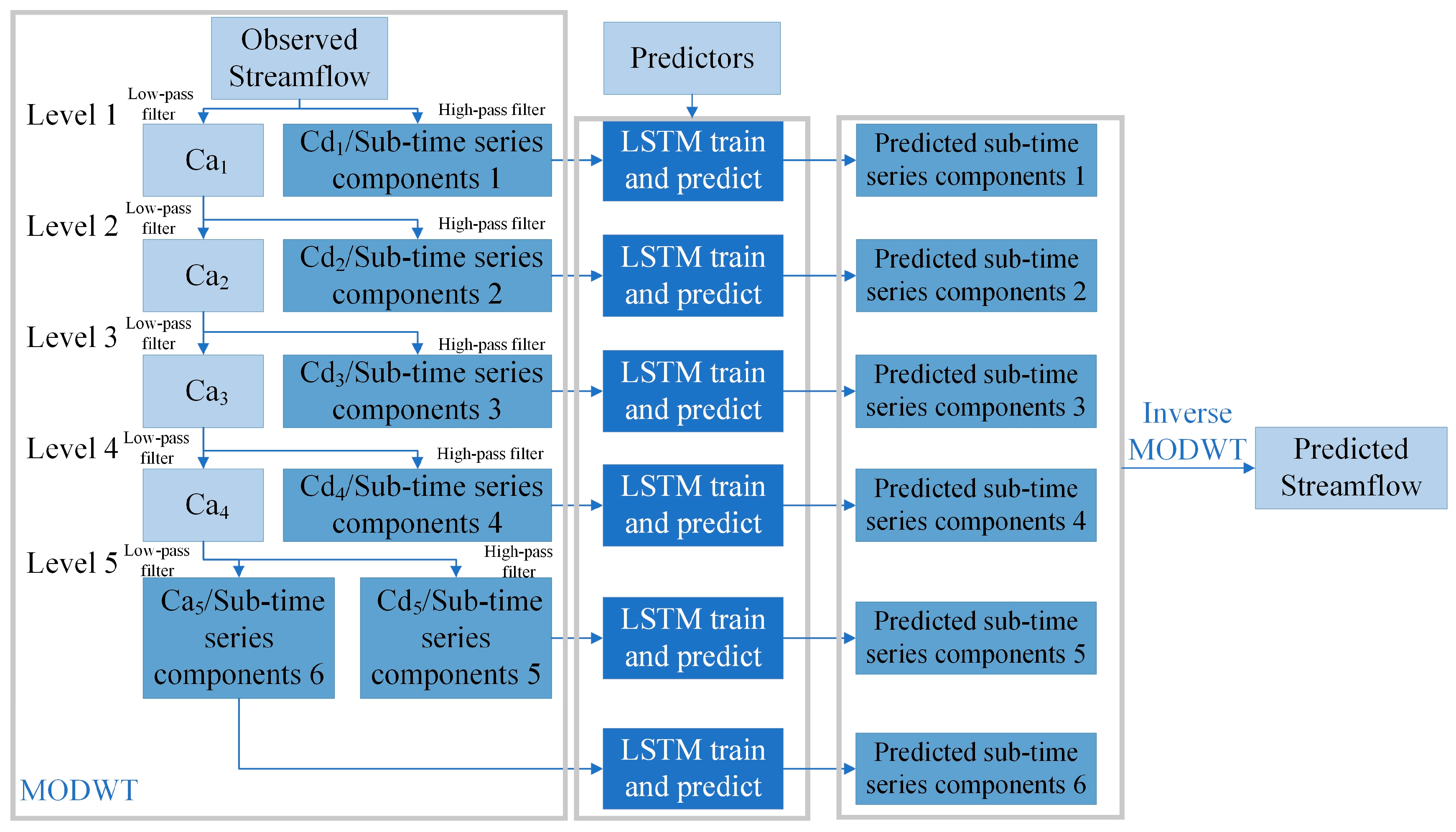
3.1. SSA-MODWT-LSTM Model

Many previous studies [33,34,35,36] using the decomposition method for ML prediction first decomposed the runoff time series into a sub-time series and then split these sub-time series into a train period and a test period, achieving better accuracy for prediction in the test period. Because the decomposition process in these studies uses the whole time series to decompose, that means the sub-time series of the train period contain the information from the test period if the data in the train and test period are decomposed together, which is called information leaking. In this study, we avoided this problem of information leaking by first dividing the train period and the test period, and, then, we decomposed the train set and the test set separately, which means that the decomposition of the train period and test period is independent. Additionally, the inconsistency in the lengths of the train set and test set results in a different number of sub-time series decomposed by the traditional EMD method, which poses difficulty for simulation and prediction. To address this issue, MODWT was used in this study because it can appoint the number of sub-time series to be composed. MODWT is an improved approach to DWT by avoiding down-sampling during data decomposition. In this study, the runoff sequence was decomposed at five levels using MODWT and sym4 mother wavelet to obtain five detailed coefficient sequences and one approximate coefficient sequence because the highest level of MODWT decomposition supported by Matlab R2024b is 5 levels. The research conducted by Salah Difi et al. [37] indicates that the sym4 mother wavelet performs better in the decomposition of runoff. These six sequences are considered sub-sequences and then were trained and predicted using the LSTM. The Kolmogorov–Smirnov test [38] shows that MODWT decomposition for the training period is representative and can be used to predict the runoff in the prediction period.

Numerous studies found that discrete wavelet decomposition outperforms other decomposition algorithms in the field of runoff simulation and prediction [33,35]. DWT is a multi-resolution analysis (MRA) technique that decomposes a signal into an approximation coefficient and multiple detailed coefficients [39]. One of the two problems with DWT is that we have to process the data length into an integer power of two. Another problem is that each decomposition halves the length of the data, which brings difficulties in its application. The MODWT solves these two problems by using circular convolution to process data and avoiding down-sampling, making it more suitable for modern computing devices. In addition to this, the two improvements mentioned above also facilitate the simulation and prediction.

LSTM is a type of recurrent neural network (RNN) architecture designed to effectively capture and learn long-term dependencies in sequential data [40]. In contrast to the neurons of traditional RNN models, the neurons in LSTM include three types of gates, enabling superior performance in the prediction of long sequence data by LSTM compared to RNN. The SSA is an intelligent optimization algorithm that derives its principles from the foraging and anti-predatory behavior of sparrows [41], which searches the solution space in a distributed, parallel manner to find the optimal or near-optimal solution to an optimization problem.

SHAP is a generalized method for interpreting machine learning models, which is improved on SHAPley values [42]. In contrast to the traditional method such as mutual information (MI) for determining the importance of input, SHAP demonstrates the impact of different input on the prediction results. It computes the average of the marginal contributions of a input variable across all scenarios, i.e., the SHAP value of the predictor [43]. Assuming that the i-th scenario is $x_i$, the j-th predictor of the i-th scenario is $x_{ij}$, the predicted value of the model for this sample is $y_i$, and the mean of the sample’s target variable is $y_{base}$, the relationship between the contribution value and the predicted value is

$$y_i=y_{base}+f\left(x_{i1}\right)+f\left(x_{i2}\right)+\cdots +f\left(x_{ik}\right),$$

(1)

In Equation (1), $f\left(x_{i1}\right)$ is the effect of the first input variable in the i-th scenario to the final predicted value $y_i$. $f\left(x_{i1}\right)$ > 0 represents that the input results cause an increase in the predicted value, and the opposite indicates a negative effect. It is worth noting that Equation S1 is only one of countless input sequences, and the SHAP optimized the algorithm to ensure its accuracy; therefore, it is possible to quickly calculate the marginal contribution and SHAP value of predictors across all input sequences [44]. SHAP can also calculate the effect of individual predictors on individual predicted values.

XGBoost is an efficient and scalable supervised machine learning algorithm based on gradient boosting [45]. It has been used in a wide range of industries due to its excellent performance, robustness, and outstanding efficiency. XGBoost consists of a set of classification and regression trees (CARTs) [46], each of which performs gradient boosting based on the prediction of the previous tree [47]. The final predicted value ${\widehat{y}}_i$ is the sum of all tree calculations:

$${\widehat{y}}_i=\varphi \left({\chi }_i\right)={{\displaystyle \sum }}_{k=1}^K{f}_k\left(x_i\right),f_k\in F,$$

(2)

$$F=\left\{f\left(x\right)=w_{q\left(x\right)}\right\}\left(q:R^m\to T,w\in R^T\right)$$

(3)

where f is a function in the function space F, F represents the set of all possible CARTs, K denotes the number of trees, q denotes that each tree maps an example to the corresponding leaf index, T is the number of leaves in the tree, and w is the weight of leaf. After substitution, the final predicted value can also be expressed as follows:

$${\widehat{y}}_i^t={\widehat{y}}_i^{t-1}+f_t\left(x_i\right)$$

(4)

Therefore, it is important to try to optimize the reduced objective function into the form of Equation (5):

$$J\left(f_t\right)={{\displaystyle \sum }}_{i=1}^{n}L\left(y_{i,}{\widehat{y}}_i^{t-1}+f_t\left(x_i\right)\right)+\mathsf{\Omega }\left(f_t\right)$$

(5)

where $L\left(y_{i,}{\widehat{y}}_i^{t-1}+f_t\left(x_i\right)\right)$ is the loss function, and $\mathsf{\Omega }\left(f_t\right)$ denotes the complexity of the tree model. Equation (6) [45] is the calculation of complexity, which is also known as regularization:

$$\Omega \left(f_t\right)=\gamma ·T_t+\lambda {\displaystyle \frac{1}{2}}{{\displaystyle \sum }}_{j=1}^T{w}_j^2$$

(6)

In this study, we used the method proposed by Chen and Guestrin [45], which runs the XGBoost in a parallel manner, allowing the full use of multi-core CPUs during training and achieving higher computational speeds.

In this study, we propose a framework combining decomposition method with ML (Figure 3). We decomposed the observed runoff sequence into six sub-sequences using the Maximal Overlap Discrete Wavelet Transform (MODWT) method. Then, the predictors were used as input into the Long Short-Term Memory (LSTM) model to train and predict these six sub-sequences, respectively, and we used the wavelet inverse transformation of the six sub-sequences to obtain the predicted runoff (Figure 4). Three hyperparameters of the LSTM were determined: the number of nodes in the hidden layer, the maximum number of training epochs, and the learning rate. These parameters were optimized using the Sparrow Search Algorithm (SSA) within the specified ranges: 50–300 for the number of nodes, 10–300 for the maximum training epochs, and 0.001–0.01 for the learning rate. To better accommodate the runoff during periods of high flow, the RMSE loss function was improved during the training process. Specifically, the weights for local maximum data point together with one point before and after it, were adjusted to a parameter w, which was also optimized using the SSA within the range of 2–20.

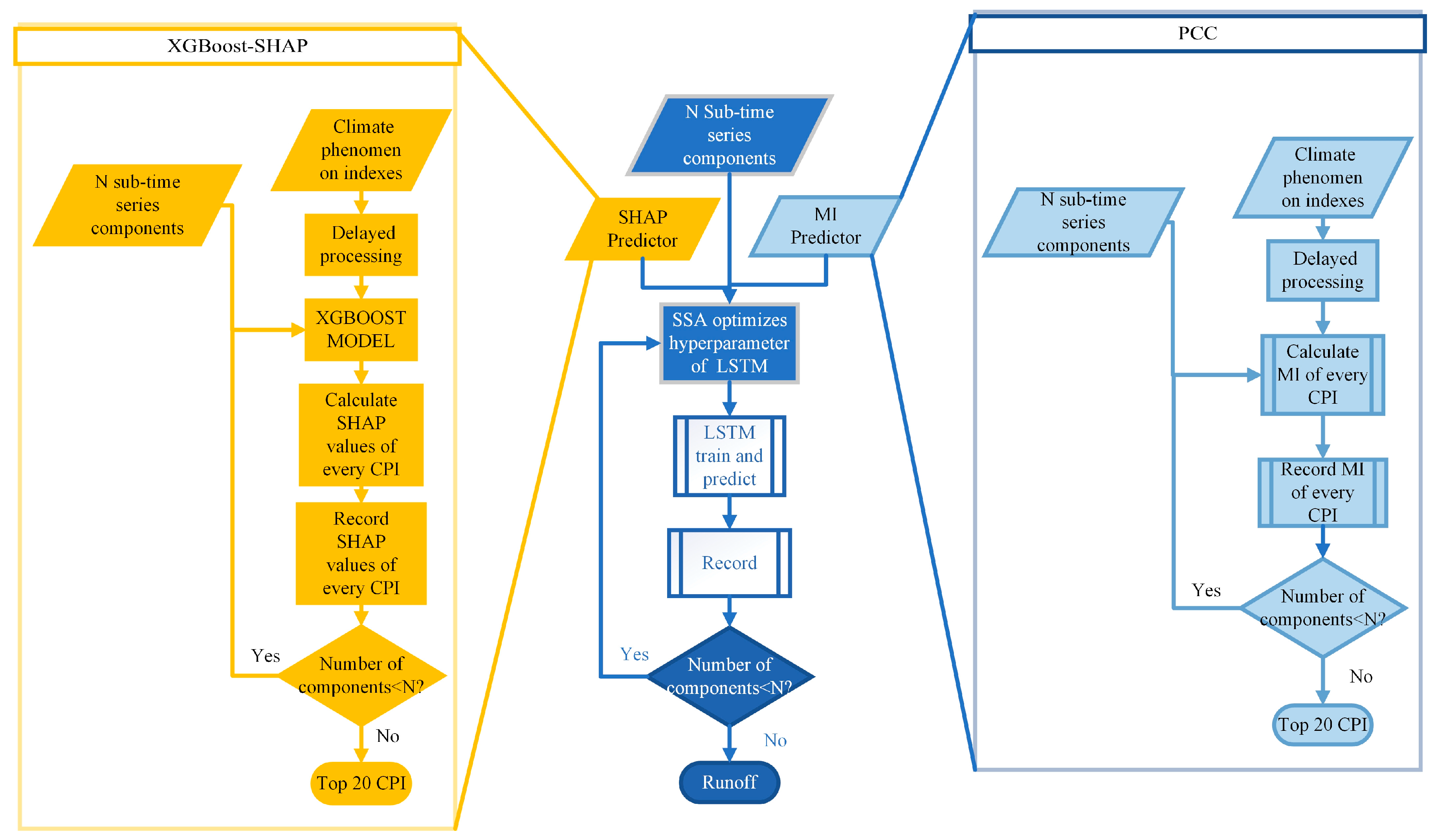
3.2. Selection of Predictors

In this study, we used XGBOOST-SHAP to perform predictor selection. SHapley Additive Explanations (SHAP) was used to find the climate indices that have significant impact on the XGBoost, and these indices were selected as suitable predictors that constitute the input of LSTM. We also analyzed the physical meaning of the selected predictors. As shown in Figure 3, when setting up the XGBoost model, we used the indices in a time window from the current month to prior twelve months as inputs of XGBoost. XGBoost used all the indices to simulate each sub-time series component and then calculated the SHAP values for each index at various leading times. Finally, the SHAP values for each indices were summarized. We selected the predictors with SHAP values from high to low as inputs and also incorporated the historical runoff data. And the physical interpretation of the predictors selected by the XGBoost-SHAP was analyzed to verify the reasonability of XGBoost-SHAP for predictor selection (see Section 5).

3.3. Model Setup and Method of Model Performance Evaluation

We compared the performance of the SSA-MODWT-LSTM model and MODWT- LSTM model without the parameter optimization of the SSA. We also compared the model with predictor selection using XGBoost-SHAP and mutual information (MI), and the model without predictor selection was also added to the comparison. If the leading time for the runoff forecast was one month, we used data from the current month to 12 months ago to predict runoff in the next month. Then, correlation coefficients were calculated between each factor from last month to twelve months ago and the runoff data of this month. We further compared the performance of MODWT-LSTM with the LSTM, which is not combined with MODWT. In addition, we compared the performance of the SHAP-SSA-MODWT-LSTM and MI-SSA-MODWT-LSTM models for different leading times when the leading time for the runoff forecast is extended for more than one month. All the model setups are summarized in

Table 1. Design of model setups.

Model Setting	Model with MODWT	Model Without MODWT
MODWT with SSA	SHAP-SSA-MODWT-LSTM	SHAP-SSA-LSTM
	MI-SSA-MODWT-LSTM	MI-SSA-LSTM
MODWT without SSA	SHAP-MODWT-LSTM	SHAP-LSTM
	MI-MODWT-LSTM	MI-LSTM

Note: SHAP represents SHapley Additive Explanations for predictor selection, MI represents Pearson’s correlation coefficient used for predictor selection, the SSA represents a model that includes Sparrow Search Algorithm, and MODWT represents a model using Maximal Overlap Discrete Wavelet Transform.

.

Several quantitative metrics were chosen to evaluate the accuracy of the model, including the Nash–Sutcliffe efficiency (NSE) coefficient [48], Pearson’s correlation coefficient (R), bias [49], root mean square error (RMSE), and mean absolute relative error (MARE). These metrics are calculated as follows:

$$NSE=1-{\displaystyle \frac{{{\displaystyle \sum }}_{i=1}^N{\left(Q_i^s-Q_i^o\right)}^2}{{{\displaystyle \sum }}_{i=1}^N{\left(Q_i^s-{\overline{Q}}^0\right)}^2}}$$

(7)

$$R={\displaystyle \frac{{{\displaystyle \sum }}_{i=1}^N\left(Q_i^s-{\overline{Q}}^o\right)\left(Q_i^s-{\overline{Q}}^s\right)}{\sqrt{{{\displaystyle \sum }}_{i=1}^N{\left(Q_i^s-{\overline{Q}}_i^o\right)}^2{{\displaystyle \sum }}_{i=1}^N{\left(Q_i^s-{\overline{Q}}_i^s\right)}^2}}}\times 100\%$$

(8)

$$Bias={\displaystyle \frac{{{\displaystyle \sum }}_{i=1}^N{\left(Q_i^s-Q_i^o\right)}^2}{{{\displaystyle \sum }}_{i=1}^N{Q}_i^o}}\times 100\%$$

(9)

$$RMSE=\sqrt{{\displaystyle \frac{1}{N}}{{\displaystyle \sum }}_{i=1}^N{w}_i{\left(Q_i^s-Q_i^o\right)}^2}$$

(10)

$$MARE={\displaystyle \frac{1}{N}}{{\displaystyle \sum }}_{i=1}^N\left|{\displaystyle \frac{Q_i^o-Q_i^s}{Q_i^o}}\right|$$

(11)

where N represents the number of the time steps, $Q_i^s$ and $Q_i^o$ are the predicted and observed runoff sequences, and ${\overline{Q}}^s$ and ${\overline{Q}}^o$ are the averages of the simulated and observed runoff. $w_i$ is the weight of couples $Q_i^o$ and $Q_i^s$, among which the weights of the local maximum point and its two neighboring points are optimized by the SSA.

4. Results

4.1. The Runoff Components Decomposed by MODWT

In this study, we use MODWT to apply sym4 mother wavelets to decompose the runoff sequences at the two hydrology stations into five sets of detailed coefficients and one set of approximate coefficients. The decomposition of streamflow at Tobolsk station is shown in Figure 5. The results shown in

Table 2. Characteristics of each subsequence. Skew, Stdev, Var, and Entropy, respectively, stand for skewness, standard deviation, variance, and sample entropy.

IMFs	Period	Mean	Max	Min	Skewn	Stdev	Var	Entropy
IMF1	Train Period	0.00	2437.59	−2579.58	0.01	558.26	311,658.00	2.38
IMF1	Test Period	0.00	1621.74	−1450.39	0.27	490.20	240,297.30	2.81
IMF2	Train Period	0.00	2582.46	−3579.18	−0.61	957.03	915,909.50	2.83
IMF2	Test Period	0.00	2014.88	−3112.34	−0.62	979.14	958,724.40	3.00
IMF3	Train Period	0.00	2729.02	−3023.41	−0.15	1263.89	1,597,407.00	3.22
IMF3	Test Period	0.00	2700.79	−3197.62	−0.25	1240.70	1,539,334.00	3.12
IMF4	Train Period	0.00	994.08	−1071.44	−0.37	408.83	167,144.70	3.12
IMF4	Test Period	0.00	745.83	−1425.88	−0.70	444.49	197,569.10	3.11
IMF5	Train Period	0.00	549.76	−671.03	−0.19	242.26	58,689.93	3.15
IMF5	Test Period	0.00	505.60	−706.62	−0.54	257.94	66,534.04	3.14
IMF6	Train Period	2033.11	3082.00	1249.65	0.32	410.58	168,575.20	3.23
IMF6	Test Period	2253.28	2869.28	1645.44	−0.10	305.10	93,085.53	3.15

indicate that the patterns of the decomposed sets during the training period and the test period did not show significant differences, which illustrates the robustness of the MODWT. This suggests that the model calibrated based on the decomposed runoff in the training period is reliable to be applied to predict the runoff in the test period.

Wavelet analysis was also used for periodicity analysis. When the real part value of the wavelet coefficient is positive, it represents the period of high flow; and, when it is negative, it represents the period of low flow. Wavelet analysis of streamflow at the Tobolsk and Omsk stations is shown in Figure 5 and Figure 6. Figure 6a and Figure 7a illustrate that the runoff change at the Omsk station and Tobolsk station from 1951 to 2012 shows characteristics across multiple time scales. The primary oscillatory cycle during this period at Omsk and Tobolsk are approximately 23 and 25 years, although its effect is diminishing over time. The changes in the scale of 10–17 years are more stable after the 1970s, and the cycle of 8 years is quite stable after 1985 at Omsk. The cycle of 10 to 17 years remained stable until the 1990s at Tobolsk. Figure 6b demonstrates three distinct peaks in the streamflow at the Omsk station, corresponding to time scales of approximately 8, 14, and 23 years. The highest peak is at the 8-year time scale, indicating the strongest oscillation at this cycle. The second primary cycle is about 14 years, the third primary cycle is about 23 years, and Figure 7b shows that the largest major cycles at Tobolsk are about 7, 14, and 25 years.

At the two stations, the test set did not include all the cycles due to sequence length, which may influence our results. However, increasing the length of the test set could adversely affect the training, so we did not shorten the length of the training set to increase the length of the test set. We have also tested the model sensitivity for the length of the test period. The NSE values of the proposed model in the test period at Tobolsk with the training set proportions of 0.6 and 0.8 were 0.843 and 0.877, respectively, which are lower than that for the training set proportion of 0.7. It should be noticed that the test set includes the first and second primary cycles, which may explain the similar pattern of the decomposed runoff series between the training and test periods.

4.2. Performance of the SSA-MODWT-LSTM Model

4.2.1. Evaluation of SSA and MODWT

Table 3. Statistics of the metrics for different model performances with one month of leading time.

Stations	Models	NSE	R	Bias (%)	MARE (%)
Omsk	SHAP-SSA-MODWT-LSTM	0.851	0.927	−0.640	14.743
	SHAP-MODWT-LSTM	0.708	0.852	−1.576	21.173
	SHAP-SSA-LSTM	0.725	0.861	−2.086	18.429
	SHAP-LSTM	0.682	0.823	−2.301	23.361
	MI-SSA-MODWT-LSTM	0.793	0.907	−2.074	18.034
	MI-MODWT-LSTM	0.761	0.881	−1.789	20.121
	MI-SSA-LSTM	0.738	0.870	3.094	15.410
	MI-LSTM	0.703	0.812	−3.938	19.549
Tobolsk	SHAP-SSA-MODWT-LSTM	0.941	0.971	−1.732	16.977
	SHAP-MODWT-LSTM	0.794	0.906	−2.870	28.510
	SHAP-SSA-LSTM	0.757	0.884	−7.325	22.310
	SHAP-LSTM	0.702	0.811	−9.276	26.375
	MI-SSA-MODWT-LSTM	0.813	0.916	−12.760	25.306
	MI-MODWT-LSTM	0.787	0.907	−13.697	25.532
	MI-SSA-LSTM	0.797	0.897	−14.302	16.818
	MI-LSTM	0.721	0.883	−17.203	18.212

displays the performance of various models with a leading time of one month. Models optimized with the SSA consistently demonstrate improved performance compared to those without the SSA. For instance, at both the Omsk and Tobolsk stations, models incorporating the SSA show higher NSE and R values together with reductions in bias and MARE. This underscores the effectiveness of the SSA in enhancing model performance.

Similarly, the benefits of incorporating MODWT are evident. At both of the two stations, MODWT-based models outperform their counterparts without MODWT, with notable improvements in the NSE and R, along with reductions in bias and MARE. For example, at the Tobolsk station, the SHAP-SSA-MODWT-LSTM model demonstrated substantial improvements over the SHAP-SSA-LSTM model, with the NSE increasing by 24.3% (from 0.757 to 0.941), absolute bias reduced by 76.3% (from −7.325% to −1.732%), and MARE decreasing by 23.9% (from 22.310% to 16.977%). These results emphasize the advantages of combining MODWT with LSTM, which evidently enhanced the predictive capabilities of the models.

4.2.2. Comparison of the Performance Between SHAP and MI

Figure 8 and Table 3 illustrate the performance of the MI-MODWT-LSTM, SHAP-MODWT-LSTM, and MODWT-LSTM models for a leading time of one month. At the Omsk station, the SHAP-MODWT-LSTM model outperforms both the MODWT-LSTM and MI-MODWT-LSTM models across all four evaluation criteria. Similarly, at the Tobolsk station, the SHAP-MODWT-LSTM model demonstrates superior performance in all evaluation metrics compared to the other models. In comparison to the MI-MODWT-LSTM model, the SHAP-MODWT-LSTM model exhibited an increase in the NSE by 0.128 and an increase in R by 0.055, and also a decrease in the absolute value of bias by 11.028% and a decrease in MARE by 8.329%. It was observed that the month with the highest flow is May at Omsk and June at Tobolsk. The SHAP-MODWT-LSTM model shows good agreement with observed values, particularly for peak flows. Compared with the MI-MODWT-LSTM method, the MARE of Omsk and Tobolsk have decreased by 1.06% and 8.45%, respectively. Figure 9 and

Table 4. Comparison of the performance with a leading time of one month for MI-MODWT-LSTM, SHAP-MODWT-LSTM, and MODWT-LSTM in May at the Omsk station and in June at the Tobolsk station.

Stations	Models	NSE	R	Bias (%)	MARE (%)
Omsk	MI-SSA-MODWT-LSTM	0.600	0.742	−2.353	7.627
	SHAP-SSA-MODWT-LSTM	0.664	0.847	−2.276	5.569
	SSA-MODWT-LSTM	0.374	0.706	−2.998	7.752
Tobolsk	MI-SSA-MODWT-LSTM	0.623	0.725	−4.453	18.473
	SHAP-SSA-MODWT-LSTM	0.846	0.946	−0.847	10.015
	SSA-MODWT-LSTM	0.457	0.647	−7.936	17.465

present the predicted streamflow for the months with the highest flow in each year during the test period, further confirming the better performance of SHAP-MODWT-LSTM.

These results show that XGBoost-SHAP leads to a more reasonable selection of predictors at both the Tobolsk and Omsk stations compared to MI and models with no predictor identification algorithms. The MI method outperformed the model with no identification algorithm for predictors. This means that the XGBoost-SHAP is effective in screening and identifying the key climatic factors affecting runoff and improving model performance in large watersheds such as the Irtysh River.

4.2.3. Model Performance at Different Leading Time

Figure 10 demonstrates that, for peak runoff months at the two hydrological stations, the performance of SHAP-MODWT-LSTM generally declines, with the MARE and RMSE increasing as the lead time extends from one to seven months. The reduction in performance at the Tobolsk station was more moderate than that at the Omsk station. This also shows that, in months with peak runoff, the performance of MI-MODWT-LSTM at the Omsk and Tobolsk stations exhibits a fluctuating downward trend, with the RMSE and MARE evidently increasing as the lead time extends. This suggests that the longer the leading time, the worse the results of the predictions. However, the decline of performance when lead time increases by using the SHAP method is slower than using the MI method as lead time increases from 1 to 4 months. This illustrates the advantage for using the SHAP method. With the extension of the forecast period, the correlation between the historical predictors and the forecast runoff will decline, resulting in the deterioration of the model’s performance.

4.3. Predictor Identified by XGBoost-SHAP Model in Data Limited Area

The top twenty influential factors identified by XGBoost-SHAP at the Tobolsk station for simulations with a leading time of one month are shown in Figure 11. Some climatic indices, such as the North African Subtropical High Ridge Position, have been demonstrated to influence precipitation and runoff in the study area in previous studies [50]. However, the individual effects of other climatic phenomena indices (CPIs) on precipitation and runoff in Central Asia have yet to be elucidated individually. A more detailed and in-depth analysis of these predictors is presented in Section 5.2.

5. Discussion

5.1. Performance of the SHAP-SSA-MODWT-LSTM Model

The XGBoost can identify nonlinear influences of predictors on the runoff to enhance the performance of model prediction. However, XGBoost is designed to processes data in a static manner, and it cannot identify the chronological order [45], even if the predictors of delayed series are constructed manually to enable XGBoost the ability to predict time series data [51]. It is still impossible to dynamically model long-term dependencies like LSTM [52]. Therefore, the use of XGBoost to identify long-term influences of predictor on runoff is still debatable.

In this study, we developed an ML model in a limited field meteorological data area without relying on local observed meteorological data and obtained acceptable accuracy in runoff prediction using large-scale indices. This indicates the advantages of a ML-based runoff prediction method in data-scarce basins combining the predictor selection method, as it can utilize easily accessible large-scale factors to obtain accurately predicted runoff by exploring the nonlinear relationship between runoff and large scale predictors. However, it still has limitations, and the accuracy of the method developed in this study may decrease as the watershed area declines. For example, the accuracy at the Omsk station is lower than that at the Tobolsk station, which has a larger drainage watershed. The watershed area downstream the Tobolsk station is large, and the influencing factors of streamflow are complex. Therefore, the SHAP-MODWT-LSTM can well recognize the nonlinear influencing factors, and, thus, the results are better than the MI-MODWT-LSTM. The SHAP value quantitatively indicates the predictor’s influence on the results. When it is >0, it tends to show that the predictor causes the results to be larger and vice versa. The simple summing approach that we used in our study will result in the sum of SHAP values to converge to zero in some specific cases, and this will not accurately reflect the impact of the predictor on the results. On the other hand, this study does not give weights to the SHAP values according to the contribution of each runoff component to the runoff. However, the XGBoost-SHAP method used in this study still showed better performance than MI in most scenarios.

Modal decomposition methods like EMD and VMD may cause information leakage by decomposing runoff from both the training and test periods together, leading to artificially improved model performance. For runoff sequences in this study, we found that the results of the decomposition in the training period alone are not representative for that in the test period. However, the MODWT used in this study shows reliability for runoff decomposition. The functions developed in the training period for runoff decomposition are also representative in the test period. The comparison of different runoff decompositions need to be more deeply studied in the future.

5.2. Interpretation of the Predictor Identified by XGBoost-SHAP Model

In Central Asia, the sources of water vapor exhibit great complexity and can be categorized into eastern and western regions based on the seasonality of precipitation, with the boundary approximately at 72.5° N. Yang et al. [53] found that the source of water vapor for Central Asia is mainly in Western Asia and Europe through simulations by the Hysplit model. In winter, the water vapor path in Western Central Asia extends southward as far as Northern Africa and the Arabian Sea at about 10°N, north to the Arctic, and east to Western Siberia [54]. The above sources of water vapor explain the selected predictors such as the North African–North Atlantic–North American Subtropical High Ridge Position Index, the Northern Hemisphere Polar Vortex Intensity Index [55], the Indian Ocean Warm Pool Area Index, and Strength Index [56]. In summer, the path of water vapor extends eastward as far as Eastern Central Siberia, south to about 20° N, and westward to Northern America. Therefore, the Asia Polar Vortex Intensity Index, the North American Subtropical High Ridge Position Index, and the North American Polar Vortex Intensity Index are identified here. Botsyun et al. [57] discovered that rainfall in Central Asia is strongly connected to the East Asian summer winds, the Indian summer winds, and the westerly rapids. That is why the East Asian Trough Strength Index and the Tibet Plateau Region 1 Index [54] are identified by XGBoost-SHAP.

Some of the predictors selected by XGBoost-SHAP do not have high correlation coefficients with observed streamflow, which shows that the streamflow in this basin is affected by many nonlinear predictors, and these can be effectually identified by XGBoost-SHAP.

6. Conclusions

In this study, we propose a model combining the runoff decomposition by MODWT with LSTM, and a method of XGBoost-SHAP is developed for predictor selection as model input. The model and method that we developed demonstrated good performance in monthly runoff forecast at two stations in the Irtysh River Basin. The main conclusions are drawn as follows:

(1) MODWT shows a robustness for runoff decomposition between the training period and test period. The MODWT-LSTM model that we proposed can effectively improve the accuracy of monthly runoff forecast compared with the sole LSTM model. Using the SSA for parameter optimization can also enhance the model performance.

(2) The XGBoost-SHAP method achieves superior accuracy in forecasting runoff at both the Omsk and Tobolsk stations compared to the traditional MI method for predictor selection. This is because that XGBoost-SHAP effectively identifies key nonlinear factors associated with runoff, and the recognized climate factors are plausible in terms of physical mechanisms.

(3) The models and methods that we developed in this study have potential for application in hydrological forecast in regions with poorly field observed meteorological data.

References

1. Liang, W.; Chen, Y.; Fang, G.; Kaldybayev, A. Machine Learning Method Is an Alternative for the Hydrological Model in an Alpine Catchment in the Tianshan Region, Central Asia. J. Hydrol. Reg. Stud. 2023, 49, 101492. [Google Scholar] [CrossRef]
2. Chen, S.; Ren, M.; Sun, W. Combining Two-Stage Decomposition Based Machine Learning Methods for Annual Runoff Forecasting. J. Hydrol. 2021, 603, 126945. [Google Scholar] [CrossRef]
3. Yang, S.; Yang, D.; Chen, J.; Santisirisomboon, J.; Lu, W.; Zhao, B. A Physical Process and Machine Learning Combined Hydrological Model for Daily Streamflow Simulations of Large Watersheds with Limited Observation Data. J. Hydrol. 2020, 590, 125206. [Google Scholar] [CrossRef]
4. Jougla, R.; Leconte, R. Short-Term Hydrological Forecast Using Artificial Neural Network Models with Different Combinations and Spatial Representations of Hydrometeorological Inputs. Water 2022, 14, 552. [Google Scholar] [CrossRef]
5. Wang, L.; Li, X.; Ma, C.; Bai, Y. Improving the Prediction Accuracy of Monthly Streamflow Using a Data-Driven Model Based on a Double-Processing Strategy. J. Hydrol. 2019, 573, 733–745. [Google Scholar] [CrossRef]
6. Tegegne, G.; Park, D.K.; Kim, Y.O. Comparison of Hydrological Models for the Assessment of Water Resources in a Data-Scarce Region, the Upper Blue Nile River Basin. J. Hydrol. Reg. Stud. 2017, 14, 49–66. [Google Scholar] [CrossRef]
7. Scaling Point-Scale (Pedo)Transfer Functions to Seamless Large-Domain Parameter Estimates for High-Resolution Distributed Hydrologic Modeling: An Example for the Rhine River-Imhoff-2020-Water Resources Research-Wiley Online Library. Available online: https://agupubs.onlinelibrary.wiley.com/doi/10.1029/2019WR026807 (accessed on 15 April 2025).
8. Li, K.; Wang, Y.; Li, X.; Yuan, Z.; Xu, J. Simulation Effect Evaluation of Single-Outlet and Multi-Outlet Calibration of Soil and Water Assessment Tool Model Driven by Climate Forecast System Reanalysis Data and Ground-Based Meteorological Station Data—A Case Study in a Yellow River Source. Water Supply 2020, 21, 1061–1071. [Google Scholar] [CrossRef]
9. Gu, P.; Wang, G.; Liu, G.; Wu, Y.; Liu, H.; Jiang, X.; Liu, T. Evaluation of Multisource Precipitation Input for Hydrological Modeling in an Alpine Basin: A Case Study from the Yellow River Source Region (China). Hydrol. Res. 2022, 53, 314–335. [Google Scholar] [CrossRef]
10. Li, C.; Cai, Y.; Li, Z.; Zhang, Q.; Sun, L.; Li, X.; Zhou, P. Hydrological Response to Climate and Land Use Changes in the Dry–Warm Valley of the Upper Yangtze River. Engineering 2022, 19, 24–39. [Google Scholar] [CrossRef]
11. Barbetta, S.; Sahoo, B.; Bonaccorsi, B.; Nanda, T.; Chatterjee, C.; Moramarco, T.; Todini, E. Addressing Effective Real-Time Forecasting Inflows to Dams through Predictive Uncertainty Estimate. J. Hydrol. 2023, 620, 129512. [Google Scholar] [CrossRef]
12. Xi, Y.; Peng, S.; Ducharne, A.; Ciais, P.; Gumbricht, T.; Jimenez, C.; Poulter, B.; Prigent, C.; Qiu, C.; Saunois, M.; et al. Gridded Maps of Wetlands Dynamics over Mid-Low Latitudes for 1980–2020 Based on TOPMODEL. Sci. Data 2022, 9, 347. [Google Scholar] [CrossRef]
13. Box, G.E.P.; Jenkins, G.M.; Reinsel, G.C.; Ljung, G.M. Time Series Analysis: Forecasting and Control; John Wiley & Sons: Hoboken, NJ, USA, 2015; ISBN 978-1-118-67492-5. [Google Scholar]
14. Kwon, H.-H.; Brown, C.; Xu, K.; Lall, U. Seasonal and Annual Maximum Streamflow Forecasting Using Climate Information: Application to the Three Gorges Dam in the Yangtze River Basin, China. Hydrol. Sci. J. 2009, 54, 582–595. [Google Scholar] [CrossRef]
15. Panahi, F.; Ehteram, M.; Ahmed, A.N.; Huang, Y.F.; Mosavi, A.; El-Shafie, A. Streamflow Prediction with Large Climate Indices Using Several Hybrid Multilayer Perceptrons and Copula Bayesian Model Averaging. Ecol. Indic. 2021, 133, 108285. [Google Scholar] [CrossRef]
16. Aghaabbasi, M.; Chalermpong, S. Machine Learning Techniques for Evaluating the Nonlinear Link between Built-Environment Characteristics and Travel Behaviors: A Systematic Review. Travel Behav. Soc. 2023, 33, 100640. [Google Scholar] [CrossRef]
17. Wang, S.; Peng, H.; Hu, Q.; Jiang, M. Analysis of Runoff Generation Driving Factors Based on Hydrological Model and Interpretable Machine Learning Method. J. Hydrol. Reg. Stud. 2022, 42, 101139. [Google Scholar] [CrossRef]
18. Zhao, X.; Lv, H.; Lv, S.; Sang, Y.; Wei, Y.; Zhu, X. Enhancing Robustness of Monthly Streamflow Forecasting Model Using Gated Recurrent Unit Based on Improved Grey Wolf Optimizer. J. Hydrol. 2021, 601, 126607. [Google Scholar] [CrossRef]
19. Xu, D.; Liao, A.; Wang, W.; Tian, W.; Zang, H. Improved Monthly Runoff Time Series Prediction Using the CABES-LSTM Mixture Model Based on CEEMDAN-VMD Decomposition. J. Hydroinform. 2023, 26, 255–283. [Google Scholar] [CrossRef]
20. Zhang, X.; Wang, R.; Wang, W.; Zheng, Q.; Ma, R.; Tang, R.; Wang, Y. Runoff Prediction Using Combined Machine Learning Models and Signal Decomposition. J. Water Clim. Change 2024, 16, 230–247. [Google Scholar] [CrossRef]
21. Cai, X.; Li, D. M-EDEM: A MNN-Based Empirical Decomposition Ensemble Method for Improved Time Series Forecasting. Knowl.-Based Syst. 2024, 283, 111157. [Google Scholar] [CrossRef]
22. Ji, Y.; Dong, H.-T.; Xing, Z.-X.; Sun, M.-X.; Fu, Q.; Liu, D. Application of the Decomposition-Prediction-Reconstruction Framework to Medium- and Long-Term Runoff Forecasting. Water Supply 2020, 21, 696–709. [Google Scholar] [CrossRef]
23. Wrzesiński, D.; Sobkowiak, L.; Mares, I.; Dobrica, V.; Mares, C. Variability of River Runoff in Poland and Its Connection to Solar Variability. Atmosphere 2023, 14, 1184. [Google Scholar] [CrossRef]
24. Russell, G.L.; Miller, J.R. Global River Runoff Calculated from a Global Atmospheric General Circulation Model. J. Hydrol. 1990, 117, 241–254. [Google Scholar] [CrossRef]
25. Nguyen, T.-T.-H.; Li, M.-H.; Vu, T.M.; Chen, P.-Y. Multiple Drought Indices and Their Teleconnections with ENSO in Various Spatiotemporal Scales over the Mekong River Basin. Sci. Total Environ. 2023, 854, 158589. [Google Scholar] [CrossRef]
26. Tosunoglu, F.; Kahya, E.; Ghorbani, M.A. Spatial and Temporal Linkages between Large-Scale Atmospheric Oscillations and Hydrologic Drought Indices in Turkey. In Integrated Drought Management, Volume 2; CRC Press: Boca Raton, FL, USA, 2023; ISBN 978-1-003-27654-8. [Google Scholar]
27. Chiew, F.H.S.; Piechota, T.C.; Dracup, J.A.; McMahon, T.A. El Nino/Southern Oscillation and Australian Rainfall, Streamflow and Drought: Links and Potential for Forecasting. J. Hydrol. 1998, 204, 138–149. [Google Scholar] [CrossRef]
28. Yongchao, L.; Yongjian, D.; Ersi, K.; Jishi, Z. The Relationship between ENSO Cycle and Temperature, Precipitation and Runoff in the Qilian Mountain Area. J. Geogr. Sci. 2003, 13, 293–298. [Google Scholar] [CrossRef]
29. Hernandez, D.; Mendoza, P.A.; Boisier, J.P.; Ricchetti, F. Hydrologic Sensitivities and ENSO Variability Across Hydrological Regimes in Central Chile (28°–41° S). Water Resour. Res. 2022, 58, e2021WR031860. [Google Scholar] [CrossRef]
30. Zhou, Y.; Mu, Z.; Peng, L.; Gao, R.; Yin, Z.; Tang, R. Mid-Term and Long-Term Hydrological Forecasting of Snowmelt Runoff in Western Tianshan Mountains Based on Mutual Information and Neural Network. J. Chang. River Sci. Res. Inst. 2018, 35, 17–21. [Google Scholar] [CrossRef]
31. Liao, S.; Liu, Z.; Liu, B.; Cheng, C.; Jin, X.; Zhao, Z. Multistep-Ahead Daily Inflow Forecasting Using the ERA-Interim Reanalysis Data Set Based on Gradient-Boosting Regression Trees. Hydrol. Earth Syst. Sci. 2020, 24, 2343–2363. [Google Scholar] [CrossRef]
32. BfG-GRDC Data Download. Available online: https://www.bafg.de/GRDC/EN/02_srvcs/21_tmsrs/210_prtl/prtl_node.html (accessed on 6 November 2023).
33. Yang, Y.; Li, W.; Liu, D. Monthly Runoff Prediction for Xijiang River via Gated Recurrent Unit, Discrete Wavelet Transform, and Variational Modal Decomposition. Water 2024, 16, 1552. [Google Scholar] [CrossRef]
34. Jamei, M.; Ali, M.; Malik, A.; Karbasi, M.; Rai, P.; Yaseen, Z.M. Development of a TVF-EMD-Based Multi-Decomposition Technique Integrated with Encoder-Decoder-Bidirectional-LSTM for Monthly Rainfall Forecasting. J. Hydrol. 2023, 617, 129105. [Google Scholar] [CrossRef]
35. Wang, W.; Du, Y.; Chau, K.; Xu, D.; Liu, C.; Ma, Q. An Ensemble Hybrid Forecasting Model for Annual Runoff Based on Sample Entropy, Secondary Decomposition, and Long Short-Term Memory Neural Network. Water Resour Manag. 2021, 35, 4695–4726. [Google Scholar] [CrossRef]
36. Huang, S.; Chang, J.; Huang, Q.; Chen, Y. Monthly Streamflow Prediction Using Modified EMD-Based Support Vector Machine. J. Hydrol. 2014, 511, 764–775. [Google Scholar] [CrossRef]
37. Difi, S.; Heddam, S.; Zerouali, B.; Kim, S.; Elmeddahi, Y.; Bailek, N.; Augusto Guimarães Santos, C.; Abida, H. Improved Daily Streamflow Forecasting for Semi-Arid Environments Using Hybrid Machine Learning and Multi-Scale Analysis Techniques. J. Hydroinform. 2024, 26, 3266–3286. [Google Scholar] [CrossRef]
38. Frank, M.J., Jr. The Kolmogorov-Smirnov Test for Goodness of Fit. J. Am. Stat. Assoc. 1951, 46, 68–78. [Google Scholar]
39. Patnaik, B.; Mishra, M.; Bansal, R.C.; Jena, R.K. MODWT-XGBoost Based Smart Energy Solution for Fault Detection and Classification in a Smart Microgrid. Appl. Energy 2021, 285, 116457. [Google Scholar] [CrossRef]
40. Sak, H.; Senior, A.; Beaufays, F. Long Short-Term Memory Based Recurrent Neural Network Architectures for Large Vocabulary Speech Recognition. arXiv 2014, arXiv:1402.1128. [Google Scholar]
41. Xue, J.; Shen, B. A Novel Swarm Intelligence Optimization Approach: Sparrow Search Algorithm. Syst. Sci. Control. Eng. 2020, 8, 22–34. [Google Scholar] [CrossRef]
42. The Shapley Value: Essays in Honor of Lloyd S., Shapley; Roth, A.E., Ed.; Cambridge University Press: Cambridge, UK, 1988; ISBN 978-0-521-36177-4. [Google Scholar]
43. Lundberg, S.M.; Lee, S.-I. A Unified Approach to Interpreting Model Predictions. In Proceedings of the 31st Conference on Neural Information Processing Systems (NIPS 2017), Long Beach, CA, USA, 4–9 December 2017; Curran Associates, Inc.: Red Hook, NY, USA, 2017; Volume 30. [Google Scholar]
44. Lundberg, S.M.; Erion, G.; Chen, H.; DeGrave, A.; Prutkin, J.M.; Nair, B.; Katz, R.; Himmelfarb, J.; Bansal, N.; Lee, S.-I. From Local Explanations to Global Understanding with Explainable AI for Trees. Nat. Mach. Intell. 2020, 2, 56–67. [Google Scholar] [CrossRef]
45. Chen, T.; Guestrin, C. XGBoost: A Scalable Tree Boosting System. In Proceedings of the 22nd ACM SIGKDD International Conference on Knowledge Discovery and Data Mining, San Francisco, CA, USA, 13–17 August 2016; pp. 785–794. [Google Scholar]
46. Breiman, L.; Friedman, J.; Olshen, R.A.; Stone, C.J. Classification and Regression Trees; Chapman and Hall/CRC: New York, NY, USA, 2017; ISBN 978-1-315-13947-0. [Google Scholar]
47. Friedman, J.H. Greedy Function Approximation: A Gradient Boosting Machine. Ann. Stat. 2001, 29, 1189–1232. [Google Scholar] [CrossRef]
48. Krause, P.; Boyle, D.P.; Bäse, F. Comparison of Different Efficiency Criteria for Hydrological Model Assessment. Adv. Geosci. 2005, 5, 89–97. [Google Scholar] [CrossRef]
49. Gupta, H.V.; Sorooshian, S.; Yapo, P.O. Status of Automatic Calibration for Hydrologic Models: Comparison with Multilevel Expert Calibration. J. Hydrol. Eng. 1999, 4, 135–143. [Google Scholar] [CrossRef]
50. Lu, X.; Zhao, Y. Relationships between North Africa Subtropical High and Summer Precipitation over Central Asia. Air Land Geogr. 2022, 45, 1050–1060. [Google Scholar] [CrossRef]
51. Makridakis, S.; Spiliotis, E.; Assimakopoulos, V. Statistical and Machine Learning Forecasting Methods: Concerns and Ways Forward. PLoS ONE 2018, 13, e0194889. [Google Scholar] [CrossRef]
52. Hewamalage, H.; Bergmeir, C.; Bandara, K. Recurrent Neural Networks for Time Series Forecasting: Current Status and Future Directions. Int. J. Forecast. 2021, 37, 388–427. [Google Scholar] [CrossRef]
53. Yang, H.; Xu, G.; Mao, H.; Wang, Y. Spatiotemporal Variation in Precipitation and Water Vapor Transport Over Central Asia in Winter and Summer Under Global Warming. Front. Earth Sci. 2020, 8, 297. [Google Scholar] [CrossRef]
54. Zhang, M.; Chen, Y.; Shen, Y.; Li, B. Tracking Climate Change in Central Asia through Temperature and Precipitation Extremes. J. Geogr. Sci. 2019, 29, 3–28. [Google Scholar] [CrossRef]
55. Wei, W.; Zou, S.; Duan, W.; Chen, Y.; Li, S.; Zhou, Y. Spatiotemporal Variability in Extreme Precipitation and Associated Large-Scale Climate Mechanisms in Central Asia from 1950 to 2019. J. Hydrol. 2023, 620, 129417. [Google Scholar] [CrossRef]
56. Huang, W.; Feng, S.; Chen, J.; Chen, F. Physical Mechanisms of Summer Precipitation Variations in the Tarim Basin in Northwestern China. J. Clim. 2015, 28, 3579–3591. [Google Scholar] [CrossRef]
57. Botsyun, S.; Mutz, S.G.; Ehlers, T.A.; Koptev, A.; Wang, X.; Schmidt, B.; Appel, E.; Scherer, D.E. Influence of Large-Scale Atmospheric Dynamics on Precipitation Seasonality of the Tibetan Plateau and Central Asia in Cold and Warm Climates During the Late Cenozoic. JGR Atmos. 2022, 127, e2021JD035810. [Google Scholar] [CrossRef]
Figure 1. Location, topography, and the hydrological stations in the Irtysh River Basin.
Water 17 01375 g001
Figure 2. The distribution of input data. Count means the sum of the lengths of the training data, and the testing data are 744.
Water 17 01375 g002
Figure 3. The framework of the SHAP-SSA-MODWT-LSTM model and MI-SSA-MODWT-LSTM model. N means the total number of sub-time series components.
Water 17 01375 g003
Figure 4. The flowchart of MODWT-LSTM model. Take the decomposition into six subsequences as an example.
Water 17 01375 g004
Figure 5. Detail coefficients and approximation coefficient series of observed runoff decomposed by MODWT at the Tobolsk station. Blue and orange means train and test period, respectively, and they are divided by dotted lines.
Water 17 01375 g005
Figure 6. Real contour map of wavelet coefficients (a) and wavelet variance of monthly runoff (b) at the Omsk station.
Water 17 01375 g006
Figure 7. Real contour map of wavelet coefficients (a) and wavelet variance of monthly runoff (b) at the Tobolsk station.
Water 17 01375 g007
Figure 8. The predicted monthly runoff with a leading time of one month using the MI-SSA-MODWT-LSTM, SHAP-SSA-MODWT-LSTM, and SSA-MODWT-LSTM models at the Omsk station (a) and the Tobolsk station (b) in the test period.
Water 17 01375 g008
Figure 9. Scatter plots of observed and predicted runoff using MI-MODWT-LSTM, SHAP-MODWT-LSTM and MODWT-LSTM models for the Omsk stations (a) and Tobolsk station (b) in the months with highest flow (May at Omsk and June at Tobolsk).
Water 17 01375 g009
Figure 10. Performance of MI-SSA-MODWT-LSTM and SHAP-SSA-MODWT-LSTM model with different leading.
Water 17 01375 g010
Figure 11. Predictors identified by XGBoost-SHAP with one month leading time at the Tobolsk station.
Water 17 01375 g011