swmm_api: A Python Package for Automation, Customization, and Visualization in SWMM-Based Urban Drainage Modeling

Abstract

The Python package swmm_api addresses a critical gap in urban drainage modeling by providing a flexible, script-based tool for managing SWMM models. Recognizing the limitations of existing solutions, this study developed a Python-based approach that seamlessly integrates SWMM model creation, editing, analysis, and visualization within Python’s extensive ecosystem. The package offers intuitive, dictionary-like interactions with model components, enabling manipulation of input files and extraction of results as structured data. It supports advanced GIS integration, sensitivity analysis, calibration, and uncertainty estimation through libraries like GeoPandas, SALib, and SPOTPY. Results demonstrate significant efficiency improvements in repetitive tasks, including batch simulations, sensitivity analyses, and automated GIS data processing, exemplified by practical applications such as model updates for municipal sewer systems. The package significantly enhances reproducibility and facilitates transparent sharing of scientific workflows. Overall, swmm_api provides researchers and practitioners with a robust, adaptable solution for streamlined urban drainage modeling.

1. Introduction

Urban drainage modeling is essential for managing stormwater and sewer systems in growing cities, especially as climate change intensifies rainfall patterns. Effective modeling supports planning and designing new infrastructure, adapting to climate change, and optimizing systems to reduce emissions.

Modeling involves multiple steps, each presenting specific challenges. Model building requires GIS data, which must be processed and structured correctly. Sensitivity analysis identifies key parameters that influence model outcomes. Calibration ensures the model aligns with real-world measurements, often relying on optimization algorithms. Validation assesses performance and reliability, while uncertainty analysis helps communicate realistic results and their limitations. Simulations, whether for single events or continuous periods, support planning and design decisions.

Manual execution of these processes is time-consuming and repetitive. While commercial software offers user-friendly interfaces, it often limits flexibility. Scripting provides a powerful alternative, automating workflows to enhance efficiency and reproducibility. Some commercial platforms, like MIKE (with MIKE IO, from DHI A/S, Hørsholm, Denmark) and PCSWMM (from Computational Hydraulics Inc., Guelph, Ontario, Canada), offer Python interfaces; however, they may be cost-prohibitive or lack adaptability for custom applications. Consequently, many researchers and practitioners prefer SWMM for its accessibility and flexibility.

SWMM (United States Environmental Protection Agency Storm Water Management Model) is a widely used tool for urban drainage modeling [1]. However, it lacks a built-in scripting interface. While SWMM 5 includes a C-based API (Application Programming Interface), its primary function is to interact with running simulations, such as modifying inflow data, setting controls, or integrating with other programs. Packages like pyswmm [2] and MatSWMM [3] use this API but share the same limitation—they do not support creating or modifying the model structure. This restriction makes tasks such as GIS-based model generation or calibration challenging, highlighting the need for more flexible scripting solutions.

EPANET has an official open-source Python package, WNTR, designed for network analysis [4]. Additionally, OOPNET is an independent package that provides object-oriented functionality for working with EPANET models [5]. In contrast, for SWMM, one widely used package is swmmr, written in R [6]. However, swmmr has not been actively maintained since 2020 and lacks support for features introduced in SWMM 5.2, such as dual drainage.

Another limitation of swmmr is its reliance on R. While R is open-source and beginner-friendly, Python offers a broader ecosystem for optimization, data analysis, and machine learning, making it a more versatile choice. It supports parallel and distributed computing with Dask and Ray, enabling efficient handling of large datasets and high-performance simulations. Python’s scientific computing libraries, including NumPy, SciPy, and Pandas, facilitate numerical modeling and statistical analysis, while Cython and Numba allow performance optimizations. Python’s compatibility with web frameworks facilitates real-time data processing through interactive dashboards and cloud-based solutions, complementing its strengths in scientific computing and automation. Its strong community support and widespread adoption in engineering and hydrology ensure long-term usability.

Python is increasingly used in urban hydrology research, enabling flexible and data-driven modeling. StormReactor enhances SWMM with real-time water quality modules for pollutant control [7]. Pipedream combines hydraulic simulation with Kalman filtering to integrate sensor data for flood forecasting and system control [8]. Pystorms serves as a sandbox for testing smart stormwater strategies [9]. WaterpyBal supports spatial–temporal water balance modeling focused on precipitation and recharge [10]. These tools highlight Python’s growing role in advancing real-time control and analysis in stormwater management.

For SWMM applications, Python excels in automating complex workflows, performing time-series analysis for model calibration, manipulating GIS data with GeoPandas, Fiona, and Rasterio, and leveraging machine learning with Scikit-learn and TensorFlow.

Given these advantages, we develop swmm_api, a Python package, to streamline SWMM model creation, modification, analysis, and visualization. This package integrates seamlessly with Python’s extensive ecosystem, enabling users to leverage advanced data analysis, machine learning, and visualization tools. With an intuitive Python interface, users can easily adapt example code to their needs, facilitating both routine tasks and innovative problem-solving.

2. Design and Functionality

swmm_api allows users to read, analyze, edit, and write SWMM input and result files. While it does not interact directly with running simulations within Python, it can initiate them. swmm_api is built to be flexible and user-friendly, featuring an object-oriented structure that ensures lightweight and fast performance. This section provides an overview of the package architecture and its main components. 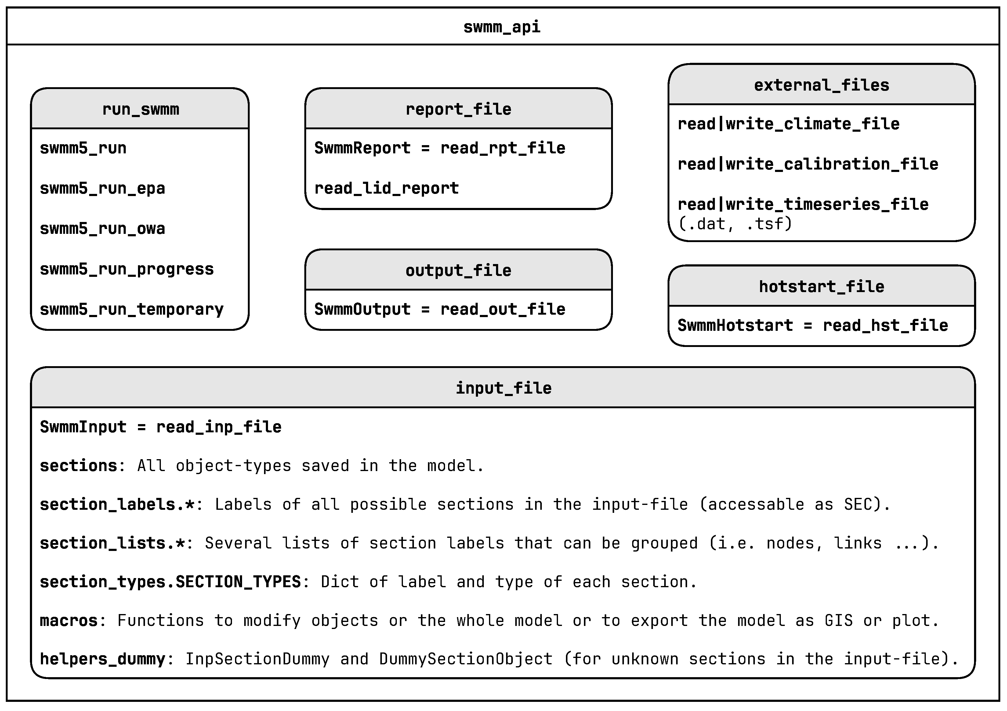Figure 1 shows the modules with their main functions and classes of the package.

2.1. Handling SWMM Input Files

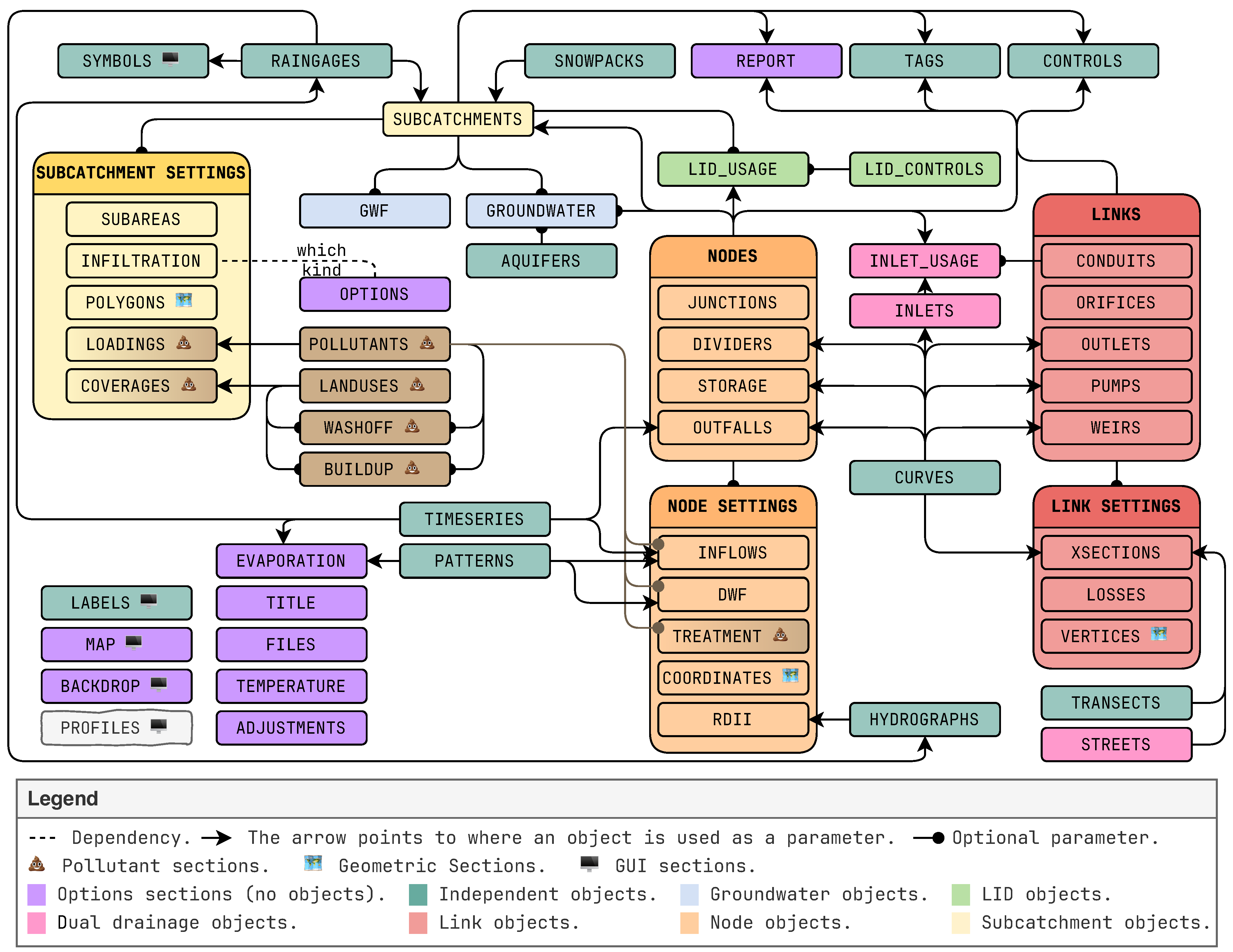
The SWMM input file (*.inp), also known as the project file, is a text-based file that defines the model structure and simulation settings. A key feature of swmm_api is its ability to read and write input files, allowing users to manipulate model structures and input data. The package aligns closely with SWMM’s command-line syntax, making it intuitive for those familiar with SWMM’s source code. Figure 2 displays an overview of all sections in the input file and the connections in between them.

2.1.1. Input File Object Structure

With the input file object, users can read existing input files, create new models from scratch, write new input files, and read, modify, and export specific sections of an input file. If model sections are stored in separate files, the package allows for reading and writing partial input files. The input file object behaves like a dictionary, where sections can be accessed using the section label as a key (inp[‘JUNCTIONS’]) or as an attribute (inp.JUNCTIONS).

Each section is represented as an InputSection object, with two distinct types:

Keyword-value sections, such as OPTIONS, REPORT, FILES, EVAPORATION, TEMPERATURE, ADJUSTMENTS, MAP, and BACKDROP, are managed by InpSectionGeneric. Object-based sections, which include all other sections, are managed by InpSection, where objects have an identifier and associated parameters. These sections use BaseSectionObject to represent a single model element, such as a junction with its parameters. Parameters are accessible via dictionary keys (j1[‘elevation’]) or attributes (j1.elevation). Object-based sections can be converted to pandas DataFrames when all objects share the same parameter types. However, sections are structured as dictionaries by default to handle objects with different attributes. This approach ensures greater generalization while still allowing DataFrame conversion for analysis when applicable.

InputSection objects can be created from scratch, initialized from a string in input file format, and exported as a formatted string, enabling flexible model manipulation.

The sections of an input file are initially read as strings and converted into section objects only when needed. This approach enables fast reading and modification, as unneeded sections remain as strings, improving efficiency. For more details, see Section 4.1.

To fully utilize the package’s capabilities, the focus is on programmatically modifying the model structure, including adjusting parameters.

2.1.2. Input File Macros

Several macro scripts have been implemented, providing automated tools for model analysis, manipulation, and visualization. The following represents the current functionality but can be extended. These scripts can be copied and modified for customized use.

The available macros include structural validation by detecting missing or duplicate objects, combining and splitting dry weather flows at different nodes, and analyzing model structures to track changes across modification steps. Users can convert nodes and links to different types, such as turning a conduit into an orifice, and generate cross-section plots from curve definitions.

Model segmentation is supported by cutting the network at specified nodes and generating inflow series at these nodes based on simulation results. The generated inflow serves as a boundary condition for the newly created segmented network, ensuring continuity in the model. Object management functionalities allow combining, editing, copying, removing, and renaming objects. Dedicated functions allow filtering specific network parts, while a separate function simplifies link vertices to reduce file size for input files or GIS exports.

Geospatial operations include transforming coordinate systems, merging connected sections of links, nodes, or subcatchments into geopandas GeoDataFrame, and exporting these tables in GIS-compatible formats such as Shapefile, GeoJSON, and GeoPackage. A predefined function converts all geometric object data into a combined GeoPackage with QGIS-compatible styles, enhancing GIS integration (see Figure 3).

The package also facilitates network graph operations, including analyzing the pipe network, splitting it at specified nodes, and generating maps of node surroundings. It supports pathfinding between nodes and identifying neighboring elements. Additional tools retrieve upstream and downstream network components, calculate conduit slopes, and compare conduits before merging.

Further features include combining input data objects, plotting sewer network maps, longitudinal profiles, and time series, as well as removing unused objects like control rules, curves, hydrographs, patterns, rain gauges, and other elements to streamline the input file. These capabilities are particularly useful for network segmentation and optimization.

The Python code snippet 1 demonstrates how swmm_api allows users to read an input file, modify specific parameters (such as adjusting the elevation of a junction), access section data as a pandas DataFrame, and save the modified file.

Python Code Snippet 1. Example of using swmm_api to read a SWMM input file, modify a junction’s elevation, access section data as a pandas DataFrame, and save the updated file.

2.2. Processing SWMM Report Files

The SWMM report file (*.rpt) generated after each SWMM simulation is a plain text document containing both the status report and all tables presented in the summary results report. Using swmm_api, data from this text file can be extracted into a structured Python object called SwmmReport. This object organizes the status report primarily as dictionaries and the summary results as pandas DataFrame, accessible through intuitive attributes. Additionally, users can extract specific warnings or errors included in the report file. By leveraging pandas functionality, simulation parameters from the input file can be effectively combined with the simulation outcomes in the report file, streamlining analysis and data manipulation tasks.

The Python code snippet 2 demonstrates how swmm_api can be used to read a report file, extract the node flooding summary as a pandas DataFrame, and merge it with input file data for further analysis.

Python Code Snippet 2. Example of using swmm_api to read a SWMM report file, extract the node flooding summary, and merge it with input file data for analysis.

2.3. Extracting SWMM Output Data

The SWMM output file (*.out) stores all time-series simulation results in a specialized binary format. Using swmm_api, data from this binary file can be extracted into a structured Python object called SwmmOutput. This object contains essential simulation information such as flow units, simulation start date, pollutants modeled, object labels, and parameters.

Results can be conveniently accessed as a single pandas DataFrame, suitable for most small to moderate-sized applications. However, for larger models with numerous objects, loading all results simultaneously can exceed the computer’s available memory. Reading extremely large output files (several gigabytes) can also be slow, and may even fail due to memory limitations, since data typically occupy more memory than the file’s original size. To manage these constraints, the package includes a special memory-efficient reading mode activated by setting the argument slim=True. In this mode, only the necessary time-series data are read incrementally, reducing memory consumption at the expense of increased reading time. Consequently, this option is recommended only when standard data loading exceeds hardware capabilities. For more details, see Section 4.2.

The Python code snippet 3 illustrates how swmm_api can be used to read a output file, extract all time-series results as a pandas DataFrame, and retrieve specific time-series data for a selected node, either by loading the full file or using a memory-efficient mode.

Additionally, pandas functionality allows the data to be exported into compact and performant file formats, such as Parquet, facilitating faster data storage and retrieval.

Python Code Snippet 3. Example of using swmm_api to read a SWMM output file, extract all time-series results, and retrieve specific time-series data with different loading options.

2.4. Support for Additional SWMM File Formats

swmm_api supports additional SWMM-related files beyond the standard input and output files. It provides functionality to read binary hotstart files (*.hst), which store initial simulation states and help accelerate simulation runtimes. Examining these files can offer valuable insights into the model’s internal state at initialization. Additionally, the package allows reading and writing of time-series files (*.dat or *.tsf) that define direct inflows, rainfall, or evaporation data. It also handles climate files containing daily air temperature, evaporation rates, and wind speed, facilitating their seamless integration into SWMM simulations. Furthermore, users can read and write calibration files, which EPA-SWMM uses to generate comparative time-series plots in its graphical user interface, supporting more effective model calibration and validation processes.

2.5. Running Simulations

swmm_api allows users to initiate SWMM simulations directly within the Python environment, enabling automation and batch execution of multiple simulations. Users can specify the executable used for running the simulation, typically the default EPA-SWMM runswmm[.exe] tool. Alternatively, a custom-compiled SWMM binary can be provided, offering flexibility particularly valuable in research contexts. Additionally, the package supports simulations via the Open Water Analytics swmm-toolkit, which conveniently includes pre-compiled binaries for multiple operating systems, such as Linux and macOS, eliminating the need for manual compilation. Another supported approach is using pyswmm [2], a package built upon the swmm-toolkit. pyswmm not only shares the benefits of the toolkit but also allows real-time interaction with ongoing simulations and provides a progress bar, giving users clearer insights into simulation runtime and progress. Additionally, swmm_api enables running SWMM simulations without creating permanent files. Instead, simulations can be executed in a temporary directory, which is automatically deleted after execution. During this process, result files are loaded as Python objects before being removed, ensuring a clean and efficient workflow. This functionality is available through the swmm_api.run_swmm.swmm5_run_temporary function, allowing users to perform simulations without managing intermediate files manually.

2.6. Software Dependencies and Integrations

swmm_api depends on several external Python libraries to extend functionality and facilitate common tasks. The pandas library [12] is central, providing efficient data structures such as DataFrames and Series for handling and analysis of input sections, summary reports, and time-series results. Pandas seamlessly integrates with NumPy, allowing conversion of tables to NumPy arrays, and supports various data export formats like CSV, Excel, and Parquet. Additionally, pandas enables direct plotting with visualization libraries like matplotlib.

The package uses tqdm [13] to display progress bars when reading large input or output files, enhancing user experience in both command-line interfaces and Jupyter notebooks. When simulations are run using pyswmm [2], tqdm also provides visual feedback about simulation progress.

Networkx [14] supports advanced analysis of the pipe network as a graph structure, enabling tasks such as splitting the network at specified nodes, plotting network maps around specific nodes, tracing paths between nodes for longitudinal profile visualizations, and determining upstream or downstream connectivity.

Pyarrow allows efficient export of simulation time-series results to the compact and fast Parquet file format, enhancing data handling and storage performance.

Matplotlib [15] is employed to generate visualizations of sewer network maps, longitudinal profiles, and time-series plots, significantly aiding result interpretation and communication.

For geospatial-related tasks, the package leverages shapely [16], pyproj [17], and GeoPandas [18]. Shapely converts model elements into geometric objects such as points for nodes, line strings for links, and polygons for subcatchments. pyproj handles coordinate transformations and projections, ensuring spatial data are accurately geo-referenced. GeoPandas simplifies the import and export of geometric data, facilitating smooth integration with external GIS software and formats like GeoPackage.

The specialized library SWMM_xsections_shape_generator provides tools to analyze and visualize pipe cross-section geometry. It calculates areas, as well as normal full-flow rates and velocities based on roughness and slope, enhancing the modeling of flow characteristics.

Lastly, pyswmm [2] serves as an optional backend for running SWMM simulations directly within Python. Its advantages include multi-platform support, simulation interactivity, and integration with tqdm [13] to present real-time progress information during simulation execution.

Recommended Software Versions

At the time of writing, the current version of swmm_api is 0.4.66. The package is compatible with Python 3.10 and higher. Its only core requirement is pandas (and its dependencies such as NumPy), with version 2.2 or newer tested extensively, though no compatibility issues have been observed with earlier versions. For extended functionality, the package integrates smoothly with several optional dependencies, including pyswmm (≥2.0), tqdm (≥4.65), matplotlib (≥3.9), geopandas (≥1.0), and networkx (≥3.0). GIS capabilities rely on geopandas and its dependencies shapely and pyproj. To ensure stability across different environments and avoid breaking changes, the development of swmm_api intentionally avoids reliance on deprecated or cutting-edge features in these libraries. This approach enhances long-term robustness and compatibility.

2.7. Source Code and Documentation

The source code of swmm_api is openly available through GitLab (https://gitlab.com/markuspichler/swmm_api, accessed on 26 April 2025) and is distributed via PyPI, enabling straightforward installation using pip install swmm-api. This open-source approach allows users who encounter issues to fix them independently and submit pull requests, facilitating rapid distribution of updates and fixes. Furthermore, open access to the source code enhances transparency and provides users with deeper insights into the underlying implementation.

Users can also contribute by reporting bugs or issues through GitLab’s integrated tracking system. This makes it convenient to document, follow, and address known problems, benefiting the broader user community. Commit histories in the repository clearly indicate when and what changes were implemented, and an automated script parses commit messages to generate an informative changelog accompanying each new release.

Documentation (https://markuspichler.gitlab.io/swmm_api, accessed on 26 April 2025) for the package is primarily generated automatically from source code, ensuring consistency, ease of maintenance, and reduction of redundancy. The documentation website includes a range of example Jupyter notebooks and Python scripts, demonstrating usage from basic tasks to advanced applications. Some of the advanced examples are discussed in the results section; see Section 3.1, Section 3.2 and Section 3.3.

Overall, these practices enhance usability, maintainability, and transparency, supporting active collaboration within the user community.

2.8. Current Limitations and Future Improvements

swmm_api shares no overlapping functionality with the existing package pyswmm [2]. Unlike pyswmm, which interacts directly with simulations using the SWMM C-based API, swmm_api focuses solely on reading, editing, and generating SWMM input and result files independently.

Currently, the package does not perform validation of user-provided parameter values for SWMM inputs. Users must manually ensure data correctness. Any incorrect input data will be identified at runtime by the SWMM simulation binary, with errors subsequently detailed in the simulation report file.

Most functions operate independently of the unit system. However, some macros— particularly those involving GIS integration, such as importing or exporting geospatial data, or updating conduit lengths and subcatchment areas from geometry—are designed exclusively for the metric system. If these functions are called while the input file is configured with imperial units, an error will be raised. Nevertheless, since all macros are implemented as plain Python functions, users can copy and adapt them to support custom unit systems or modify their behavior as needed.

Another limitation arises from differences in case sensitivity: Python string handling is case-sensitive, whereas SWMM’s computational engine is case-insensitive. This discrepancy can lead to unintended duplication of model objects if users do not carefully manage string labels.

While some of these limitations could be addressed in future versions, doing so may require replicating portions of the SWMM C code or compromising the package’s current flexibility. In particular, implementing stricter data validation or unit-specific functionalities would require careful consideration to balance usability and adaptability. The development of such features will largely depend on user demand and specific application needs.

3. Example Applications

To illustrate the capabilities and practical utility of swmm_api, several common use cases involving repetitive tasks or numerous simulations are demonstrated. swmm_api automates SWMM model execution and analysis, enhancing workflow efficiency, repeatability, and reproducibility. By enabling users to create standardized workflows and share them, it directly supports open science initiatives.

• Educational and Operational Applications in Graz

The package already has diverse applications in research and education at the Institute of Urban Water Management and Landscape Water Engineering. It facilitates generating and validating student assignments by automating routine model analysis tasks. In practical applications, it has been successfully utilized to automate regular updates of the SWMM model for the city of Graz by integrating GIS databases of its sewer system. Automating GIS integration has dramatically reduced model update times from weeks to hours, significantly improving efficiency for municipal engineers. The update process involved an existing SWMM model, a polygon layer representing special structures not captured in the GIS database—such as storage tanks and CSOs—that should be retained from the previous model, as well as external inflow points from industrial dischargers and neighboring municipalities with estimated flow rates. The GIS database included updated node-based population data, a digital elevation model (DEM), land cover and soil type layers, a building footprint layer, and a digital sewer asset register containing conduit and junction data.

The workflow delineated subcatchments (SCs) based on the DEM and assigned them to corresponding sewer nodes. SC parameterization was based on literature values derived from land cover and soil type. The sewer infrastructure located within the predefined special structure polygons was copied from the previous model state. Junctions and conduits were then added using the sewer asset register data. Missing parameters were logged for operator review and temporarily filled with best-guess values to ensure the model was executable. A preliminary validation step followed, which again logged incomplete or questionable entries for documentation purposes.

The final model includes approximately 23,000 nodes and links, representing a connected area of 65 km² within the combined sewer system and serving a population of about 300,000. Further details about the model are provided in Pichler et al. [19], where it was used as the base high-resolution model.

The entire workflow was implemented in Python. All data-to-model conversions and object generation were handled using swmm_api.

• GIS Support

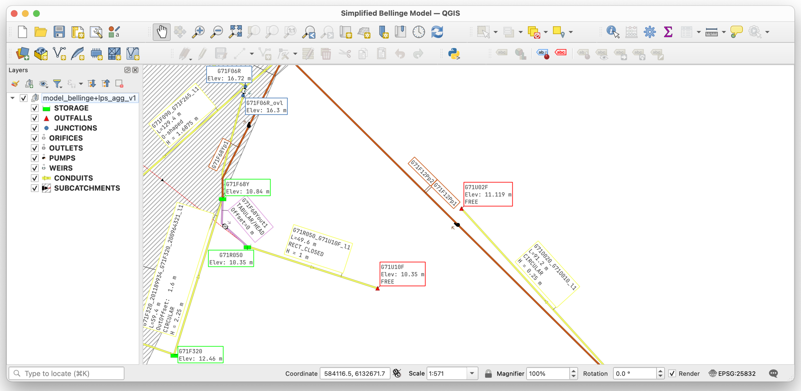
Exploring a SWMM model in GIS software can be essential for analysis and visualization. To support this, swmm_api provides a method to convert model geometries and metadata into GeoPandas GeoDataFrames, which can be exported in GIS-compatible formats such as GeoPackage, Shapefile, and GeoJSON. The GeoPackage export includes predefined QGIS styles, allowing immediate visualization of different object types without manual adjustments. A screenshot of the Bellinge model [11] imported into QGIS using this functionality is shown in Figure 3. The conversion can be performed using the function swmm_api.input_file.macros.write_geo_package.

• Plotting Support

Repetitive tasks such as plotting sewer network maps, longitudinal profiles, and time series can be effectively automated, ensuring consistency across simulations. For instance, the same plotting procedures can be systematically applied to multiple events, such as different design rainfall scenarios or model comparisons, streamlining analysis and visualization. swmm_api provides built-in support for generating these plots.

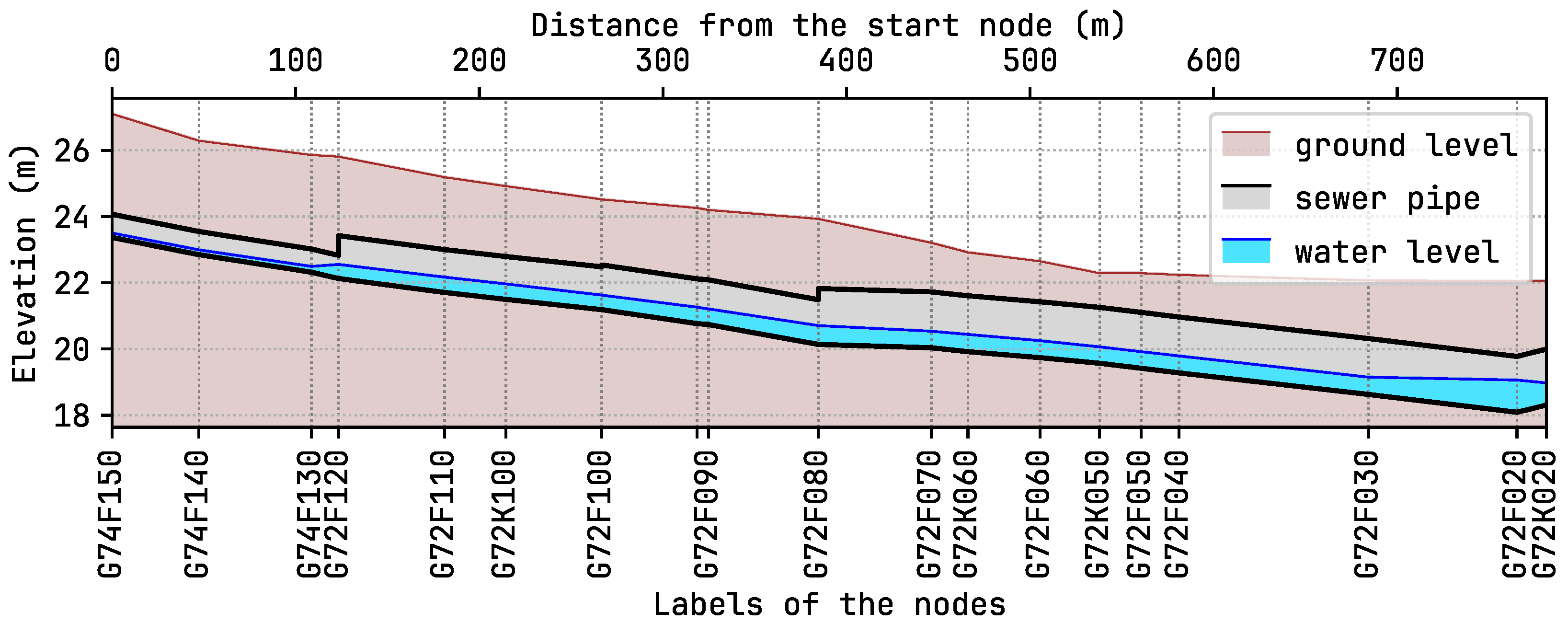
A key example is the generation of longitudinal sewer profiles, which are essential for assessing hydraulic behavior. The function swmm_api.input_file.macros.plot_longitudinal creates these plots, displaying sewer elevation, ground level, and water levels during an event. An example longitudinal profile of the Bellinge model is shown in Figure 4. Additionally, Section 3.3 contains two examples for sewer network map plot of an EPA-SWMM tutorial model.

These use cases emphasize how automation can streamline workflows and enhance reproducibility. The following examples are provided as ready-to-use scripts in the repository, designed to be easily adapted by users to their specific requirements.

3.1. Sensitivity Analysis

One key application demonstrated is sensitivity analysis, essential for identifying the impact of various model parameters on simulation outcomes. Several sensitivity analyses illustrate common scenarios. These analyses are implemented using the SALib package [20] (swmm_api in combination with SALib), with sampling methods based on widely used Sobol sequences.

The first example investigates the sensitivity of subcatchment (SC) parameters, specifically slope, surface flow width, and SC imperviousness. In this case, parameters are uniformly applied to all SCs, examining their influence on total system outlet volume and peak outlet flow rate. Although the example comprises 256 sequential model runs, parallel execution is possible, enhancing performance for larger models or computationally intensive analyses. Extensions could include examining how varying rainfall intensities or durations influence parameter sensitivity, particularly for pervious areas.

Another example explores sensitivity with heterogeneous parameters, varying both the impervious area width individually for each SC and the conduit roughness grouped by predefined tags. This scenario assigns identical parameter values to conduits sharing the same tag. The resulting sampling includes 384 parameter sets, highlighting the package’s flexibility in handling complex, tagged parameter variations and demonstrating targeted analyses of individual or grouped model elements.

The code for these example cases is available in the package repository (https://gitlab.com/markuspichler/swmm_api/-/tree/main/examples/advanced_examples/sensitivity_analysis, accessed on 26 April 2025).

3.2. Model Calibration and Uncertainty Assessment

The calibration and uncertainty analysis capabilities of swmm_api are demonstrated through a practical workflow employing the SPOTPY optimization framework [21]. Initially, an SWMM base model is calibrated by varying SC parameters such as surface width and imperviousness. Calibration involves defining these parameters as uniform probability distributions within SPOTPY. During calibration, the package systematically adjusts these SC parameters and executes simulations, producing modeled catchment outlet flow rates. These results are compared against synthetic observational datasets, generated by perturbing model results to simulate measurement uncertainty.

The calibration employs SPOTPY’s optimization algorithms to iteratively explore parameter combinations, using the Nash–Sutcliffe Efficiency (NSE) as the objective function. Specifically, the SC parameter width and imperviousness are optimized using uniform distributions to identify parameter sets that best reproduce the (synthetic) observed flow data. After completing calibration runs, the model is updated using the optimal parameter values, resulting in a calibrated SWMM model with improved predictive accuracy and reliability.

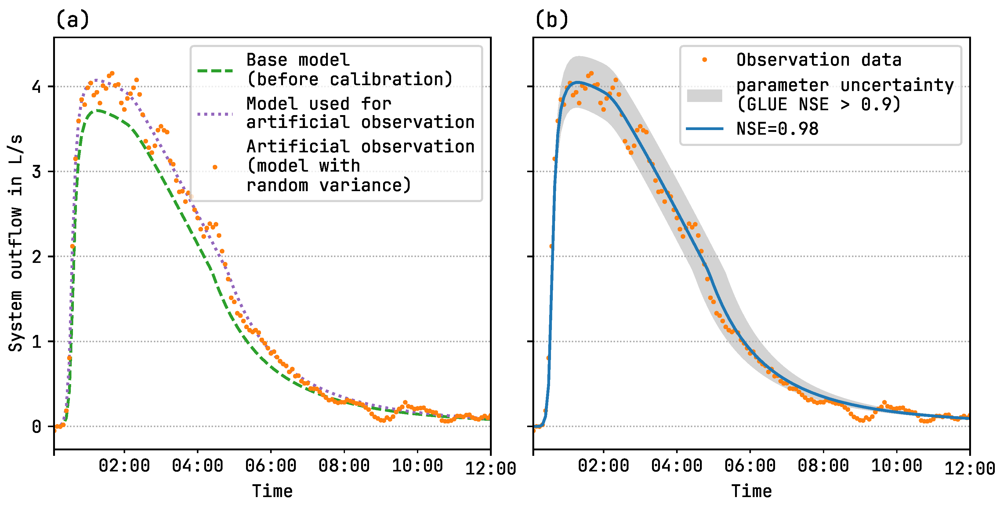
Additionally, uncertainty analysis is demonstrated using the Generalized Likelihood Uncertainty Estimation (GLUE) method. In this context, GLUE identifies parameter sets yielding acceptable simulation performance, defined by exceeding a chosen threshold of the NSE. This approach helps quantify parameter uncertainty, thereby informing users about model reliability and supporting informed decision-making in urban drainage management.

The effectiveness of the calibration and uncertainty analysis workflow is illustrated in Figure 5. Figure 5a shows the time series of the base model before calibration, the model used to generate artificial observations, and the synthetic observations with added random variations. Figure 5b presents the observed data alongside the calibrated model, achieving an NSE of 0.98, and the uncertainty range estimated using the GLUE method with an NSE threshold of 0.9.

The code for this example application, including plot generation, is available on the documentation website (https://markuspichler.gitlab.io/swmm_api/examples/calibration_and_uncertainty, accessed on 26 April 2025).

3.3. Reproducing EPA-SWMM Tutorials in Python

The official EPA-SWMM documentation provides a series of tutorials demonstrating key modeling tasks performed through its graphical user interface (GUI). To illustrate the applicability and convenience of scripting, the same tutorials have been replicated with swmm_api. Both the package repository (https://gitlab.com/markuspichler/swmm_api/-/tree/main/examples/epa_swmm_samples_5_2, accessed on 26 April 2025) and the documentation website (https://markuspichler.gitlab.io/swmm_api/examples/index.html#epa-swmm-examples, accessed on 26 April 2025) include these tutorials, showcasing how identical modeling tasks can be effectively completed using Python scripts instead of the GUI.

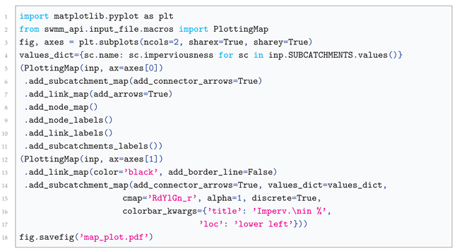
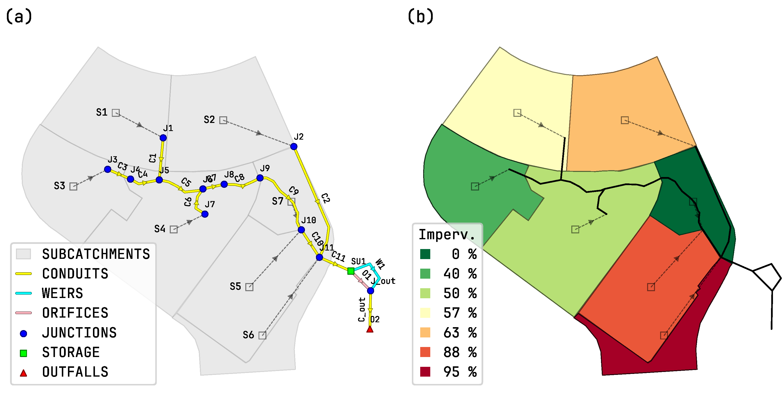
As an example, Figure 6a presents a map plot of the EPA-SWMM tutorial “detention pond model” generated using swmm_api, highlighting key model elements. In Figure 6b, subcatchments are colored based on imperviousness, but they can also be visualized based on simulation results extracted from the report or output file, enabling further analysis and interpretation. The corresponding implementation is provided in code snippet 4.

Python Code Snippet 4. Generating map plots of the EPA-SWMM tutorial “detention pond model”. The resulting plots are shown in Figure 6.

3.4. Usages in Scientific Literature

Farina et al. conducted over 40,000 simulation runs, generating individual input files and analyzing output data—an approach made feasible by swmm_api’s batch processing and parallel computing capabilities [22]. In a later study, Farina et al. utilized swmm_api for sensitivity analysis, executing 10,000 simulations with varying parameter sets [23].

Baumann et al. and van der Werf et al. extracted simulation results within a Python workflow using swmm_api [24,25], while van der Werf et al. leveraged it for interfacing with input files [26].

Zhang et al. applied swmm_api to manipulate project files when testing real-time control strategies with reinforcement learning [27], and Zhang et al. used it to train a machine learning surrogate model [28].

Pichler et al. employed swmm_api to derive a simplified model from a high-resolution counterpart by analyzing and modifying network structures, optimizing accuracy, and publishing their code on GitHub [19]. Farina et al. used swmm_api in a similar research context [29].

Ryrfors Wien used swmm_api for batch simulations, output analysis, and model calibration, and made the developed code publicly available [30]. Similarly, Pritsis et al. utilized swmm_api to simulate and analyze ensembles of hyetographs [31].

4. Benchmarks

The following benchmarks were conducted on a MacBook Pro (2021) with an Apple M1 Pro chip (Apple Inc., Cupertino, CA, USA), 16 GB of memory, running macOS 15.4 and Python 3.12. The tests evaluate memory usage and execution time for reading SWMM input and output files of varying sizes and object counts.

4.1. Reading and Editing SWMM Input Files

A direct performance comparison with pyswmm is not feasible, as pyswmm does not allow modifying input parameters. It only provides access to initial and current state values during simulation, without support for structural input file manipulation.

This benchmark evaluates three key operations:

• Reading the input file as a plain string.
• Reading the file and converting all sections to Python objects.
• Reading the file and modifying a single parameter of one object.

Table 1. Benchmark results for reading and editing five different SWMM input files. “String” refers to loading the file as plain text. “Objects” indicates loading the file and converting all elements into Python objects. “Edit” involves loading the file and modifying a single parameter of one object.

Filesize	Number of Objects			Execution Time in s			Memory Usage in MiB
MB	Links	Nodes	Subcat.	String	Objects	Edit	String	Objects	Edit
0.17	23	16	7	0.00081	0.032	0.0013	0.33	0.36	0.33
0.98	422	422	805	0.0022	0.094	0.0036	1.9	1.9	1.9
1.2	1044	1020	713	0.0027	0.12	0.0041	2.3	1.6	2.3
110	1788	1612	1451	0.2	15	0.27	210	400	210
16	24,101	23,920	13,405	0.026	1.4	0.036	31	1	31

presents the benchmark results for five input files of varying sizes and complexities. To provide context, the file size and number of links, nodes, and subcatchments are included. Notably, the 110 MB file contains polygon definitions for subcatchment geometries. Despite having fewer network objects, its larger size reflects the added geometric detail.

Interestingly, memory usage is lower when parsing the file into SWMM object types than when reading it as a plain string. This is due to the compact representation of model elements in swmm_api.

When editing a specific section, only that section is converted into Python objects. This selective parsing improves performance and is reflected in the reduced execution time observed in the “edit” benchmark compared to full object parsing.

Each benchmark scenario was repeated ten times, and the reported values represent the averaged results to ensure robustness.

4.2. Reading SWMM Output Files

This benchmark compares six SWMM output files that vary in model complexity, simulation duration, and outcome—including one file where the simulation failed. The goal is to assess performance and scalability when reading different numbers of result columns, ranging from a few selected series to the entire dataset.

The following methods were compared:

• The official EPA-SWMM Python package, which uses the SWMM C API (epaswmm).
• pyswmm, also based on the SWMM C API.
• swmm_api with slim=False, reading the entire output file into a NumPy array.
• swmm_api with slim=True, reading only the required columns on demand.

Table 2. Memory usage in MiB for reading six different SWMM output files. “*” indicates an aborted simulation; “?” marks cases where extrapolation was not feasible; “-” denotes cases with fewer columns available in the file.

				Number of Read Columns
Filesize	Periods	Columns	Package	1	10	100	1000	10,000	100,000	Full
820 KB	720	282	epaswmm	0.34	0.86	6.35	-	-	-	21
			pyswmm	0.34	0.85	6.34	-	-	-	21
			swmm_api	0.84	0.94	1.96	-	-	-	4
			swmm_api(slim)	0.05	0.35	3.38	-	-	-	9.5
215 MB	2881	18,627	epaswmm	1.7	3.7	26	252	?	-	?
			pyswmm	1.3	3.4	25	251	2510	-	?
			swmm_api	210	210	213	253	654	-	1037
			swmm_api(slim)	2.2	2.5	14	133	1325	-	?
3.2 GB	47,280	17,059	epaswmm	22	58	433	?	?	-	?
			pyswmm	22	58	433	?	?	-	?
			swmm_api	3083	3089	3154	3803	10,301	-	15,397
			swmm_api(slim)	3.4	23	219	2182	?	-	?
1.7 GB	1620	264,040	epaswmm	6.2	7.2	20	139	1333	?	?
			pyswmm	15	1.8	16	135	1329	?	?
			swmm_api	1711	1711	1711	1720	1947	4219	8359
			swmm_api(slim)	35	35	35	92	775	?	?
19 MB *	17 *	264,040	epaswmm	not possible
			pyswmm	not possible
			swmm_api	96	96	96	96	97	156	281
			swmm_api(slim)	35	35	35	35	35	146	359
27 GB	525,600	12,746	epaswmm	230	554	?	?	?	-	?
			pyswmm	230	554	?	?	?	-	?
			swmm_api	not possible
			swmm_api(slim)	29	250	2457	?	?	-	?

presents the memory usage results from the benchmark tests. A key finding is that when swmm_api reads the full output file internally, the memory usage initially matches the file size. However, as more columns are loaded, memory demand increases—reaching up to five times the file size when all columns are read. This increase is primarily due to the overhead from pandas during DataFrame conversion. Despite this, swmm_api with slim=True consistently requires less memory than both pyswmm and epaswmm in nearly all scenarios.

Table 3. Execution time in seconds for reading six different SWMM output files. “*” indicates an aborted simulation; “?” denotes cases where extrapolation was not feasible; “-” signifies fewer columns available in the file. Red numbers indicate extrapolated values.

				Number of Read Columns
Filesize	Periods	Columns	Package	1	10	100	1000	10,000	100,000	Full
820 KB	720	282	epaswmm	0.016	0.061	0.63	-	-	-	2.3
			pyswmm	0.019	0.052	0.48	-	-	-	1.6
			swmm_api	0.002	0.003	0.004	-	-	-	0.006
			swmm_api(slim)	0.004	0.019	0.16	-	-	-	0.45
215 MB	2881	18,627	epaswmm	0.05	0.26	3.0	31	300	-	540
			pyswmm	0.06	0.22	2.3	22	220	-	390
			swmm_api	0.18	0.17	0.17	0.2	0.4	-	0.7
			swmm_api(slim)	0.09	0.14	0.71	6.4	65	-	120
3.2 GB	47,280	17,059	epaswmm	1.0	4.9	50	500	5000	-	8500
			pyswmm	3.7	34	350	3500	35,000	-	60,000
			swmm_api	1	1	1	1.5	7	-	11
			swmm_api(slim)	0.6	1.3	11	120	1200	-	2000
1.7 GB	1620	264,040	epaswmm	0.06	0.18	1.6	17	180	1800	4600
			pyswmm	0.04	0.12	1.2	12	120	1200	3200
			swmm_api	2.3	2.3	2.3	2.3	2.5	5	13
			swmm_api_slim	0.9	1.0	1.3	4.5	37	370	980
19 MB *	17 *	264,040	epaswmm	not possible
			pyswmm	not possible
			swmm_api	2.1	2.1	2.1	2.1	2.2	3.5	5.7
			swmm_api(slim)	0.9	0.9	0.9	1.0	1.7	15	45
27 GB	525,600	12,746	epaswmm	38	350	?	?	?	-	?
			pyswmm	38	350	?	?	?	-	?
			swmm_api	not possible
			swmm_api(slim)	38	43	240	?	?	-	?

shows the execution time for reading the output files. For small files or when reading a limited number of columns, all approaches perform similarly. However, as file size and the number of columns increase—or when reading incomplete files—swmm_api demonstrates a significant performance advantage.

In pyswmm, epaswmm, and swmm_api with slim=True, time-series data are read column by column using a loop. This approach incurs a significant performance penalty due to Python’s slower loop execution. In contrast, when swmm_api loads the full file (slim=False), it uses a vectorized NumPy-based method implemented in C, offering far better performance. In this case, the number of columns has only a minor impact on read times—differences are mainly due to the subsequent conversion of the NumPy array to a pandas DataFrame.

Another key distinction is that both epaswmm and pyswmm packages cannot process output files from simulations that failed or were aborted (e.g., due to disk space limitations). In contrast, swmm_api can read such files, enabling analysis of incomplete or failed runs.

5. Conclusions

The swmm_api Python package significantly enhances efficiency and flexibility in urban drainage modeling using SWMM. By enabling direct manipulation of SWMM input and output files within Python, it streamlines tasks such as model creation, calibration, sensitivity analysis, and visualization. Unlike pyswmm, which focuses on real-time simulation interaction through SWMM’s C-based API, swmm_api provides a comprehensive suite of tools for pre- and post-simulation activities, operating independently of the simulation engine.

The package features an intuitive, dictionary-like structure for efficient data handling, allowing users to easily modify and analyze SWMM models. Seamless integration with Python’s extensive ecosystem—including libraries for GIS processing, data analysis, and machine learning—further broadens its applicability in both research and practical applications. Additionally, its automation capabilities significantly reduce the time required for repetitive modeling tasks, improving workflow efficiency and reproducibility.

By filling critical gaps left by existing tools, swmm_api provides a powerful, flexible, and user-friendly solution for SWMM model management. Its contributions to automation, data analysis, and reproducibility make it a valuable asset for researchers and practitioners working in urban water management.