Comparing SWMM and HEC-RAS Hydrological Modeling Performance in Semi-Urbanized Watershed

Abstract

One of the most common applications of hydrological models is in studying urban watersheds, with distributed and semi-distributed models being used more frequently. The choice of modeling tools and the selection of hydrological processes to represent is dependent on the modeling objectives, available resources, and the scale of the study. Certain modeling setup parameters can have important effects on model accuracy, such as the representation of aquifer components, detailed surface storage, and discretization, among others. The effects of these parameters are often unknown since most hydrological studies do not systematically alter these parameters nor consider different modeling tools. This study performs a comparative analysis between SWMM and HEC-RAS in describing the hydrological response of a semi-urbanized headwater watershed in Alabama. Within each model, different modeling parameters were varied and the effects on the model accuracy were assessed with the stream depth and velocity collected in the field. The results showed that the parameters most impactful in SWMM modeling results were the existence of an aquifer component as well as the careful representation of surface storage. Conversely, HEC-RAS results were comparable with SWMM results when an aquifer was not present, but the runoff was highly overpredicted when infiltration was not considered. These results can indicate the applications and limitations of rain-on-grid model results that neglect interactions with shallow groundwater.

1. Introduction

Hydrological models are a useful tool for analyzing the impact of urban development on watersheds. Construction activities and changes in surface permeability can create a significantly higher runoff volume, flow rate, and sediment loading, which, if not properly planned for, can cause flooding downstream [1] and contribute to stream impairment [2]. Models can be used to predict the effects of these activities and determine the best management practices (BMPs) for mitigating any negative consequences [3].

Several types of modeling tools have been created for hydrological modeling, which can be classified according to spatial structures as lumped, semi-distributed, or fully distributed [4]. Lumped models, such as the Rational Method, simplify watersheds by averaging characteristics over the whole area of interest. Fully distributed and semi-distributed models utilize spatial discretization to break up a watershed into smaller units, i.e., sub-watersheds or grid cells, based on similar physical and hydrologic characteristics [5]. Some of the more widely used of these include the EPA Stormwater Management Model (SWMM) [6] and the Hydrologic Engineering Center-River Analysis System (HEC-RAS) [7].

The SWMM is a semi-distributed hydrological model that divides a watershed into several subcatchments. Since its initial development in the 1970s, the SWMM has evolved from a surface hydrological model to include capabilities such as shallow groundwater interactions, water quality changes, and the effects of low-impact development controls (LIDs). Commercial versions of the SWMM have enabled the integration of specialized tools, for instance incorporating geospatial databases [5,8]. It is commonly used in designing man-made stormwater sewer systems to mitigate combined sewer overflow, designing detention ponds to achieve a pre-development outflow, and evaluating the effectiveness of LIDs and BMPs in mitigating stream pollution [3,9]. To a much lesser extent, the SWMM is used for the modeling of natural watersheds, including comparing pre- and post-development hydrological conditions and identifying potential groundwater resources [10,11].

The HEC-RAS (version 6.3.1.) is a software developed by the U.S. Army Corps of Engineers (USACE) initially designed for representing river hydraulics through one-dimensional (1D) formulations. Later, in 2016, the HEC-RAS included two-dimensional (2D) unsteady flow modeling [12] by representing structured and unstructured grid cells in a solution domain. With the 2D modeling capabilities, the HEC-RAS also enabled the representation of overland flows created by rain-on-grid simulations, and subsequently abstractions through CN or Green-Ampt infiltration. Even though at its core the HEC-RAS is a hydrodynamic modeling tool, it has some of the features commonly found in hydrological models. However, unlike other hydrological modeling tools, such as the SWMM or Hydraulic Engineering Center Hydrologic Modeling System (HEC-HMS) [13], the HEC-RAS is not adapted to represent extended period simulations.

Regardless of the hydrological tool, an important modeling consideration is the level of detail in representing surface and sub-surface hydrological processes in a watershed. Both can affect the quality of the results and determine the computing power and time required to run a simulation [7,14]. Discretization refers to both the number of parts, such as the number of subcatchments, channels, and junctions for semi-distributed models, or the grid density for fully distributed models, as well as the number of processes being simulated at once for each part. According to the modeling goals, the representation of hydrological processes, such as infiltration, groundwater exfiltration, or evapotranspiration [14], can increase accuracy at the cost of longer simulations. For larger scale applications, such as in watershed management planning, high levels of detail may not be possible due to limited resources [15]. Models like the SWMM and HEC-RAS are frequently used because of their relative simplicity and comparatively lower data input requirements [16].

Many studies have been conducted on the effects of discretization on the accuracy of models, with no consensus about whether finer discretization is better for model output [9]. The study by [17] in the Faneuil Brook subbasin of Boston (~4.6 km²), a mostly residential watershed [18], observed a dual-scale effect whereby the aggregation of the model—decreased discretization—decreased the peak runoff and outflow for large storms and increased it for smaller storms. This was attributed to the simplified infiltration, longer overland flow lengths, and simpler conduit routing. The study by [19] of a 2.66 ha urban street in the Bronx, New York, observed a different dual-scale effect where a higher discretization model was slightly better for an extended simulation, while the lower discretization model performed better for individual events. The study by [20] found that increasing the subcatchment discretization of a city-block-sized watershed (~0.5 ha) in Wilmington, North Carolina had an almost negligible effect on the volume and peak flow. In two-dimensional hydrodynamic modeling, spatial discretization substantially influences the computational accuracy and simulation efficiency [21]. A study in a small rural catchment (2.13 km²) of the Gersprenz River in Germany [22] found that using coarser cell sizes greater than 10 m delayed and attenuated the outflow hydrograph and reduced the runoff volume. Similarly, ref. [23] observed comparable effects when increasing the mesh resolution from 50 m to 100 m, analyzing a large rural mountain watershed (10.5 km²) in Norway. In contrast, the study by [24,25] within a 56 km segment of the River Yesil (Ishim) in Kazakhstan and a 13.75 km² catchment in the Lombardy Region of Italy, respectively, found that variations in mesh size had no discernible impact on the flood hydrograph. However, both studies noted considerable reductions in the simulation time with coarser meshes. These findings highlight the complexity of mesh resolution decisions at different basin scales in 2D HEC-RAS modeling.

The work by [15], in anticipation of regional scale applications of the SWMM, investigated the prediction of suspended solid concentrations with a coarse model of a large, developed watershed (10 mi²) in Dallas, Texas. A limited calibration of only two parameters yielded generally acceptable results. More recent studies into regional scale applications, such as the 52.6 km² Attanagalu Oya basin in Sri Lanka [26], have shown that parameters like channel roughness become less significant as the stream order increases, while intermittent storage is more significant to recession curve modeling. Similarly, recent studies indicate that the HEC-RAS’s rain-on-grid modeling can reliably reproduce observed hydrographs with a minimal parameter calibration. For instance, ref. [27], in the 45 km² Rainbow Creek basin in Ontario, and [23], in a 10.5 km² basin, achieved a good agreement with observed peak flows during short-duration storm events by calibrating the Curve Numbers and channel roughness coefficients, although minor discrepancies were noted in the recession limbs. Furthermore, a study in rural parts of northwest Italy by [28] comparing HEC-RAS hydrographs to synthetic design hydrographs from traditional hydrologic methods found that while the peak discharges were well matched for rare, large storms, the total runoff volumes were lower in HEC-RAS simulations. In multi-peak events, ref. [23] noted that the model struggles to accurately reproduce secondary peaks due to the absence of subsurface return flows, leading to a runoff underestimation during successive peaks.

Many studies have previously been conducted into the SWMM and HEC-RAS focusing on urban watersheds. Some focused on the integration between the two models where the SWMM hydrological results were fed into the HEC-RAS for flow calculations or to predict flood inundation [29,30,31]. Others compare results between the two models to benchmark the calibration or determine the suitability of use in certain conditions [32,33,34]. For example, ref. [32] found that the SWMM and HEC-RAS may both be suitable for modeling the flow in urban catchments around the Służewiecki Stream in Warsaw, Poland. However, comparisons of the two tools for hydrological modeling are not as common. Presently, there is much interest in the HEC-RAS as a hydrological modeling tool due to its rain-on-grid capabilities and relatively low data requirements. However, this model has not been conceived as a hydrological model, and thus it has limitations, such as groundwater modeling, which have not been fully explored.

This study seeks to contribute to this field of research by comparing the effects of various modeling parameters for the SWMM and HEC-RAS 2D in representing the hydrology of a semi-urban watershed. The question this study addresses is what hydrological modeling parameters are most significant to the representation of the runoff and stream flow for the purposes of hydrological watershed management planning. This parameter evaluation is performed individually and in combination on the projected volume of runoff and total flow and the accuracy of the depth and velocity results compared to measured data using simplified hydrological models for extended period simulations.

2. Materials and Methods

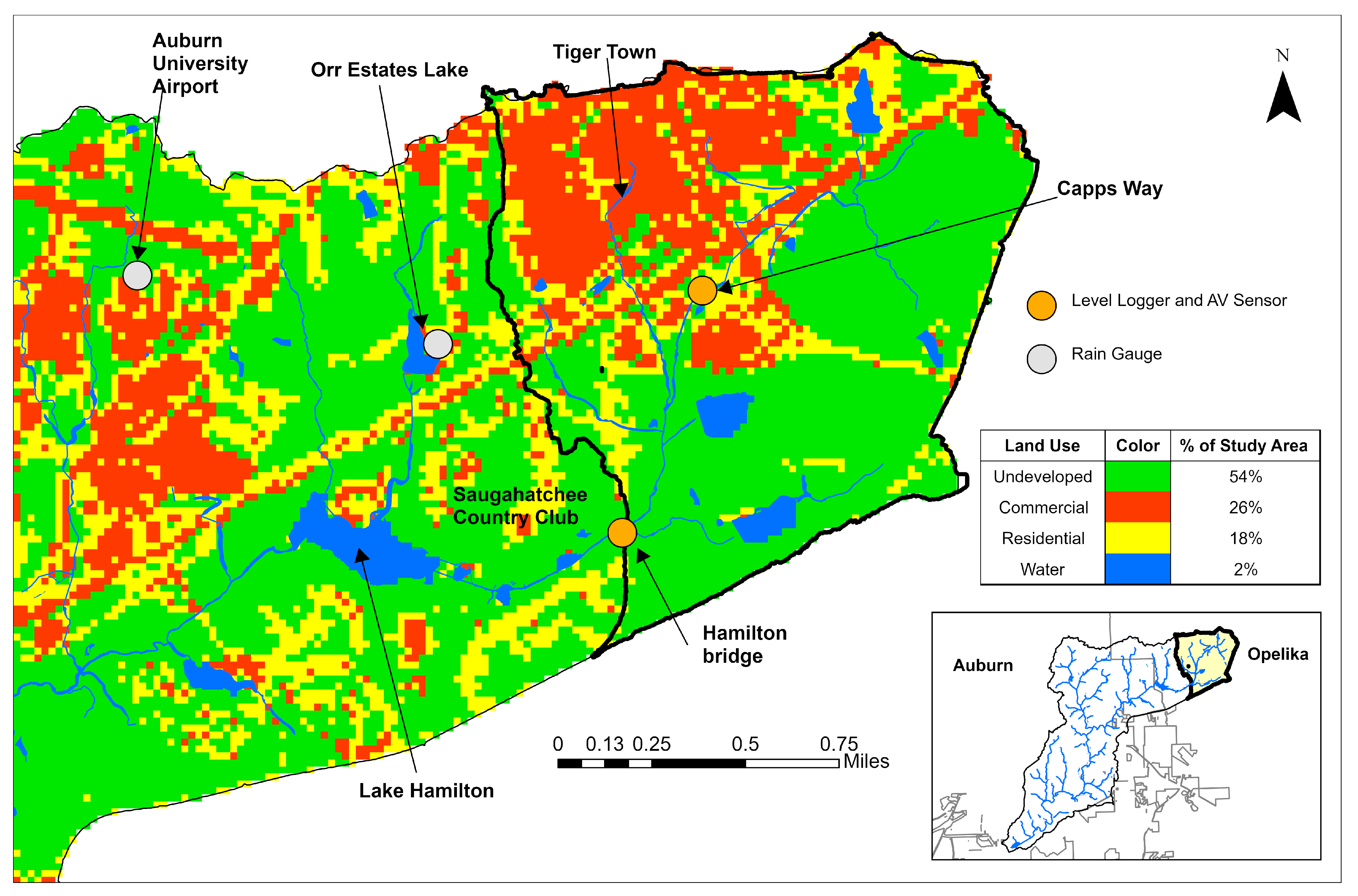
2.1. Field Work

This study was conducted in the Moore’s Mill Creek (MMC) watershed, located in Lee County, Alabama as part of a larger project linked to the watershed management plan update. The watershed has become impaired by siltation in recent years, likely due to the rapid development of the cities of Auburn and Opelika and related construction site runoff impacts. This study focuses on part of the Opelika portion of the watershed, shown in Figure 1, covering an area of approximately 400 ha (4 km²). This part of the watershed covers a mix of low- to high-intensity development, simplified as residential and commercial land uses, and undeveloped forested areas and open spaces. Notable land uses include the Tiger Town shopping center, Saugahatchee Country Club, and I-85. Figure 1 below shows the location of stream monitoring stations and a breakdown of the land usage.

The data used for the calibration of the hydrological models were collected as part of a previous study [35] in the same watershed, including rainfall and stream depth measurements from December 2021 to January 2022. Newer measurements of the stream depth and velocity were collected between November 2024 and January 2025 to develop head-velocity curves of the same sites. These curves were used to hindcast velocity hydrographs for the calibration dataset as there have been no significant morphological changes to the watershed since the previous study.

Table 1. Location and type of data collected at monitoring station.

Location	Data Collected
Capps Way	Stream depth, stream velocity
Hamilton bridge	Stream depth, stream velocity
Auburn University Airport	Rainfall
Orr Estates Lake	Rainfall

lists the locations and type of data collected at each station.

The stream depth was measured using Onset (Bourne, MA, USA) HOBO U20L-04 level loggers rated for depths up to 4 m (13 ft) and with an individual accuracy of ±0.3% [36]. One logger was used to measure the atmospheric pressure to correct depth measurements, with an estimated combined error of ±2 cm (1 in). Readings were synchronized for all devices to occur at fifteen-minute intervals.

One Onset HOBO RG3 rain gauge with a 0.2 mm (0.01) resolution and accuracy of ±1.0% was deployed at a centralized location within the watershed to measure rainfall [37]. These were stationed at the Auburn University Airport for the previous study [25] and at Orr Estates Lake for more recent data. The data were processed to count the number of bucket tips in five-minute intervals and input as the model rain gauge.

One Teledyne Isco (Lincoln, NE, USA) 2150 area-velocity (AV) sensor was deployed at two separate locations within the watershed to measure stream depth and velocity. The AV sensor is rated for velocities ranging from −1.5 to 6.1 m/s (−5 to 20 ft/s) in streams at least 25 mm (0.8 in) deep with an error rating up to ±2% [38]. The sensor collected data at the selected stations for several weeks before being relocated due to limited equipment availability. Readings were taken at 30 min intervals when water depth was below 5 inches and at 5 min intervals when it was above the threshold. A head-velocity curve was created for both stations to predict the velocities from historical readings assuming stream conditions were similar enough between studies.

2.2. SWMM Implementation

This study specifically uses Personal Computer Storm Water Management Model (PCSWMM), a commercial version of SWMM5 developed by Computational Hydraulics Incorporated (CHI). PCSWMM comes with several additional tools used in the setup and calibration of models for this study. Several tools enable the use of digital elevation maps (DEMs) to automatically delineate a watershed based on an outlet, including the following: the number, slope, and area of subcatchments; the length, direction, and geometry of channel conduits; and the elevation and location of junctions. The Sensitivity-Based Radio Tuning Calibration (SRTC) allows fine tuning of specific model parameters with immediate feedback about the effects on the resulting hydrographs.

The watershed was set up using several DEM integrated tools. The watershed delineation tool (WDT) utilized a 1 m × 1 m Light Detection and Ranging (LiDAR) map [39] to create and place subcatchments, junctions, and conduits. Additional tweaking was made to correct the stream network according to [40,41]. Junctions were moved or created to accommodate these changes and set with a new elevation based on the DEM. Channel cross-sections were created with the “Transect Creator” tool where the stream was above ground. The culverts crossing the southern part of the I-85 interchange were assumed to be 1.2 m tall by 4.2 m wide based on field measurements. Culverts crossing I-85 and underground drainage pipes in Tiger Town were left as 1 m diameter pipes due to a lack of data. Dimensions for hydraulic structures for reservoirs were sourced from Table 3.3 of [35].

Several parameters were generalized for this study based on the recommended values from the literature, including Manning’s roughness values [8] and depression storage [6], as they were not deemed crucial given the goals of this research. Several systematic corrections were applied accounting for baseline flows [35] and inlet offsets at monitoring locations, a correction suggested in [42]. These parameters are listed in

Table 2. General parameters for SWMM.

Surface	Manning’s Roughness (n)		Depression Storage (Dstor)
	n	Range	Dstor	Range
Overland pervious	0.30	0.20–0.40	4 mm	2.5–8.0 mm
Overland impervious	0.011	0.010–0.019	2 mm	1.0–2.5 mm
Natural channel	0.30	0.20–0.40	-	-
Culvert and sewer	0.011	0.010–0.019	-	-

.

Curve Number (CN) infiltration was utilized in this study with the cutoff method researched by [35]. A fully composite approach, as used in SWMM or WinTR-55, assumes all surfaces are pervious regardless of their CN and uses the average value for the input parameter. The cutoff approach assumes that values above a certain threshold—a CN of 90 for this study—are practically impervious. The average is taken from the pervious surfaces, and an impervious percent is calculated from the remainder. The “Curve Number Generator” plugin [43] for QGIS was used to generate a CN map on a 30 m by 30 m grid scale based on the National Land Cover Dataset (NLCD) [44] and Soil Survey Geographic Database (SSURGO) [45] reference tables. The cells were assigned based on the subcatchment they fell within according to a shape file of the SWMM subcatchments. A Visual Basic code was developed for Microsoft Excel that calculated the average CN of pervious surfaces, those below the cutoff value of 90, and the percentage of impervious surfaces for each subcatchments.

A limited sensitivity analysis was conducted to analyze the effects of four modeling parameters on the depth, velocity, flow rate, total flow volume, runoff volume, and, for SWMM alone, total exfiltration volume in this watershed:

• The first of these modeling parameters was overland flow path length. When using WDT, PCSWMM automatically calculates flow width using the method by [46] and flow length by dividing the area by the flow width. This value is dependent on the subcatchment size and can vary broadly. It was decided to compare scenarios with the automatically calculated flow length to those with a manually designated maximum length of 150 m (500 ft) [47] to see if this adjustment was necessary for accurate results.
• The second modeling parameter was the representation of storage basins within the subcatchments. SWMM applications for urban watersheds consider storage basins in terms of artificial detention and retention ponds where geometry is known. This sub-watershed, in addition to detention ponds for Tiger Town, features several surface ponds of unknown depth and varying dimensions as part of the MMC stream network. This study compared models where these basins were and were not included as storage objects in the model. These basins utilized a simplified geometry, assuming a constant area with depth due to a lack of bathymetric data.
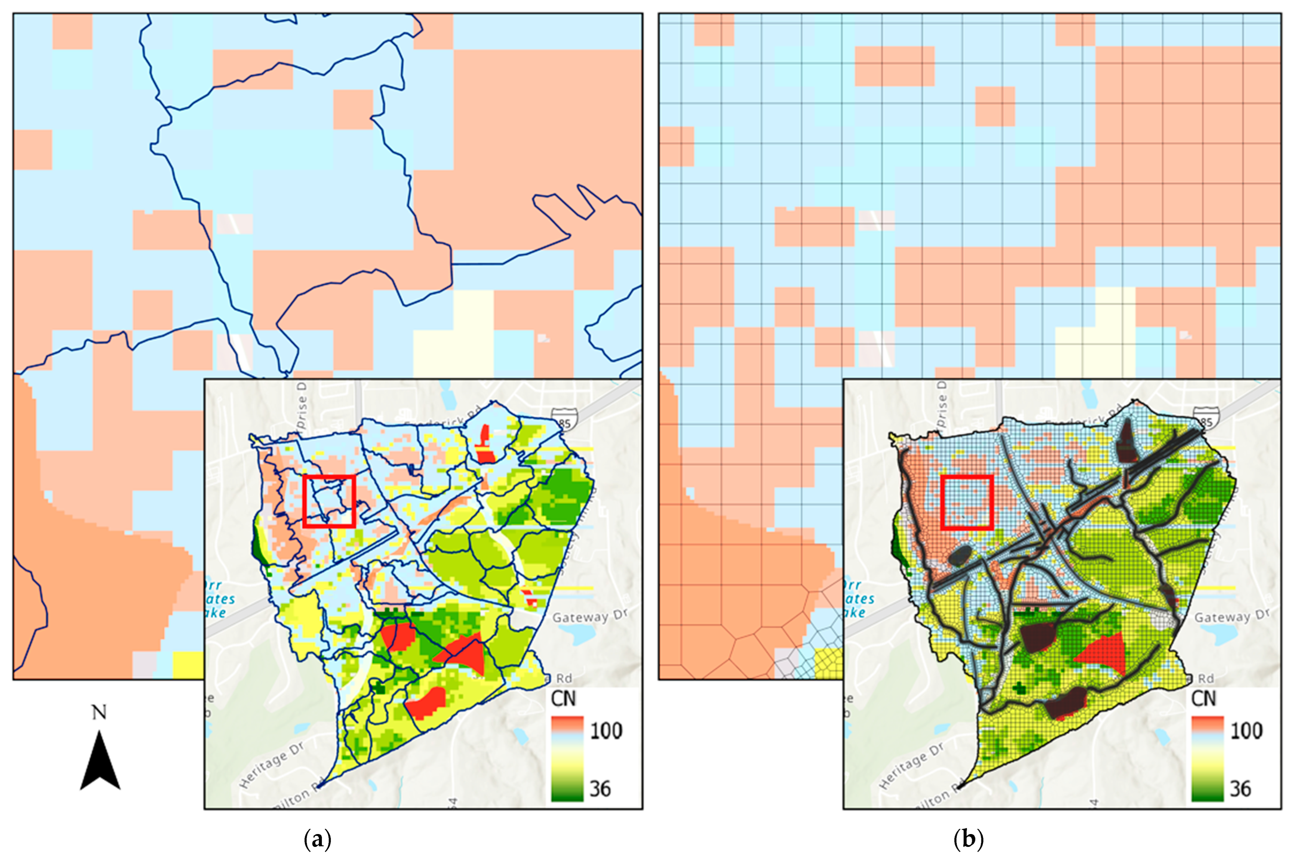
• The third modeling parameter was linked to the target discretization size of subcatchments in the SWMM simulation. Models such as HEC-RAS utilize a two-dimensional rain-on-grid approach for calculating runoff and overland flows. Initial comparisons of SWMM and HEC-RAS results for this watershed showed that HEC-RAS models had better representation of hydrograph drawdown. This was initially theorized to be due to the higher level of discretization possible with HEC-RAS. Two sizes of subcatchment discretization area were tested for this study to see the effects of increasing subcatchment density: 10 ha and 5 ha.
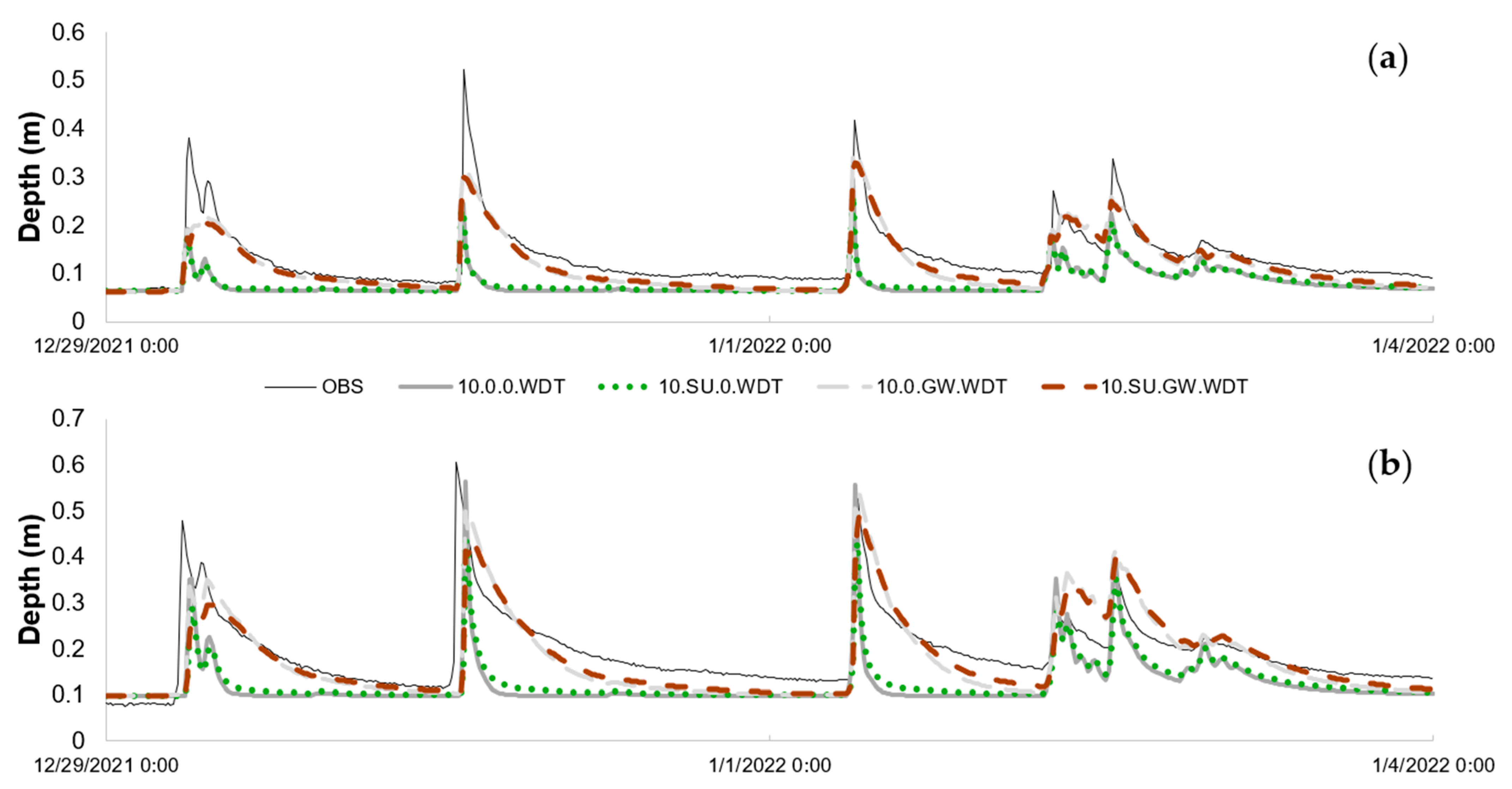
• The fourth and last modeling parameter for SWMM was the inclusion of aquifer components and groundwater–surface water interactions. It was previously observed [48] that accounting for groundwater did improve the overall accuracy of hydrograph drawdown curves compared to earlier results from [35] which neglected groundwater and that a single aquifer approach was valid for this scenario. This sensitivity analysis included groundwater as a parameter to investigate how it interacts with other physical characteristics of the watershed model. The representation of groundwater interflow is governed by Equation (1) [8]:

Q_GW = A1 (H_GW − H*)^B1 − A2 (H_SW − H*)^B2 + A3 (H_GW H_SW),

(1)

where Q_GW is groundwater interflow (m³ s⁻¹ ha⁻¹), H_GW is the initial elevation of groundwater (m), H_SW is the elevation of surface water in the receiving junction (m), H* is the threshold or surface elevation (m), A1 and B1 are the groundwater coefficient and exponent, A2 and B2 are the surface water coefficient and exponent, and A3 is the surface–groundwater interaction coefficient. The coefficients and exponents have no real-world correlation and were calibrated using SRTC assuming uniformity of the aquifer across the watershed. The surface elevation of subcatchments was set to 0.1 m above the rim elevation of the receiving junction to ensure infiltration of rainfall and exfiltration of groundwater. The initial groundwater elevation was set equal to the invert elevation of the receiving node to represent a pre-wetted soil condition. For subcatchments draining into storage basins, this was set equal to the surface elevation to ensure water was present in the basins at the start of the simulation. Other aquifer and groundwater parameters are included in

Table 3. Aquifer and groundwater parameters for sub-watershed.

Aquifer Component	Units	Value	Range
Porosity [49]	-	0.473	0.396–0.487
Wilting point [50]	-	0.167	0.063–0.198
Field capacity [50]	-	0.253	0.160–0.280
Conductivity [50]	mm/h	56.4	33–236
Conductivity slope [8]	-	40.2	40–44
Tension slope	-	15	-
Upper evaporation fraction	-	0.4	-
Lower evaporation depth	m	2	-
Lower groundwater loss rate [51]	mm/h	0.014	-
Initial unsaturated zone moisture content	-	0.3	-
Subcatchment Groundwater Components		Value
A1		0.368
B1		0.976
A2		0.862
B2		3.22
A3		0

. The listed aquifer properties are the spatially weighted averages of external data ranges.

It should be noted that evapotranspiration was considered negligible for this study. The dataset used for the calibration of this model was collected during the winter months where the recorded average daily temperatures ranged from 9 to 13 degrees Celsius [35]. The 30-year average evaporation rate in this part of Alabama was between 5 and 10 mm/month, or less than 0.4 mm/day [52].

There were sixteen model scenarios tested for this study. The modeling parameters considered for each combination are presented in

Table 4. Description and characteristics of SWMM scenarios.

Scenario Name	Subcatchment Delineation Area	Storage (SU)	Groundwater (GW)	Flow Length
10.0.0.WDT	10 ha	Off	Off	WDT
10.0.0.150	10 ha	Off	Off	Max 150 m
10.0.GW.WDT	10 ha	Off	On	WDT
10.0.GW.150	10 ha	Off	On	Max 150 m
10.SU.0.WDT	10 ha	On	Off	WDT
10.SU.0.150	10 ha	On	Off	Max 150 m
10.SU.GW.WDT	10 ha	On	On	WDT
10.SU.GW.150	10 ha	On	On	Max 150 m
5.0.0.WDT	5 ha	Off	Off	WDT
5.0.0.150	5 ha	Off	Off	Max 150 m
5.0.GW.WDT	5 ha	Off	On	WDT
5.0.GW.150	5 ha	Off	On	Max 150 m
5.SU.0.WDT	5 ha	On	Off	WDT
5.SU.0.150	5 ha	On	Off	Max 150 m
5.SU.GW.WDT	5 ha	On	On	WDT
5.SU.GW.150	5 ha	On	On	Max 150 m

. The routing errors across all models were relatively low, ranging from −0.4% to +0.3%.

2.3. HEC-RAS Implementation

For this study, a HEC-RAS 2D with rain-on-grid (RoG) model was developed using version 6.3.1. A 2D grid model divides the terrain into small computational elements called grid cells. Each cell is assigned elevation data; hydraulic properties, such as Manning’s roughness coefficient; impervious percentage; and infiltration capacity from the underlying DEM, land cover, and soil layer [7].

To set up the HEC-RAS 2D RoG model, the same DEM, land cover, and soil data used in the SWMM were imported through RAS Mapper. The study area was then discretized into grid cells of 30 m × 30 m, which was selected to match the CN grid cell size set in SWMM, which in turn conformed to the NLCD [44]. However, the mesh was further refined at critical locations, like river centerlines, riverbanks, road embankments, lake boundaries, and other high or low areas, using break lines and refinement regions of sizes varying from 2 m to 20 m. An important distinction between the HEC-RAS and SWMM is that the former did not have an aquifer component, so the infiltrated water effectively disappears from the simulation. Also, unlike SWMM, the infiltration algorithm in HEC-RAS 2D is designed for event-based hydrological simulation and is not adapted to represent extended period hydrological simulations.

Manning roughness values and impervious percentages were assigned to each land cover type based on recommended values from [7,53]. The infiltration layer was created using the Soil Conservation Survey CN Method by integrating NLCD land cover [44] and SSURGO soil data [45], with CN values adopted in accordance with the one generated by [43] as in SWMM. Figure 2 shows the different types of distributions relative to a portion of a CN grid map.

One external boundary condition at the watershed outlet and two internal boundary conditions were defined. For external boundary conditions, normal depth was set with a friction slope value assigned using the measurement tool in RASMapper near the watershed outlet. The internal boundary conditions were assigned a constant flow hydrograph using values based on StreamStats “Low Flow Statistics” for the watershed [40]. Precipitation time series from [35] observed in the field were uniformly distributed in each grid cell throughout the 2D subbasin area by creating an unsteady flow file.

The HEC-RAS provides four equations for 2D analysis: Diffusion Wave Equation, Shallow Water Equations with a Eulerian–Lagrangian approach (SWE-ELM, Original/Faster), Shallow Water Equation using a Eulerian Approach (SWE-EM, Stricter Momentum), and Shallow Water Equation with Local Inertia Approximation (SWE-LIA, Local Inertia). This study used the Shallow Water Equation (Original/Faster) to run the model for accuracy and to capture the complex scenario. The computational time step was approximated using the Courant–Friedrichs–Lewy Condition. A maximum Courant number of 1, minimum Courant number of 0.02, and a computational time step of 1 s were used. HEC-RAS required significant amounts of time to complete simulations for a weeklong period, ranging from approximately 24 h to run on a computer with an AMD Ryzen 9 processor and 16 GB of RAM, 37 h with an Intel Xeon E-2276M CPU and 32 GB of RAM, and 45 h with an 11th generation i3 processor and 8 GB of RAM. Comparatively, the SWMM completed simulations within a few minutes on an i7 CPU with 12 GB of RAM.

Calibration efforts include changing Mannings’s roughness, culvert dimensions, and underlying terrain. Manning’s roughness values were calibrated along the river channel to match the observed stage and velocity at monitoring stations. Detailed culvert dimensions were unavailable, so they were assigned and calibrated based on the field estimates. Culverts were created using the 2D connection in the geometric editor window for the flow that passes the I-85 road and through the lakes. Whereas for other roads, to represent the culverts and bridges and adjust parts retaining water unrealistically, the terrain was burned-in using the “Terrain Modification Tool”.

Whereas in the SWMM modeling parameters were used to assess the impact they had on the hydrological results, there were two parameters that were used in HEC-RAS RoG modeling efforts, presented in

Table 5. Description and characteristics of HEC-RAS model scenarios.

Scenario Name	Mesh Size	Infiltration Layer	Antecedent Moisture Condition
RAS 1.1	30 m	On	AMC II
RAS 1.2	30 m	On	AMC III
RAS 1.3	30 m	Off	-
RAS 2.1	60 m	On	AMC II
RAS 2.2	60 m	On	AMC III
RAS 2.3	60 m	Off	-

:

• The first was the effect of the average grid cell size for the overland flows, which was either 30 m or 60 m. These do not correspond to the cells that were refined to represent the stream channels, culverts, and other conveyance.
• The second was the effect of infiltration, with three conditions considered: (1) disabling infiltration, (2) normal antecedent moisture conditions (i.e., AMC CN_II), and (3) wet antecedent moisture conditions (AMC CN_III), as shown in Table 5. For the wet soil condition scenario (AMC _III), CN _III was derived from CN _II (Average Runoff Potential, AMC _II) using Table 4.2 from [54].

2.4. Analysis

Several model results were considered to analyze the effects of model parameters. Results were generated for a week-long series of rain events from 29 December 2021 to 4 January 2022. Hydrographs were created for depth and velocity to compare with the measured depth hydrographs and velocity hydrographs calculated from the measured depth with the head-velocity curve for each respective station. Error metrics were calculated from the differences between observed and simulated hydrographs and compiled into tables to evaluate how well each scenario represented real stream data. Flow hydrographs were also generated and used to calculate the total inflow volume for both stations. Total outflow volume was derived for the time series and normalized against the rainfall volume to calculate the runoff coefficient of the watersheds.

Results from each scenario were also compared to each other and to a baseline to evaluate the effects of each parameter and how they interacted with each other in combination. For SWMM, the baseline scenario represented the simplest model parameter option of the four sensitivity analysis parameters:

• Larger default subcatchment delineation area of 10 ha;
• No explicit representation of intermittent storage objects (SUs);
• No groundwater or aquifer object (GW);
• Overland flow width calculated by the WDT.

• For HEC-RAS, the baseline scenario corresponded to the conditions in which calibration was developed, using a computational mesh size of 30 m × 30 m and an infiltration layer with the CN corresponding to AMC II.

This study utilized several error metrics by which model results were compared to collected stream depth data and predicted velocity data calculated from head-velocity curves. These included Nash–Sutcliffe Efficiency (NSE), coefficient of determination (R²), and Root Mean Square Error (RMSE). NSE equally weighs error over the entire simulation period and makes it good for determining overall performance. It is evaluated on a scale from −∞ to 1, where a model is considered more accurate the closer the NSE is to 1. NSE was calculated using Equation (2):

$$\mathrm{N}\mathrm{S}\mathrm{E}=1-{\displaystyle \frac{\sum ({\mathrm{S}\mathrm{I}\mathrm{M}}_{\mathrm{i}}-{\mathrm{O}\mathrm{B}\mathrm{S}}_{\mathrm{i}})}{\sum ({\mathrm{O}\mathrm{B}\mathrm{S}}_{\mathrm{i}}-{\mathrm{O}\mathrm{B}\mathrm{S}}_{\mathrm{m}})}},$$

(2)

where SIM_i is the modeled value at a time step, OBS_i is the observed value at a time step, and OBS_m is the mean of observed values for the whole time series.

R² is a direct comparison of model results to observations on a scale from 0 to 1, where 1 represents a perfect representation. This can be visualized with scatter plots where the model results are treated as a dependent variable of real-world data. These plots can feature a line to show perfect representation to indicate where and to what degree a model may be over- or underestimating. R² was calculated with Equation (3):

$${\mathrm{R}}^2=1-{\displaystyle \frac{\mathrm{R}\mathrm{S}\mathrm{S}}{\mathrm{T}\mathrm{S}\mathrm{S}}},$$

(3)

where RSS is the residual sum of squares and TSS is the total sum of squares.

RMSE is like NSE but weighs larger errors more heavily than smaller errors like standard deviation. This metric was selected as it was believed to be more suitable for determining the accuracy of the recession curves where larger differences were more likely to occur between the model and observations and thus create a larger overall error. A larger RMSE indicates a less accurate model. The equation for RMSE (Equation (4)) is:

$$\mathrm{R}\mathrm{M}\mathrm{S}\mathrm{E}=\sqrt{{\displaystyle \frac{\sum {({\mathrm{S}\mathrm{I}\mathrm{M}}_{\mathrm{i}}-{\mathrm{O}\mathrm{B}\mathrm{S}}_{\mathrm{i}})}^2}{\mathrm{N}}}}$$

(4)

where SIM_i is the modeled value at a time step, OBS_i is the observed value at a time step, and N is the total number of data points.

3. Results

3.1. Subcatchment Overland Flow Length

The overland flow length was one of the least impactful factors on the overall accuracy of the modeled hydrographs compared to observations.

Table 6. Comparison of depth error for scenarios with 10 ha subcatchment discretization area for Capps Way (CAP) and Hamilton (HAM) monitoring sites.

Scenario	NSE		R2		RMSE
	CAP	HAM	CAP	HAM	CAP	HAM
10.0.0.WDT	−0.37	−0.50	0.39	0.29	1.30	1.77
10.0.0.150	−0.38	−0.55	0.37	0.27	1.31	1.80
10.0.GW.WDT	0.74	0.46	0.82	0.65	0.54	0.88
10.0.GW.150	0.73	0.45	0.81	0.65	0.55	0.91
10.SU.0.WDT	−0.32	−0.29	0.41	0.38	1.24	1.62
10.SU.0.150	−0.31	−0.32	0.39	0.36	1.25	1.64
10.SU.GW.WDT	0.75	0.51	0.82	0.62	0.48	0.77
10.SU.GW.150	0.74	0.49	0.81	0.63	0.51	0.81

shows that setting a maximum flow length generally decreased the accuracy in terms of errors compared to scenarios that used the default WDT flow length, with the NSE and R² decreasing and the RMSE increasing. The biggest differences come from scenarios that neglect groundwater, which can be observed in the hydrographs in Figure 3. Those that included groundwater often showed no change in NSE or the R². As is discussed further below, GW was the most impactful parameter.

This negligible effect is visualized in Figure 3, where the hydrographs for comparable scenarios almost match perfectly. It is only in the last rain event that scenarios with the default flow length had slightly slower drawdowns because of the longer period of rainfall. This was true even when the groundwater outflow is accounted for.

Figure 4 compares the inflow at the target junction and the total runoff and exfiltration of the upstream subcatchments. The baseflows were accounted for separately as a constant due to their origination being at a junction and not in a subcatchment. It should be noted that the sum of the flows did not equal the total inflow at the monitoring junctions. The average difference was approximately 2% for Capps Way and 5% for Hamilton bridge. This may be due to a combination of factors, such as the lower groundwater loss when the SWMM aquifer object is present, storage within the conduits and junctions, moisture loss from the drying time parameter, or routing errors, though the routing errors are relatively small as previously mentioned.

The total runoff slightly increased when the flow length cap was applied. Scenarios with groundwater revealed that this coincided with a decrease in exfiltration, which was to be expected as short flow lengths reduce opportunities for runoff to infiltrate. The total outflow and the sum of the inflows were slightly higher for scenarios with a shorter flow length and no groundwater, but approximately the same when groundwater was included, which demonstrates the significance of groundwater to the mass balance.

3.2. Representation of Surface Storage

Table 6 shows that accounting for storage in this watershed had a greater effect on the hydrograph accuracy when groundwater was not accounted for and was more impactful on the accuracy of hydrographs at Hamilton bridge. The differences between the hydrographs are still difficult to discern in Figure 5. The drawdown following the third rain event is obviously slower when storage is included in a groundwater scenario, as would be anticipated. Storage basins, as expected, delay the runoff from upstream subcatchments from reaching the downstream monitoring junctions and create a slower drawdown. Surface storage reduced the peak depths by about 20% without groundwater and 10% when groundwater was considered.

When combined with groundwater, runoff increases and infiltration decreases compared to a scenario without surface storage, as shown in Figure 4. This is likely related to the calibration of subcatchments that drain into the storage which assume a saturated state that does not allow for infiltration or interflow. This results in some of the subcatchments only producing runoff and no exfiltration.

3.3. Spatial Discretization of Subcatchments

Table 7. Comparison of velocity error for different subcatchment delineation size.

Scenario	NSE		R2		RMSE
	CAP	HAM	CAP	HAM	CAP	HAM
10.0.0.WDT	−0.19	0.12	0.38	0.23	9.58	0.95
5.0.0.WDT	−0.25	0.06	0.40	0.23	10.00	1.08
10.0.GW.WDT	0.72	0.32	0.80	0.40	4.47	0.77
5.0.GW.WDT	0.75	0.33	0.78	0.46	4.02	0.86
10.SU.0.WDT	−0.11	0.09	0.40	0.27	8.96	1.09
5.SU.0.WDT	−0.21	−0.02	0.39	0.23	9.54	1.23
10.SU.GW.WDT	0.76	0.39	0.80	0.44	3.88	0.77
5.SU.GW.WDT	0.76	0.34	0.78	0.46	3.54	0.89

compares the velocity hydrograph accuracy for similar scenarios with different subcatchment densities. The results indicate that this is not a significant factor, as the differences between the error metrics are generally relatively small. Comparing the velocity hydrographs in Figure 6 shows a significant overlap of results, just as in Figure 3.

Figure 7 compares the inflow, runoff, and infiltration tied to the monitoring junctions. The average difference between these is about 2–5% of the total volume across all scenarios, with the smaller subcatchments producing slightly less runoff and having more infiltration. This difference could be attributable to differences in the impervious percentage. It can be observed that several scenarios using the 5 ha delineation area have slightly more groundwater exfiltration than scenarios using the 10 ha delineation area. The finer division of subcatchments likely caused some subcatchments to have a lower CN and therefore higher infiltration capacity.

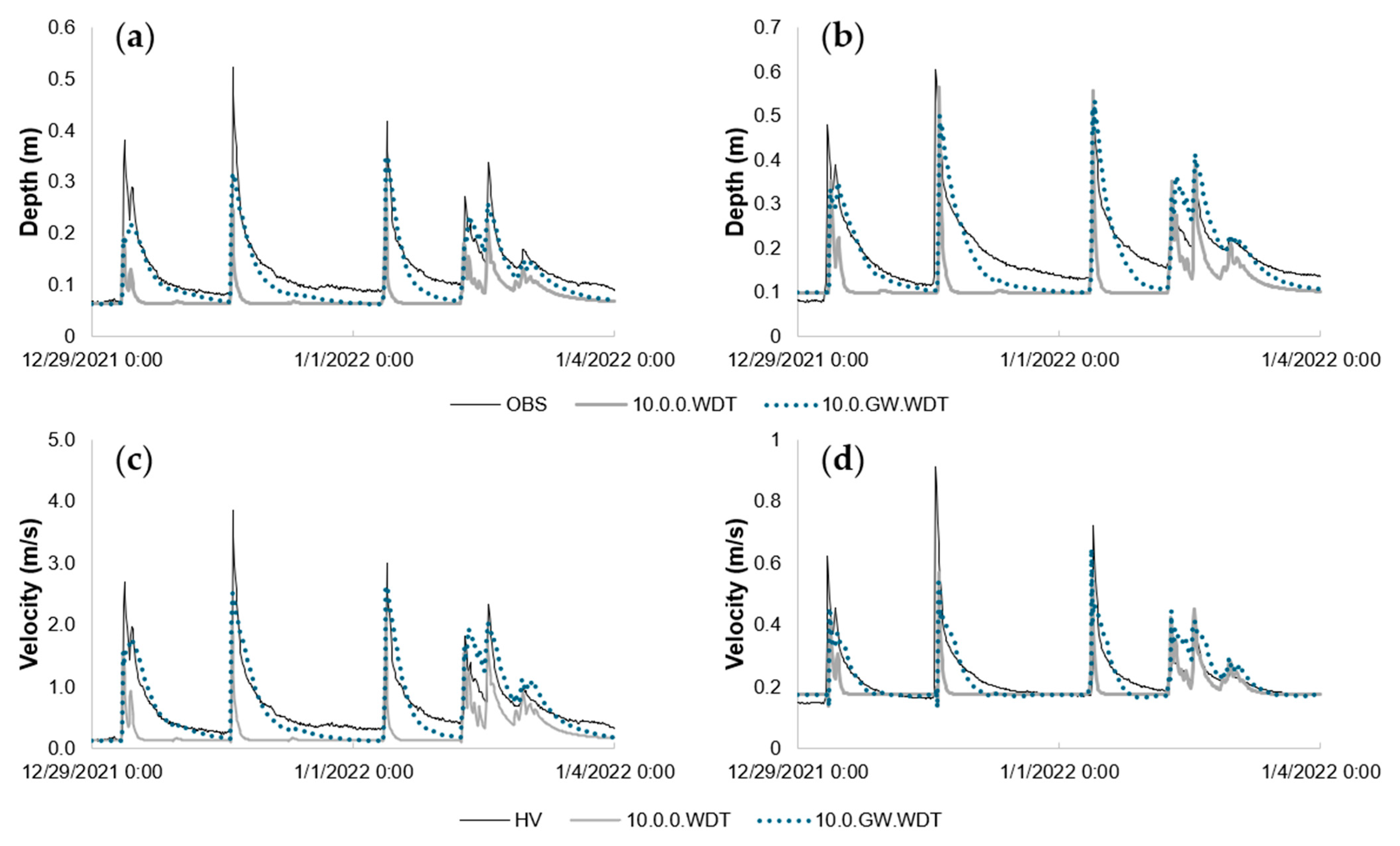
3.4. Aquifer and Groundwater

Groundwater was the most significant factor for hydrograph accuracy. Adding this parameter alone created significant increases to the NSE and R² and decreases in the RMSE in terms of depth, as shown in Table 6. Table 7 also shows improvements in terms of velocity, particularly at the Capps Way junction. There is a noticeable difference in the drawdown phase of hydrographs when comparing non-groundwater and groundwater scenarios. Figure 8 shows that the groundwater scenario had a better representation of the depth and velocity hydrographs. The cause of this is the exfiltration from the aquifer, which occurs over a longer period as water levels in the receiving junctions drop below the water table in the subcatchment. Figure 4 and Figure 7 show that this accounts for about two-thirds of the total inflow at the monitoring junctions.

A sample comparison of the total exfiltration hydrographs across all subcatchments is shown in Figure 9. Certain rain events have a negative outflow at the beginning of rain events. This occurs when surface water from the junction infiltrates into the subcatchment and might be due to the runoff reaching the junction before infiltration has recharged the aquifer. As previously mentioned, models with a finer spatial discretization tended to have more exfiltration than corresponding coarse models. This difference is concentrated around the peak flow rates and is more significant for models with surface storage. This is attributed to the finer models distributing more subcatchments upstream of the storage, which results in a larger area that is undersaturated and able to discharge groundwater.

3.5. Comparison of HEC-RAS Scenarios

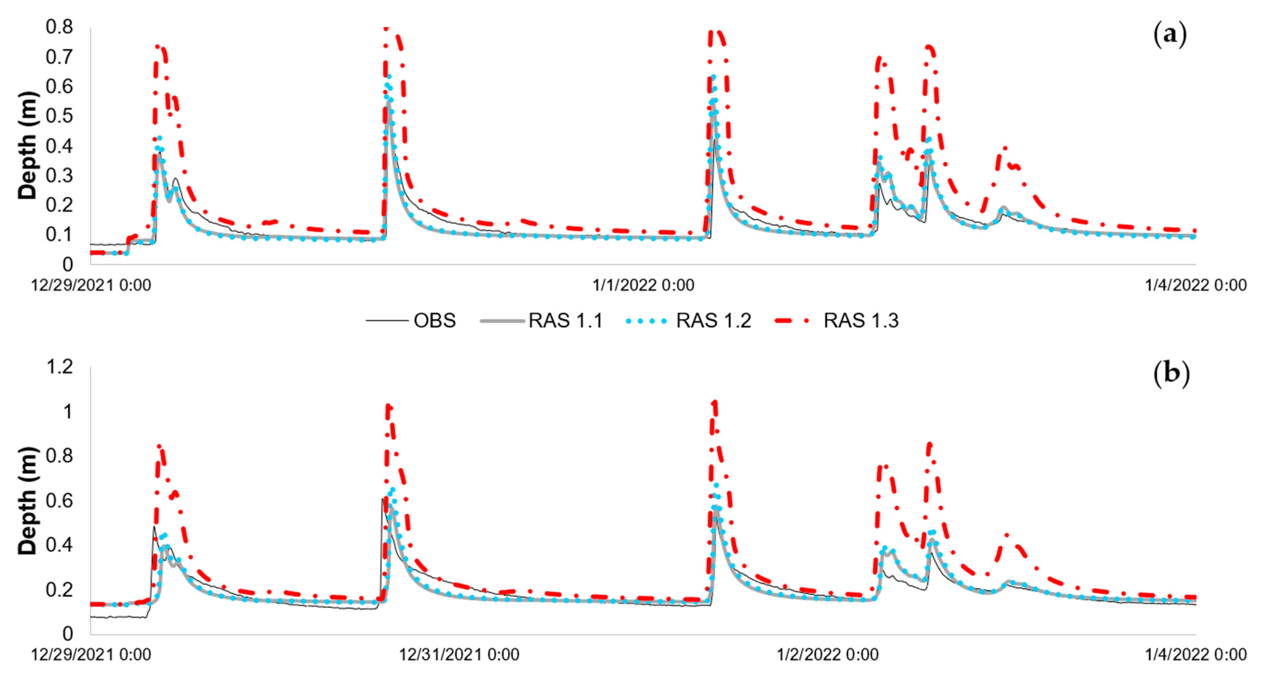
3.5.1. Infiltration

In the HEC-RAS 2D simulation, infiltration played a significant role in shaping the hydrograph. The baseline scenario with normal moisture conditions (AMCII) agreed with the observed peak depths for the first few durations but overestimated during extended rainfall, as shown in Figure 10. The simulated hydrograph’s recession limb was also steeper than that of the observed depth hydrograph. These discrepancies can be attributed to the Curve Number method, which does not consider time-varying infiltration, and the absence of a groundwater component in the HEC-RAS model, which prevents infiltrated water from routing back to the surface as groundwater discharge, contributing to a prolonged recession. When the infiltration was disabled, the surface water depth increased significantly compared to the baseline, with a CN corresponding to AMCII. The peak depth increment was about 78% on average at Capps Way and 96% on average at Hamilton bridge. The peak appeared slightly earlier, and the drawdown rate was steeper than the baseline. This is likely due to all the rainfall becoming runoff immediately without infiltrating into the ground and quickly flowing to the stream. However, when the soil was wet, this increment was approximately 15% and 12% on average at Capps Way and Hamilton bridge, respectively, and no noticeable change was observed in the drawdown rate. This slight increase can be attributable to the higher CN decreasing the infiltration, while still allowing for runoff to occur, with no effect on the modeled drawdown curve.

Similar results can be seen for the stream velocity at these junctions in Figure 11. The difference among the three scenarios, baseline (AMC_II), AMC_III, and no infiltration, is less pronounced at Capps Way than at Hamilton bridge. This outcome can be attributed to the more developed land cover upstream of Capps Way, which already has higher Curve Number values under the baseline (AMC_II) condition. Moreover, accurately representing the channel cross-sections and refining Manning’s roughness coefficients along the channel was crucial during the velocity calibration process over other parameters like the culvert dimensions and the overland’s Manning roughness.

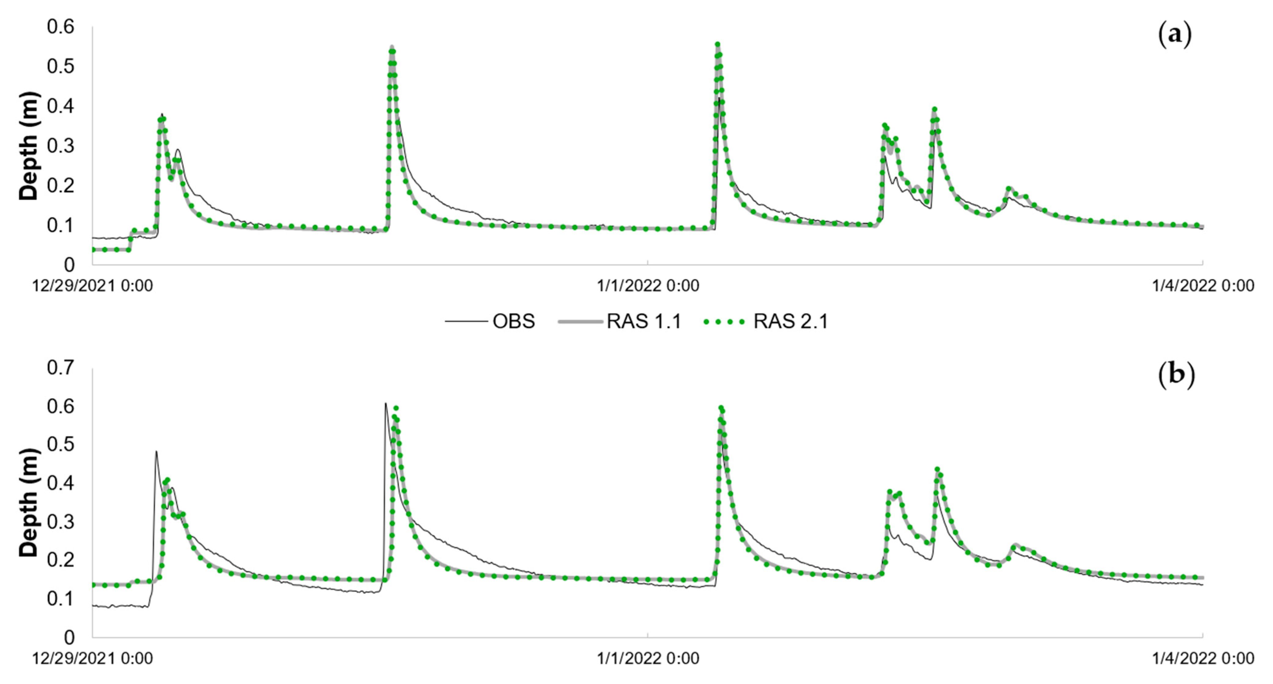
3.5.2. Spatial Discretization of Grid Cells

The results in Figure 12 showed that the finer or coarse grid had an almost negligible effect on the results. This indicates that the coarser grid size was adequate for modeling purposes. At this scale, the grid resolution was not a significant factor for hydrograph accuracy.

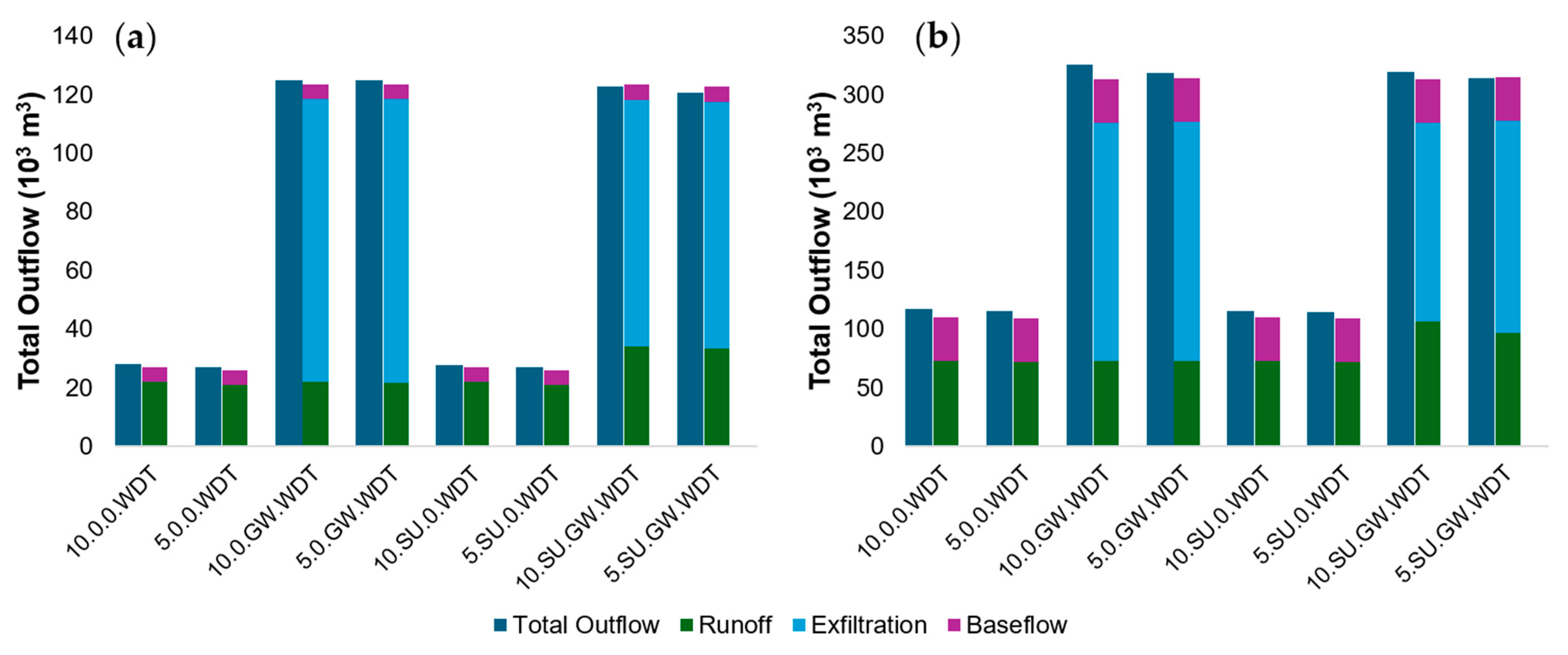
3.6. Comparison of Cumulative Junction Outflow

Figure 13 compares the cumulative junction outflow from either Capps Way or Hamilton bridge across several HEC-RAS and SWMM scenarios. These results should behave distinctively given the different approaches between the selected SWMM and HEC-RAS models.

• The SWMM simulations that do not consider groundwater and aquifers, as well as RAS 1.1 and 1.2, will only consider infiltration for runoff calculations, after which it will no longer be considered.
• The HEC-RAS model that does not consider infiltration (i.e., RAS 1.3) will have most of the rainfall converted to surface runoff. The only abstraction will be depression storage, though there will be no infiltration. These models will generate the most runoff.
• The SWMM simulations that consider the aquifer component will also have an increased runoff, though not as large as RAS 1.3, as a portion of the infiltrated water will enter the subsurface compartment and exfiltrate back into surface junctions as the runoff recedes.

Indeed, when the accumulated runoff is plotted over time, different groupings can be observed from these data. The lowest grouping comprises the baseline SMWM scenario with and without storage present and the HEC-RAS scenarios where infiltration is enabled. These models are the most comparable in terms of modeling capabilities and results, as both neglect to account for the groundwater interflow. The highest grouping consists of the SWMM scenario with storage and groundwater and the RAS scenario with infiltration disabled. These two are comparable in terms of magnitude but utilize different hydrological mechanisms to achieve similar results.

It can be observed in Figure 13 that scenario 10.SU.GW.WDT has a much smoother cumulative curve than any of the other scenarios, including those using the SWMM. This is a result of the groundwater outflow which occurs more gradually than the overland flow. The HEC-RAS scenarios that considered infiltration consistently estimated slightly higher flow rates than the comparable SWMM simulations. Part of this difference can be attributed to the differences in the impervious percentage. The average for all SMWM subcatchments is about 17%, calculated using the cutoff method, while the average for the HEC-RAS was 18.5%, calculated directly from NLCD tables.

Figure 14 compares the resulting hydrographs from this flow at Capps Way. RAS 1.1 and 10.SU.GW.WDT are the closest model comparisons between the two hydrographs in terms of shape. The SWMM baseline does not effectively compare to any of the other scenarios, even though it should be analogous to RAS 1.1 in terms of setup. This is likely a result of differences between the cross-sections across the models, where the flow was more channelized in the HEC-RAS model. The HEC-RAS models used a continuous mesh derived from the DEM that provides detailed elevation data to create a spatially distributed grid, whereas the SWMM simulations used transects taken at discrete points along a conduit to create an average cross-section. Figure 14 also shows the difference in the hydrological behavior between SWMM 10.SU.GW.WDT and RAS 1.3, where RAS1.3 has significantly larger depth peaks resulting from the larger quantity of runoff. The shape of the late drawdown is likely a result of the magnitude of the runoff and the cross-section at this part of the mesh.

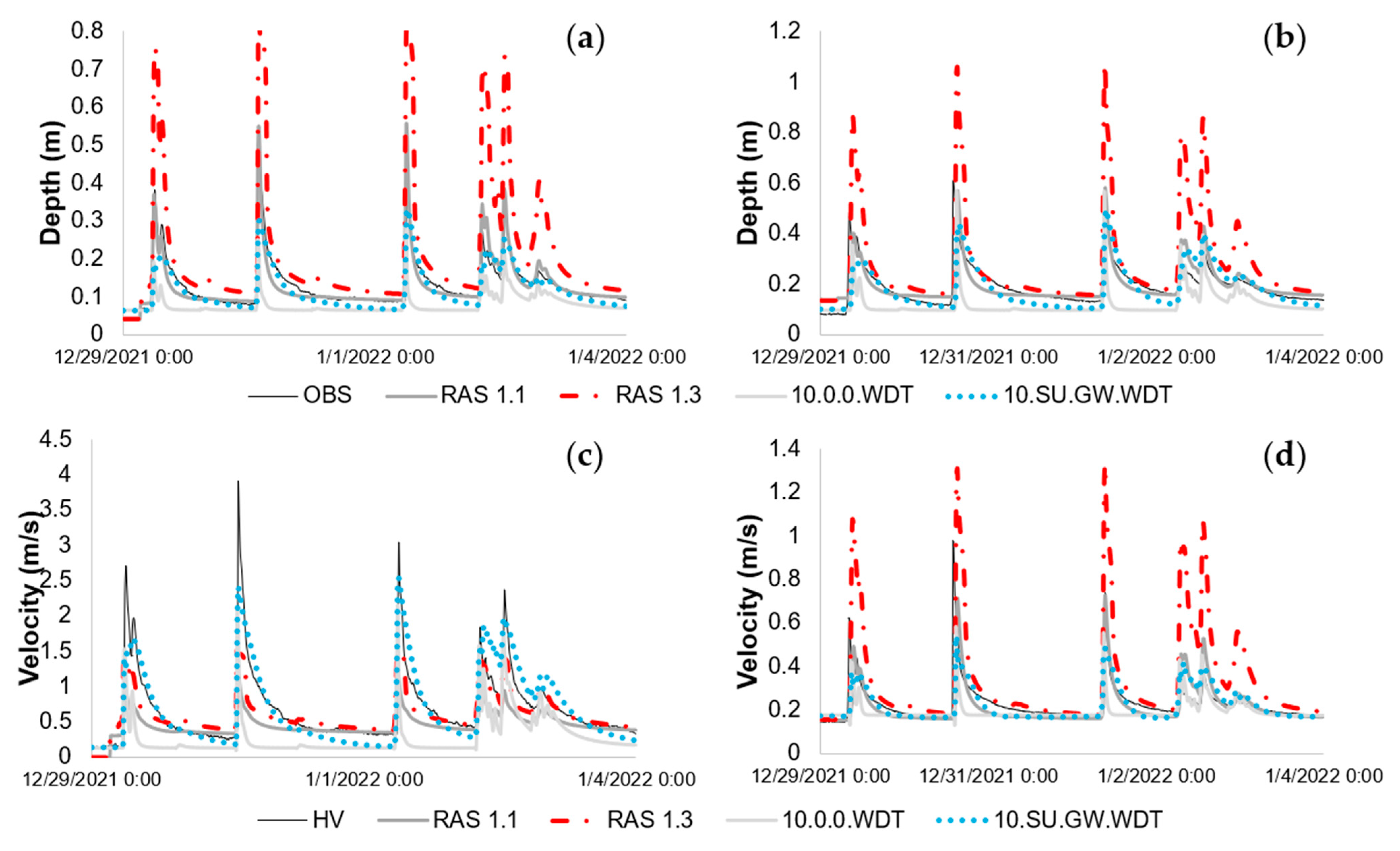
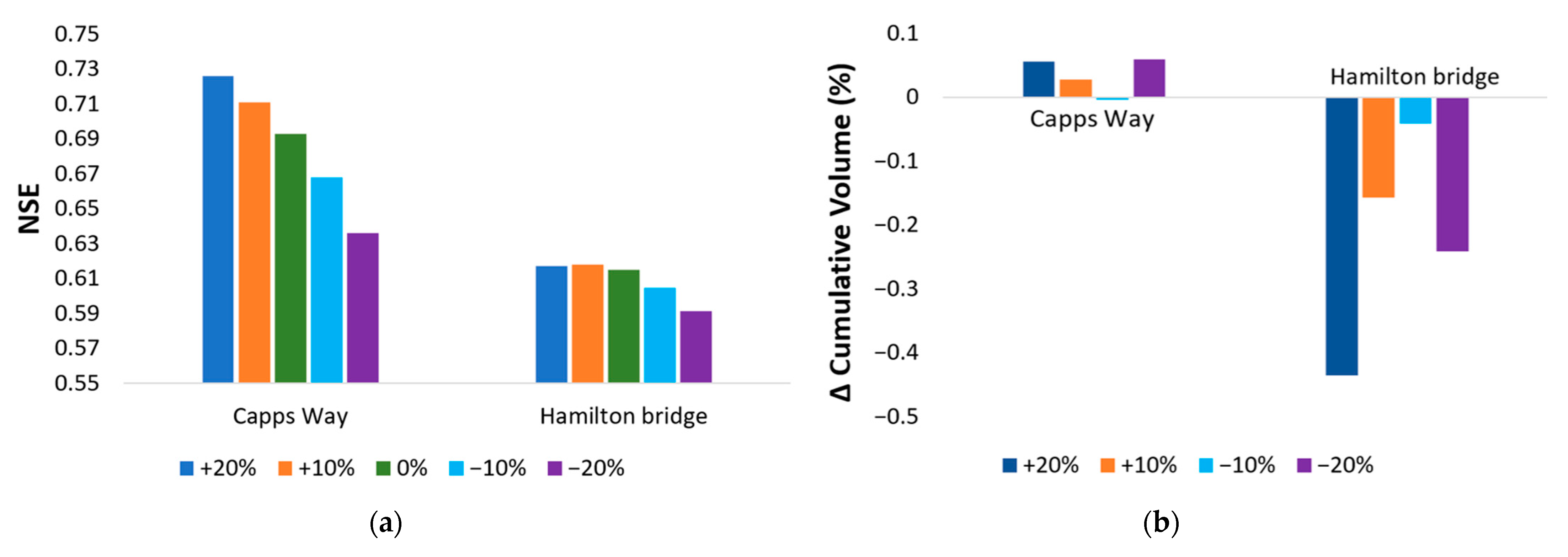
3.7. Sensitivity Analysis

Groundwater and infiltration were demonstrated to be the most significant parameters for the model results. Figure 15 is included below to show the relative insensitivity of some of the other modeling parameters in the SWMM, including the subcatchment slope, Manning’s roughness for impervious (N Imp) and pervious (N Perv) surfaces, and the depression storage for impervious (Dstor Imp) and pervious (Dstor Perv) surfaces. This was achieved using the scenarios 10.SU.0.WDT and 10.SU.GW.WDT. The range of variance is relatively narrow for both locations. Hamilton bridge is shown to be more sensitive than Capps Way, likely due to the larger area with a greater variety of land uses.

Compared to the SWMM, the HEC-RAS was more sensitive to Manning’s roughness value, as shown in Figure 16a. This might be due to the HEC-RAS simulating a spatially distributed overland flow with explicit surface hydraulics. Furthermore, the spatially detailed computational grid in the HEC-RAS leads to localized variations in depth, and roughness changes at such small spatial scales can directly alter flow patterns affecting depth outputs. However, no significant difference was seen in the cumulative runoff volume when changing the Manning’s roughness value.

4. Discussion and Research Limitations

4.1. Discussion

The SWMM reference manuals mention that the overland flow length is important when representing the true sheet flow and maximizing the potential subcatchment infiltration [8]. Most subcatchments had flow lengths larger than 150 m, yet the difference between the total flows of scenarios with and without a flow length cap was almost negligible. Sheet flow may be a more appropriate assumption for developed areas with higher percentages of impervious surfaces and lower infiltration capacities [55] than for natural landscapes that are more permeable and topographically varied. This may be a better assumption to make for less discretized models to account for lower orders of stream [26] without explicitly representing them through conduits. It is believed that the SWMM is limited to representing only sheet flow, regardless of flow length. Alternatively, the flow length calculated with the WDT may have been so long for some subcatchments as to create a longer time of concentration even if the runoff was represented as a rivulet flow.

The representation of surface storage in this watershed did not have as significant an effect on the accuracy and shape of the hydrographs as was initially predicted. This is attributed to both the location of the ponds and where the measurements were taken. Figure 1 shows that most of the surface storage in this watershed is at or near the most upstream part of their respective branches of the stream and were several hundred meters to over a kilometer upstream from monitoring stations. The quantity of runoff entering downstream of these water bodies was significant enough to mitigate their effects on flow rates. Locations closer to storage outlets, as were previously evaluated [35,48], would be more sensitive to changes.

The spatial discretization of the subcatchments and grid cells was another parameter that had minor effects on the model accuracy, which was consistent with previous findings [17,20,24,25]. The dual-scale effect of [17] on the peak flow, whereby aggregation caused larger rain events to have smaller peak flows and smaller events to have larger peaks, was not observed in the SWMM, seen in Figure 6, but was somewhat present in the HEC-RAS, seen in Figure 12. The flow balance is most like those for the small storm in [17], with little difference between the predicted runoff or infiltration. The effects of spatial discretization in this study may be due to the elevation-based delineation of subcatchments and cells. At least in the SWMM this would lead to dissimilar land uses and soil groups being lumped together and skew hydrological parameters like infiltration. However, studies in more uniform watersheds [19,20] showed little difference between runoff calculations, though the relative quantity of runoff was much smaller due to the scale of the study area.

Groundwater was the most significant parameter for hydrograph accuracy. The preceding study [48] was designed to improve upon the representation of hydrograph recession curves by [35] through the inclusion of a groundwater component. The current study further improved upon both studies by developing a better understanding of the SWMM groundwater mechanics. The elevation difference between the receiving node and subcatchment surface was identified as a limiting factor to the earlier research [48] due to it being too small and effectively making all surfaces impervious. This partially accounted for a flawed comparison between the SWMM simulation with groundwater and HEC-RAS models without groundwater, which led to the inclusion of spatial discretization as a parameter for comparison.

This was an important consideration for subcatchments with a surface reservoir as a receiving node since a water table that was too low to begin with would require a significant warm-up period to fill the aquifer. This resulted in these subcatchments tending to have slightly more runoff when groundwater was accounted for, as the high water table limited the potential infiltration. A potential solution for this may be creating a subcatchment that represents the area of the basin, as performed in [26], though this would require assuming no groundwater flow between the subcatchments.

The coefficients and exponents of the groundwater equation are subject to equifinality or the principle of different starting conditions producing similar results, given the arbitrary nature of these variables. Many other calibrations were possible for this model that would have resulted in similar or more accurate hydrographs. One of the limitations of this study is the lack of a comprehensive dataset for subsurface conditions, including groundwater transport, soil conductivity, and water table variations across the watershed.

Infiltration was the most sensitive parameter in the HEC-RAS modeling. Transitioning from normal moisture conditions (AMC II) to wet soil conditions (AMC III) and no infiltration condition significantly increased the runoff depth, which is consistent with earlier findings [56]. However, areas characterized by inherently high Curve Numbers, indicative of extensive impervious surfaces, exhibited minimal sensitivity to further reductions in the infiltration capacity.

The SWMM and HEC-RAS can theoretically produce similar modeling results, but certain calibrations are not truly comparable. SWMM simulations that do not account for groundwater are the most analogous to the HEC-RAS in terms of the outflow quantity because both consider infiltration only for runoff calculations. This infiltrated stormwater is then effectively lost from the system for modeling purposes. The differences in the hydrograph results, as seen in Figure 14, mainly stem from stream cross-sections. Comparison becomes limited when groundwater is introduced to the SWMM as this is a hydrologic feature that the HEC-RAS cannot account for. The surface mesh in the HEC-RAS can be modified to alter how the flow moves through a channel to better match the hydrographs. Infiltration can be modified, as well, to better match the predictions made by the SWMM when the groundwater outflow is accounted for, as in Figure 12. However, these mechanisms require unrealistic modifications of hydrological processes within the watershed. Therefore, SWMM calibrations that use groundwater and aquifer components are not truly comparable to HEC-RAS models. The HEC-RAS has hydrological capabilities, but it is not a complete hydrological model like the SWMM.

The relative insensitivity of the subcatchment slope, Manning’s roughness, and depression storage could indicate a decreasing importance of these factors to model results as the study area increases in size. This was similarly observed in [26] for the conduit roughness, where the significance of this parameter decreased as smaller streams were absorbed into the subcatchment runoff calculations. These factors should not, however, be neglected during calibration, as the findings of this study and [26] only indicate that generalized or aggregated parameters are adequate for models with a coarser spatial discretization. As previously stated, the SWMM was much less sensitive to changes in overland flow parameters compared to the HEC-RAS. The SWMM, being a semi-distributed model, lumps overland flow characteristics and calculations, whereas the HEC-RAS using the full shallow water equations, considering topography derived slopes and cell specific Mannings’s roughness values, more thoroughly distributes these. Only Manning’s values could be compared between the models due to the HEC-RAS using a mesh based on the DEM, which would automatically account for some depression storage and slope. Additionally, the fully distributed HEC-RAS does not differentiate between pervious and impervious Manning’s numbers since the cells are assumed to be small enough to be relatively uniform in terms of land use, whereas the SWMM subcatchments can comprise multiple land use types, which is accounted for with the “% Impervious” parameter.

4.2. Limitations

There are several limitations to this study that future studies can improve upon, field data collection being one of them. Depth logger readings can drift with temperature changes, as observed in [42]. Stilling wells to mitigate other sources of error, as recommended in [36], could not be performed for this research due to resource limitations. The AV sensor was vulnerable to environmental conditions, such as sediment accumulation or low turbidity, that created numerous erroneous readings, particularly at Capps Way. This limited the useful range of more recent head-velocity data for hindcasting velocity hydrographs. The calibration based on these hydrographs is therefore limited in terms of the achievable accuracy relative to both what was measured and what could have been measured with additional resources to limit equipment error.

This study relied on a 1 m × 1 m LiDAR map for elevation data, including most of the stream cross-sections, floodplains, and surface storage geometry. This DEM lacked bathymetry which limited the accuracy of the water body geometry below the water surface. It is not expected that the surface storage geometry would have a significant effect on the hydrograph accuracy as it is not expected that the water level would fluctuate much over time. The accuracy of the depth and velocity hydrographs would, however, be affected by the stream cross-section. Rough surveying was performed to approximate the true cross-section where measurements were taken in the field and used in place of DEM cross-sections. Cross-sections for hydraulic structures, like weirs and orifices for surface storage or culverts, had to be estimated based on the DEM or satellite imagery from [41] because they were generally located on private property and were therefore inaccessible.

As previously stated, many of the aquifer and groundwater parameters were based on external sources and were assumed to be uniform across the watershed. There was no field data collection for hydrologic soil properties or water table changes to verify the available data. Such characterization of the watershed was beyond the scope of this research but is a limitation of the groundwater calibration in this model. Many subsurface properties and behaviors do not directly translate to the SWMM aquifer and groundwater parameters. It was noted by [57] that the SWMM simplifies the groundwater hydrology, including Richard’s equation, and is often coupled with more advanced groundwater models, like MODFLOW or HYDRUS, to better represent these processes. It should also be reemphasized that the HEC-RAS lacks groundwater capabilities which limits comparisons with SWMM simulations to those that consider infiltration only for runoff calculations.

5. Conclusions and Recommendations

This study compared the hydrological modeling of the SWMM and HEC-RAS 2D and the effects of different parameters on hydrographs and flow estimates. For the SWMM, the overland flow length was shown to be relatively insignificant to the model accuracy and runoff predictions. Surface storage was more impactful but limited due to the location of reservoirs relative to the monitoring stations. The spatial discretization of subcatchments was insignificant for some of the same reasons as the overland flow length, which is consistent with observations from previous studies. This was also true of the HEC-RAS, where a finer mesh did not result in substantial differences between hydrographs. The most significant parameter was the representation of the subsurface hydrology as this changed the calculations of the runoff and total flow. Different methods were adopted between the two models, as only the SWMM has groundwater capabilities that account for interflow. This limits comparisons between the SWMM and HEC-RAS as the latter is not a complete hydrological model with groundwater. However, when groundwater is not accounted for, the two are comparable in terms of model hydrographs and flow calculations.

Future studies may investigate these parameters in more detail, such as comparing the effects of intermittent and upstream storage or determining if there is a minimum runoff inflow to necessitate the inclusion of storage for accurate hydrographs. Investigating whether using HEC-RAS cross-sections in the SWMM makes the results similar and vice versa would improve upon the methods used in this study. The future stages of the overarching project this research is part of will involve calibrating the model for the measured levels of total suspended solids in the stream. As the HEC-RAS is further developed to include water quality [58], a comparative analysis of water quality modeling between HEC-RAS calibrations, like RAS 1.1 and RAS 1.3, to SWMM calibrations with comparable outflows may be considered for future investigation.

References

1. USGS. Effects of Urban Development on Floods. Available online: https://pubs.usgs.gov/fs/fs07603/ (accessed on 10 February 2025).
2. US EPA. Construction Site Runoff Control Minimum Control Measure. Available online: https://www.epa.gov/system/files/documents/2023-09/EPA-Stormwater-Phase-II-Final-Rule-Factsheet-2.6-Construction-Runoff.pdf (accessed on 10 February 2025).
3. US EPA. Storm Water Management Model (SWMM). Available online: https://www.epa.gov/water-research/storm-water-management-model-swmm#capabilities (accessed on 10 February 2025).
4. Sitterson, J.; Knightes, C.; Parmar, R.; Wolfe, K.; Avant, M.M.B. An Overview of Rainfall-Runoff Model Types; National Exposure Research Laboratory Office of Research and Development U.S. Environmental Protection Agency: Athens, GA, USA, 2017; pp. 16–19. [Google Scholar]
5. National Academies of Sciences, Engineering, and Medicine. Resilient Design with Distributed Rainfall-Runoff Modeling; National Academies Press: Washington, DC, USA, 2023; pp. 8–17. [Google Scholar] [CrossRef]
6. Rossman, L.A.; Simon, M.A. Appendix A: Useful Tables. In Storm Water Management Model User’s Manual Version 5.2; Center for Environmental Solutions and Emergency Response Office of Research and Development U.S. Environmental Protection Agency: Cincinnati, OH, USA, 2022. [Google Scholar]
7. Brunner, G.W. HEC-RAS 2D User’s Manual Version 6.4; Hydrologic Engineering Center U.S. Army Corps of Engineers: Davis, CA, USA, 2023. [Google Scholar]
8. Rossman, L.A.; Huber, W.C. Storm Water Management Model Reference Manual; National Risk Management Laboratory Office of Research and Development U.S. Environmental Protection Agency: Cincinnati, OH, USA, 2016; Volume 1—Hydrology (Revised). [Google Scholar]
9. Niazi, M.; Nietch, C.; Maghrebi, M.; Jackson, N.; Bennett, B.R.; Tryby, M.; Massoudieh, A. Storm Water Management Model: Performance Review and Gap Analysis. J. Sustain. Water Built Environ. 2017, 3, 04017002. [Google Scholar] [CrossRef] [PubMed]
10. Jang, S.; Cho, M.; Yoon, J.; Yoon, Y.; Kim, S.; Kim, G.; Kim, L.; Aksoy, H. Using SWMM as a tool for hydrologic impact assessment. Desalination 2007, 212, 344–356. [Google Scholar] [CrossRef]
11. Jun, S.; Park, J.H.; Lee, W.; Park, C.; Lee, S.; Lee, K.S.; Jeong, G.C. The changes in potential usable water resources by increasing the amount of groundwater use: The case of Gapcheon watershed in Korea. Geosci. J. 2010, 14, 33–39. [Google Scholar] [CrossRef]
12. US Army Corps of Engineers. HEC Newsletter—Spring 2016: Advances in Hydrologic Engineering. Available online: https://www.hec.usace.army.mil/newsletters/HEC_Newsletter_Spring2016.pdf#:~:text=HEC,capability%20to%20handle%20large%20terrain (accessed on 24 March 2025).
13. Bartles, M.; Brauer, T.; Ho, D.; Fleming, M.; Karlovits, G.; Pak, J.; Van, N.; Willis, J. Hydrological Modeling System HEC-HMS User’s Manual; Hydrologic Engineering Center Institute for Water Resources U.S. Army Corps of Engineers: Davis, CA, USA. Available online: https://www.hec.usace.army.mil/confluence/hmsdocs/hmsum/latest (accessed on 20 March 2025).
14. James, W. Optimal Model Complexity. In Rules for Responsible Modeling, 4th ed.; Computational Hydraulics International: Guelph, ON, Canada, 2005; pp. 61–71. [Google Scholar]
15. Warwick, J.J.; Tadepalli, T. Efficacy of SWMM Application. J. Water Resour. Plann. Manag. 1991, 117, 352–366. [Google Scholar] [CrossRef]
16. Snikitha, S.; Kumar, G.P.; Dwarakish, G.S. A Comprehensive Review of Cutting-Edge Flood Modelling Approaches for Urban Flood Resilience Enhancement. Water Conserv. Sci. Eng. 2024, 10, 2. [Google Scholar] [CrossRef]
17. Ghosh, I.; Hellweger, F.L. Effects of Spatial Resolution in Urban Hydrologic Simulations. J. Hydrol. Eng. 2011, 17, 129–137. [Google Scholar] [CrossRef]
18. Zarriello, P.J.; Barlow, L.K. Measured and Simulated Runoff to the Lower Charles River, Massachusetts, October 1999–September 2000; U.S. Geological Survey: Northborough, MA, USA, 2002. [Google Scholar]
19. Goldstein, A.; Foti, R.; Montalta, F. Effects of Spatial Resolution in Modeling Stormwater Runoff for an Urban Block. J. Hydrol. Eng. 2016, 21, 06016009. [Google Scholar] [CrossRef]
20. Shaneyfelt, K.M.; Johnson, J.P.; Hunt, W.F. Hydrologic Modeling of Distributed Stormwater Control Measure Retrofit and Examination of Impact on Subcatchment Discretization in PCSWMM. J. Sustain. Water Built Environ. 2021, 7, 04021008. [Google Scholar] [CrossRef]
21. Kim, B.; Sanders, B.F.; Schubert, J.E.; Famiglietti, J.S. Mesh type tradeoffs in 2D hydrodynamic modeling of flooding with a Godunov-based flow solver. Adv. Water. Resour. 2014, 68, 42–61. [Google Scholar] [CrossRef]
22. David, A.; Schmalz, B. A Systematic Analysis of the Interaction between Rain-on-Grid-Simulations and Spatial Resolution in 2D Hydrodynamic Modeling. Water 2021, 13, 2346. [Google Scholar] [CrossRef]
23. Godara, N.; Bruland, O.; Alfredsen, K. Comparison of two hydrodynamic models for their rain-on-grid technique to simulate flash floods in steep catchment. Front. Water 2024, 6, 1384205. [Google Scholar] [CrossRef]
24. Ongdas, N.; Akiyanova, F.; Karakulov, Y.; Muratbayeva, A.; Zinabdin, N. Application of HEC-RAS (2D) for Flood Hazard Maps Gen-eration for Yesil (Ishim) River in Kazakhstan. Water 2020, 12, 2672. [Google Scholar] [CrossRef]
25. Costabile, P.; Costanzo, C.; Ferraro, D.; Macchione, F.; Petaccia, G. Performances of the New HEC-RAS Version 5 for 2-D Hydrodynamic-Based Rainfall-Runoff Simulations at Basin Scale: Comparison with a State-of-the Art Model. Water 2020, 12, 2326. [Google Scholar] [CrossRef]
26. Wanniarachchi, S.S.; Wijesekera, N.T.S. Challenges in field approximations of regional scale hydrology. J. Hydrol. Reg. Stud. 2020, 27, 100647. [Google Scholar] [CrossRef]
27. Ali, S.E. Assessing the Performance of 2D HEC-RAS Rain-on-Grid Model: A Case Study in the Rainbow Creek Subwatershed. Master’s Thesis, The University of Guelph, Guelph, ON, Canada, 2024. Available online: https://hdl.handle.net/10214/28047 (accessed on 20 March 2025).
28. Ennouini, W.; Fenocchi, A.; Petaccia, G.; Persi, E.; Sibilla, S. A complete methodology to assess hydraulic risk in small ungauged catchments based on HEC-RAS 2D Rain-On-Grid simulations. Nat. Hazard. 2024, 120, 7381–7409. [Google Scholar] [CrossRef]
29. James, W.R.C.; Finney, K.; James, W. Auto-Integrating Multiple HEC-RAS Flood-line Models into Catchment-wide SWMM Flood Forecasting Models. AWRA Hydrol. Watershed Manag. Tech. Comm. 2012, 7, 1–15. [Google Scholar]
30. Khalaj, M.R.; Noor, H.; Dastranj, A. Investigation and simulation of flood inundation hazard in urban areas in Iran. Geoenviron. Disasters 2021, 8, 18. [Google Scholar] [CrossRef]
31. Khatooni, K.; Hooshyaripor, F.; Malekmohammadi, B.; Noori, R. A new approach for urban flood risk assessment using coupled SWMM-HEC-RAS-2D model. J. Environ. Manage. 2025, 374, 123849. [Google Scholar] [CrossRef]
32. Barszcz, M.; Bartosik, Z.; Rukść, S.; Batory, J. Comparison of maximum flows calculated in urban catchment using HEC-RAS and SWMM models. Sci. Rev. Eng. Environ. Stud. 2016, 25, 410–424. [Google Scholar]
33. Sun, P.; Wang, S.; Gan, H.; Liu, B.; Jia, L. Application of HEC-RAS for flood forecasting in perched river—A case study of hilly region, China. IOP Conf. Ser. Earth Environ. Sci. 2017, 61, 012067. [Google Scholar] [CrossRef]
34. Bagheri, K.; Requieron, W.; Tavakol, H. A Comparative Study of 2-Dimensional Hydraulic Modeling Software, Case Study: Sorrento Valley, San Diego, California. J. Water Manag. Model. 2020, 28, C471. [Google Scholar] [CrossRef]
35. Xiao, H. Evaluating Alternatives for the implementation of Curve Number in SWMM for an urbanized watershed. Master’s Thesis, Auburn University, Auburn, AL, USA, 2022. [Google Scholar]
36. Onset Computer Corporation. HOBO U20L Water Level Logger (U20L-0x) Manual; Onset Computer Corporation: Bourne, MA, USA, 2024. [Google Scholar]
37. Onset Computer Corporation. HOBO Data Logging Rain Gauge (RG3 and RG3-M) Manual; Onset Computer Corporation: Bourne, MA, USA, 2018. [Google Scholar]
38. Teledyne Isco. 2150 Area Velocity Flow Module and Sensor Installation and Operation Guide; Teledyne Instruments, Inc.: Lincoln, NE, USA, 2024. [Google Scholar]
39. USDA. USDA Geospatial Data Gateway (GDG). Available online: https://datagateway.nrcs.usda.gov/ (accessed on 2 June 2023).
40. USGS. StreamStats. Available online: https://streamstats.usgs.gov/ss/ (accessed on 7 June 2023).
41. City of Auburn. City of Auburn (COA) Map. Available online: https://webgis.auburnalabama.org/coamap/ (accessed on 6 January 2025).
42. Moore, M. Measuring and Modeling Stormwater Runoff from an Interstate in a Rural/Forested Watershed. Ph.D. Thesis, Auburn University, Auburn, AL, USA, 2016. [Google Scholar]
43. Siddiqui, A.R. Curve Number Generator: A QGIS Plugin to Generate Curve Number Layer from Land Use and Soil. 2020. Available online: https://github.com/ar-siddiqui/curve_number_generator (accessed on 2 June 2023).
44. USGS. Annual National Land Cover Database. 2024. Available online: https://www.usgs.gov/centers/eros/science/annual-national-land-cover-database (accessed on 28 February 2025).
45. USDA. Soil Survey Geographic Database (SSURGO). 2024. Available online: https://doi.org/10.15482/USDA.ADC/1242479 (accessed on 28 February 2025).
46. Guo, J.C.; Urbonas, B. Conversion of Natural Watershed to Kinematic Wave Cascading Plane. J. Hydrol. Eng. 2009, 14, 839–846. [Google Scholar] [CrossRef]
47. UDFCD. Chapter 5—Runoff. In Drainage Criteria Manual; Urban Drainage and Flood Control District: Dever, CO, USA, 2007. [Google Scholar]
48. Bragg, M.; Vasconcelos, J. Evaluating the Effects of Groundwater on Runoff Modelling Using PCSWMM. J. Water Manag. Model. 2025; in review. [Google Scholar]
49. USGS. Soil Properties Dataset in the United States. Available online: https://www.sciencebase.gov/catalog/item/5fd7c19cd34e30b9123cb51f (accessed on 9 June 2023).
50. USDA. Web Soil Survey. Available online: https://websoilsurvey.nrcs.usda.gov/app/WebSoilSurvey.aspx (accessed on 9 June 2023).
51. USGS. National Ground-Water Monitoring Network. Available online: https://cida.usgs.gov/ngwmn/index.jsp (accessed on 9 June 2023).
52. NWS. Evaporation Climatology (mm). Available online: https://www.cpc.ncep.noaa.gov/products/Soilmst_Monitoring/US/Evap/Evap_clim.shtml (accessed on 13 February 2025).
53. Chow, V.T. Open Channel Hydraulics; McGraw-Hill: New York, NY, USA, 1959. [Google Scholar]
54. USDA. Section 4: Hydrology. In SCS National Engineering Handbook; Soil Conservation Service, U.S. Department of Agriculture: Washington, DC, USA, 1972; p. 10.7. [Google Scholar]
55. Saghafian, B.; Julien, P.Y. Introduction. In Resistance to Sheet Flow; Hydrological Modeling Group Center for Geosciences Colorado State University: Fort Collins, CO, USA, 1989; pp. 1–2. [Google Scholar]
56. Kim, J.; Johnson, L.; Cifelli, R.; Thorstensen, A.; Chandrasekar, V. Assessment of antecedent moisture condition on flood frequency: An experimental study in Napa River Basin. CA J. Hydrol. Reg. Stud. 2019, 26, 100629. [Google Scholar] [CrossRef]
57. Tu, M.C.; Wadzuk, B.; Traver, R. Methodology to simulate unsaturated zone hydrology in Storm Water Management Model (SWMM) for green infrastructure design and evaluation. PLoS ONE 2020, 15, e0235528. [Google Scholar] [CrossRef]
58. US Army Corps of Engineers. Water Quality. Available online: https://www.hec.usace.army.mil/software/waterquality/ (accessed on 27 March 2025).
Figure 1. MMC stream network in Opelika sub-watershed.
Water 17 01331 g001
Figure 2. Example CN grid distribution for different models: (a) SWMM with subcatchments having average area of 10 ha and (b) HEC-RAS with computational grids with 30 m grid resolution.
Water 17 01331 g002
Figure 3. Comparison of depth hydrographs for scenarios with different overland flow lengths: (a) Capps Way and (b) Hamilton bridge.
Water 17 01331 g003
Figure 4. Comparison of total inflow, runoff, and infiltration for 10 ha subcatchment discretization area: (a) Capps Way and (b) Hamilton bridge.
Water 17 01331 g004
Figure 5. Comparison of depth hydrographs for scenarios with and without surface storage represented: (a) Capps Way and (b) Hamilton bridge.
Water 17 01331 g005
Figure 6. Comparison of velocity hydrographs for scenarios with different subcatchment delineation sizes with head-velocity (HV) hydrograph: (a) Capps Way and (b) Hamilton bridge.
Water 17 01331 g006
Figure 7. Comparison of total inflow, runoff, and infiltration for different subcatchment discretization size: (a) Capps Way and (b) Hamilton bridge.
Water 17 01331 g007
Figure 8. Comparison of model scenarios with and without groundwater to measured depth and head-velocity (HV) hydrographs: (a) Capps Way depth; (b) Hamilton bridge depth; (c) Capps Way velocity; and (d) Hamilton bridge velocity.
Water 17 01331 g008
Figure 9. Comparison of total exfiltration across all subcatchments between models with different spatial discretization: (a) no surface storage and (b) storage.
Water 17 01331 g009
Figure 10. Comparison of depth hydrographs for scenarios with small discretization: (a) Capps Way and (b) Hamilton bridge.
Water 17 01331 g010
Figure 11. Comparison of velocity hydrographs for scenarios with small discretization to head-velocity (HV) hydrograph: (a) Capps Way and (b) Hamilton bridge.
Water 17 01331 g011
Figure 12. Comparison of depth hydrographs with different levels of discretization: (a) Capps Way and (b) Hamilton bridge.
Water 17 01331 g012
Figure 13. Comparison of cumulative inflow volume and runoff coefficients: (a) Capps Way cumulative volume; (b) Hamilton bridge cumulative volume; (c) Capps Way runoff coefficient; and (d) Hamilton bridge runoff coefficient.
Water 17 01331 g013
Figure 14. Comparison of hydrographs between SWMM and HEC-RAS: (a) Capps Way depth; (b) Hamilton bridge depth; (c) Capps Way velocity; and (d) Hamilton velocity.
Water 17 01331 g014
Figure 15. Sensitivity analysis of SWMM simulation 10.SU.GW.WDT’s overland flow parameters relative to observations in terms of NSE: (a) Capps Way and (b) Hamilton bridge.
Water 17 01331 g015
Figure 16. Sensitivity analysis of HEC-RAS model RAS1.1 to Manning’s roughness: (a) depth-based NSE relative to observations and (b) cumulative runoff volume difference relative to baseline simulation (RAS1.1).
Water 17 01331 g016