Article

Turbulent and Subcritical Flows over Macro-Roughness Elements †

by
Francisco Martínez
* and
Javier Farías
School of Civil Engineering, Pontificia Universidad Católica de Valparaíso, Brasil #2147, Office 5-3, Valparaíso 2340000, Chile
*
Author to whom correspondence should be addressed.
This paper is an extended version of our paper published in the “12th International Conference on Fluvial Hydraulics, River Flow 2024”, Liverpool, UK, 2–6 September 2024.
Water 2025, 17(9), 1301; https://doi.org/10.3390/w17091301
Submission received: 11 February 2025 / Revised: 3 April 2025 / Accepted: 5 April 2025 / Published: 27 April 2025
(This article belongs to the Special Issue Open Channel Flows: An Open Topic That Requires Further Exploration)

Abstract

:
Determining the friction coefficients for uniform flows over very rough bottoms is a long-standing problem in open-channel hydraulics and river engineering. This experimental study presents measurements of the surface deformation as well as Darcy–Weisbach and Manning friction coefficients for steady, turbulent (6058 R e 28,502), and subcritical flows (0.14 F r 0.52) over large roughness elements, where F r and R e denote the Froude and Reynolds numbers, respectively. The experiments were conducted in a rectangular, inclined flume with a train of half-cylinders mounted on the bed, with radii in the range 20 mm a 50 mm. These obstacles yield a relative submergence 1.45 h N / a 4.41 and a constant spacing ratio e / a = 12.8 across all experimental runs, where h N and e denote the normal flow depth and the center-to-center spacing between cylinders, respectively. The relative amplitude of the surface profiles, ( Δ h / a ), was analyzed and found to correlate strongly with h N / a , R e and F r . The results reveal very high values of the Darcy friction factor, f, which follows scaling laws of the form f ( h N / a ) n ^ , with n ^ < 0 , independent of a, and f R e β , where β < 0 is closely linked to a. Scaling relationships for the Manning roughness coefficient, (n), were also investigated and are reported herein.

1. Introduction

Free-surface flows over rough and very rough beds are ubiquitous in both natural and industrial contexts. Examples include environmental river floods, fluvial streams over sedimentary bedforms, and flows over large particles such as boulders and rocks [1,2,3,4]. Similar conditions also arise in industrial settings, such as the mining industry, where sedimentary bedforms develop from the movement of solid–liquid suspensions [5], and in the atmospheric boundary layer dynamics around urban structures [6]. In the fluvial context, numerous studies have sought to characterize frictional properties using both numerical and experimental approaches [2,3,7,8,9,10,11,12,13,14,15,16,17,18,19,20]. These studies have consistently identified key hydraulic parameters—such as flow rate (Q), average velocity (V), flow depth (h), and bottom slope (i)—as influential. Nevertheless, despite this progress, the role of roughness size and spatial distribution in shaping flow dynamics remains insufficiently understood and underexplored in the current literature.
This topic was first addressed by Bazin and Darcy [21], who conducted experiments in a large sloped flume in Bourgogne (France), affixing square ribs of height k with regular spacing along the bed. These flows are now known as k-type rough flows [22]. Bazin demonstrated that the Chezy law could be extended to open-channel flows, a formulation now typically expressed in the Darcy–Weisbach form as follows [23,24]:
f = 8 g R i V 2
where i is the bed slope, V is the cross-sectional average velocity, R is the hydraulic radius of the uniform flow, and f is the Darcy friction factor. Following Lim [24], Bazin proposed that f is primarily governed by the relative roughness rather than the slope itself. He also introduced an empirical relationship for the resistance coefficient, applicable for Reynolds numbers in the range 40,000 R e 600,000 . Bazin’s extensive and influential dataset was later used to estimate the Manning roughness coefficient [24].
Davis [25] notes that Morris [26,27] emphasized the significance of the longitudinal spacing e between roughness elements. Chow [23] subsequently classified roughness regimes based on e, as follows: (1) isolated-roughness flow, where element-induced wakes dissipate before reaching subsequent elements; (2) wake-interference flow, where wakes from adjacent elements overlap; and (3) quasi-smooth flow, where closely spaced elements cause the flow to skim their crests, creating dead zones in between (see Figure 1). Chow identified regimes (1) and (2) as the most influential on flow friction and free surface deformation [23]. According to Oke [6,28], these regimes correspond to e / k > 2 , e / k 1 , and e / k < 1 / 2 , respectively.
Morris [26] also highlighted the role of the submergence ratio, Λ = h / k , i.e., in identifying wake-interference flow, particularly in shallow flow regimes. He proposed a critical spacing, ( e c ), to distinguish isolated roughness from wake interference at high Reynolds numbers. Nikora et al. [29] supported Morris’s findings through their studies of fluvial flows over gravel-boulder beds, identifying four hydrodynamic layers influenced by both the local roughness geometry and spatial distribution.
If the arrangement of roughness elements alters local flow structures, then a corresponding impact on global friction characteristics—specifically the Darcy friction factor f—should be expected. In this vein, Bathurst [2] observed that resistance equations become highly inaccurate for shallow flows, where large roughness elements cause significant free surface deformation. Lawrence investigated this link by analyzing overland flow over rough granular surfaces [30] and through experiments on uniform flow over half-sphere roughness elements [31]. He identified the strong dependence of f on Λ , delineating the following three regimes: (i) partial inundation regime ( Λ < 1 ), (ii) marginal inundation ( Λ 1 ), and (iii) well-inundated regime ( Λ 1 ). In the latter two regimes, f may be approximated by the following:
f C Λ 2 , Λ 1
1 f = a + b ln ( Λ ) , Λ 1
where C = 10 , a = 1.22 , and b = 0.883 . The form of Equation (3) resembles the Nikuradse log-law for rough flows [32], which Bayazit [33] also observed in studies of large-scale roughness. Lawrence further identified additional resistance due to the free surface waves generated by roughness protrusions, termed wave resistance. His results validated Bazin’s emphasis on the significance of ( Λ ).
McSherry et al. [34] investigated the transitional effects in k-type rough flows through large-eddy simulations and flume experiments. They reported that the logarithmic velocity layer proposed by Nikora et al. [29] diminishes for low submergence ratios ( Λ > 1 ) and re-emerges at higher values ( Λ 1 ). McSherry also observed weak undular surface jumps, which appeared to influence momentum balance and drag.
Despite these advances, the effect of asperity geometry has received limited attention [35,36]. Forbes [37] studied the flow around a single half-cylinder, showing that surface profiles can be estimated using potential flow theory. Vigie [38] extended this work experimentally, identifying diverse surface deformation patterns and proposing a topological classification governed by the Froude number and parameter Λ , where h is the flow depth and k = a denotes the roughness scale (i.e., cylinder radius).
Among the few studies examining the friction factor in flows over regularly spaced obstacles of various shapes, Ryu et al. [39] found that f is highly sensitive to obstacle geometry. For semi-circular, triangular, square, and dune-shaped ribs, f increased to approximately 0.2 when e / k < 8 but dropped below 0.1 when e / k > 8 (with e defined as the center-to-center spacing).
In light of the above, this study investigates the behavior of classical resistance laws in steady, uniform, subcritical turbulent flows over beds composed of large, half-cylindrical ribs. Special emphasis is placed on the effects of rib spacing e and size a, exploring scaling laws that emerge from the data and their implications for flow hydraulics.

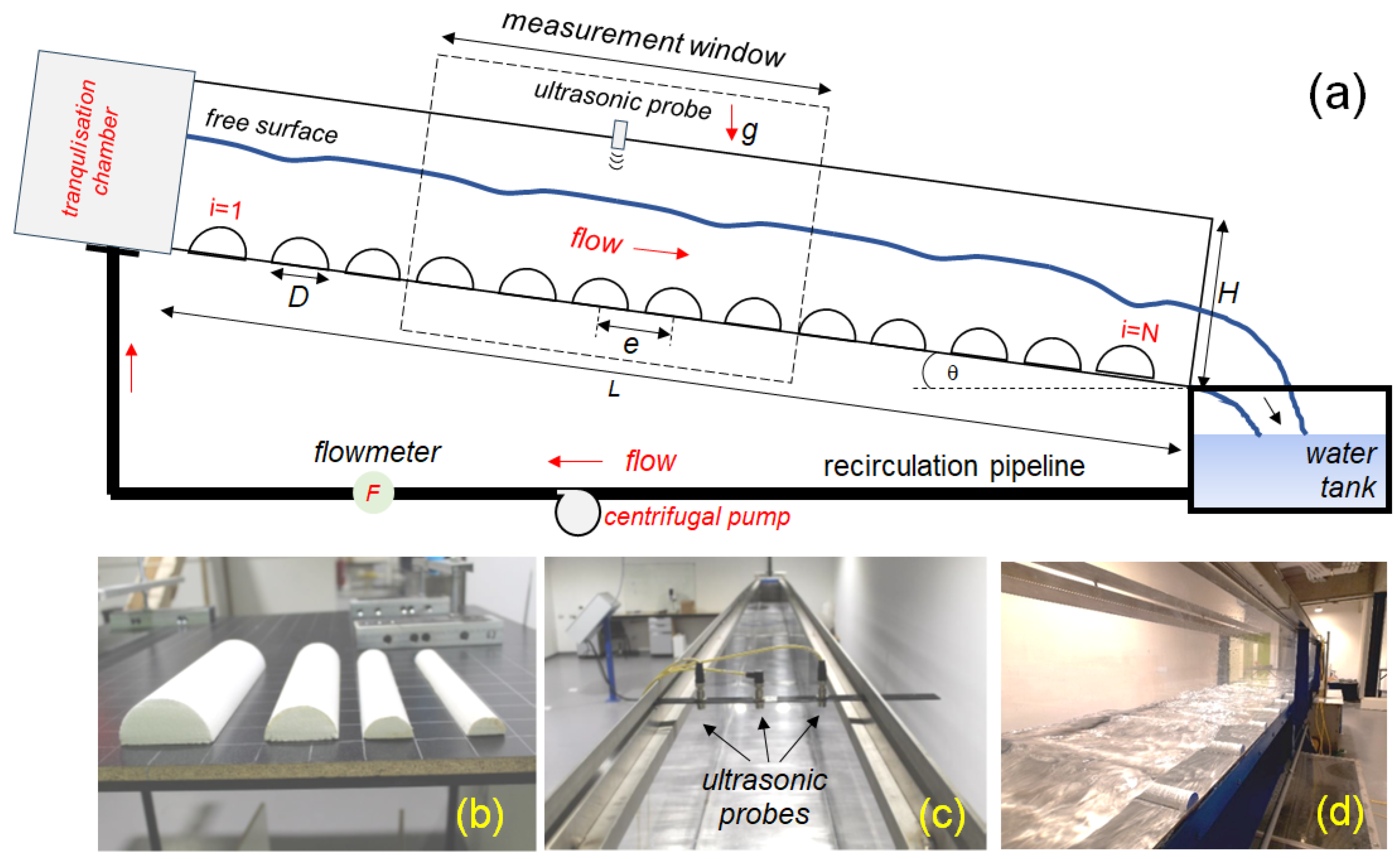
2. Experimental Setup

2.1. Materials

The experiments were conducted in the recirculating flume at the Laboratory of the School of Civil Engineering, Pontificia Universidad Católica de Valparaíso, Chile. The flume had a total length of L = 9.90 m, a rectangular cross-section with width W = 0.358 m, and a total height H = 0.40 m. The bed slope, denoted i = tan ( θ ) , was varied within the range from 0 to 1.50%. The system was supplied by a centrifugal pump, with a variable frequency drive (VFD) regulating the flow rate (Q) in the range from 3 to 15 Ls−1.
The roughness elements consisted of half-cylinders made from high-density Styrofoam, with radii a = D / 2 = 20, 25, 35, and 50 mm. A schematic of the experimental setup is shown in Figure 2a,d. To minimize surface asperities and promote consistent hydrodynamic interaction, the cylinders were coated with a thin layer of waterproof paint.
Flow depth measurements were performed using three ultrasonic sensors (model PICO+100/I, MICROSONIC Co., Biel, Switzerland), which operated simultaneously at a fixed frequency of f = 200 kHz. The sensors were mounted above the flow and provided a measurement precision of approximately 1% of the reading. The flume’s sidewalls, constructed of Plexiglas, allowed for the clear visualization of the flow. High-speed imaging of the free surface was recorded from one side using a camera (model EOS Rebel T6, CANON Inc., Tokyo, Japan) operating at 60 frames per second.

2.2. Methodology

For a given experiment, N, half-cylindrical obstacles of diameter D were placed along the flume bed, spaced at a center-to-center distance e. As many arrays as obstacle diameters were tested during the campaign (cf. Table 1). All arrays were configured such that the aspect ratio ξ = e / D = 12.8 was maintained across all experiments. According to Chow [23] and Oke [6], this configuration corresponds to the isolated-roughness regime, which is known to exert the greatest influence on flow friction.
A central section of the flume, approximately Δ L 6 m in length, was designated for all flow depth measurements. The bed slope was fixed at i = 0.8 % for all experiments. Under these conditions, the flow sufficiently far from the inlet stabilizes into a uniform regime, independent of the inlet and outlet effects. Water enters the flume via a tranquilization chamber that minimizes turbulence at entry. The flow then proceeds freely into the channel and discharges into a collection tank from where it is recirculated, as shown in Figure 2a.
The first cylinder in each array ( i = 1 ) was placed near the flume inlet, and the last one ( i = N ) was positioned 1 cm before the outlet. According to Monin and Yaglom [40], the distance required for the boundary layer to span the flow depth can be estimated using the following:
δ = 0.33 x o u * U
where δ is the boundary layer thickness, x o is the distance from the leading edge, u * = g R i is the friction velocity, and U is the mean velocity, approximated as U = Q / A . Imposing δ = h N , the estimated development length x o falls in the range 0.41 m x o 1.91 m.
Pokrajac et al. [41] performed velocity and depth measurements for subcritical flows over square transverse ribs in a recirculating flume at the University of Aberdeen. Although their obstacle shapes differed, their hydraulic conditions were similar, yielding x o 1.55 , in close agreement with the present study. Thus, for x > x o , the flow can be considered uniform and the turbulent boundary layer fully developed.
Once the flow rate was set, steady-state conditions were reached rapidly. Flow depth measurements were then taken along the central, left, and right axes of the flume. The number of measurement stations M varied with obstacle size, from approximately 53 for a = 50 mm to M 87 for a = 20 mm. Lateral measurements were performed no less than 1 cm from the sidewalls to minimize boundary effects. The instantaneous flow depth h ˜ ( x , t ) was obtained from the following:
h ˜ ( x , t ) = d ( x , t ) s ( x , t )
where s ( x , t ) is the ultrasonic sensor reading, and d = H z ( x ) , with z ( x , t ) denoting the vertical coordinate of the local bed elevation ( z = 0 for flat regions, z > 0 atop a cylinder). Flow depth was recorded for approximately T = 30 s per location, ensuring statistical convergence. Ambient temperature was monitored to limit environmental effects on sensor performance. An Arduino-based system relayed sensor data to a PC for storage. The time-averaged depth at each location was calculated as follows:
h ( x ) = 1 R i = 1 R h ˜ ( x , t i )
where R 2024 is the number of time samples per station.

2.3. Estimation of the Normal Depth of the Flow and Froude and Reynolds Numbers

Using Equation (6), the spatial average flow depth in the region of interest—interpreted as the normal depth h N —was computed as follows:
h N = 1 M k = 1 M h ( x k )
where M is the number of measurement stations (ranging from ∼53 to 87 points). The streamwise average hydraulic radius R and mean flow velocity V were then determined as follows:
R = W h N W + 2 h N
V = Q W h N
The dimensionless Froude and Reynolds numbers—key parameters in free surface flow—were evaluated using the following:
F r = V g h N
R e = V R ν
with ν (= 10 6 m2 s−1) representing the kinematic viscosity of water. Hereafter, Equation (7) is adopted as a reliable estimate of the uniform flow depth h N in each experimental run. The associated standard error is typically within ±1.5. The minimum flow rate tested (Q = 3.0 Ls−1) ensured the full submergence of the obstacles, resulting in h N / a > 1.48 for all cases. The reference normal depth without obstacles, h N 0 , was also recorded under identical conditions and ranged from 15.8 mm to 42.7 mm. According to Chow [23], the laminar-to-turbulent transition in open-channel flow typically occurs within 500 < R e < 2000 , though the upper bound is somewhat arbitrary. For this study, flow is considered turbulent when R e > R e c , where R e c = 2000 is used as a conservative threshold. Overall, the Froude number varied from 0.14 to 0.52, and the Reynolds number from 6058 to 28,502, corresponding to subcritical flows in the turbulent regime.

3. Results and Discussion

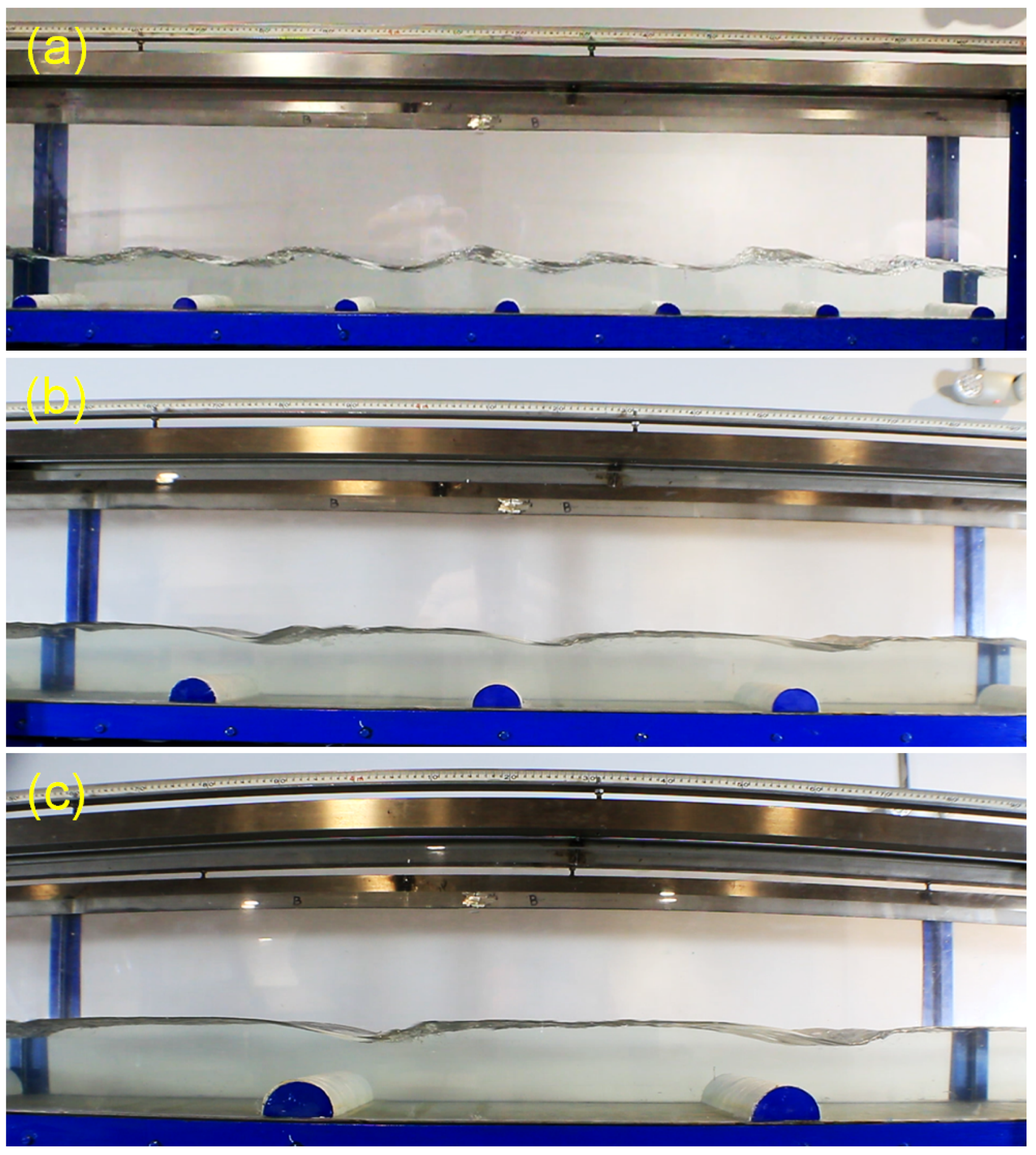
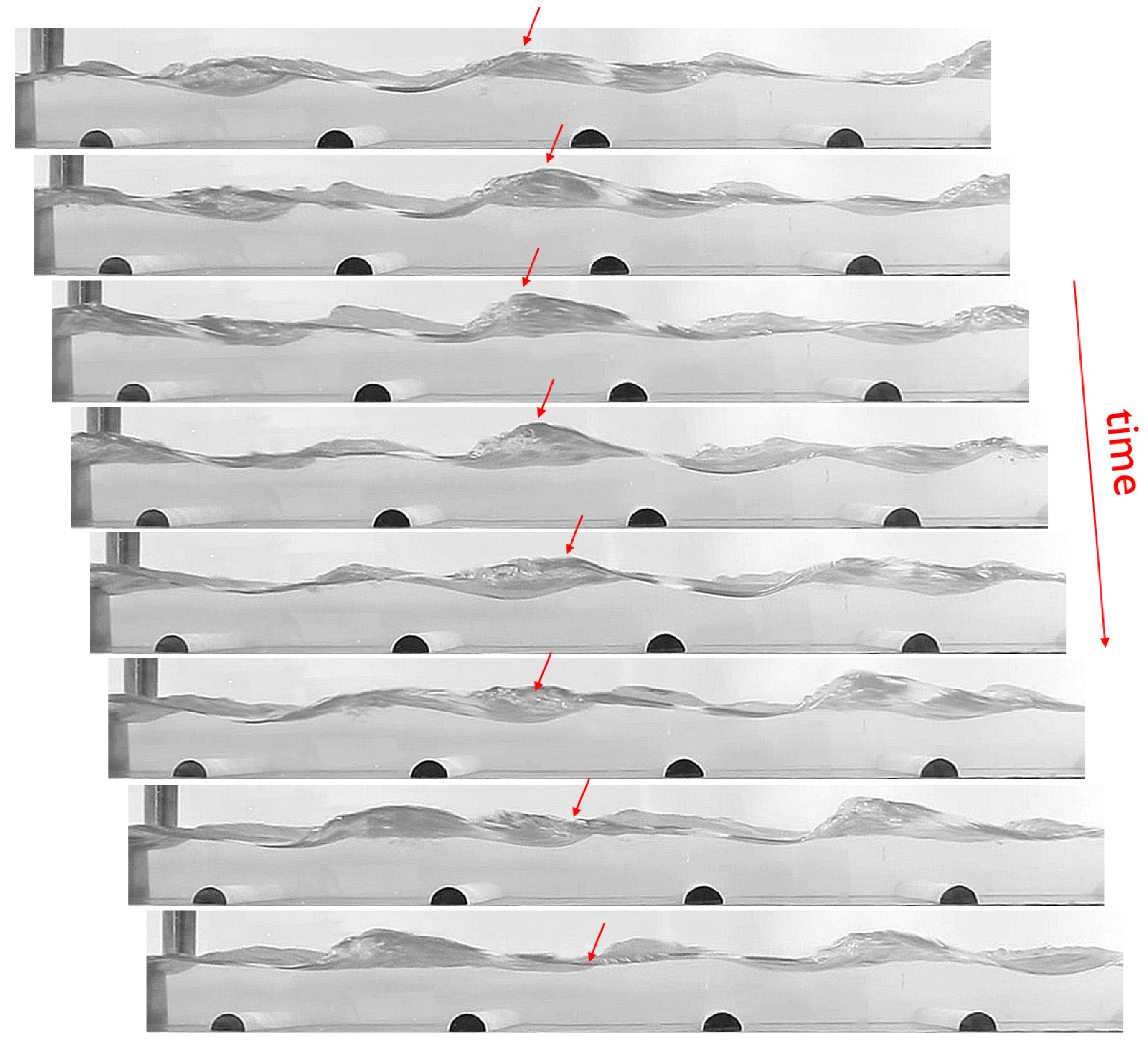
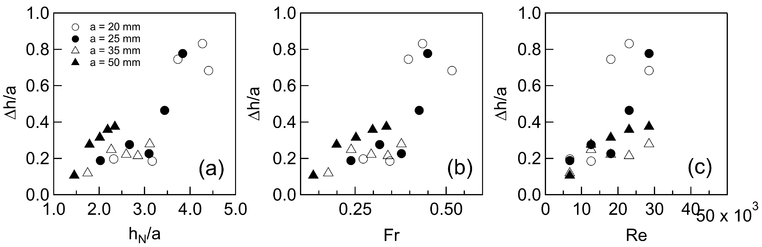
3.1. Deformation of the Free Surface and Backwater Profiles

Figure 3, Figure 4 and Figure 5 illustrate the flow characteristics over the array of half-cylindrical obstacles under varying hydraulic conditions. Figure 3 presents the free surface profiles for obstacles with a radius of a = 25 mm and increasing flow rates. At lower flow rates (Figure 3c), the surface becomes increasingly irregular, with the peaks and valleys shifting positions over time. The amplitude of these surface oscillations ( Δ h ) becomes particularly pronounced at higher discharges. The deformation patterns shown in Figure 3a,b were the most commonly observed across the experimental campaign, regardless of obstacle size or flow rate.
Figure 4 explores the impact of obstacle size on surface deformation at a constant flow rate ( Q = 15 Ls−1). Interestingly, larger obstacles do not necessarily produce greater surface disturbances, as might be expected. On the contrary, the water surface between obstacles recovers its normal depth more rapidly as obstacle size—and hence spacing—increases. Furthermore, a single valley consistently forms between adjacent obstacles, typically closer to the upstream cylinder. For larger radii ( a 35 mm), surface profiles become more stable over time, forming persistent, undular jump-like features whose positions remain nearly fixed.
In contrast, such invariance diminishes with smaller obstacles under high flow conditions. Figure 5 shows the temporal evolution of surface deformation over a 1-s interval for a = 25 mm. Surface peaks migrate upstream and decay in amplitude throughout each cycle (as indicated by the red arrows), while the dynamics of this cycle ( Δ T ) were not statistically analyzed, preliminary observations suggest its structure depends on the flow rate. This temporal variability, especially pronounced with a = 20 and 25 mm, highlights the challenges in characterizing surface wave structures, which appear quasi-stationary only under specific combinations of geometry and turbulence intensity.
Using ultrasonic probe data, the time-averaged free surface profiles h ( x ) were obtained for all configurations. Figure 6 summarizes these profiles across different arrays and flow rates. The normal depth h N from Equation (7) is presented in Figure 6a. All profiles exhibit a periodic bumping structure with alternating peaks and valleys along the analysis window. These bumps are asymmetric, with peak amplitudes typically occurring just downstream of each obstacle—consistent with the observations by Vigie [38] and Lawrence [31], who described similar patterns in experiments involving singular and repeated bottom obstructions. Lawrence termed this surface behavior undular jumps.
The relative amplitude of deformation, h N / a , was computed as the streamwise average of peak-to-valley differences (cf. Figure 6a). Figure 7 illustrates that while Δ h / a correlates well with F r , R e and h N / a , no single empirical law fits all datasets precisely. Nonetheless, a consistent trend is evident: as these parameters increase, so does Δ h / a —though not necessarily Δ h itself— emphasizing the importance of analyzing this phenomenon using relative rather than absolute scales.

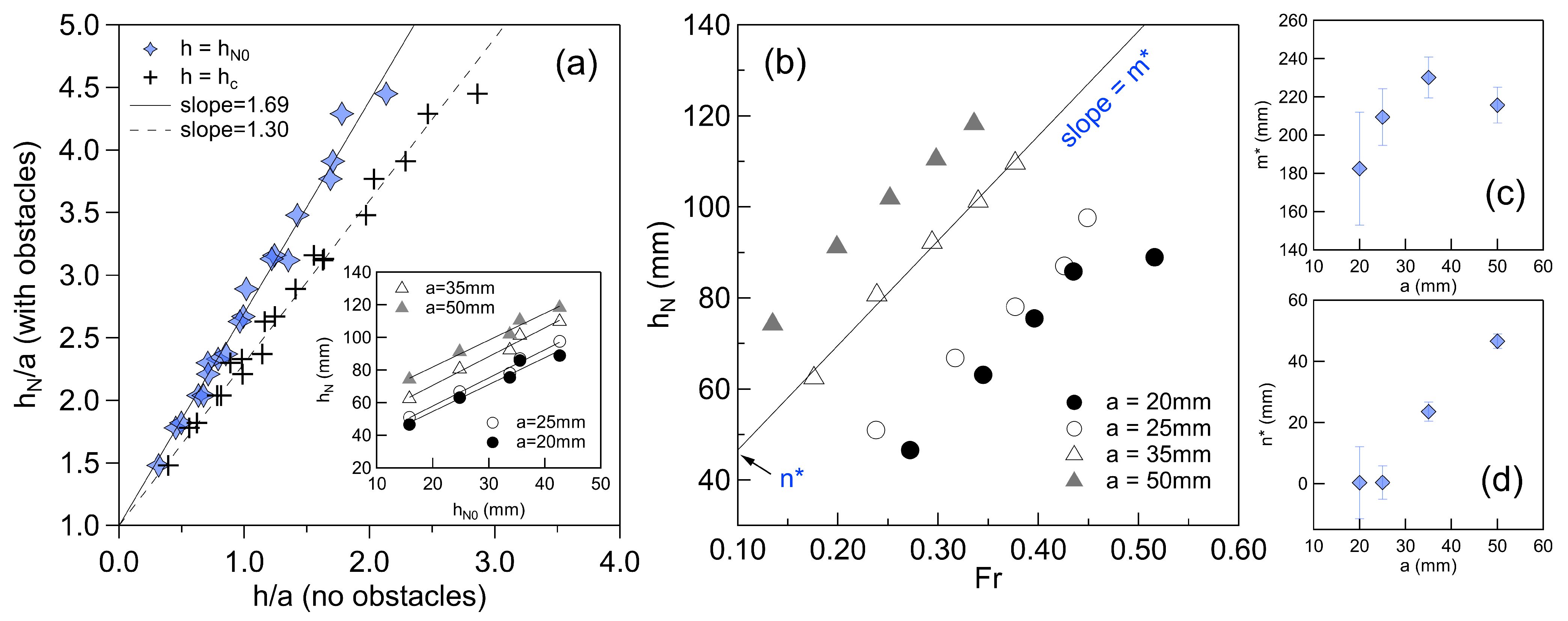
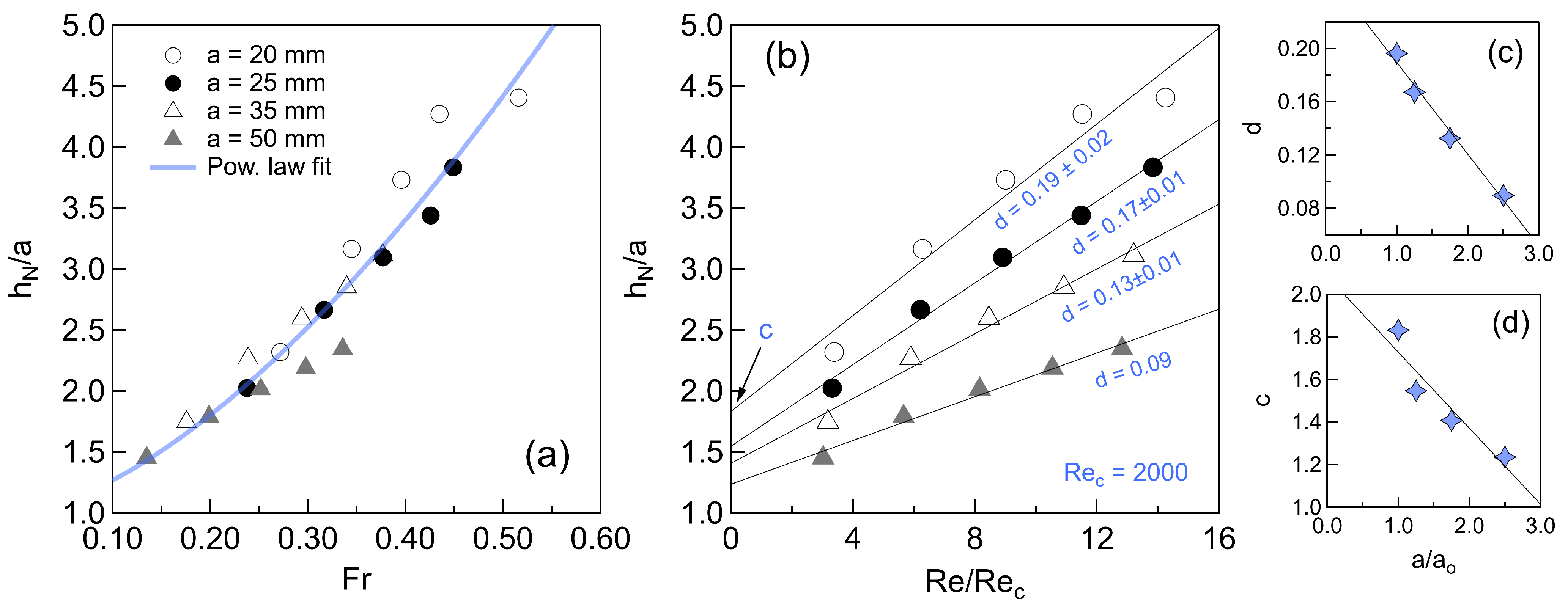
3.2. Distribution of the Normal Depth

The inset of Figure 8a ccompares the measured normal depth over the cylinders ( h N ), with the corresponding depth measured in their absence ( h N 0 ). The data align closely along straight lines whose slopes depend on the cylinder radius a. The main plot in Figure 8a seeks to generalize this observation by comparing the dimensionless normal depth h N / a with h / a , where h may represent either the critical depth h c or the baseline depth h N 0 . The resulting relationship can be described by the empirical function:
h N a = 1 + s h a
where s = 1.69 ± 0.02 when h = h N 0 , and s = 1.30 ± 0.01 when h = h c . The critical depth was computed as h c = q 2 / g 1 / 3 , representing the flow rate per unit width. As expected, Equation (12) confirms that h N h N 0 , and h N h c , highlighting the substantial influence of the cylinders on the flow field.
The inset of Figure 8c,d, yielding the expression:
h N = n * + m * F r
The variation of m * is notably non-linear, with a decreasing trend observed for larger obstacles. This is consistent with the qualitative behaviors discussed in Figure 3 and Figure 4, suggesting that some attenuation mechanism may limit wave amplitude growth as flow interacts with larger cylinders.
Plotting h / a against F r yields the curve shown in Figure 9a, which can be approximated by:
h N a = 1 + r 1 ( F r ) r 2
with r 1 = 10.2 ± 1.2 and r 2 = 1.6 ± 0.1 . The exponent ( r 2 1 ) reflects the non-linear dependence inherited from the behavior of m * , n * .
Figure 9b compares h N / a against the dimensionless Reynolds number R e / R e c , using R e c = 2000 . Four approximately linear trends emerge, each associated with a different obstacle size, and fitted by:
h N a = c + d R e R e c
The fitting parameters c and d are functions of the relative cylinder radius a 0 / a , where a 0 = 20 mm is the smallest obstacle size used as a reference. Their distributions are given by the following:
c = c 1 + c 2 a a o
d = d 1 + d 2 a a o
with fitting constants ( c 1 , c 2 ) = ( 0.3 , 0.1 ) and ( d 1 , d 2 ) = ( 2.1 , 0.4 ) . These relations allow the empirical representation of h N / a in terms of R e and obstacle size.

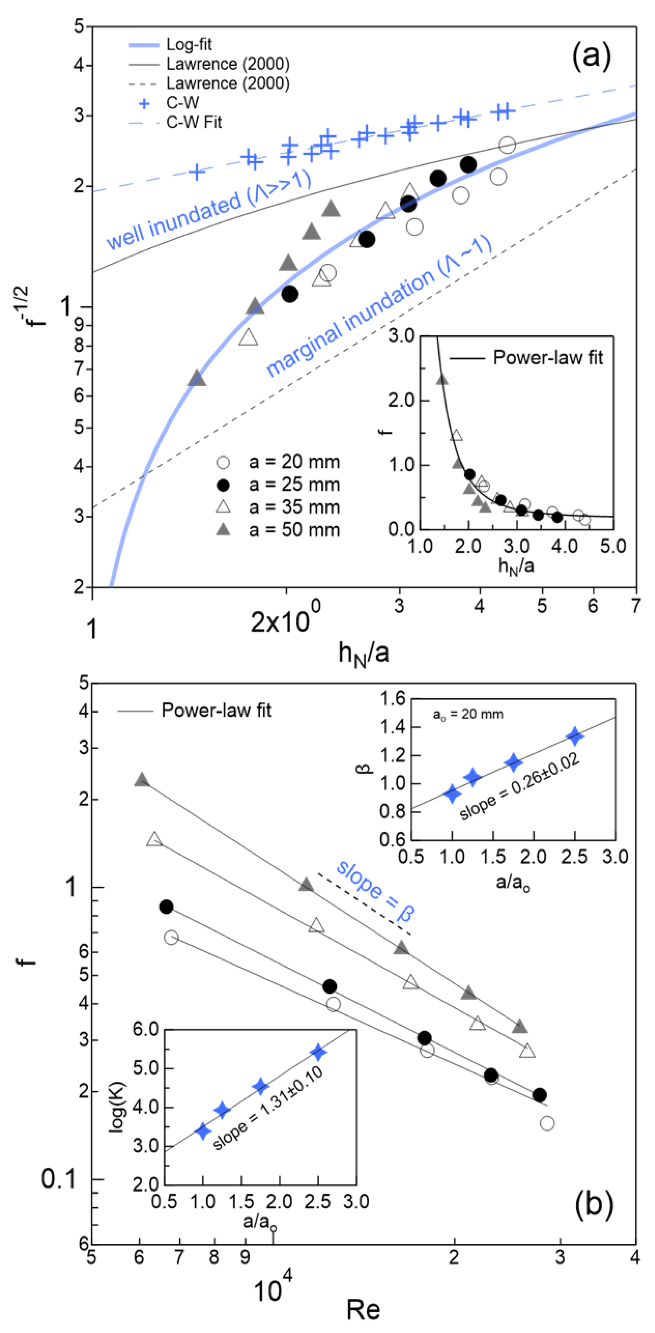
3.3. About the Darcy Friction Coefficient

Figure 10a presents the Darcy–Weisbach friction coefficient f, plotted in the transformed form 1 f against the submergence ratio h N / a for all experiments. The data cluster well around a single curve, represented by the following empirical relation:
1 f = a ^ + b ^ log h N a
with fitting parameters a ^ = 0.10 ± 0.13 and b ^ = 3.5 ± 0.3 . Although Equation (18) resembles formulations previously proposed by Lawrence [31] and Bayazit [33], the present dataset lies between the marginal inundation and well-inundated regime defined by Lawrence. Specifically, the marginal inundation curve underpredicts and the well-inundated regime overpredicts the observed friction.
For comparison, the classical Colebrook–White equation, adapted for open-channel conditions with R e > 3000 , was also applied as follows:
1 f C W + 2 log ε 12 R + 2.51 R e f C W = 0
where ε is the equivalent roughness height, taken here as ε = a , and R is the hydraulic radius. This implicit equation was solved numerically. As shown in Figure 10a, Colebrook–White predictions also overestimate the measured friction values, further emphasizing the uniqueness of the macro-roughness effects captured in this study.
The inset in Figure 10a displays f directly against h N / a , yielding an alternative empirical form as follows:
f = f + m ^ h N a n ^
where m ^ = 9.1 ± 1.6 , n ^ = 3.9 ± 0.4 , and f = 0.19 ± 0.06 represents an asymptotic value for deep flows ( h N / a ). This inverse power-law behavior is consistent with earlier studies by Bathurst [2,8,9], and it underscores the significant energy dissipation caused by the large bottom obstacles. Across all configurations, the friction coefficient ranged from 0.16 to 2.31, indicating intense resistance effects in these macro-roughness regimes.
Figure 10b explores the dependence of f on the Reynolds number R e using a log–log scale. The data exhibit the power-law behavior that can be fitted as follows:
f = K R e β
where K and β are fitting coefficients. This structure echoes similar forms used by Choo et al. [42], and it also resembles the Blasius correlation for pipe flow friction in smooth turbulent regimes [43]. Notably, the empirical coefficients span a wide range as follows: from K = 2474 ± 927 to 262,630 ± 18,500 and from β = 0.93 to 1.34. Both parameters are clearly influenced by the obstacle size, as expressed by the dimensionless ratio a / a o , as shown in the insets of Figure 10b. These relationships are captured by the following empirical expressions:
β = t o + t 1 a a o
log K = p o + p 1 a a o
where t o = 0.69 ± 0.04 , t 1 = 0.26 ± 0.02 , p o = 2.20 ± 0.18 , and p 1 = 1.31 ± 0 . 10. These scaling laws further confirm the close interdependence between frictional behavior, obstacle geometry, and flow regime.
Figure 10. Distribution of the Darcy friction factor (f) for all the experiments. (a) 1 / f versus h N / a . The continuous curve corresponds to Equation (18). Lawrence’s fitting curves (Equations (2) and (3)) and Colebrook–White formula (Equation (19)) are included for reference ([31,44]). The inset shows the curve f versus h N / a according to Equation (20)). (b) f vs. R e . The continuous curves is given by Equation (21). The empirical parameters β and K were plot against a / a o in the insets. Symbols are consistent throughout the chart.
Water 17 01301 g010

3.4. Comparison to Bazin’s Dataset

To assess the broader relevance of the present findings, we compare our results with those from Bazin’s classical experiments [21]. Bazin and Darcy developed a widely referenced dataset based on uniform, fully developed turbulent flows over a bed of transverse rectangular ribs. The obstacles in their flume experiments had a width of D = 27 mm, a height a = 10 mm, and were uniformly spaced with a distance e = 10.50 mm measured between inner rib walls. These configurations produced aspect ratios ξ = ( e + 27 ) / a = 3.9 and 7.7—considerably lower than the value ξ = 12.8 used in the present study. Among the extensive series conducted by Bazin, only series #12 through #17 closely resemble the conditions in our work. Remarkably, Bazin’s data also follow a power-law structure similar to that of Equation (21), as follows:
This observation has received limited attention in the recent literature, and in our view, the empirical richness of Bazin’s 1865 study has been somewhat underappreciated in contemporary analyses. From their dataset, we also observe that the empirical coefficient K depends on the obstacle spacing e, while β remains confined within a narrow range of 0.23 β 0.28.
Notably, the friction factors reported in our study are significantly higher—up to 20 times larger—than those found by Bazin, where ( f B a z i n 0.1 ). This discrepancy stems primarily from the different hydraulic regimes as follows: the present experiments span 6058 R e 28,502, whereas Bazin’s data lie within 44,697 R e 89,240. These contrasting regimes suggest that Equation (21) remains a valid representation of the Darcy–Weisbach friction factor, but its empirical coefficients depend strongly on both the obstacle characteristics and the flow’s dynamical state.
In summary, our results indicate that the friction behavior is governed by a complex interplay between geometric parameters—particularly the relative spacing ξ = e / a —and flow descriptors such as the Reynolds and Froude numbers. The findings confirm that historical datasets, such as Bazin’s, retain valuable insights when revisited through the lens of contemporary scaling frameworks.

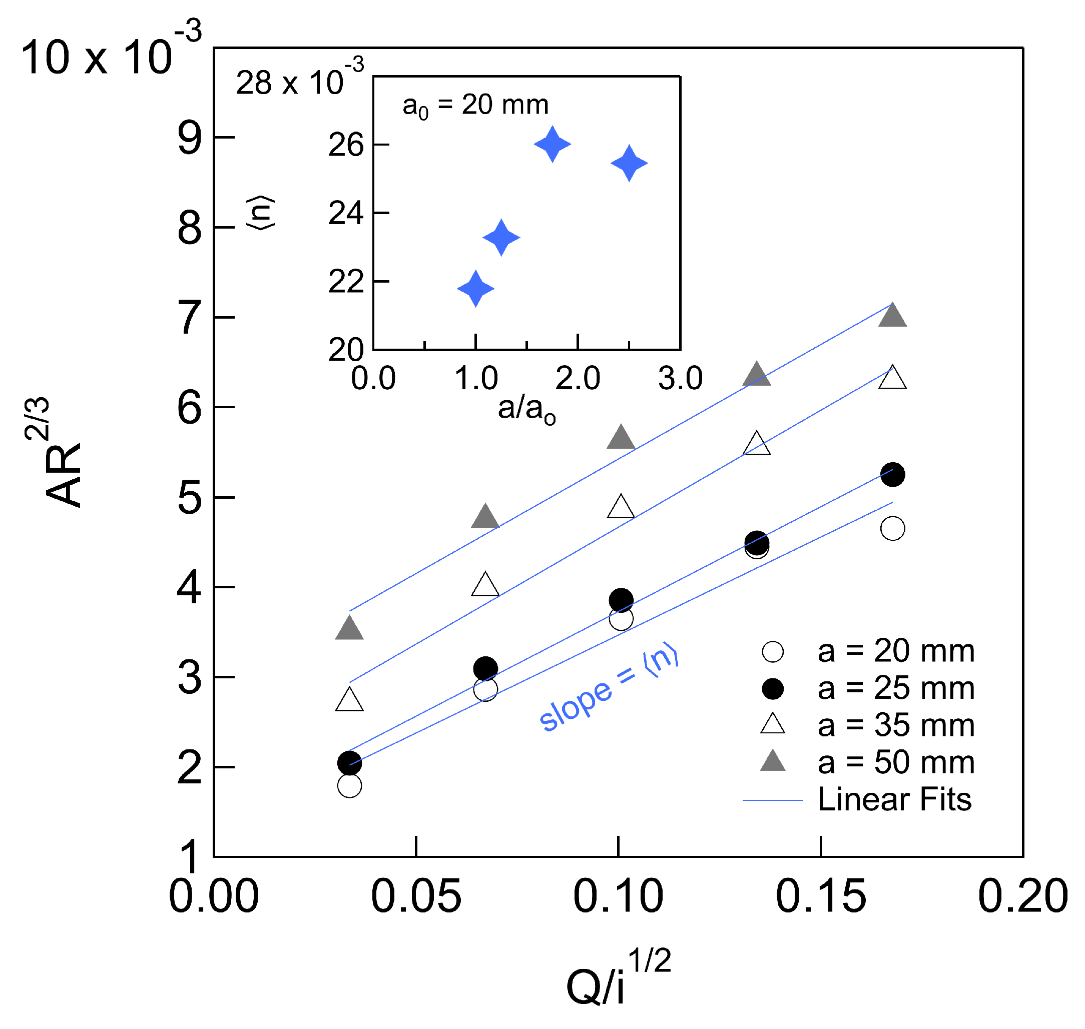
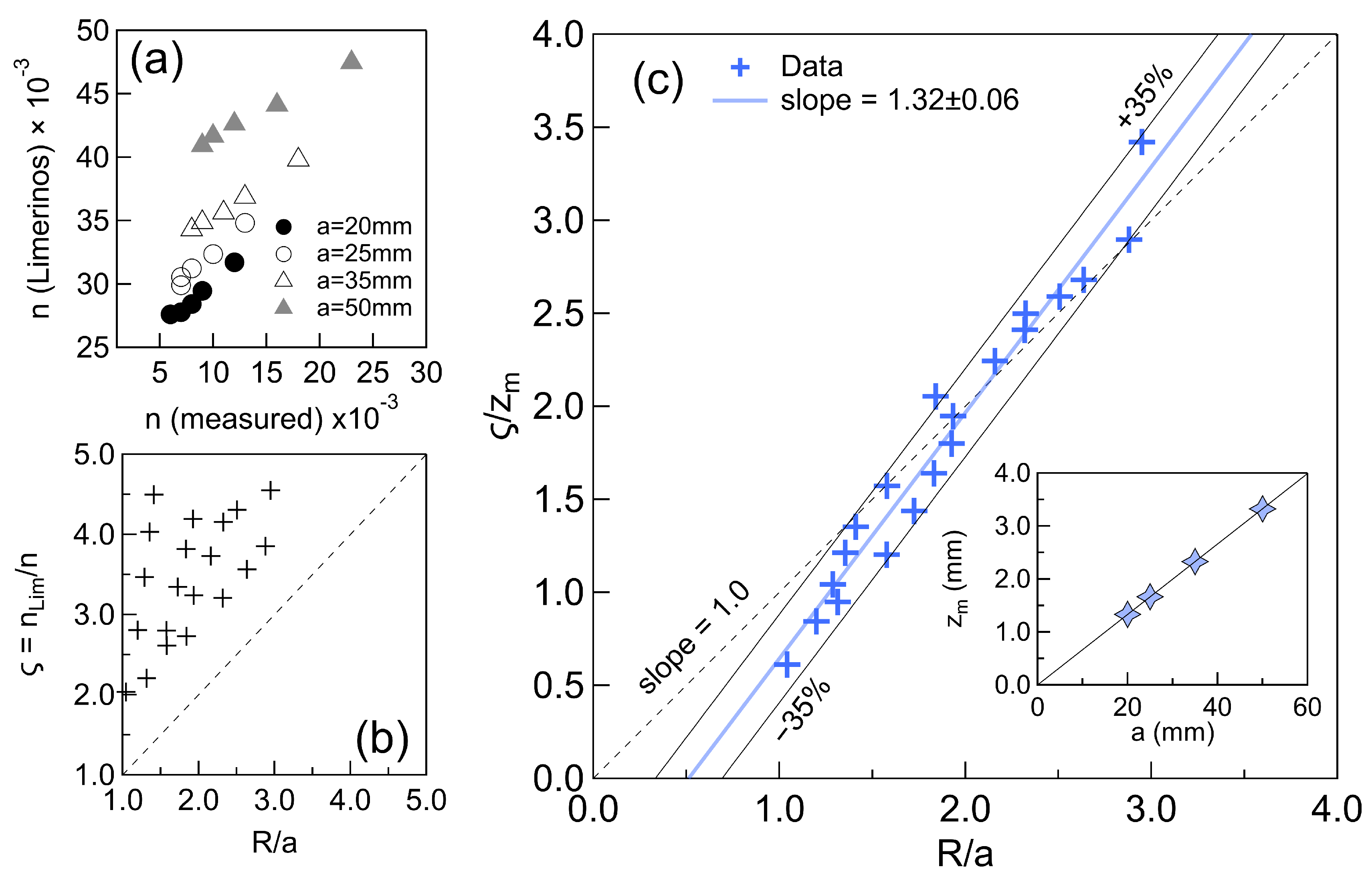
3.5. Determination of the Manning Roughness Coefficient

In addition to the Darcy friction factor, another critical resistance parameter in hydraulic engineering is the Manning roughness coefficient, n [23]. While this parameter has been extensively characterized for a variety of flow conditions and surface types, its behavior in macro-roughness regimes—particularly those involving large, discrete obstacles—remains relatively unexplored. This section evaluates the Manning coefficient under such conditions and investigates its dependence on flow parameters and obstacle geometry.
The Manning law can be written (in SI units) as follows:
Q n J = A R 2 / 3
where Q is the flow rate, J is the friction slope (equal to i for uniform flow), A = W h N is the cross-sectional area, and R is the hydraulic radius. Rearranging Equation (24) under uniform conditions allows for the direct estimation of the Manning coefficient as follows:
n = i Q ( W h N ) W h N W + 2 h N 2 / 3
Figure 11 shows the relationship between Q / i and A R 2 / 3 , revealing highly linear trends for all arrays. This consistency supports the conclusion that the measured normal depth h N satisfies the structural form of Manning’s law. The slope of each line, denoted as n , represents an average roughness coefficient for each configuration. As shown in the inset of Figure 11, n increases with cylinder radius a, except in the case of the largest cylinders (a = 50 mm), for which a decrease is observed. These trends suggest the existence of an empirical function Ψ ( a ) such that n = Ψ ( a ) .
To explore this further, the estimated values of n were compared against those predicted by widely used empirical formulas. One of the most cited formulations is that of Limerinos [45], who developed a correlation for gravel-bed streams based on data from 11 natural rivers in California. Limerinos’ equation is given by the following:
n L i m = 0.0916 κ R 1 / 6 1.16 + 2 log R L
where κ = 1.219 for SI units [46], and L is a representative roughness length scale. Limerinos adopted L = d 84 (the 84th percentile grain size), but in our experiments, the obstacle radius a is a more appropriate choice for L .
Figure 12a compares the Manning coefficients obtained via Equation (26) and those predicted by Limerinos’ formula. The results align along nearly linear trends, but notable discrepancies remain. To further examine these differences, we introduce the ratio ζ = n L i m / n and evaluate it against parameter R / a , as shown in Figure 12b. Although ζ > 1 for all cases, no clear collapse of data is observed.
To better characterize the discrepancy, we define a geometric roughness scale, z m , representing the average vertical projection of the bottom surface over a single spacing interval as follows:
z m = 1 e 0 e z ( x ) d x
where z ( x ) denotes the vertical bed profile and is defined piecewise over the domain x [ 0 , e ] as follows (cf. Figure 13):
z ( x ) = a 2 x 2 , x [ 0 , a ] 0 , x [ a , e a ] a 2 ( x ( e a ) ) 2 , x [ e a , e ]
Figure 12c depicts the normalized discrepancy ζ / z m versus R / a , showing a marked improvement in data collapse, with all points falling within a ± 35 % scatter band. Additionally, the data align well with a linear fit described by the following:
ζ z m = q ^ R a + p ^
where q ^ = 1.32 ± 0.1 and p ^ = 0.68 ± 0.1 are fitting parameters (the units of q ^ are m−1). The inset of Figure 12c confirms the linear relationship between z m and a, described by z m = k · a , with k = 0.067 . Substituting into Equation (26), the relationship simplifies to the following:
n L i m n R
This final result implies that the discrepancy between Limerinos’ formulation and our empirical observations can be attributed to a scaling factor proportional to the hydraulic radius R. It also emphasizes that even for roughness regimes driven by macro-scale geometry, the Manning coefficient remains sensitive to hydraulic geometry and flow structure—particularly the submergence and spatial organization of roughness elements.

4. Conclusions

The study of the friction laws in the macro-roughness regime presents a significant challenge in civil and hydraulic engineering, with implications for both environmental and industrial applications. This research has experimentally investigated the Darcy–Weisbach and Manning roughness coefficients under subcritical, uniform, and turbulent flow conditions over a train of large half-cylindrical roughness elements. The following key conclusions were drawn:
  • The free surface deformation is strongly influenced by the size of the cylinders, producing patterns whose amplitudes correlate with the normal flow depth ( h N ) and the Froude ( F r ) and Reynold numbers ( R e ).
  • The shape of the surface waves closely resembles those reported in previous studies (e.g., [15,34]). However, their amplitudes could not be satisfactorily described using a single empirical function.
  • The Darcy friction factor (f) exhibits a strong inverse relationship with the submergence ratio h N / a , and this trend is similarly observed with R e . These relationships yield robust scaling laws consistent with the early observations of Bazin and Darcy, despite their use of rectangular rather than cylindrical roughness elements.
  • The coefficient f follows a Nikuradse-type logarithmic law, with empirical fitting parameters dependent on cylinder size, spacing, and flow regime (as captured by F r ). The friction factor reaches notably high values, in some instances exceeding 2, reflecting the pronounced energy dissipation in this flow regime.
  • An unexpected yet important finding is that Manning’s resistance law is also recoverable from the experimental data. The Manning coefficient (n) shows a clear dependence on the cylinder radius. A detailed analysis reveals new scaling relationships for n as functions of R / a , reaffirming that submergence ratios—expressed either as R / a or h N / a —play a central role in controlling flow resistance.
Finally, further research is warranted to deepen our understanding of the empirical coefficients derived in this study, particularly in relation to the spacing ratio ξ and the Froude number. The spacing ratio is a critical parameter that may govern transitions between flow regimes, such as skimming and wake-interference flows, which merit comprehensive future investigation.

Author Contributions

Conceptualization, F.M.; methodology, F.M.; formal analysis, F.M.; investigation, F.M. and J.F.; resources, F.M.; data curation, F.M.; writing—original draft preparation, F.M.; writing—review and editing, F.M.; visualization, J.F.; supervision, F.M.; project administration, F.M.; funding acquisition, F.M. All authors have read and agreed to the published version of the manuscript.

Funding

This research was funded by the Vicerrectoría de Investigación of the Pontificia Universidad Católica de Valparaíso through the grants Investigador Emergente (Code 039.329/2022), DI Iniciación (Code 039.326/2023), and Proyecto Puntaje de Corte (Code 210.703/2024).

Data Availability Statement

Experimental data and videos are available upon request to corresponding author.

Acknowledgments

The authors acknowledge the School of Civil Engineering for providing the facilities to conduct this research, and H. Tapia (School of Civil Engineering, PUCV) for their technical support. The authors also thank A. Tamburrino (U. de Chile) for reviewing an earlier version of this manuscript. We are deeply grateful to A. Lopez (School of Civil Engineering, PUCV) for his assistance with the language editing of this manuscript.

Conflicts of Interest

The authors declare that they have no conflicts of interest.

Abbreviations

The following abbreviations are used in this manuscript:
PUCVPontificia Universidad Catolica de Valparaíso

Nomenclature

The following nomenclauture and symbols are used in this manuscript:
ν Fluid kinematic viscosity
ρ Fluid density
δ Boundary layer thickness
u * Shear velocity
UVelocity of the approximating flow
aRadius of the cylinders
h ( x ) Time average of flow depth at a given position x
h N Normal depth of the flow
Δ h Amplitude of the surface waves
RHydraulic depth
QFlow rate
WWidth of the flume
AWetted area
VCross-section average velocity of the flow
F r Froude number
R e Reynolds number
fDarcy’s hydrodynamic friction factor
f C W Colebrook–White friction factor
ε Wall roughness size
nManning roughness coefficient
n L i m Limerinos roughness coefficient
JFriction or energy slope
iBottom slope of the flume

References

  1. Parker, G. 1D Sediment Transport Morphodynamics with Applications to Rivers and Turbidity Currents; CSDMS: Boulder, CO, USA, 2004; Volume 13, p. 2006. [Google Scholar]
  2. Bathurst, J.C. Flow resistance estimation in mountain rivers. J. Hydraul. Eng. 1985, 111, 625–643. [Google Scholar] [CrossRef]
  3. Aguirre-Pe, J.; Fuentes, R. Resistance to flow in steep rough streams. J. Hydraul. Eng. 1990, 116, 1374–1387. [Google Scholar] [CrossRef]
  4. Nicosia, A.; Carollo, F.G.; Ferro, V. Effects of boulder arrangement on flow resistance due to macro-scale bed roughness. Water 2023, 15, 349. [Google Scholar] [CrossRef]
  5. Abulnaga, B. Slurry Systems Handbook; McGraw Hill: New York, NY, USA, 2002. [Google Scholar]
  6. Oke, T.R. Street design and urban canopy layer climate. Energy Build. 1988, 11, 103–113. [Google Scholar] [CrossRef]
  7. Aberle, J.; Smart, G. The influence of roughness structure on flow resistance on steep slopes. J. Hydraul. Res. 2003, 41, 259–269. [Google Scholar] [CrossRef]
  8. Bathurst, J.C. Flow resistance of large-scale roughness. J. Hydraul. Div. 1978, 104, 1587–1603. [Google Scholar] [CrossRef]
  9. Bathurst, J.C.; Simons, D.B.; Li, R.M. Resistance equation for large-scale roughness. J. Hydraul. Div. 1981, 107, 1593–1613. [Google Scholar] [CrossRef]
  10. Cassan, L.; Tien, T.D.; Courret, D.; Laurens, P.; Dartus, D. Hydraulic resistance of emergent macroroughness at large Froude numbers: Design of nature-like fishpasses. J. Hydraul. Eng. 2014, 140, 04014043. [Google Scholar] [CrossRef]
  11. Coleman, S.; Nikora, V.I.; McLean, S.; Schlicke, E. Spatially averaged turbulent flow over square ribs. J. Eng. Mech. 2007, 133, 194–204. [Google Scholar] [CrossRef]
  12. Djenidi, L.; Elavarasan, R.; Antonia, R. The turbulent boundary layer over transverse square cavities. J. Fluid Mech. 1999, 395, 271–294. [Google Scholar] [CrossRef]
  13. Hey, R.D. Flow resistance in gravel-bed rivers. J. Hydraul. Div. 1979, 105, 365–379. [Google Scholar] [CrossRef]
  14. Thappeta, S.K.; Bhallamudi, S.M.; Fiener, P.; Narasimhan, B. Resistance in steep open channels due to randomly distributed macroroughness elements at large Froude numbers. J. Hydrol. Eng. 2017, 22, 04017052. [Google Scholar] [CrossRef]
  15. Stoesser, T.; Nikora, V.I. Flow structure over square bars at intermediate submergence: Large Eddy Simulation study of bar spacing effect. Acta Geophys. 2008, 56, 876–893. [Google Scholar] [CrossRef]
  16. Colosimo, C.; Copertino, V.A.; Veltri, M. Friction factor evaluation in gravel-bed rivers. J. Hydraul. Eng. 1988, 114, 861–876. [Google Scholar] [CrossRef]
  17. Ferguson, R. Flow resistance equations for gravel-and boulder-bed streams. Water Resour. Res. 2007, 43, 1–12. [Google Scholar] [CrossRef]
  18. Kumar, B. Flow resistance in alluvial channel. Water Resour. 2011, 38, 745–754. [Google Scholar] [CrossRef]
  19. Pagliara, S.; Chiavaccini, P. Flow resistance of rock chutes with protruding boulders. J. Hydraul. Eng. 2006, 132, 545–552. [Google Scholar] [CrossRef]
  20. Pagliara, S.; Das, R.; Carnacina, I. Flow resistance in large-scale roughness condition. Can. J. Civ. Eng. 2008, 35, 1285–1293. [Google Scholar] [CrossRef]
  21. Darcy, H. Recherches Hydrauliques Entreprises par M. Henry Darcy Continuées par M. Henri Bazin. Rapport fait à l’Académie des Sciences sur un Mémoire de M. Bazin sur le Mouvement de l’eau dans les Canaux déCouverts; Imprenta Impériale de París, Dunod: Paris, France, 1865; Volume 1. [Google Scholar]
  22. Perry, A.E.; Schofield, W.H.; Joubert, P.N. Rough wall turbulent boundary layers. J. Fluid Mech. 1969, 37, 383–413. [Google Scholar] [CrossRef]
  23. Chow, V.T. Open-Channel Hydraulics; MC Graw Hill: Seattle, WA, USA, 1988. [Google Scholar]
  24. Lim, H.S. Open channel flow friction factor: Logarithmic law. J. Coast. Res. 2018, 34, 229–237. [Google Scholar] [CrossRef]
  25. Davis, J.; Barmuta, L. An ecologically useful classification of mean and near-bed flows in streams and rivers. Freshw. Biol. 1989, 21, 271–282. [Google Scholar] [CrossRef]
  26. Morris, H.M., Jr. Flow in rough conduits. Trans. Am. Soc. Civ. Eng. 1955, 120, 373–398. [Google Scholar] [CrossRef]
  27. Morris, H.N. A new concept of flow in rough conduits. In Proceedings of the American Society of Civil Engineers; ASCE: Reston, VA, USA, 1955; Volume 80, pp. 1–31. [Google Scholar]
  28. Oke, T.R. Boundary Layer Climates; Routledge: London, UK, 2002. [Google Scholar]
  29. Nikora, V.; McEwan, I.; McLean, S.; Coleman, S.; Pokrajac, D.; Walters, R. Double-averaging concept for rough-bed open-channel and overland flows: Theoretical background. J. Hydraul. Eng. 2007, 133, 873–883. [Google Scholar] [CrossRef]
  30. Lawrence, D. Macroscale surface roughness and frictional resistance in overland flow. Earth Surf. Process. Landforms J. Br. Geomorphol. Group 1997, 22, 365–382. [Google Scholar] [CrossRef]
  31. Lawrence, D. Hydraulic resistance in overland flow during partial and marginal surface inundation: Experimental observations and modeling. Water Resour. Res. 2000, 36, 2381–2393. [Google Scholar] [CrossRef]
  32. Nikuradse, J. Laws of Flow in Rough Pipes; NACA TN 1292; NASA: Washington, DC, USA, 1950.
  33. Bayazit, M. Free surface flow in a channel of large relative roughness. J. Hydraul. Res. 1976, 14, 115–126. [Google Scholar] [CrossRef]
  34. McSherry, R.; Chua, K.; Stoesser, T.; Mulahasan, S. Free surface flow over square bars at intermediate relative submergence. J. Hydraul. Res. 2018, 56, 825–843. [Google Scholar] [CrossRef]
  35. Schindler, R.J.; Ackerman, J.D. The environmental hydraulics of turbulent boundary layers. In Advances in Environmental Fluid Mechanics; World Scientific: Singapore, 2010; pp. 87–125. [Google Scholar]
  36. Martinez, F.; Farias, J. Friction factor and surface deformation of subcritical flows on a train of cylindrical ribs. In Proceedings of the 12th International Conference on Fluvial Hydraulics, River Flow, Liverpool, UK, 2–6 September 2024; CRC Press: Boca Raton, FL, USA, 2025; pp. 359–367. [Google Scholar]
  37. Forbes, L.K.; Schwartz, L.W. Free-surface flow over a semicircular obstruction. J. Fluid Mech. 1982, 114, 299–314. [Google Scholar] [CrossRef]
  38. Vigié, F. Etude Expérimentale d’un écoulement à surface Libre Au-Dessus d’un Obstacle. Ph.D. Thesis, Institut National Polytechnique, Toulouse, France, 2005. [Google Scholar]
  39. Ryu, D.; Choi, D.H.; Patel, V. Analysis of turbulent flow in channels roughened by two-dimensional ribs and three-dimensional blocks. Part I: Resistance. Int. J. Heat Fluid Flow 2007, 28, 1098–1111. [Google Scholar] [CrossRef]
  40. Monin, A.; Yaglom, A. Statistical Fluid Mechanics: Mechanics of Turbulence; MIT Press: Cambridge, MA, USA, 1975; Volume 1, 874p. [Google Scholar]
  41. Pokrajac, D.; Campbell, L.J.; Nikora, V.; Manes, C.; McEwan, I. Quadrant analysis of persistent spatial velocity perturbations over square-bar roughness. Exp. Fluids 2007, 42, 413–423. [Google Scholar] [CrossRef]
  42. Choo, Y.M.; Kim, J.G.; Park, S.H. A Study on the friction factor and Reynolds number relationship for flow in smooth and rough channels. Water 2021, 13, 1714. [Google Scholar] [CrossRef]
  43. Blasius, H. Das aehnlichkeitsgesetz bei reibungsvorgängen in flüssigkeiten. In Mitteilungen über Forschungsarbeiten auf dem Gebiete des Ingenieurwesens: Insbesondere aus den Laboratorien der Technischen Hochschulen; Springer: Berlin/Heidelberg, Germany, 1913; pp. 1–41. [Google Scholar]
  44. Colebrook, C.F. Turbulent flow in pipes, with particular reference to the transition region between the smooth and rough pipe laws. Journal of the Institution of Civil Engineers 1939, 11, 133–156. [Google Scholar] [CrossRef]
  45. Limerinos, J.T. Determination of the Manning Coefficient from Measured Bed Roughness in Natural Channels; US Government Printing Office: Washington, DC, USA, 1970.
  46. HEC-RAS 2D Sediment Technical Reference Manual. Available online: https://www.hec.usace.army.mil/confluence/rasdocs/d2sd/ras2dsedtr/latest/model-description/bedform-geometry-and-hydraulic-roughness/bottom-roughness (accessed on 21 March 2024).
Figure 1. Different roughness regimes in open channel flows. (a) Isolated regime, (b) wake interference, and (c) quasi-smooth flow (adapted from Oke [28]).
Water 17 01301 g001
Figure 2. Schematic view of the experimental setup and its components. (a) Schematic view of the flume and its components; (b) a view of the cylinders used to build the arrays; (c) shows the positions of the ultrasound probes used for the depth measurements and (d), an overall view of the free surface deformation when interacting with the cylinders.
Water 17 01301 g002
Figure 3. Flow’s free surface deformation for increasing flow rates, with cylinders of radius a = 25 mm. (a) Q = 3.0 Ls−1, (b) Q = 6.0 Ls−1, and (c) Q = 15.0 Ls−1. Distinct deformation patterns can be observed across the experiments. As expected, as Q increases, the normal height h N also increases. Valleys and peaks of each profile are also shown.
Water 17 01301 g003
Figure 4. Free surface flow deformation for Q = 15 Ls−1 and increasing cylinder sizes: (a) a = 20 mm, (b) a = 35 mm, and (c) a = 50 mm.
Water 17 01301 g004
Figure 5. Evolution of the surface waves observed for the experiment with Q = 15 Ls−1 and a = 25 mm. The sequence captures one full cycle with a duration of approximately Δ T 1 s. The red arrow indicates the position of a wave peak, from its maximum amplitude to its disappearance, with the cycle repeating after each Δ T .
Water 17 01301 g005
Figure 6. Backwater profiles obtained for Q = 3 , 6 , 12 Ls−1, and radius (a) a = 20 mm, (b) a = 25 mm, (c) a = 35 mm, and (d) a = 50 mm. In (a) the normal depth h N and the amplitude Δ h = h m a x h m i n were included, where h m i n , h m a x is the streamwise average of the valleys and peaks of each profile, respectively.
Water 17 01301 g006
Figure 7. Relative average deformation of the free surface, Δ h / a , plotted against: (a) h N / a , (b) F r , and (c) R e for different arrays of cylinders.
Water 17 01301 g007
Figure 8. (a) Relative depth h N / a vs. h / a for all the experiments. The inset shows a comparison between flow depth h N and h N 0 for the same dataset. (b) h N vs. the streamwise Froude number F r (as defined in Equation (10)), for all the arrays. (c,d) Parameters m * and n * plotted against cylinder radius a.
Water 17 01301 g008
Figure 9. (a) h N / a vs. F r for different cylinders radii. The fitting curve corresponds to Equation (14). (b) h N / a versus R e / R e c , with the fitting lines given by Equation (15), having slope d. (c,d) Parameters c and d versus a / a o , where a o = 20 mm. The decreasing fitting lines are defined by Equations (16) and (17).
Water 17 01301 g009
Figure 11. Distribution of the Manning’s roughness coefficient based on Equation (24). From the fitting lines to the curves of A R 2 / 3 vs. Q / i , an average roughness coefficient n was obtained as the slope for each array. The inset shows n vs. a / a o .
Water 17 01301 g011
Figure 12. Scaling law for the Manning roughness coefficient. (a) Comparison n L i m and n for all the experimental runs. (b) Ratio ζ = n L i m / n vs. R / a . (c) ζ / z m vs. R / a , with the central fitting line given by Equation (29). All the points fall within a ± 35 % scattering band. A unit-slope line is included as a visual guide. The inset shows the parameter z m vs. a, with the slope of the fitting line given by k = 0.067 .
Water 17 01301 g012
Figure 13. Scheme adopted for the definition of the parameter z m .
Water 17 01301 g013
Table 1. Experimental arrays used in the study. Here, a denotes the radius of the cylinders, e the spacing between them and N the total number of obstacles. The variation range of the normal depth h N was also included.
Arraya
(mm)
e
(mm)
N
-
h N
(mm)
120.0255.33946.4–88.1
225.0319.13150.6–95.9
335.0446.72261.1–108.9
450.0638.21672.6–117.3
Disclaimer/Publisher’s Note: The statements, opinions and data contained in all publications are solely those of the individual author(s) and contributor(s) and not of MDPI and/or the editor(s). MDPI and/or the editor(s) disclaim responsibility for any injury to people or property resulting from any ideas, methods, instructions or products referred to in the content.

