Article

Improved Resolution of Drought Monitoring in the Yellow River Basin Based on a Daily Drought Index Using GRACE Data

1
School of Surveying and Land Information Engineering, Henan Polytechnic University, Jiaozuo 454003, China
2
School of Information Science and Engineering, Harbin Institute of Technology, Weihai 264209, China
3
School of Geomatics, Liaoning Technical University, Fuxin 123000, China
4
Satellite Application Center for Ecology and Environment, Ministry of Ecology and Environment, Beijing 100094, China
*
Authors to whom correspondence should be addressed.
Water 2025, 17(9), 1245; https://doi.org/10.3390/w17091245
Submission received: 19 March 2025 / Revised: 15 April 2025 / Accepted: 19 April 2025 / Published: 22 April 2025

Abstract

:
Frequent droughts significantly threaten economic development, necessitating effective long-term drought monitoring. The Gravity Recovery and Climate Experiment (GRACE) satellite and its follow-on mission along with Global Navigation Satellite System (GNSS) inversion technologies provide long-term terrestrial water storage signals. However, their limitations in temporal resolution and spatial continuity are inadequate for current requirements. To solve this problem, this study combines a daily terrestrial water storage anomaly (TWSA) reconstruction method with the GNSS inversion technique to explore daily, spatially continuous TWSA in China’s Yellow River Basin (YRB). Furthermore, the Daily Drought Severity Index (DDSI) is employed to analyze drought dynamics in the YRB. Finally, by reconstructing the climate-driven water storage anomalies model, this study explores the influence of climate and human factors on drought. The results indicate the following: (1) The reconstructed daily TWSA product demonstrates superior quality compared to other available products and exhibits a discernible correlation with GNSS-derived daily TWSA data, while REC_TWSA is closer to the GRACE-based TWSA dataset. (2) The DDSI demonstrates superior drought monitoring capabilities compared to conventional drought indices. During the observation period from 2004 to 2021, the DDSI detected the most severe drought event occurring between 30 October 2010 and 10 September 2011. (3) Human activities become the primary driver of drought in the YRB. The high correlation of 0.81 between human-driven water storage anomalies and groundwater storage anomalies suggests that the depletion of TWSA is due to excessive groundwater extraction by humans. This study aims to provide novel evidence and methodologies for understanding drought dynamics and quantifying human factors in the YRB.

1. Introduction

Climate change is a global challenge facing the world at present, and its impacts are becoming more visible [1]. In recent years, disasters triggered by extreme climate change have been occurring frequently, and hydro-geological calamities such as floods and droughts have received widespread attention [2]. In particular, as a broadly spread and frequent disaster, drought not only hinders social and economic development, but also raises a series of environmental issues, such as land degradation, dust storms, and desertification [3,4].
Since its launch in 2002, the Gravity Recovery and Climate Experiment (GRACE) satellite and its follow-on mission (GRACE-FO) have provided global monthly terrestrial water storage anomaly (TWSA) data by monitoring changes in the Earth’s gravity field [5]. GRACE opens a new approach to monitoring extreme hydrological events with its comprehensive spatial coverage, high accuracy, and independence from weather conditions [6]. The reliability of GRACE TWSA has been demonstrated by scholars at home [7,8,9,10] and abroad [11,12] by assessing it with hydrological modeling data. GRACE has also been used to invert the spatial and temporal variations in groundwater storage, which displays a significant correlation with in-situ groundwater level data [13,14].
Actually, GRACE has a high degree of precision. However, GRACE is also limited by its coarse temporal and spatial resolution as well as missing time series, which restrict its application in hydrological studies greatly. Its spatial and temporal resolution has been improved recently and achieved remarkable progress [15,16]. In spatial downscaling, most methods are used to enhance the original resolution of GRACE such as machine learning and random forests [17,18,19]. For temporal downscaling, daily GRACE gravity field solutions are used to evaluate the major flood events based on the Kalman filter method [20]. Nevertheless, the publicly released ITSG-GRACE 2018 daily data has a time delay of several months [21], which is not sufficient for accurate monitoring of flooding events. Humphrey and Gudmundsson [22] have reconstructed the daily TWSA with a spatial resolution of 0.5° using a statistical model, which is trained on the GRACE data in combination with the meteorological dataset. Humphrey’s method is used to reconstruct the daily TWSA for northern Henan Province and the wetness index is employed for flood warnings [23]. Wang et al. [24] similarly utilized Humphrey’s reconstruction method to obtain daily TWSA of the Pearl River Basin and calculate a daily drought severity index (DSI) based on these data that accurately detects drought conditions. It is demonstrated that the reconstructed daily TWSA are more likely to be used for flood and drought monitoring in the watershed than other daily TWSA.
With the advancement of Global Navigation Satellite System (GNSS) technology, it has been proven to be effective in monitoring displacements caused by changes in surface mass loading [25]. Particularly in regions with significant water storage variations, the periodic changes in the GNSS time series exhibit a high level of consistency with the GRACE-derived hydrologic load deformation displacements [26,27]. The crustal displacement changes obtained from GNSS can be used to further invert the regional TWSA quantitatively [28,29]. For instance, Jiang et al. [30] recovered daily variations in water storage in China based on the spherical Slepian basis function. Peng et al. [31] investigated the extreme hydrological drought in the Poyang Lake Basin using the daily GNSS-DSI, which proves to be more sensitive to drought signals on a local time scale.
The exacerbation of drought in China’s Yellow River Basin (YRB) has led to reduced crop yields, river drying, and tensions in residential and industrial water usage, highlighting the urgency and importance of in-depth research into drought characteristics. Studies on drought in the YRB mostly involve monitoring and analysis of different drought indices at monthly scales. For instance, the monthly and annual Palmer drought severity index (PDSI) is used to identify the increasing frequency of extreme droughts in the YRB [32]; the joint drought index (JDI) is constructed using the Gaussian Copula function and combining the standardized precipitation index (SPI) on multiple time scales. It is found that the JDI has a greater advantage in capturing drought propagation and evolution compared to the SPI [33]; the water storage deficit index (WSDI) is compared and analyzed with other drought indices, such as standardized precipitation evapotranspiration index (SPEI), to confirm the validity of the WSDI in the identification of large-scale drought events [34]. However, the above studies do not meet the needs for practical applications, which makes it difficult to assess the evolution of the spatial details of drought events.
Compared to previous studies, we construct the Daily Drought Severity Index (DDSI) by reconstructing the daily TWSA to monitor the spatial and temporal evolution of drought in the YRB. Moreover, we analyze the drought-influencing factors using climate-driven water storage anomalies (CWSA) reconstruction models. The main objectives of this work are (1) to reconstruct the daily TWSA and evaluate the reconstructed data in this paper with GNSS and other data; (2) to calculate the DDSI, evaluate it in different drought indices, and analyze the spatial and temporal evolution of drought in the YRB based on the DDSI; and (3) to separate the CWSA and HWSA and to analyze the factors affecting drought in the YRB.

2. Study Area and Datasets

2.1. Study Area

The Yellow River is the second longest river in China, with a length of over 5464 km. The YRB covers about 795,000 km2 and ranges from 96° E to 119° E and 32° N to 42° N on Earth. This region gradually decreases in elevation from west to east. The west is mainly dominated by high mountains, while the eastern region suffers from flooding [35,36]. Located in the mid-latitudes, the YRB relies on natural precipitation to recharge the water reserves. However, the rainfall in the region is low and spatially uneven [37]. In addition, the utilization rate of water resources is as high as 80%, exceeding the ecological red line of 40% [38], which seriously hampers the sustainable development of the basin. Based on hydrological and geographic features, the whole basin is usually divided into three regions: the upper, the middle, and the lower reaches (Figure 1).

2.2. Data

2.2.1. TWSA Products

Monthly TWSA derived from the GRACE/GRACE-FO RL06 Mascon solution (version 02) are used in this study, and these Mascon data are from the Jet Propulsion Laboratory (JPL) and the Center for Space Research (CSR) at the University of Texas at Austin, respectively. Compared to the previous version, RL06 Mascon has less data noise and relieves the quality leakage problem while preserving the important signals [39,40]. In this study, TWSA data are provided by CSR and JPL with actual spatial resolutions of 1° and 3°, respectively, but with products released at 0.25° and 0.5°. These datasets are referred to as CSR_TWSA and JPL_TWSA, respectively.
Daily TWSA products are provided by several organizations. Specifically, the Global Land Data Assimilation System (GLDAS) includes four land-surface models, catchment land surface model (CLSM), Mosaic, NOAH, and VIC. Daily TWSA data are used in this study with a spatial resolution of 0.25° from GLDAS-CLSM v2.2, and this dataset is referred to as GLDAS_TWSA [41,42]. The ITSG-Grace 2018 gravity field model provides daily TWSA, realized by adding Kalman smoothed daily solutions to the original model [21,43]. The daily TWSA datasets JPL_ERA5 and JPL_MSWEP are reconstructed by Humphrey and Gudmundsson [22] using JPL_TWSA, ERA5 precipitation, and Multi-Source Weighted Ensemble Precipitation (MSWEP) data, both with 0.5° spatial resolution.

2.2.2. Temperature and Precipitation Data

Two types of precipitation and temperature data are used to construct the reconstruction models: CN05.1 and ERA5. Specifically, CN05.1 is based on data from over two thousand weather stations in China and utilizes interpolation to generate meteorological data with a spatial resolution of 0.25°, including daily precipitation and temperature [44,45,46]. Nie et al. [47] suggest that using the CN05.1 dataset to reconstruct daily TWSA is better than others. Thus, the CN05.1 data are used to reconstruct the daily TWSA directly. ERA5 is the fifth generation of reanalysis data that is provided by the European Center for Medium-Range Weather Forecasts (ECMWF), and ERA5-Land is an enhanced global dataset for the land component of ERA5 [48]. The ERA5 provides a strong level of consistency with the in-situ data with high confidence [49,50]. In this study, the monthly precipitation and temperature data provided by ERA5-Land are used to reconstruct CWSA.

2.2.3. GNSS Data

The time series data of GNSS stations are obtained from the China Earthquake Science Data Center (CEDC, https://www.eqdsc.com accessed on 24 March 2024) and are calculated using the GAMIT/GLOBK 10.40 and QOCA software developed by the Massachusetts Institute of Technology. Non-tidal atmospheric loading (NTAL) and non-tidal oceanic loading (NTOL) are released by the Earth System Modeling group at Deutsches GeoForschungsZentrum (ESMGFZ, http://esmdata.gfz-potsdam.de:8080/repository accessed on 14 May 2024), and these are utilized to correct for their effects on the GNSS vertical coordinate time series. The data are averaged to a daily scale as the NTAL and NTOL have a temporal resolution of 3 h.

2.2.4. Drought Index

Wells et al. [51] proposed the self-calibrating Palmer Drought Severity Index (scPDSI), which compensates for the weakness of the traditional PDSI in terms of regional comparability. The scPDSI data are reconstructed to compare the relative availability of moisture in different regions [52]. This study uses the scPDSI dataset published by the Climate Research Center in a monthly 0.5° grid format. According to the existing studies [53], scPDSI is classified into four degrees, as shown in Table 1.
The Standardized Precipitation Index (SPI) and Standardized Precipitation Evapotranspiration Index (SPEI) are the most frequently used drought indices, and the traditional SPI and SPEI are based on monthly time resolution. Wang et al. [54,55] improved the calculation methods of SPI and SPEI and provided a new multi-scale daily SPI and SPEI dataset for China. However, these datasets are released in the form of stations instead of providing rasterized data. Liu et al. [56] developed a global daily SPEI dataset (SPEI-GD) based on the precipitation data of ERA5 and the potential evapotranspiration data of Singer’s dataset, which includes multiple timescales with a spatial resolution of 0.25°.

2.2.5. Auxiliary Datasets
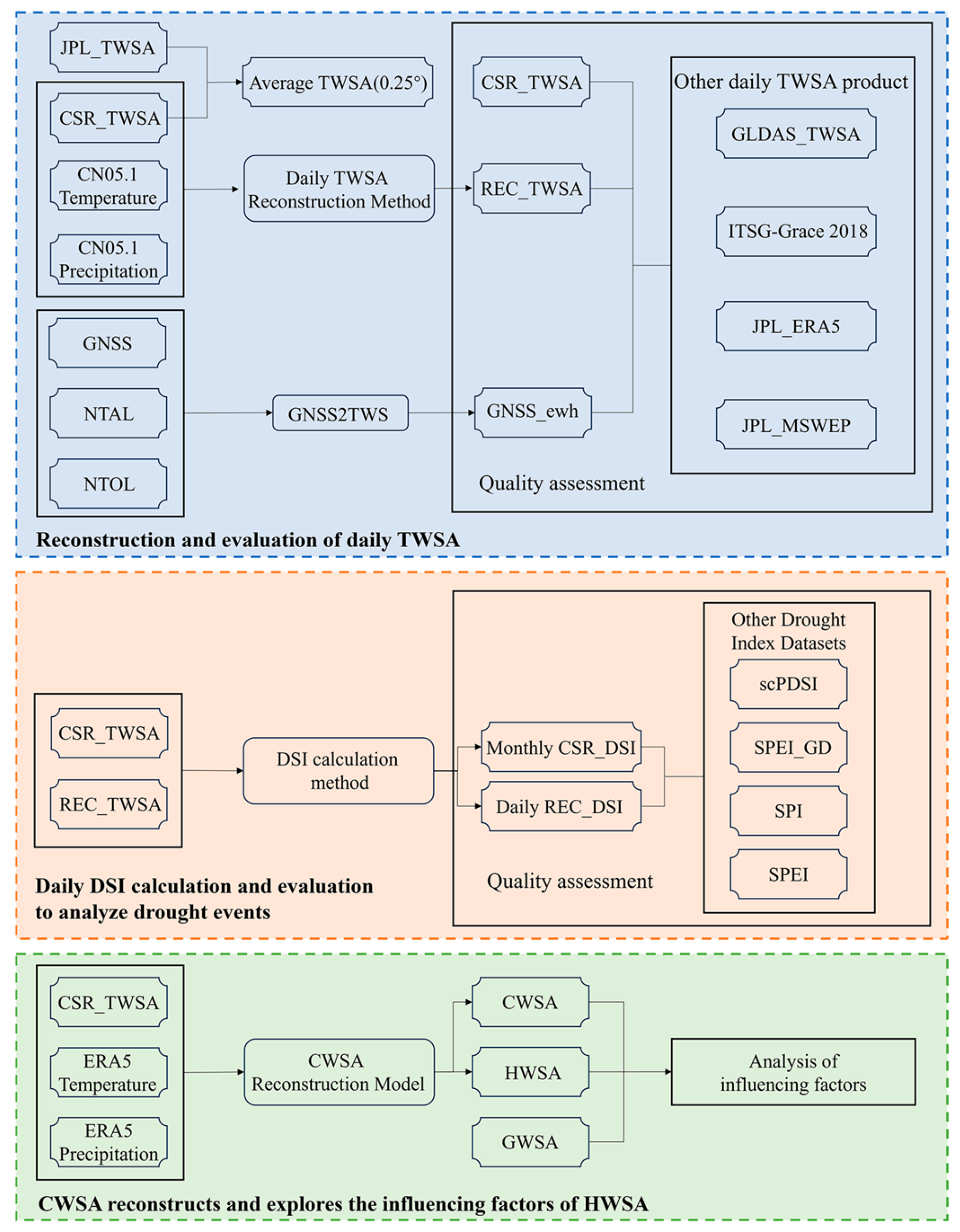
The NOAH land surface model from the GLDAS model provides monthly surface water storage data (0–200 cm soil moisture, snow water equivalent, canopy water evaporation) with a spatial resolution of 0.25° [57,58]. To be consistent with the GRACE data, the average surface water storage from January 2004 to December 2009 is taken as the baseline, and the monthly surface water storage anomalies are obtained after removing the baseline.

3. Method

In this study, two methods are used to obtain daily TWSA data with continuous and high-temporal resolution. On one hand, near real-time precipitation and temperature are used as the driving data to reconstruct high-precision daily TWSA data based on a statistical method combined with time series decomposition. On the other hand, the hydrological load deformation data from GNSS and the open-source tool, GNSS2TWS, are used to derive the daily TWSA data. Then, the quality of the two daily TWSA is assessed using daily TWSA datasets such as GLDAS_TWSA. Secondly, an innovative DDSI is constructed based on the reconstructed TWSA (REC_TWSA), and it is assessed and compared with other drought index datasets to explore the spatial and temporal evolution of drought in the YRB. Finally, the effects of climate and human factors on TWSA are separated based on the CWSA model (Figure 2).

3.1. Daily TWSA Reconstruction Method

Humphrey and Gudmundsson [22] proposed a method to reconstruct the daily and monthly TWSA, and Wang et al. [24] improved it in terms of long-term linear trends. This method is driven by near real-time precipitation and temperature, with GRACE TWSA serving as constraint data. It is capable of reconstructing TWSA data on a daily scale:
T W S A ( t ) = T W S A ( t 1 ) e 1 τ ( t ) + P ( t )
τ ( t ) = a + b T Z ( t )
where t is the daily time series, and T W S A ( t ) , P ( t ) , and T Z ( t ) represent the TWSA, precipitation, and temperature changes at time t, respectively. e 1 / τ ( t ) is solely dependent on temperature. The daily TWSA data obtained through the above method need to be averaged to monthly values. Subsequently, the GRACE TWSA data are constrained using the following equation:
anom ( GRACE ( t m ) ) = β a n o m ( T W S A ( t m ) ) + ε
where β represents the calibration factor, and ε denotes the error. a n o m ( ) represents the removal of linear trend and seasonal components, and the parameters a, b, and β are calibrated using the Markov Chain Monte Carlo (MCMC) method. The missing months of GRACE data are not involved in the parameter adjustments [24]. Daily TWSA that exclude seasonal components and trend components can be obtained using the above formula.

3.2. Time Series Decomposition Method

The daily TWSA data derived in Section 3.1 require the restoration of their trend and seasonal components. In time series analysis, the separation of seasonal and trend components using least squares regression represents a classical signal decomposition methodology. Specifically, the TWSA time series is considered the sum of the long-term trend signal, annual signal, semi-annual signal, and a residual term [59]. It can be calculated using the following mathematical formula:
f ( t ) = a + b ( t t 0 ) + c c o s ( 2 π t ) + d s i n ( 2 π t ) + e c o s ( 4 π t ) + f s i n ( 4 π t ) + ε
where a is the constant term; b is the trend term; c, d, e, and f represent the seasonal terms; and ε indicates the residual term. The parameters are obtained by fitting this function using the least squares method. It is critical to note that the trend and annual cycle components derived from GRACE TWSA decomposition are interpolated to daily equivalents using the least squares method, which is then combined with model-simulated semi-annual cycle components to reconstruct the complete daily TWSA signal.

3.3. GNSS Inversion

Due to the sensitivity of vertical displacement to hydrological mass changes [60,61], only vertical displacement is utilized for inversion modeling. After eliminating influences such as long-term linear trend, NTAL, NTOL, and postseismic deformation, the GNSS vertical time series dominated by hydrological signals is obtained finally. The open-source tool GNSS2TWS [62] is utilized to infer daily TWSA. This software employs principal component analysis combined with spatial domain Green’s function method to invert regional TWSA, enabling the time-varying inversion of vertical displacement time series in dense GNSS networks. Please refer to the citations for detailed data processing and inversion methods [30,62,63]. The methods are described simply as follows:
u = G x
where u is the vertical displacement of GNSS, x represents the gridded mass load, and G is the calculated Green’s function matrix [64]. When solving undetermined parameters, ill-posed problems are often encountered, and regularization techniques are used to minimize the following terms [65,66]:
G x u 2 + α 2 L x 2 = min
where L is the Laplacian smoothing matrix, and α is the smoothing factor. The final result can be determined using the following formula:
x = ( G T G + α 2 L T L ) 1 G T u
To strengthen the comparative validation framework, the daily TWSA derived from the aforementioned GNSS inversion will be employed to verify the accuracy of the prior GRACE-based reconstruction.

3.4. Daily Drought Severity Index

Traditional studies have mostly relied on GRACE to construct a monthly DSI [67,68], but its ability to monitor the temporal evolution of drought is relatively coarse. Building on the framework established by Zhao et al. [69], Wang et al. [24] developed a daily drought severity index to characterize daily drought dynamics in the Pearl River Basin. This study follows the method of Wang et al., employing reconstructed daily TWSA-based GRACE to calculate the DDSI, which quantifies drought severity at a daily temporal resolution. The formula is as follows:
D D S I i , j = T W S A i , j T W S A j ¯ σ j
where i denotes the i-th year. In this study, j represents the j-th day of the year. T W S A j represents the set of TWSA on the same day across different years, while T W S A j ¯ and σ j denote the mean and standard deviation of set T W S A j , respectively.
Drought is categorized into five categories, D0 to D4, based on the recommendations given by the U.S. Drought Detection Agency (Table 1) [69]. Drought is considered to occur when the DSI is less than or equal to −0.5, with lower DSI values indicating more severe drought conditions. Typically, a drought event is declared when the DSI remains less than or equal to −0.5 for a continuous period of three months (90 days) or more.
Characteristics of a drought event mainly include drought duration, drought severity, drought intensity, and the date corresponding to the minimum value of the drought index. Drought duration represents its time span; drought severity indicates the integral of the DSI when it is below a threshold [70]; and drought intensity refers to the minimum value of the drought index within its time range. By calculating DDSI in this study, drought events can be precisely identified at a daily resolution, thus providing more accurate drought onset and cessation dates.

3.5. Reconstruction of Climate-Driven Water Storage Anomalies

CWSA can be reconstructed by precipitation and temperature [22]. Liu et al. [71] propose a new method to reconstruct CWSA based on the water balance equation, using temperature and precipitation as the driving data. This can be represented using the following formula:
H t i + 1 R E C + d = ( H t i R E C + d ) e τ t i + 1 + P t i + 1
τ t i = a + b P t i + c T t i
where t i represents time, and H t i R E C denotes the reconstructed CWSA data at time t i . d represents the active water storage, which is the portion of water involved in the hydrological cycle. P t i represents the precipitation at time t i , and T t i represents the temperature at time t i . P t i and T t i are the normalized precipitation and temperature, respectively. Parameters a, b, c, and d are estimated using the Markov Chain Monte Carlo (MCMC) algorithm.
The total TWSA data are influenced by both climate change and human activities. The CWSA data simulated by this model are derived from precipitation and temperature, excluding anthropogenic factors. Therefore, the human-driven water storage anomalies (HWSA) data can be separated from TWSA and CWSA data with the following calculation formula:
H W S A i s o l a t i o n = T W S A C W S A r e c o n s t r u c t i o n
where H W S A i s o l a t i o n represents the HWSA, and TWSA denotes the TWSA monitored by GRACE.

4. Result

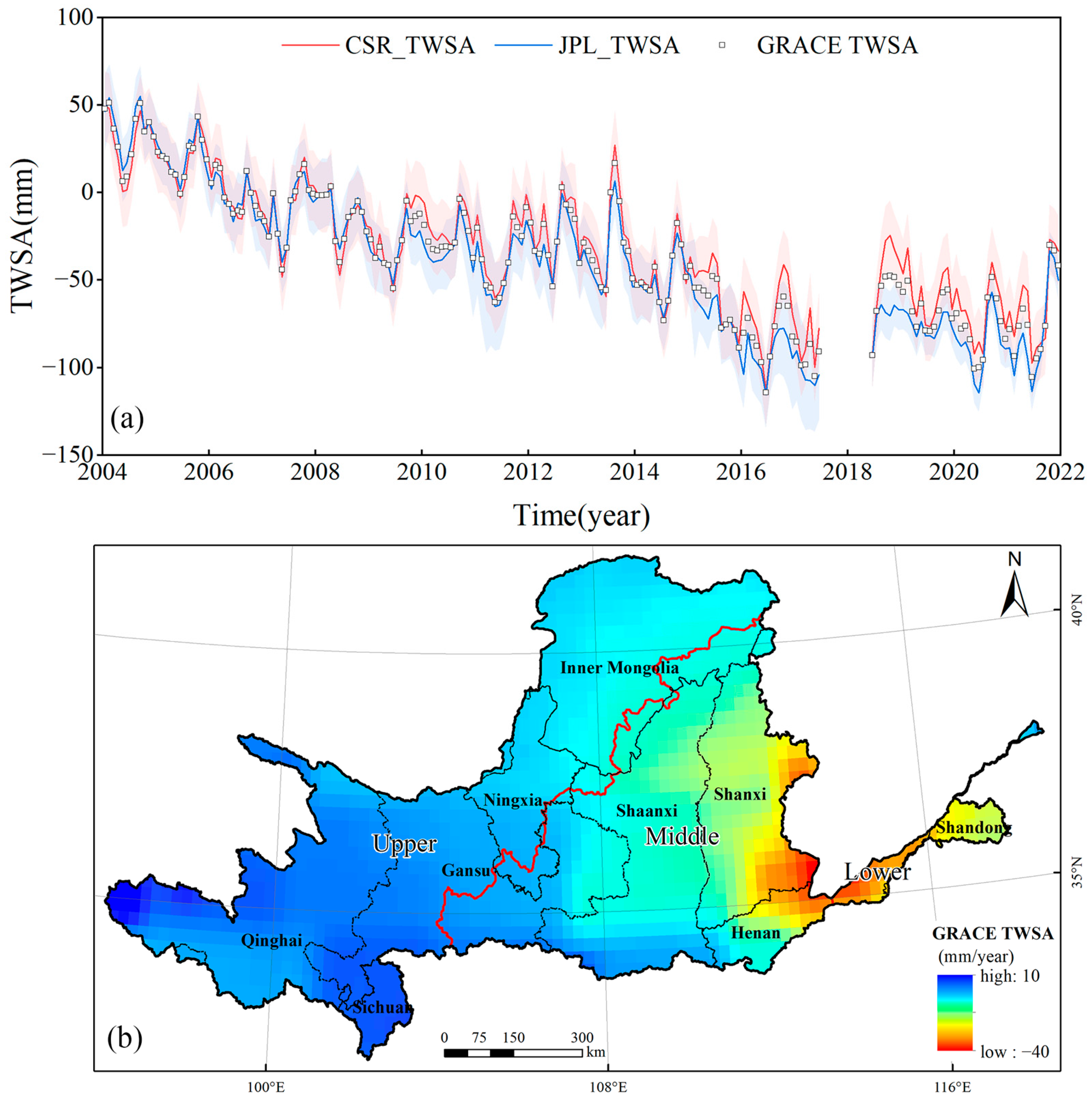
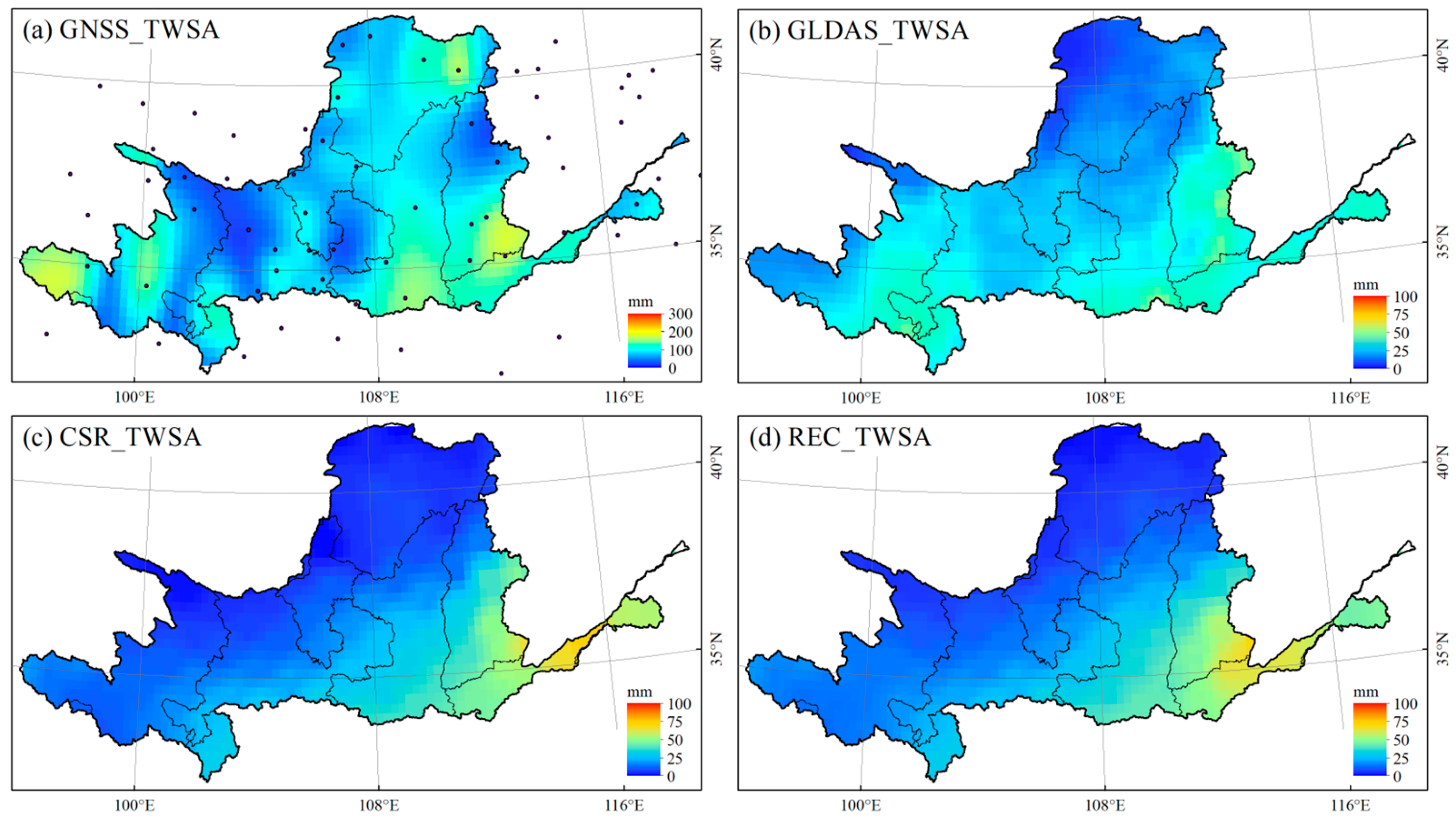
4.1. Temporal and Spatial Variations in TWSA in the YRB

TWSA show a consistent and continuous decreasing trend in the YRB from 2004 to 2021 (Figure 3a). JPL_TWSA is slightly lower than CSR_TWSA after 2015, but the correlation coefficient (CC) between the two is 0.96. In space, the decrease in GRACE TWSA is gradually aggravated from west to east (Figure 3b). The TWSA exhibit an increasing trend in most of the upper reaches, with a slight decrease in Shaanxi Province in the middle reaches. However, the decreasing trend is more serious in Shanxi Province and the lower reaches, especially the most serious decline at the confluence of Shanxi Province and Henan Province. Over the years, there has been a consistent rapid decline in TWSA in the YRB, but this trend has shown some moderation after 2018.

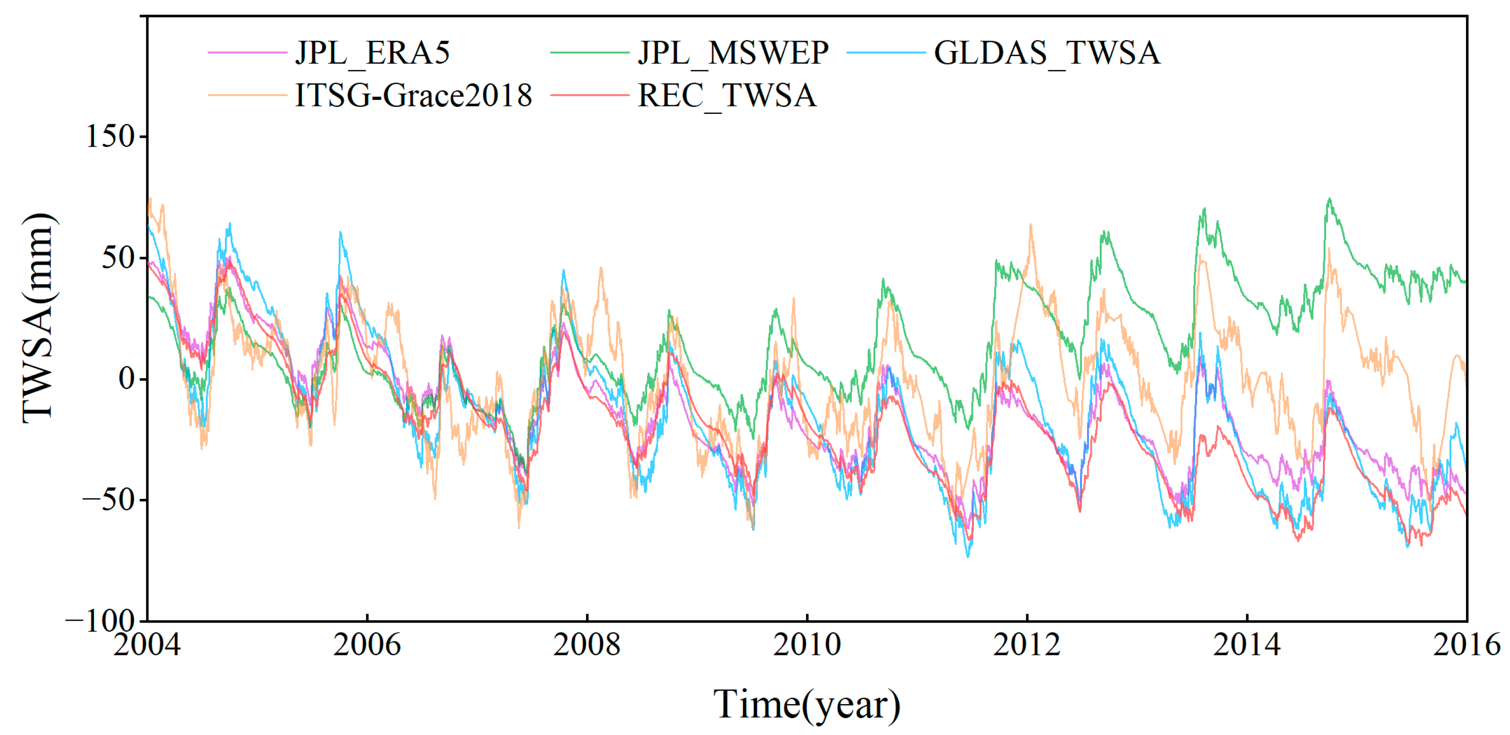
4.2. Comparison of Daily TWSA

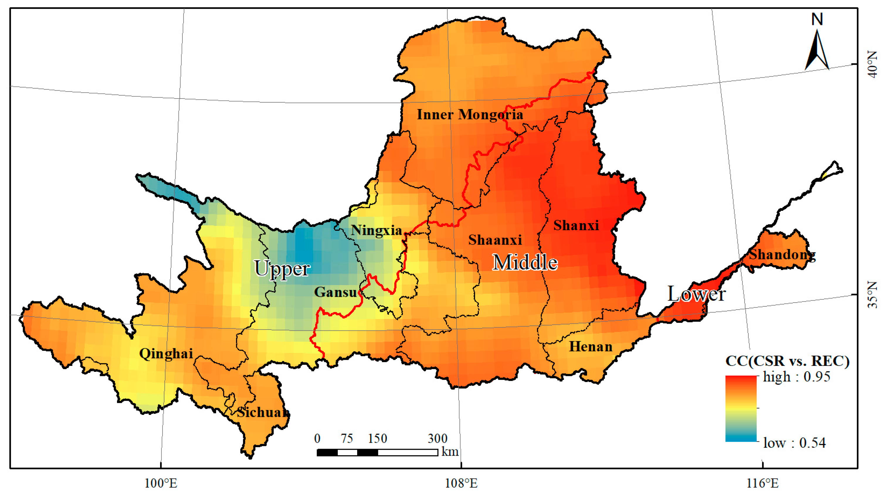
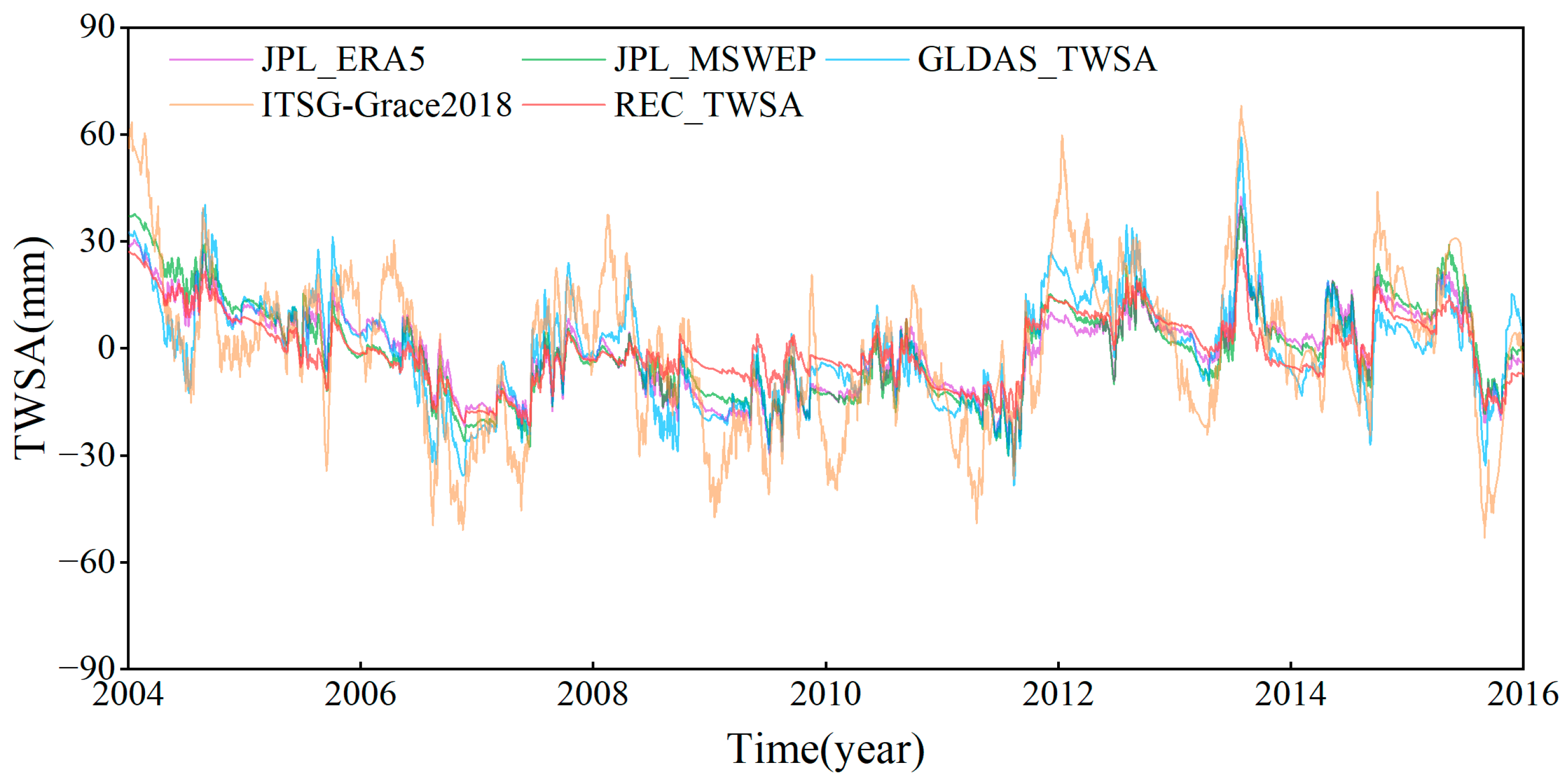
4.2.1. Evaluation of Daily TWSA for GRCAE Reconstruction

Precipitation and temperature provided by CN05.1 are used as the driving data to reconstruct the daily TWSA datasets. REC_TWSA exhibits strong agreement with the original CSR_TWSA, as evidenced by a correlation coefficient (CC) of 0.94 between their monthly averaged values. An uncertainty assessment of the reconstructed data using the Three-Cornered Hat (TCH) method [72] demonstrated that REC_TWSA exhibits an uncertainty of 9.04 mm, slightly higher than CSR_TWSA (6.80 mm) but lower than JPL_TWSA.
CSR_TWSA displays pronounced periodic variability in the YRB (Figure 4), with anomalous peaks in 2013 and troughs in 2016 [73,74]. While the reconstruction successfully replicates both the periodic oscillations and long-term declining trend of TWSA, it slightly underestimates the magnitude of TWSA fluctuations during these two extreme periods. Two factors may contribute to these minor discrepancies: (1) The original GRACE data have a monthly temporal resolution, which inherently smooths sub-monthly hydrological signals. This characteristic makes it challenging for statistical downscaling techniques to fully resolve the daily variability associated with extreme hydrological events; (2) Observational uncertainties or spatially coarse resolution in the meteorological driving data under extreme conditions may reduce TWSA reconstruction fidelity. The validity of REC_TWSA will be further evaluated against independent daily TWSA datasets in subsequent analyses.
Figure 5 shows that the reconstruction quality is well characterized for each grid in the YRB. The CC is greater than 0.54 (p < 0.05) between the CSR_TWSA and reconstructed daily TWSA and exceeds 0.8 in 71% of the regions. The reconstructed quality is relatively poor only in the upper reaches of the YRB, which is mainly due to the low vegetation cover and serious desertification in that area, resulting in a larger gap between the REC_TWSA and the CSR_TWSA.
Based on the temporal coverage of the respective datasets, the daily REC_TWSA evaluation period is determined to span from 2004 to 2015. The daily TWSA products across exhibit a high degree of consistency before 2008, with differences primarily observed in the amplitudes of peaks and troughs (Figure 6). Specifically, the peaks of GLDAS_TWSA are more prominent than the others, while the troughs of ITSG-Grace2018 are lower relative to the others. However, since 2008, the JPL_MSWEP and ITSG-Grace2018 products have become significantly more different from the others. Although there is still consistency in their seasonal variation, the trends are quite different from the marked declines exhibited by the others. An uncertainty analysis of the three datasets (excluding JPL_MSWEP and ITSG-Grace2018) demonstrated that REC_TWSA exhibits the lowest uncertainty of 5.10 mm among the three datasets.
The effectiveness of the methodology can be demonstrated further by removing trend and seasonal components. Figure 7 displays the time series of different daily TWSA products after the removal of trend and seasonal components. The REC_TWSA time series shows a high consistency with all other daily TWSA products. In particular, there is a significant similarity with the two Humphrey reconstructions, and a relatively large difference with ITSG-Grace2018.
Figure 8 displays the correlation of different daily TWSA products in the YRB. The CC is as high as 0.95 between REC_TWSA and JPL_ERA5 as well as GLDAS_TWSA products, and a lower correlation with the other products, especially the JPL_MSWEP, is noted (Figure 8a). After removing the trend and seasonal terms, the correlation decreases for those products that are highly correlated with REC_TWSA, but the CC value is still above 0.84. Meanwhile, the CC is significantly increased from 0.01 to 0.92 between REC_TWSA and JPL_MSWEP. Despite significant changes in correlations among datasets after removing trend and seasonal components, the REC_TWSA maintains relatively high correlations with most other products. Humphrey and Gudmundsson [22] have pointed out that the long-term trends of JPL_ERA5 and JPL_MSWEP need to be carefully considered when using them, potentially explaining the differences observed between JPL_MSWEP and REC_TWSA. Overall, the REC_TWSA maintains excellent correlation with the other data on time series fluctuations and is especially closer to CSR_TWSA. It also shows a high correlation with CSR_TWSA on spatial variations.

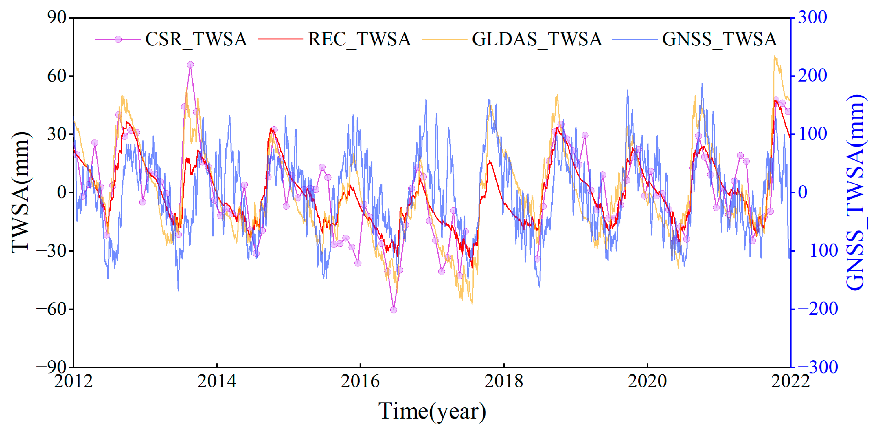
4.2.2. Evaluation of Daily TWSA for GNSS Inversion

The TWSA product from GNSS (GNSS_TWSA) exhibits high consistency in periodic variations with CSR_TWSA, GLDAS_TWSA (CC value of 0.51), and REC_TWSA (CC value of 0.58) (Figure 9). The four datasets reach maximum and minimum values around October and June each year. GNSS_TWSA displays higher annual amplitudes compared to other datasets. Nevertheless, these data can monitor regions with substantial TWSA variations in the middle and lower reaches of the YRB (Figure 10). The dots in Figure 10a represent the original GNSS stations, which are distributed uniformly in the YRB, indicating the reliability of the inversion data. The spatial amplitude of GNSS aligns most closely with GLDAS, detecting pronounced TWSA changes in the upper reaches. The maximum annual amplitudes for GNSS, GLDAS, GRACE, and reconstructed data are 183 mm, 52 mm, 72 mm, and 71 mm, respectively. While GNSS shows considerable spatial differences compared to other datasets, disparities in certain regions are considered normal due to model variations. It is important to note that changes in GNSS station density can impact the inverted TWSA, thus cautious consideration is required when utilizing this inversion technique in sparse station areas.
Two different datasets and methods are utilized to invert daily TWSA in this study. In contrast, GRACE reconstruction is superior because it provides a longer time series with a long-term linear trend. GNSS_TWSA captures only seasonal variations and has a larger annual amplitude compared to the other datasets. However, GNSS inversion results may outperform GRACE in some densely monitored areas [31,66]. Therefore, REC_TWSA is employed to study the drought conditions in the YRB.

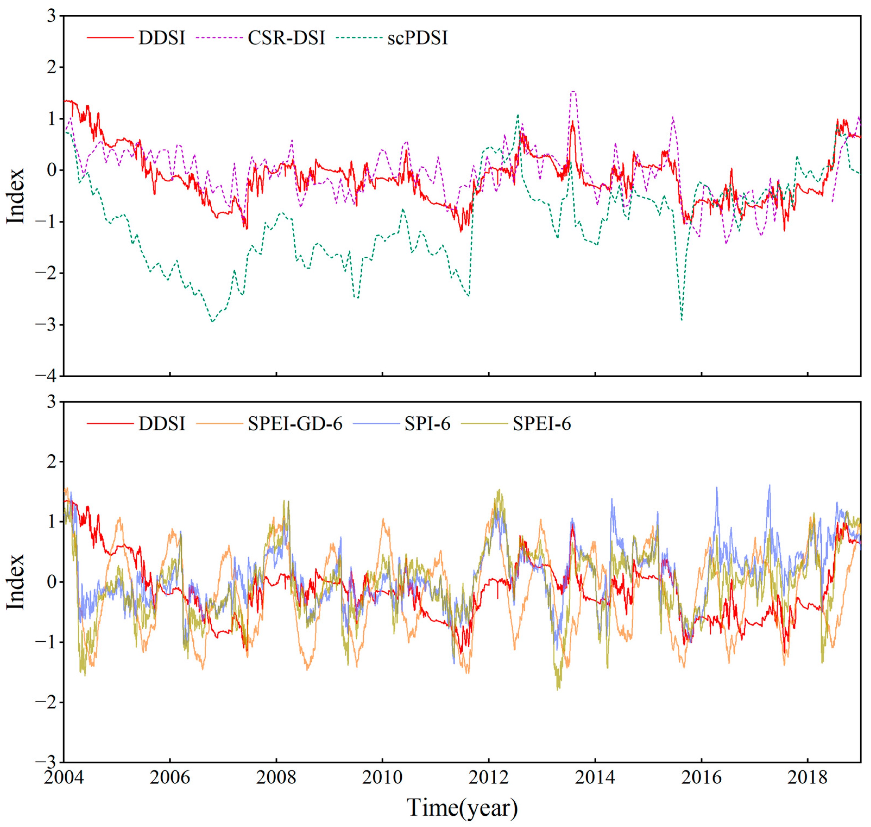
4.3. Evaluation of DDSI in the YRB

4.3.1. Temporal Variation of Drought in the YRB

A total of four drought events are monitored using the traditional DSI, and five drought events are monitored using the DDSI between 2004 and 2021 (Figure 11). The first two drought events monitored by DDSI are separated by only two days, which occurred from 14 September 2006 to 16 March 2007 and from 19 March 2007 to 17 June 2007, separately. This indicates a slight alleviation of drought in the middle of March in the YRB, resulting in the absence of a drought signal in the monthly DSI for March. Although the DSI was below the drought threshold for the four months before and after, it failed to be recorded as a drought event. Drought events are also detected by the monthly scPDSI, but there may be a tendency to overestimate drought events. Under the classification criteria of the scPDSI, which defines drought conditions when the index falls below −1, the scPDSI detected a three-year drought spanning 2005–2008, demonstrating inconsistencies with drought records documented in official bulletins. While other drought events identified using scPDSI broadly align temporally with those captured by the DDSI, its coarse temporal resolution limits its capacity to resolve finer-scale drought dynamics.
Drought is assessed from different perspectives with different drought indices, and there are correlations between them, but also differences. This is found by comparing the reconstructed DDSI with other daily drought indices. The SPEI-GD-6 can only relatively reflect the severity of drought in a given year and cannot accurately judge drought events. Under its classification criteria for drought identification, the SPEI-GD-6 index detected drought events nearly every year. While drought periods identified by the DDSI are corroborated by daily SPI-6 and SPEI-6 indices, these indices also demonstrate limitations in conclusively determining the most severe drought year, with multiple drought events detected during the study period. Furthermore, as these indices are derived from station-averaged data within the YRB, their spatial resolution (constrained by station density) impacts the precision of basin-wide drought dynamics assessment. In summary, the DDSI can more accurately monitor the specific start and end dates of drought events at the basin scale.
Two consecutive drought events occurred from 2006 to 2007, with only a two-day interval between them (Table 2). In particular, the drought event is the longest occurring with the highest drought severity and intensity from 30 October 2010 to 10 September 2011. Additionally, the drought event detected in 2015 lasted for 295 days, second only to the drought event from 2010 to 2011 (361 days). Furthermore, the fifth drought event was observed three months later, and the drought was prolonged. There is a risk of continuous drought events in the YRB within a short period.

4.3.2. Spatial Distribution of Peak Drought Events

When the DDSI minimum occurs, it is considered to have reached the peak of this drought event. The YRB has experienced five drought events in the period from 2004 to 2021. Figure 12 shows the spatial distribution of drought at the time of occurrence of the lowest DDSI values for the five drought events.
The drought was most severe and widespread on 20 June 2011, with major levels of D3 (extreme drought) and D4 (exceptional drought) covering 36.14% of the YRB. On 3 October 2016, the DDSI had the highest number of regions with drought level D4 (exceptional drought) of all drought events, and the drought-affected regions were mainly concentrated in the western and southern areas of the YRB. Additionally, the northern portion of the basin was not covered by drought, resulting in a relatively moderate overall drought intensity (−0.97) for the entire basin.
Considering the spatial distribution during peak periods of historical drought events, the frequency of stronger droughts is extremely high in the eastern part of Gansu Province and the western part of Shaanxi Province, and the drought level can reach D3 (extreme drought) and D4 (exceptional drought).

5. Discussion

5.1. Spatial Distribution of the Extreme Drought in the YRB During 2010–2011

To investigate the spatiotemporal characteristics of this extreme drought event, the period from 30 October 2010 to 10 September 2011 (Figure 13) is classified as the most severe episode based on its unprecedented duration and spatial extent of drought coverage. Specifically, the drought was more severe in the southern part of Gansu Province and the southern part of the Inner Mongolia Autonomous Region on 30 May 2011, which resulted in the formation of two drought centers. Afterward, the drought expanded from the centers to the surrounding areas, and the peak of the drought was reached on 20 June. Meantime, drought severity increased in the center, while drought level and coverage increased rapidly in the Gansu and Shaanxi borders as well as in Shanxi Province. The percentage of areas peaked with drought levels of D3 and D4 (Figure 14).
After that, the drought extent did not decrease, but the drought level decreased slightly. The drought level increased again on 30 June, with the most severe areas still in southern Gansu Province and southern Inner Mongolia Autonomous Region. Compared with 20 June, the drought was more concentrated on 30 June, and the drought was higher in coverage and level in the Inner Mongolia Autonomous Region. After 5 July, the drought was gradually relieved in most of the YRB, but the drought still existed and continued for a long time in the Inner Mongolia Autonomous Region. The “2011 Bulletin of Flood and Drought Disaster in China” [75] also describes the existence of spring, summer, and autumn droughts in Inner Mongolia, which is consistent with the drought process in this study.

5.2. Impact of Climate and Human Factors for Drought

The primary objective of reconstructing CWSA is to analyze the influencing factors of drought, specifically to determine whether droughts in the YRB are caused by human activities or climate change. If the linear trend of TWSA exceeds CWSA, it indicates the presence of human factors causing an increase in TWSA; conversely, it indicates the presence of human factors that are causing TWSA to decrease. The primary reason for the decline in TWSA is excessive groundwater extraction.
From 2004 to 2021, the TWSA in the YRB exhibited a sustained declining trend (−5.32 mm/yr, Figure 15). In contrast, the CWSA showed a slight increase trend (0.13 mm/yr). The linear trend of TWSA is significantly lower than that of CWSA, and the discrepancy arises from the human factors. Otherwise, the trend in GWSA (−7.41 mm/yr) is consistent with the trend in HWSA (−5.45 mm/yr), and the CC between them is 0.81. This suggests that the TWSA of YRB are dominated by human activity and that human factors impact TWSA primarily through GWSA.
Compared with the upper and middle reaches, the lower reaches have the sharpest decreasing trend in TWSA, HWSA, and GWSA (Table 3). The main reason for this is that the lower reaches are closer to the Haihe River basin, where human influences are much greater [76]. The closer the area is to the North China Plain, the greater the TWSA decline rate, and the greater the efficiency of human factors. In addition, reduced precipitation also contributed to the decrease in TWSA in the lower reaches. The relatively small area of the lower reaches combined with the spatial resolution limitations of GRACE data may lead to greater uncertainties in water storage estimates for the region. As shown in Table 3, the linear trend errors in this area are significantly larger than those in other regions, yet the long-term declining trend of water storage remains evident. Except for CWSA, all other water storage components in the YRB and its sub-basins exhibit decreasing trends with varying magnitudes, particularly the drastic decline in HWSA within the mid-lower reaches. This indicates substantial human impacts on basin water storage variations, thereby indirectly affecting drought occurrences.
A comprehensive analysis of water storage anomalies in the upper, middle, and lower reaches of the YRB suggests that climate factors play a relatively minor role in the decline in TWSA. The decline in TWSA is primarily driven by human influences, with GWSA identified as the primary human factor. Human activities have significantly impacted drought evolution in the Yellow River Basin, particularly in the mid-lower reaches where water resource depletion has reached critical levels, calling for increased scientific attention.

6. Conclusions

A GRACE reconstruction method is used to obtain daily TWSA products in this study that are used to construct DDSI to explore the drought events in the YRB in detail. In addition, the CWSA reconstruction model is utilized to isolate the climate and human influences on TWSA. The main conclusions are as follows:
(1) The time series are highly consistent between CSR_TWSA and JPL_TWSA in the YRB from 2004 to 2021, with a CC of 0.96, and both are within the error range. There is a severe decreasing trend for TWSA in the middle and lower reaches spatially, especially in the southeastern part of Shanxi Province and Henan Province.
(2) The CC is 0.94 for REC_TWSA and CSR_TWSA in the time series and is spatially greater than 0.54 with about 71% of the region above 0.8. REC_TWSA also maintains a high correlation with the other daily TWSA datasets in terms of time series variation. GNSS_TWSA is consistent with GLDAS_TWSA and REC_TWSA in the cycle variation, and it can monitor the drastic changes of TWSA in the middle and lower reaches of the YRB. However, the annual amplitude of GNSS_TWSA is limited by the amount of original data and the point distribution. The GRACE reconstruction method is better than others in acquiring daily TWSA.
(3) The DDSI exhibits similar peaks and valleys as other drought indices and has recognized five drought events from 2004 to 2021. The drought event is the longest (316 days) and most severe (−238.31) from 2010 to 2011. The southern part of the Inner Mongolia Autonomous Region and the middle reaches of the YRB are prone to drought according to the spatial distribution of historical drought events. In total, 36.14% of the area reached drought levels of D3 and D4 on 20 June 2011, and the eastern part of Gansu Province and the Inner Mongolia Autonomous Region suffered from the most severe drought. The drought conditions obtained using the DDSI are consistent with the government bulletin.
(4) Human factors are the major cause of the decline in TWSA in the YRB, which have influenced drought occurrences. The decreasing trends of HWSA and GWSA have a strong consistency, with a CC value as high as 0.81, which indicates that the depletion of TWSA is mainly attributed to excessive groundwater extraction by humans.
This study employs model-based reconstruction to delineate daily spatiotemporal drought dynamics in the Yellow River Basin, quantifying climate and human contributions to drought, thereby offering actionable insights for localized drought monitoring and adaptive water governance.

Author Contributions

Conceptualization, Y.L.; methodology, W.Y.; validation, W.Z. and W.Y.; formal analysis, Y.L.; investigation, Y.L. and S.N.; resources, W.Z.; data curation, W.Y.; writing—original draft preparation, Y.L.; writing—review and editing, S.N. and W.L.; visualization, W.L.; supervision, H.Z. and W.L.; project administration, W.Y.; funding acquisition, W.Z. and H.Z. All authors have read and agreed to the published version of the manuscript.

Funding

This work was supported in part by the National Natural Science Foundation of China (Grant No. U23A2015, 42274119), in part by the National Key Research and Development Plan Key Special Projects of Science and Technology Military Civil Integration (Grant No. 2022YFF1400500), the Young Teachers Development Fund (Science and Engineering Category) of Harbin Institute of Technology (Weihai) (Grant No. IDGA10002224), and in part by the Scientific Research Project of ‘Double First-Class’ Construction Project of Surveying and Mapping Science and Technology Discipline in Henan Province (Grant No. BZCG202303).

Data Availability Statement

No new data were created or analyzed in this study. Data sharing is not applicable to this article.

Acknowledgments

The authors very appreciate the CSR and JPL for providing the GRACE mascon solution, the Climate Change Research Center of the Chinese Academy of Science for providing the CN05.1 dataset, NASA for providing the GLDAS datasets, and the China Earthquake Science Data Center for providing the GNSS observation dataset.

Conflicts of Interest

The authors declare no conflicts of interest.

References

  1. Tran, T.-N.-D.; Lakshmi, V. Enhancing Human Resilience against Climate Change: Assessment of Hydroclimatic Extremes and Sea Level Rise Impacts on the Eastern Shore of Virginia, United States. Sci. Total Environ. 2024, 947, 174289. [Google Scholar] [CrossRef] [PubMed]
  2. Kafi, K.M.; Ponrahono, Z. Advances in Weather and Climate Extreme Studies: A Systematic Comparative Review. Discov. Geosci. 2024, 2, 66. [Google Scholar] [CrossRef]
  3. Hermans, K.; McLeman, R. Climate Change, Drought, Land Degradation and Migration: Exploring the Linkages. Curr. Opin. Environ. Sustain. 2021, 50, 236–244. [Google Scholar] [CrossRef]
  4. Nandgude, N.; Singh, T.P.; Nandgude, S.; Tiwari, M. Drought Prediction: A Comprehensive Review of Different Drought Prediction Models and Adopted Technologies. Sustainability 2023, 15, 11684. [Google Scholar] [CrossRef]
  5. Tapley, B.D.; Bettadpur, S.; Ries, J.C.; Thompson, P.F.; Watkins, M.M. GRACE Measurements of Mass Variability in the Earth System. Science 2004, 305, 503–505. [Google Scholar] [CrossRef]
  6. Elhaddad, H.; Sultan, M.; Yan, E.; Abdelmohsen, K.; Mohammad, A.T.; Badawy, A.; Karimi, H.; Saleh, H.; Emil, M.K. Optimization of Floodwater Redistribution from Lake Nasser Could Recharge Egypt’s Aquifers and Mitigate Its Excessive Floods. Commun. Earth Environ. 2024, 5, 385. [Google Scholar] [CrossRef]
  7. Luo, Z.; Yao, C.; Li, Q.; Huang, Z. Terrestrial Water Storage Changes over the Pearl River Basin from GRACE and Connections with Pacific Climate Variability. Geod. Geodyn. 2016, 7, 171–179. [Google Scholar] [CrossRef]
  8. Yao, C.; Luo, Z.; Wang, H.; Li, Q.; Zhou, H. GRACE-Derived Terrestrial Water Storage Changes in the Inter-Basin Region and Its Possible Influencing Factors: A Case Study of the Sichuan Basin, China. Remote Sens. 2016, 8, 444. [Google Scholar] [CrossRef]
  9. Meng, F.; Su, F.; Li, Y.; Tong, K. Changes in Terrestrial Water Storage During 2003–2014 and Possible Causes in Tibetan Plateau. J. Geophys. Res. 2019, 124, 2909–2931. [Google Scholar] [CrossRef]
  10. Xu, G.; Liu, S.; Cheng, S.; Zhang, Y.; Wu, X.; Wu, Y. Quantifying the 2022 Drought and Spatiotemporal Evolution of TWSA in the Dongting Lake Basin over the Past Two Decades. Geod. Geodyn. 2024, 15, 516–527. [Google Scholar] [CrossRef]
  11. Ramillien, G.; Frappart, F.; Guntner, A.; Ngo-Duc, T.; Cazenave, A.; Laval, K. Time Variations of the Regional Evapotranspiration Rate from Gravity Recovery and Climate Experiment (GRACE) Satellite Gravimetry. Water Resour. Res. 2006, 42, W10403. [Google Scholar] [CrossRef]
  12. Syed, T.H.; Famiglietti, J.S.; Rodell, M.; Chen, J.; Wilson, C.R. Analysis of Terrestrial Water Storage Changes from GRACE and GLDAS. Water Resour. Res. 2008, 44, W02433. [Google Scholar] [CrossRef]
  13. Yeh, P.J.-F.; Swenson, S.C.; Famiglietti, J.S.; Rodell, M. Remote Sensing of Groundwater Storage Changes in Illinois Using the Gravity Recovery and Climate Experiment (GRACE). Water Resour. Res. 2006, 42, W12203. [Google Scholar] [CrossRef]
  14. Scanlon, B.R.; Longuevergne, L.; Long, D. Ground Referencing GRACE Satellite Estimates of Groundwater Storage Changes in the California Central Valley, USA. Water Resour. Res. 2012, 48, W04520. [Google Scholar] [CrossRef]
  15. Zhang, G.; Zheng, W.; Yin, W.; Lei, W. Improving the Resolution and Accuracy of Groundwater Level Anomalies Using the Machine Learning-Based Fusion Model in the North China Plain. Sensors 2020, 21, 46. [Google Scholar] [CrossRef]
  16. Wang, X.; Zheng, W.; Yin, W.; Xu, K.; Zhang, H.; Lei, W. Enhancing Spatial Resolution of Drought Monitoring through a Novel Random Forest-Based GRACE Drought Index: A Case Study in Central Yunnan. Geocarto Int. 2024, 39, 2387784. [Google Scholar] [CrossRef]
  17. Yin, W.; Hu, L.; Zhang, M.; Wang, J.; Han, S. Statistical Downscaling of GRACE-Derived Groundwater Storage Using ET Data in the North China Plain. J. Geophys. Res. Atmos. 2018, 123, 5973–5987. [Google Scholar] [CrossRef]
  18. Chen, Z.; Zheng, W.; Yin, W.; Li, X.; Zhang, G.; Zhang, J. Improving the Spatial Resolution of GRACE-Derived Terrestrial Water Storage Changes in Small Areas Using the Machine Learning Spatial Downscaling Method. Remote Sens. 2021, 13, 4760. [Google Scholar] [CrossRef]
  19. Chu, J.; Su, X.; Zhang, T.; Lei, Y.; Jiang, T.; Wu, H.; Wang, Q. Comparison of Three Spatial Downscaling Concepts of GRACE Data Using Random Forest Model. J. Lake Sci. 2024, 36, 951–962. [Google Scholar] [CrossRef]
  20. Gouweleeuw, B.T.; Kvas, A.; Gruber, C.; Gain, A.K.; Mayer-Gürr, T.; Flechtner, F.; Güntner, A. Daily GRACE Gravity Field Solutions Track Major Flood Events in the Ganges–Brahmaputra Delta. Hydrol. Earth Syst. Sci. 2018, 22, 2867–2880. [Google Scholar] [CrossRef]
  21. Kvas, A.; Behzadpour, S.; Ellmer, M.; Klinger, B.; Strasser, S.; Zehentner, N.; Mayer-Gürr, T. ITSG-Grace2018: Overview and Evaluation of a New GRACE-Only Gravity Field Time Series. J. Geophys. Res. Solid Earth 2019, 124, 9332–9344. [Google Scholar] [CrossRef]
  22. Humphrey, V.; Gudmundsson, L. GRACE-REC: A Reconstruction of Climate-Driven Water Storage Changes over the Last Century. Earth Syst. Sci. Data 2019, 11, 1153–1170. [Google Scholar] [CrossRef]
  23. Xiao, C.; Zhong, Y.; Feng, W.; Gao, W.; Wang, Z.; Zhong, M.; Ji, B. Monitoring the Catastrophic Flood with GRACE-FO and Near-Real-Time Precipitation Data in Northern Henan Province of China in July 2021. IEEE J. Sel. Top. Appl. Earth Obs. Remote Sens. 2023, 16, 89–101. [Google Scholar] [CrossRef]
  24. Wang, L.; Zhang, M.; Yin, W.; Li, Y.; Hu, L.; Fan, L. Improved Drought Characteristics in the Pearl River Basin Based on Reconstructed GRACE Solution with Enhanced Temporal Resolution. Remote Sens. 2023, 15, 4849. [Google Scholar] [CrossRef]
  25. Van Dam, T.M.; Wahr, J. Modeling Environment Loading Effects: A Review. Phys. Chem. Earth 1998, 23, 1077–1087. [Google Scholar] [CrossRef]
  26. Wang, L.; Chen, C.; Zou, R.; Du, J.; Chen, X. Using GPS and GRACE to Detect Seasonal Horizontal Deformation Caused by Loading of Terrestrial water: A Case Study in the Himalayas. Chin. J. Geophys. 2014, 57, 1792–1804. [Google Scholar] [CrossRef]
  27. Ding, Y.; Huang, D.; Shi, Y.; Jiang, Z.; Chen, T. Determination of Vertical Surface Displacements in Sichuan Using GPS and GRACE Measurements. Chin. J. Geophys. 2018, 61, 4777–4788. [Google Scholar] [CrossRef]
  28. Knappe, E.; Bendick, R.; Martens, H.R.; Argus, D.F.; Gardner, W.P. Downscaling Vertical GPS Observations to Derive Watershed-Scale Hydrologic Loading in the Northern Rockies. Water Resour. Res. 2019, 55, 391–401. [Google Scholar] [CrossRef]
  29. Han, S.; Razeghi, S.M. GPS Recovery of Daily Hydrologic and Atmospheric Mass Variation: A Methodology and Results from the Australian Continent. J. Geophys. Res. Solid Earth 2017, 122, 9328–9343. [Google Scholar] [CrossRef]
  30. Jiang, Z.; Hsu, Y.-J.; Yuan, L.; Cheng, S.; Li, Q.; Li, M. Estimation of Daily Hydrological Mass Changes Using Continuous GNSS Measurements in Mainland China. J. Hydrol. 2021, 598, 126349. [Google Scholar] [CrossRef]
  31. Peng, Y.; Chen, G.; Chao, N.; Wang, Z.; Wu, T.; Luo, X. Detection of Extreme Hydrological Droughts in the Poyang Lake Basin during 2021–2022 Using GNSS-Derived Daily Terrestrial Water Storage Anomalies. Sci. Total Environ. 2024, 919, 170875. [Google Scholar] [CrossRef] [PubMed]
  32. She, D.; Xia, J.; Du, H.; Wan, L. Spatio-temporal Analysis and Multi-variable Statistical Models of Extreme Drought Events in Yellow River Basin, China. J. Basic Sci. Eng. 2012, 20, 15–29. Available online: https://kns.cnki.net/KCMS/detail/detail.aspx?dbcode=CJFQ&dbname=CJFD2012&filename=YJGX2012S1001 (accessed on 2 September 2024).
  33. Cao, C.; Ren, L.; Liu, Y.; Jiang, S.; Zhang, L.; Zhang, L. Spatial-Temporal Characteristics of Drought of the Yellow River Basin Based on Joint Drought Index. Yellow River 2019, 41, 51–56. [Google Scholar] [CrossRef]
  34. Qu, W.; Jin, Z.; Zhang, Q.; Gao, Y.; Zhang, P. Drought characteristics of the Yellow River basin from 2002 to 2020 revealed by GRACE and GRACE Follow-On data. Acta Geod. Cartogr. Sinica 2023, 52, 714–724. [Google Scholar] [CrossRef]
  35. Xie, X.; Xing, M.; Wang, L.; Xu, G.; Wen, H. Using GRACE/GRACE-FO Gravity Satellite to Detect the Water Storage Capacity and the Possibility of Extreme Climate in the Yellow River Basin. J. Geod. Geodyn. 2022, 42, 1269–1275. [Google Scholar] [CrossRef]
  36. Yuan, Z.; Zhang, Z.; Yan, J.; Liu, J.; Hu, Z.; Wang, Y.; Cai, M. Spatiotemporal characteristics of different grades of precipitation in Yellow River Basin from 1960 to 2020. Arid Zone Res. 2024, 41, 1259–1271. [Google Scholar] [CrossRef]
  37. Ji, X.; Liu, M.; Wu, X.; Ding, Y.; Zhu, Y. Spatiotemporal variation characteristics of rainfall erosivity in the Yellow River Basin from 1961 to 2019. Trans. Chin. Soc. Agric. Eng. 2022, 38, 136–145. [Google Scholar] [CrossRef]
  38. Li, C.; Yu, W.; Zhang, X. Spatio-Temporal Patterns of High-Quality Urbanization Development under Water Resource Constraints and Their Key Drivers: A Case Study in the Yellow River Basin, China. Ecol. Indic. 2024, 166, 112441. [Google Scholar] [CrossRef]
  39. Save, H.; Bettadpur, S.; Tapley, B.D. High-resolution CSR GRACE RL05 Mascons. J. Geophys. Res. 2016, 121, 7547–7569. [Google Scholar] [CrossRef]
  40. Wiese, D.N.; Landerer, F.W.; Watkins, M.M. Quantifying and Reducing Leakage Errors in the JPL RL05M GRACE Mascon Solution. Water Resour. Res. 2016, 52, 7490–7502. [Google Scholar] [CrossRef]
  41. Li, B.; Rodell, M.; Kumar, S.; Beaudoing, H.K.; Getirana, A.; Zaitchik, B.F.; Goncalves, L.G.; Cossetin, C.; Bhanja, S.; Mukherjee, A.; et al. Global GRACE Data Assimilation for Groundwater and Drought Monitoring: Advances and Challenges. Water Resour. Res. 2019, 55, 7564–7586. [Google Scholar] [CrossRef]
  42. Li, B.; Beaudoing, H.; Rodell, M. NASA/GSFC/HSL, GLDAS Catchment Land Surface Model L4 Daily 0.25 × 0.25 Degree GRACE-DA1 V2.2, Greenbelt, Maryland, USA, Goddard Earth Sciences Data and Information Services Center (GES DISC). Available online: https://disc.gsfc.nasa.gov/datasets/GLDAS_CLSM025_DA1_D_2.2/summary (accessed on 14 April 2024).
  43. Mayer-Gürr, T.; Behzadpur, S.; Ellmer, M.; Kvas, A.; Klinger, B.; Strasser, S.; Zehentner, N. ITSG-Grace2018—Monthly, Daily and Static Gravity Field Solutions from GRACE. GFZ Data Serv. Available online: https://www.tugraz.at/institute/ifg/downloads/gravity-field-models/itsg-grace2018 (accessed on 6 June 2024).
  44. Xu, Y.; Gao, X.; Shen, Y.; Xu, C.; Shi, Y.; Giorgi, F. A Daily Temperature Dataset over China and Its Application in Validating a RCM Simulation. Adv. Atmos. Sci. 2009, 26, 763–772. [Google Scholar] [CrossRef]
  45. Wu, J.; Gao, X. A Gridded Daily Observation Dataset over China Region and Comparison with the Other Datasets. Chin. J. Geophys. 2013, 56, 1102–1111. [Google Scholar] [CrossRef]
  46. Wu, J.; Gao, X.; Giorgi, F.; Chen, D. Changes of Effective Temperature and Cold/Hot Days in Late Decades over China Based on a High Resolution Gridded Observation Dataset. Int. J. Climatol. 2017, 37, 788–800. [Google Scholar] [CrossRef]
  47. Nie, S.; Zheng, W.; Yin, W.; Zhong, Y.; Shen, Y.; Li, K. Improved the Characterization of Flood Monitoring Based on Reconstructed Daily GRACE Solutions over the Haihe River Basin. Remote Sens. 2023, 15, 1564. [Google Scholar] [CrossRef]
  48. Muñoz Sabater, J. ERA5-Land Monthly Averaged Data from 1950 to Present. Copernicus Climate Change Service (C3S) Climate Data Store (CDS). Available online: https://cds.climate.copernicus.eu/cdsapp#!/dataset/reanalysis-era5-land-monthly-means?tab=form (accessed on 2 May 2024).
  49. Jiao, D.; Xu, N.; Yang, F.; Xu, K. Evaluation of Spatial-Temporal Variation Performance of ERA5 Precipitation Data in China. Sci. Rep. 2021, 11, 17956. [Google Scholar] [CrossRef]
  50. Zhao, P.; He, Z. A First Evaluation of ERA5-Land Reanalysis Temperature Product over the Chinese Qilian Mountains. Front. Earth Sci. 2022, 10, 907730. [Google Scholar] [CrossRef]
  51. Wells, N.; Goddard, S.; Hayes, M.J. A Self-Calibrating Palmer Drought Severity Index. J. Clim. 2004, 17, 2335–2351. [Google Scholar] [CrossRef]
  52. Van Der Schrier, G.; Barichivich, J.; Briffa, K.R.; Jones, P.D. A scPDSI-based Global Data Set of Dry and Wet Spells for 1901–2009. J. Geophys. Res. Atmos. 2013, 118, 4025–4048. [Google Scholar] [CrossRef]
  53. Yang, Q.; Li, M.; Zheng, Z.; Ma, Z. Regional applicability of seven meteorological drought indices in China. Sci. China Earth Sci. 2017, 47, 337–353. [Google Scholar] [CrossRef]
  54. Wang, Q.; Zeng, J.; Qi, J.; Zhang, X.; Zeng, Y.; Shui, W.; Xu, Z.; Zhang, R.; Wu, X.; Cong, J. A Multi-Scale Daily SPEI Dataset for Drought Characterization at Observation Stations over Mainland China from 1961 to 2018. Earth Syst. Sci. Data 2021, 13, 331–341. [Google Scholar] [CrossRef]
  55. Wang, Q.; Zhang, R.; Qi, J.; Zeng, J.; Wu, J.; Shui, W.; Wu, X.; Li, J. An Improved Daily Standardized Precipitation Index Dataset for Mainland China from 1961 to 2018. Sci. Data 2022, 9, 124. [Google Scholar] [CrossRef] [PubMed]
  56. Liu, X.; Yu, S.; Yang, Z.; Dong, J.; Peng, J. The First Global Multi-Timescale Daily SPEI Dataset from 1982 to 2021. Sci. Data 2024, 11, 223. [Google Scholar] [CrossRef]
  57. Beaudoing, H.; Rodell, M. GLDAS Noah Land Surface Model L4 Monthly 0.25 × 0.25 Degree V2.1, Greenbelt, Maryland, USA, Goddard Earth Sciences Data and Information Services Center (GES DISC). Available online: https://disc.gsfc.nasa.gov/datasets/GLDAS_NOAH025_M_2.1/summary (accessed on 5 August 2024).
  58. Rodell, M.; Houser, P.R.; Jambor, U.; Gottschalck, J.; Mitchell, K.; Meng, C.-J.; Arsenault, K.; Cosgrove, B.; Radakovich, J.; Bosilovich, M.; et al. The Global Land Data Assimilation System. Bull. Amer. Meteor. Soc. 2004, 85, 381–394. [Google Scholar] [CrossRef]
  59. Hosseini-Moghari, S.-M.; Araghinejad, S.; Ebrahimi, K.; Tang, Q.; AghaKouchak, A. Using GRACE Satellite Observations for Separating Meteorological Variability from Anthropogenic Impacts on Water Availability. Sci. Rep. 2020, 10, 15098. [Google Scholar] [CrossRef]
  60. Kraner, M.L.; Holt, W.E.; Borsa, A.A. Seasonal Nontectonic Loading Inferred from cGPS as a Potential Trigger for the M6.0 South Napa Earthquake. J. Geophys. Res. Solid Earth 2018, 123, 5300–5322. [Google Scholar] [CrossRef]
  61. Chanard, K.; Fleitout, L.; Calais, E.; Rebischung, P.; Avouac, J. Toward a Global Horizontal and Vertical Elastic Load Deformation Model Derived from GRACE and GNSS Station Position Time Series. J. Geophys. Res. Solid Earth 2018, 123, 3225–3237. [Google Scholar] [CrossRef]
  62. Jiang, Z.; Hsu, Y.-J.; Yuan, L.; Feng, W.; Yang, X.; Tang, M. GNSS2TWS: An Open-Source MATLAB-Based Tool for Inferring Daily Terrestrial Water Storage Changes Using GNSS Vertical Data. GPS Solut. 2022, 26, 114. [Google Scholar] [CrossRef]
  63. Jiang, Z.; Hsu, Y.-J.; Yuan, L.; Huang, D. Monitoring Time-Varying Terrestrial Water Storage Changes Using Daily GNSS Measurements in Yunnan, Southwest China. Remote Sens. Environ. 2021, 254, 112249. [Google Scholar] [CrossRef]
  64. Dziewonski, A.M.; Anderson, D.L. Preliminary Reference Earth Model. Phys. Earth Planet. Inter. 1981, 25, 297–356. [Google Scholar] [CrossRef]
  65. Fu, Y.; Argus, D.F.; Landerer, F.W. GPS as an Independent Measurement to Estimate Terrestrial Water Storage Variations in Washington and Oregon. J. Geophys. Res. Solid Earth 2015, 120, 552–566. [Google Scholar] [CrossRef]
  66. Hsu, Y.-J.; Fu, Y.; Bürgmann, R.; Hsu, S.-Y.; Lin, C.-C.; Tang, C.-H.; Wu, Y.-M. Assessing Seasonal and Interannual Water Storage Variations in Taiwan Using Geodetic and Hydrological Data. Earth Planet. Sci. Lett. 2020, 550, 116532. [Google Scholar] [CrossRef]
  67. Liu, X.; Feng, X.; Ciais, P.; Fu, B.; Hu, B.; Sun, Z. GRACE Satellite-Based Drought Index Indicating Increased Impact of Drought over Major Basins in China during 2002–2017. Agric. For. Meteorol. 2020, 291, 108057. [Google Scholar] [CrossRef]
  68. Cui, A.; Li, J.; Zhou, Q.; Zhu, R.; Liu, H.; Wu, G.; Li, Q. Use of a Multiscalar GRACE-Based Standardized Terrestrial Water Storage Index for Assessing Global Hydrological Droughts. J. Hydrol. 2021, 603, 126871. [Google Scholar] [CrossRef]
  69. Zhao, M.; Geruo, A.; Velicogna, I.; Kimball, J.S. Satellite Observations of Regional Drought Severity in the Continental United States Using GRACE-Based Terrestrial Water Storage Changes. J. Clim. 2017, 30, 6297–6308. [Google Scholar] [CrossRef]
  70. Deng, Z.; Wu, X.; Wang, Z.; Li, J.; Chen, X. Drought monitoring based on GRACE data in the Pearl River Basin, China. Trans. Chin. Soc. Agric. Eng. 2020, 36, 179–187. [Google Scholar] [CrossRef]
  71. Liu, B.; Zou, X.; Yi, S.; Sneeuw, N.; Cai, J.; Li, J. Identifying and Separating Climate- and Human-Driven Water Storage Anomalies Using GRACE Satellite Data. Remote Sens. Environ. 2021, 263, 112559. [Google Scholar] [CrossRef]
  72. Zhang, G.; Xu, T.; Yin, W.; Bateni, S.M.; Jun, C.; Kim, D.; Liu, S.; Xu, Z.; Ming, W.; Wang, J. A Machine Learning Downscaling Framework Based on a Physically Constrained Sliding Window Technique for Improving Resolution of Global Water Storage Anomaly. Remote Sens. Environ. 2024, 313, 114359. [Google Scholar] [CrossRef]
  73. The Ministry of Water Resources of the People’s Republic of China. 2013 Bulletin of Flood and Drought Disasters in China. p. 11. Available online: http://www.mwr.gov.cn/sj/tjgb/zgshzhgb/201612/t20161222_776091.html (accessed on 2 September 2024).
  74. The Ministry of Water Resources of the People’s Republic of China. 2016 Bulletin of Flood and Drought Disasters in China. p. 38. Available online: http://www.mwr.gov.cn/sj/tjgb/zgshzhgb/201707/t20170720_966705.html (accessed on 2 September 2024).
  75. The Ministry of Water Resources of the People’s Republic of China. 2011 Bulletin of Flood and Drought Disasters in China. p. 24. Available online: http://www.mwr.gov.cn/sj/tjgb/zgshzhgb/201612/t20161222_776089.html (accessed on 2 September 2024).
  76. Zhong, Y.; Feng, W.; Humphrey, V.; Zhong, M. Human-Induced and Climate-Driven Contributions to Water Storage Variations in the Haihe River Basin, China. Remote Sens. 2019, 11, 3050. [Google Scholar] [CrossRef]
Figure 1. Elevation and partition of the YRB.
Water 17 01245 g001
Figure 2. Flowchart for this study.
Water 17 01245 g002
Figure 3. Spatiotemporal variations of GRACE TWSA in the YRB: (a) time series of CSR_TWSA and JPL_TWSA, (b) spatial distributions of GRACE TWSA trend.
Water 17 01245 g003
Figure 4. Time series of REC_TWSA, CSR_TWSA, and precipitation in the YRB.
Water 17 01245 g004
Figure 5. Spatial correlation between CSR_TWSA and REC_TWSA in the YRB (p < 0.05).
Water 17 01245 g005
Figure 6. Time series of daily TWSA products in the YRB.
Water 17 01245 g006
Figure 7. Time series of daily TWSA products after removing trend and seasonal components.
Water 17 01245 g007
Figure 8. CC of different daily TWSA products: (a) CC of complete data; (b) CC after removing seasonal and trend components.
Water 17 01245 g008
Figure 9. Time series of GNSS_TWSA, CSR_TWSA, GLDAS_TWSA, and REC_TWSA in the YRB.
Water 17 01245 g009
Figure 10. Spatial distribution of annual amplitudes of TWSA products in the YRB.
Water 17 01245 g010
Figure 11. Time series of drought indices in the YRB.
Water 17 01245 g011
Figure 12. Spatial distribution during peak periods of historical drought events based on the DDSI.
Water 17 01245 g012
Figure 13. Spatial distribution of drought monitored by DDSI in the YRB from 30 May 2011 to 6 July 2011.
Water 17 01245 g013
Figure 14. Percentage of drought types monitored using the DDSI in the YRB from 30 May 2011 to 6 July 2011.
Water 17 01245 g014
Figure 15. Temporal evolution of water storage anomalies in the YRB: (a) Yellow River basin, (b) Upper reaches, (c) Middle reaches, (d) Lower reaches.
Water 17 01245 g015
Table 1. Classification of drought severity for different drought indices.
CategoryDescriptionDDSIscPDSISPISPEISPEI-GD
D0Mild drought−0.50 to −0.79
D1Moderate drought−0.80 to −1.29−1 to −1.99−0.5 to −0.99−0.5 to −0.99−0.5 to −0.99
D2Severe drought−1.30 to −1.59−2 to −2.99−1 to −1.49−1 to −1.49−1 to −1.49
D3Extreme drought−1.60 to −1.99−3 to −3.99−1.5 to −1.99−1.5 to −1.99−1.5 to −1.99
D4Exceptional drought−2.0 or less−4 or less−2 or less−2 or less−2 or less
Table 2. Periods of drought events detected using the DDSI.
IDPeriodPeriod (Days)Total SeverityMinimum DDSIMinimum DDSI Date
12006/9/14 to 2007/3/16184−144.55−0.932006/11/18
22007/3/19 to 2007/6/1791−73.94−1.142007/6/10
32010/10/30 to 2011/9/10316−238.31−1.22011/6/20
42015/8/12 to 2016/6/1295−206.73−1.042015/9/2
52016/8/29 to 2017/3/22206−145.29−0.972016/10/3
Table 3. Statistical analysis of linear trends in water storage anomalies in the YRB, 2004–2021.
TWSA TrendCWSA TrendHWSA TrendGWSA Trend
Yellow River basin−5.32 ± 0.290.13 ± 0.18−5.45 ± 0.23−7.41 ± 0.17
Upper reaches−1.27 ± 0.260.11 ± 0.18−1.44 ± 0.18−4.17 ± 0.14
Middle reaches−9.12 ± 0.46−0.02 ± 0.17−9.01 ± 0.44−10.52 ± 0.26
Lower reaches−24.94 ± 1.13−0.48 ± 0.44−24.39 ± 1.08−22.25 ± 0.46
Disclaimer/Publisher’s Note: The statements, opinions and data contained in all publications are solely those of the individual author(s) and contributor(s) and not of MDPI and/or the editor(s). MDPI and/or the editor(s) disclaim responsibility for any injury to people or property resulting from any ideas, methods, instructions or products referred to in the content.

