Determination of Hydrological Flood Hazard Thresholds and Flood Frequency Analysis: Case Study of Nokoue Lake Watershed

Abstract

With the impacts of climate change, floods have become increasingly frequent in recent years. Estimating flood hazard thresholds and peak floodwater levels based on flood frequency analysis is crucial for anticipating and preparing for potential flooding events. This study aims to estimate flood hazard thresholds, flood occurrence probabilities, and the return periods of peak floodwater levels in the Nokoue lake watershed in Benin. To achieve this, the standardized water level index, also known as the Flood hazard Index, was calculated to estimate flood hazard thresholds. The three best probability distribution models, Gumbel, Generalized Extreme Value (GEV), and Generalized Pareto (GPA), were selected to project future floodwater levels using annual maximum daily water level data for extreme floods from 1997 to 2022, obtained from a water gauge site at Nokoue lake. Three goodness-of-fit tests were applied to identify the best-fitting probability distribution model: a Taylor diagram (three-dimensional analysis), a cumulative probability density diagram based on the root-mean-square error (RMSE), and an L-moment diagram (two-dimensional analysis). The Flood hazard Index values ranged from −1.10 to +3.40, with 77.78% showing positive indices and 22.22% showing negative indices. The flood hazard thresholds were classified in ascending order of index values: limited hazards, moderate hazards, significant hazards, and critical hazards. The analysis results indicate that the flood hazard thresholds are defined as follows: below 3.94 m for limited hazards, from 3.94 m up to 4.04 m for moderate hazards, from 4.04 m to 4.14 m for significant hazards, and above 4.14 m for critical hazards. The distribution model analysis showed that the Gumbel distribution best fits the Nokoue lake watershed, with an RMSE of 0.0724, compared to 0.0754 and 0.0761 for the GEV and GPA models, respectively. The annual maximum daily water levels for various non-exhaustive return periods, 2, 3, 5, 10, 25, 50, and 100 years, were estimated and compared. The return period for the highest recorded annual maximum daily water levels (4.4 m/day) in the Nokoue lake watershed were calculated to be 12, 15, and 15 years using the Gumbel, GEV, and GPA models, respectively. Quantile analysis revealed that the Gumbel distribution produced overestimated results compared to the GEV and GPA models for return periods exceeding 10 years. Exceptional and very exceptional hydrological events have return periods of 100 and 150 years, corresponding to peak flow levels of 4.95 m and 5.05 m respectively. Finally, the results of this study will be invaluable for flood hazard managers in monitoring flood alerts and for water resource engineers in determining dimensions for designing flood control structures such as spillways, dams, and bridges, thereby improving the management of recurrent flooding events.

1. Introduction

With the impacts of climate change, the estimation of flood hazard thresholds and hazards such as the annual maximum daily water level associated with extreme events has become an increasingly significant topic in water sciences [1]. Understanding flood hazard thresholds is crucial for short-term flood management, enabling effective responses to potential overflows in the Nokoue lake watershed. Additionally, knowledge of quantiles for annual maximum daily water levels plays a vital role in long-term planning for hydraulic infrastructure, including flood protection systems, stormwater drainage networks, and other engineering applications [2].

These flood hazard thresholds and quantiles are typically derived from hydrological or rainfall data, which are increasingly influenced by climate variability and instability. Since the 1970s, West Africa has experienced the effects of climate change, making it one of the most exposed regions to climate variability. This phenomenon represents one of the most significant contemporary challenges for humanity in the 21st century, posing substantial threats to the environment and sustainable development [1,2].

Despite a climate characterized by declining rainfall, many West African countries, including Benin, Burkina Faso, Niger, Ghana, Senegal, and Nigeria, face severe flood issues in both urban and rural areas [3,4,5,6]. Recently, floods have intensified as a major hazard in Benin, particularly affecting the lowlands of the Ouémé Valley, Porto-Novo Lagoon, and Nokoue lake. These areas form the largest wetland in Benin, highly prone to flooding [3,7,8,9]. The Ouémé Department in southern Benin, where Nokoue lake is located, has a low gradient, making it especially susceptible to catastrophic flooding. Such events often lead to loss of life, displacement, injuries, and significant damage to infrastructure, exemplifying the region’s vulnerability.

The Intergovernmental Panel on Climate Change (IPCC) stated in its sixth report that climate change will significantly increase the frequency of hydroclimatic events, with a high probability (90–95%) of more frequent, intense, and variable extreme heatwaves and heavy rainfall events from year to year [10]. Populations and ecosystems with limited adaptive capacity are most severely affected by these extreme events, as emphasized in the latest IPCC report.

In this context, it is critical to establish flood hazard thresholds and quantiles for annual maximum daily water levels, particularly in Benin and the Nokoue lake watershed. This basin is home to approximately 1.5 million residents and serves as a major water receptacle. In West Africa, and particularly in Benin, many watersheds lack clearly defined thresholds for flood hazard assessment. Moreover, hydraulic structures for flood evacuation are often designed using empirical methods, such as those developed by the Office of Overseas Scientific and Technical Research (ORSTOM) and the Inter-African Committee for Hydraulic Studies (CIEH) [11,12,13]. These methods rely on local and seasonal climatological invariants determined by geographic location [14].

However, in the context of non-stationary hydrological and rainfall regimes, the validity of these approaches is increasingly questioned. With the observed and projected rise in the frequency and intensity of extreme hydrological and rainfall events in Benin, the reliability of the flood estimation methods traditionally prescribed by ORSTOM hydrologists is being increasingly challenged [15,16,17,18,19,20,21,22].

This raises a fundamental question: What methodological basis could be used to establish flood hazard thresholds and quantiles that meet the demands of contemporary projects for constructing hydraulic flood evacuation structures in the Nokoue lake watershed?

This study aims to determine flood hazard thresholds in the Nokoue lake watershed and to calculate hydrological quantiles associated with annual maximum daily water levels in this area in southern Benin. This research contributes to the ongoing discourse on early warning systems for flood hazards and statistical modeling of hydrological norms, with a particular focus on estimating extreme water level quantiles for the Nokoue lake watershed.

2. Materials and Methods

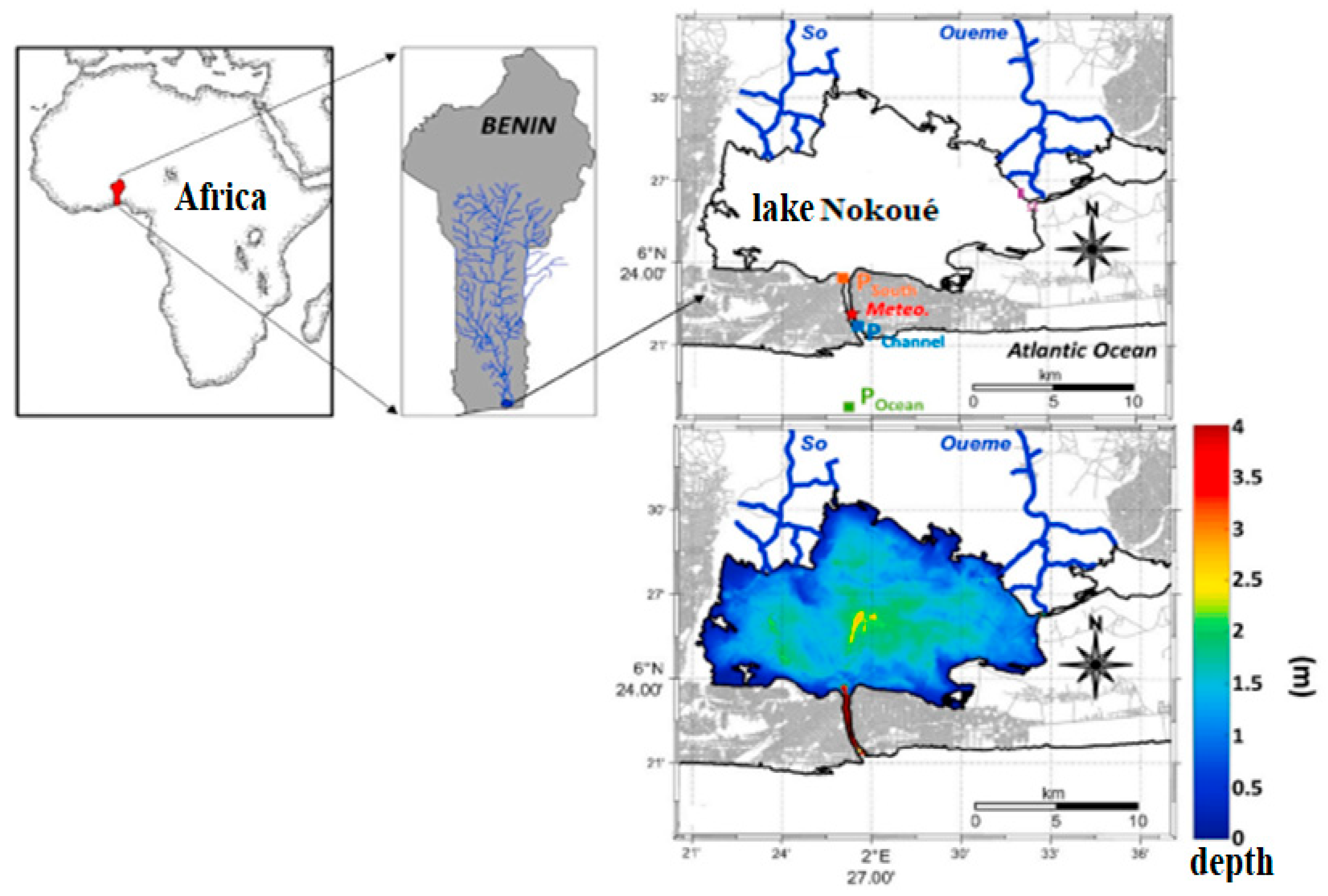
2.1. Study Areas

Nokoue lake is in southern Benin between a 6°38′ and 6°50′ north latitude, and a 2°35′ and 2°55′ west longitude. It varies between 150 and 170 km², respectively, during the low-water period and the high-water period (Figure 1).

2.2. Statistic Description of Water Level Peaks Values

This study focuses on the statistical analysis of the annual water level peaks of Nokoue lake, with data sourced from the Institute of Hydrology and Oceanology Research of Benin (IRHOB). An annual water level peak is defined as the maximum observed value within a year. These values were extracted from daily data collection covering the period from 1997 to 2022.

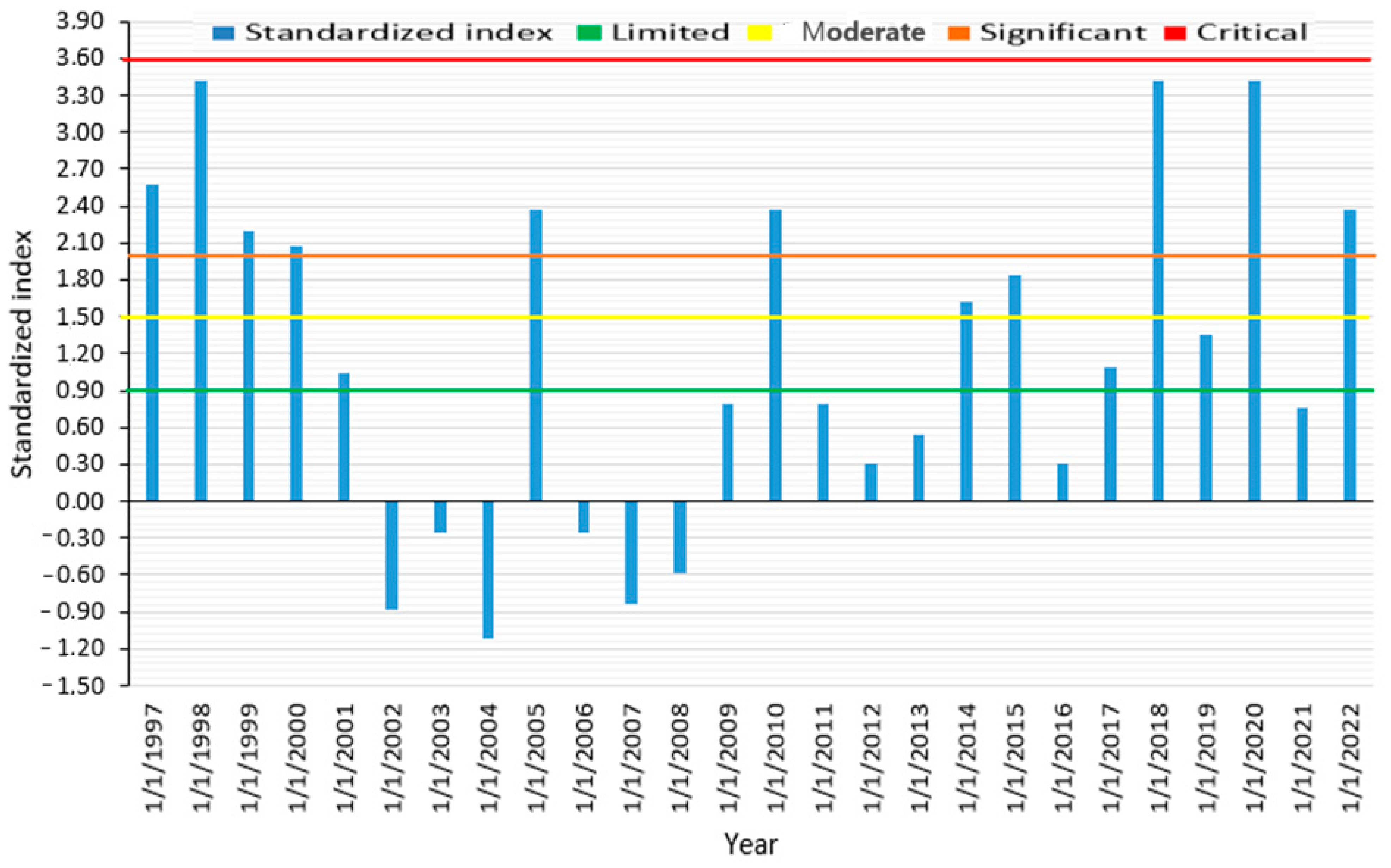
2.3. Standardized Water Level Peak Index Calculation and Categorization of Flood Hazards

The identification of flood hazard thresholds is based on three steps: the calculation of the standardized water level index, the representation of the standardized index based on annual water level peaks, and the projection of the normalized water level index on to the x-axis showing the annual water level peaks. The categorization of flood hazard alert thresholds for Nokoue lake is based on the standardized water level index inspired by McKee’s study. By normalizing the annual water level peak series of Nokoue lake, these thresholds were determined [23]. The formula for the water level index is as in Equation (1).

$$I_h={\displaystyle \frac{X_i-\overline{X}}{\sigma }}$$

(1)

where $I_h$ is the water level index, $X_i$ is the observed annual maximum value, $\overline{X}$ is the mean of the annual peak water level values, and $\sigma$ is the standard deviation of the annual water level peaks values. The different hazard categories, limited, moderate, significant, and critical, are shown in

Table 1. Categorization of flood hazard alert thresholds.

Risk Level	Hazard Categories
Critical	$I_h$ ≥ 2.0
Significant	1.5 ≤ $I_h$ < 2
Moderate	1 ≤ $I_h$ < 1.5
Limited	<1

.

2.4. Implementation of Frequency Models

Extreme water levels are estimated using a method of statistical fitting and extrapolation of extremes. Only the main points of the method are outlined here. For more information, please refer to [24]. The calculations were performed using the R environment because it is well known nowadays. The methodology for establishing frequency fitting curves consists of three main steps: (i) data selection, (ii) statistical tests (stationarity, independence, and homogeneity), (iii) the selection and calculation of the empirical probabilities of the extracted annual water level peak values, and fitting to estimate (iv) the parameters of the distribution and (v) the quantiles corresponding to several specified return periods associated with exceedance frequencies.

2.4.1. Selection of the Data

The extraction of extreme variables is a crucial step in statistical modeling. Indeed, the quality of the results depends primarily on the care taken during this step. The theory of extreme values has been developed by several authors [12,25,26,27,28,29]. There are several methods for extracting descriptive variables based on extreme value theory [30]. However, the method adopted in this study was the extraction of annual maximum values from the daily water height series for the period 1997–2022. This involved selecting, for each calendar year (from 1 January to 31 December), the highest daily water level, referred to as the annual maximum daily water height.

The statistical modeling of extreme values based on the extraction of annual maximum daily values is generally preferred over the method based on the extraction of extreme values exceeding an arbitrarily set threshold, both by researchers and practitioners. This preference is due to its superior statistical efficiency [30,31,32]. Several authors use the same variable—annual maximum daily flows or water heights—to model extreme water levels [33]. The technique of extracting values exceeding an arbitrarily set threshold is typically used when the length of the series is less than 10 years.

2.4.2. Statistic Hypothesis

The statistical methods generally used to verify stationarity, independence, and homogeneity are the Mann–Kendall, Wald–Wolfowitz, and Wilcoxon tests, respectively. These are robust statistical methods that are commonly employed [11]. These statistical tests follow a common principle: formulating a hypothesis regarding the sample of observations and then evaluating whether the observed data are consistent with the formulated hypothesis [34,35].

The hypothesis being tested, also referred to as the null hypothesis ($H_0$), is always accompanied by an alternative hypothesis ($H_1$). The acceptance or rejection of the null hypothesis is based on the probability value (p-value). The p-value represents the hazard of error in considering $H_0$—which assumes the sample is stationary, homogeneous, or independent [34,35].

In this study, the maximum acceptable p-value is set at 5%. In other words, a p-value greater than 0.05 indicates non-stationarity, non-independence, or non-homogeneity in the time series. Conversely, if the p-value is less than 5%, there is less than a one-in-twenty chance of error in concluding that the tested series of annual daily maximum water levels is not independent, stationary, or homogeneous. In simpler terms, the hazard of error is not statistically significant if the p-value is less than or equal to 5%.

✓

Stationarity test

A series of random variables is said to be stationary if its statistical characteristics (mean, variance, or moments) remain invariant over time [36]. The Mann–Kendall test was used to verify stationarity, allowing us to test the following hypotheses:

H0: 

The statistical characteristics of the random variables are constant over time.

H1: 

The statistical characteristics of the random variables are not constant over time.

Given $n$ random variables $x_1, x_2, x_3, \dots , x_n$arranged in chronological order, the test statistic $S$ is expressed as in Equation (2):

$$S={{\displaystyle \sum }}_{i=1}^{n-1}{{\displaystyle \sum }}_{j=i+1}^{n}sign\left(X_j-X_i\right)$$

(2)

Under $H_0$, the statistic $S$asymptotically follows a normal distribution with a mean of zero and a variance $var\left(S\right)$. The closer the test statistic $S$ is to zero, the more the observations are stationary.

✓

Independence test

A data series is said to be independent if one data point is not influenced by the preceding data point [37]. For the implementation of this test, we used the Wald–Wolfowitz test. It allowed us to verify the following hypotheses:

H0. 

The series is independent.

H1. 

The series is not independent.

When the series is sufficiently large, the Wald–Wolfowitz statistic $W$follows a normal distribution $U$with mean $\overline{w}$and variance $var\left(W\right)$ as shown in the Equation (3). Let $x_1, x_2, x_3, \dots , x_n$be random variables; then,

$$W={{\displaystyle \sum }}_{i=1}^{n-1}{x}_i\ast x_{i+1}+x_n\ast x_1$$

(3)

✓

Homogeneity test

A sample of a random variable is said to be homogeneous when its data points come from the same distribution (collected under the same conditions). Several statistical tests (Mann–Whitney test, Kruskal–Wallis test, Wilcoxon test, etc.) are used to ensure the homogeneity of a statistical series. The homogeneity test introduced by [38] was selected for this study. It is a non-parametric test that uses the ranks of observations instead of the actual values. Mathematically, the problem is formalized as follows: Given a series of observations of length $N$, from which two samples, $X$ and $Y$, are drawn, let $N_1$ and $N_2$ be the sizes of these samples, with $N=N_1+N_2$ and$N_1<N_2$. The values in the series are then ranked in ascending order. We then focus only on the rank of each element in the two samples within this series. If a value appears multiple times, it is assigned the corresponding average rank. Next, we calculate $W_x$ using Equation (4) [38]:

$$W_x={{\displaystyle \sum }}_{k=1}^{n1}rank\left(X\right)$$

(4)

2.4.3. Empirical Probability Calculation

The experimental probabilities associated with the observations were calculated using Weibull’s empirical formula, as shown in Equation (2), which aims to obtain unbiased exceedance probabilities for all distributions [39]. After ranking the sample of annual maximum daily water levels of size $N$ in ascending order, the expression for Weibull’s empirical or experimental exceedance frequency for a value $x_i$ of rank $i$ is given in Equation (5):

$$p\left(x_i\right)={\displaystyle \frac{i}{N+1}}etT\left(x_i\right)={\displaystyle \frac{1}{1-p\left(x_i\right)}}$$

(5)

where p is the exceedance probability of the annual water level peak, $i$ is the rank of the peak in the series, and $N$ is the size of the series consisting of the annual water level peaks.

2.4.4. Probability Distribution Functions

A parametric statistical distribution was fitted to the annual maximum daily water levels. Adopting a statistical distribution to study and describe water levels is undoubtedly the most critical step, introducing the greatest uncertainties [38,39]. It is important to test other distributions within the asymptotic domain of extreme events. Various approaches can help guide this choice, but unfortunately, no universal or foolproof method exists [40].

The first approach is based on local practices that, over time, have become true customs, even rules. Such choices often result from the experience of one or more authors, eventually forming schools of thought. The second approach involves theoretical considerations used to model the behavior of annual maxima. In this study, three distributions with relatively complementary behaviors were tested [41,42]: the Generalized Extreme Value (GEV) distribution, the Gumbel distribution, and the Generalized Pareto (GPA) distribution. These belong to the family of generalized extreme distributions and are often used to model extreme events, such as river or lake floods.

A comparative performance study of the recommended distributions, as proposed by [38,39,40], is the most suitable way to justify the choice of a distribution. The method of L-moments, based on the negative log-likelihood, was used to estimate the parameters of the statistical distributions [43]. The distribution functions of the three laws used in this study are presented in equations 6 to 8.

• The probability density function of the Gumbel distribution [41]:

$$f\left(x\right)={\displaystyle \frac{1}{\alpha }}{e}^{-\left({\displaystyle \frac{x-\mu }{\alpha }}\right)}{e}^{-e^{-\left({\displaystyle \frac{x-\mu }{\alpha }}\right)}}$$

(6)

where $\alpha$ is the scale parameter and $\mu$ is the location parameter.

• The probability density function of the GEV [42]:

$$f\left(x\right)={\displaystyle \frac{1}{\alpha }}{\left(1+{\displaystyle \frac{k\left(x-\mu \right)}{\alpha }}\right)}^{-{\displaystyle \frac{-1}{k}}-1}\times e^{\left(-{\left(1+{\displaystyle \frac{k\left(x-\mu \right)}{\alpha }}\right)}^{-{\displaystyle \frac{1}{k}}}\right)}$$

(7)

where $k$ is a positive, non-zero shape parameter; $\mu$ is a location parameter; and $\alpha$ is a scale parameter.

In the case where $k=0$, this distribution simplifies to the Gumbel distribution.

• The probability density function of the GPA [43]:

  $$f\left(x\right)={\displaystyle \frac{1}{\alpha }}{\left(1+{\displaystyle \frac{k\left(x-\mu \right)}{\alpha }}\right)}^{-{\displaystyle \frac{1}{k}}-1}$$

  (8)

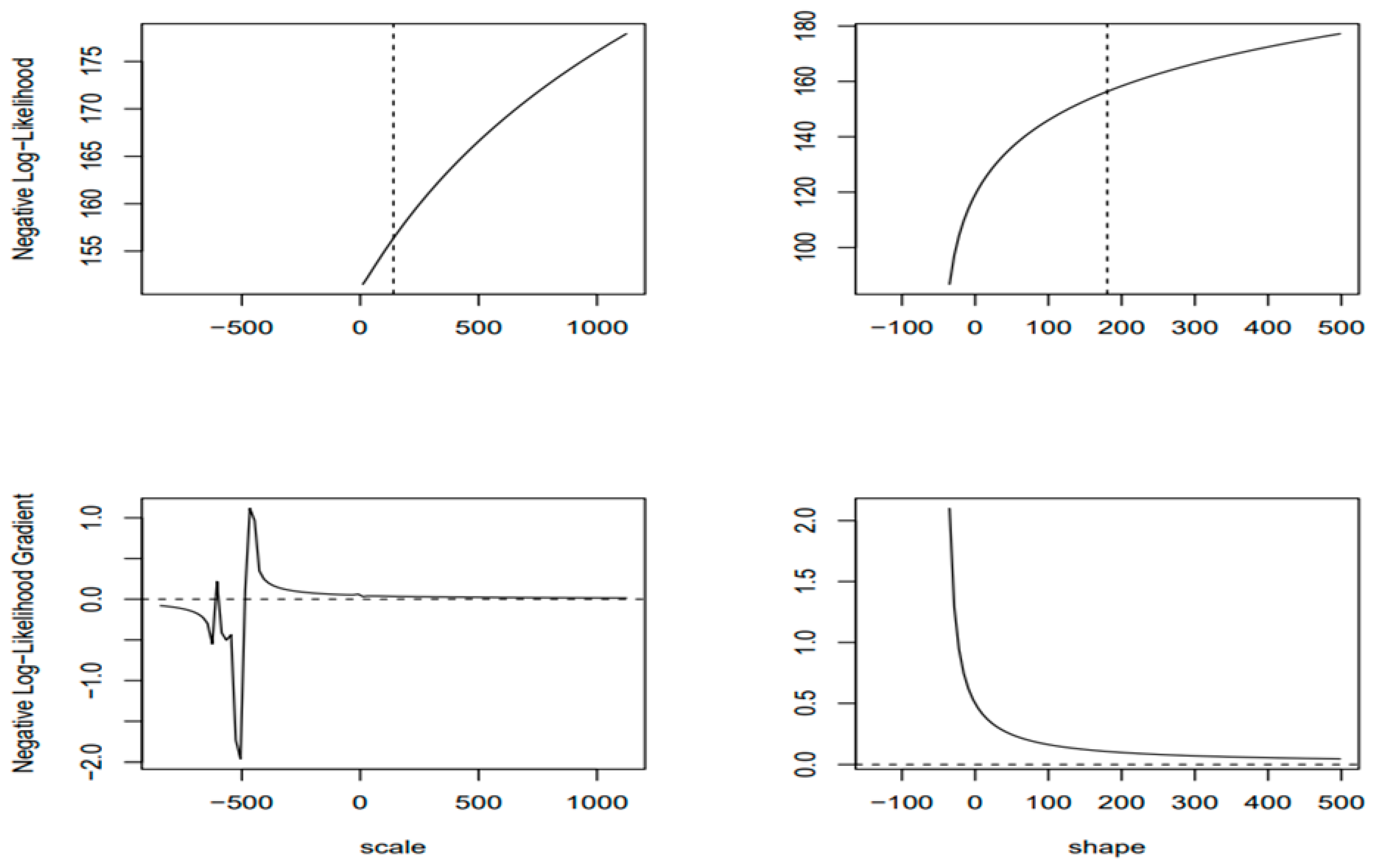
2.4.5. Estimation of Parameters

The linear moments used to estimate the parameters of the distribution in this study are linear combinations of weighted probability moments. The estimators are derived from solving a system of equations that equates the sample linear moments with those of the theoretical distribution to be fitted. For the linear moment method [44], which proposes numerous distributions ranging from 1 to 5 parameters, the method is formalized as follows:

Let $x$ be a random variable with distribution function $F$, and let $x_{1:n}$, $x_{2:n}$, $x_{3:n}$, …, $x_{n:n}$ represent the order statistics for a sample of size $n$. The order statistics $1,2,3,\dots n$ for a sample of size $n$ are given in Equation (9) [44]:

$${\lambda }_r=r^{-1}{{\displaystyle \sum }}_{k=0}^{r-1}{\left(-1\right)}^k\left(\begin{array}{c}r-1\\ k\end{array}\right)E\left(x_{r-k:r}\right)$$

(9)

with $\left\{\begin{array}{c}r=1,2,3,\dots n\\ E\left(x_{j:r}\right)={\displaystyle \frac{r!}{\left(j-1\right)!\left(r-j\right)!}}\int {\left\{x\left(f\left(x\right)\right)\right\}}^{j-1}\ast \left\{{\left(1-F\left(x\right)\right)}^{r-1}\right\}dF\left(x\right)\end{array}\right.$, where $E$ represents the mean of the random variable $x$, $\lambda$ represents the moment, and $r$ represents the order of moments.

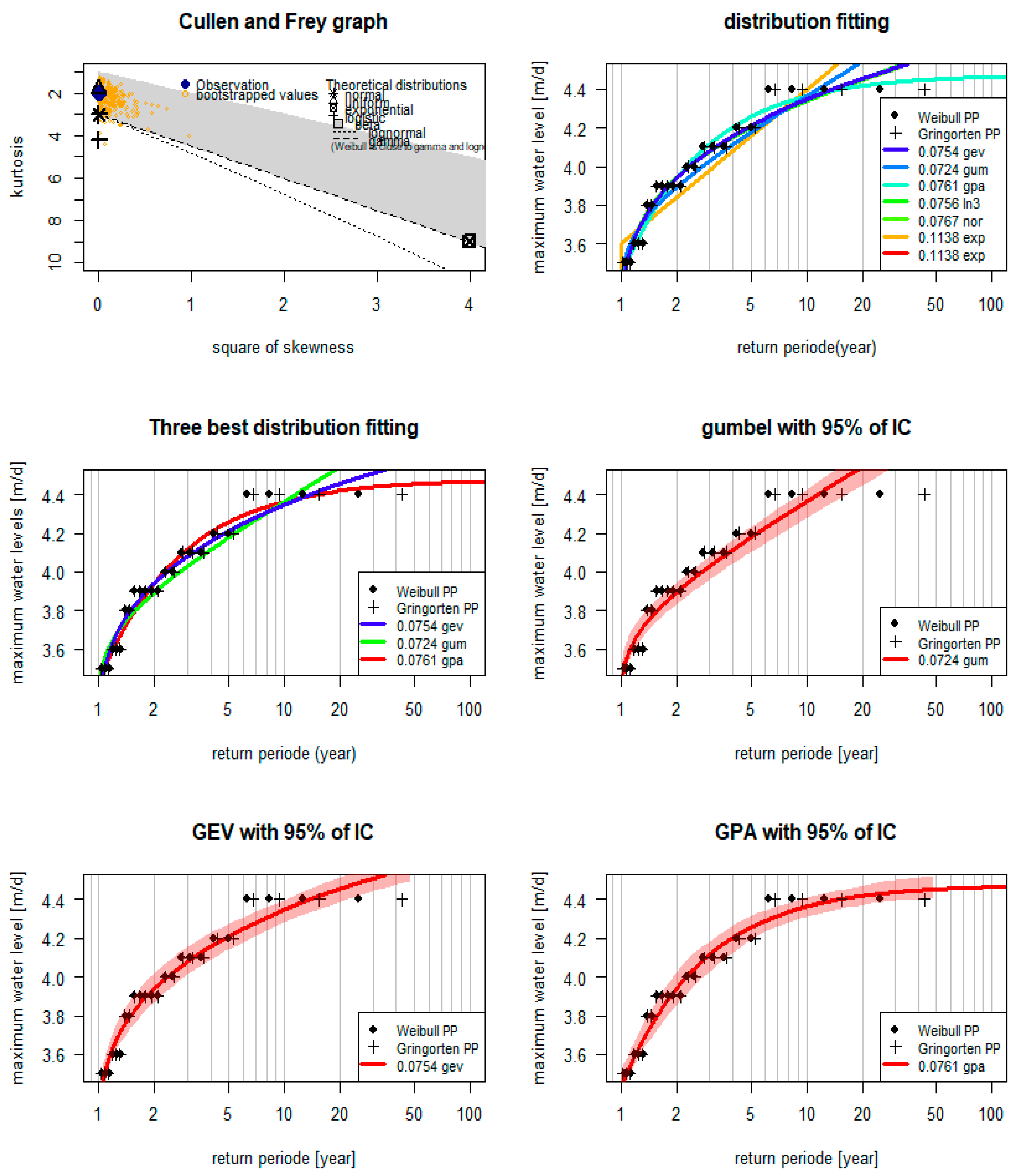
2.4.6. Goodness-of-Fit Test to Identify the Best-Fitting Distribution

The quality of the statistical extrapolation of extreme events is assessed using linear moments diagrams, Taylor diagrams, cumulative distribution functions, and the root-mean-square error (RMSE). They are the most frequently used goodness-of-fit tests [44].

• Root-mean-square error criterion

The root-mean-square error (RMSE) is a method for objectively evaluating the performance of models. It provides a measure of the average magnitude of prediction errors, with lower values indicating better model accuracy. It is formulated as follows in Equation (10) [45]:

$$RMSE=\sqrt{{\displaystyle \frac{1}{N}}{{\displaystyle \sum }}_{i=1}^N(O_n-M_n}{)}^2$$

(10)

where $O_n$ is the observed values and $M_n$ is the predicted values.

• Linear moments diagram

The linear moments diagram is based on the combination of skewness coefficients (${\tau }_3$) and kurtosis coefficients (${\tau }_4$) to graphically assess which distribution best fits the sample observations. Constructing the diagram requires knowledge of the function relating ${\tau }_3$ to ${\tau }_4$ through the formula in Equation (11) [46]:

$$\tau 4={{\displaystyle \sum }}_{j=0}^8{a}_j({\tau }_3^2)$$

(11)

where a_j is the polynomial approximation coefficient.

• Taylor diagram

It is a three-dimensional diagram that visualizes the relationship between observed and simulated data using three concise statistical parameters: the coefficient of determination $\left(R^2\right)$, the root-mean-square error $\left(RMSE\right)$, and the standard deviation ($\sigma$). To create this, we used the plotrix package with its Taylor diagram function in R, which evaluates both the correlation and the RMSE between the empirical and theoretical distributions. Let $O_n$ and $M_n$ be the observed values and model predictions with respective means and standard deviations, ${\mu }_1, {\sigma }_1$ and ${\mu }_2, {\sigma }_2$, where $n=1,2,3,\dots ,N$and $N$ is the number of observations. The statistical parameter $R^2$ is given by Equation (12) [47]:

$$R^2=1-{\displaystyle \frac{{{\displaystyle \sum }}_{i=1}^n{\left(Q_{obs}^i-Q_{sim}^i\right)}^2}{{{\displaystyle \sum }}_{i=1}^n{\left(Q_{obs}^i-{\overline{Q}}_{obs}\right)}^2}}$$

(12)

where $Q_{obs}^i$ represents the observed values and $Q_{sim}^i$ represents the simulated values.

2.4.7. Application to Pre-Determination

The comparative analysis of quantiles is based on the principle that the concept of hydrological norms assumes climate stability [16]. The statistical distribution selected based on its performance was used to pre-determine the floods of Nokoue lake. The actual application involved using the statistical distribution to determine the value of a quantile ${\mathit{X}}_{\mathit{q}}$ based on a cumulative frequency or, conversely, to calculate the return period corresponding to a given quantile value ${\mathit{X}}_{\mathit{q}}$ [46]. After estimating the different quantiles, the calculation of confidence intervals was performed to define a range of variation for the estimates according to the confidence level set. The confidence interval represents “the space of ambiguity, imprecision, and mismatch of a reality that resists being bound by a formula governing its distribution”. To define it, a certain hazard α of being wrong must be accepted [28]. To achieve this, the non-parametric bootstrap test was used with a 95% confidence interval to define the limits of the estimated quantiles [44]. The quantiles of the maximum daily water level of Nokoue lake were evaluated for several non-exhaustive return periods (2, 5, 10, 20, 50, and 100 years) based on the three best-performing distributions. In hydraulic design projects, the choice of return period depends on the importance of the hydraulic structure to be designed [1,46]. However, some typical return periods used in the design of flood hazard management and drainage works include the following [46]:

• Two to five years for primary to tertiary channels.
• Ten years for small crossing structures such as pipes and culverts.
• Twenty to fifty years for small to medium-sized bridges.
• One hundred years for major bridges (greater than 100 m in span).

3. Results

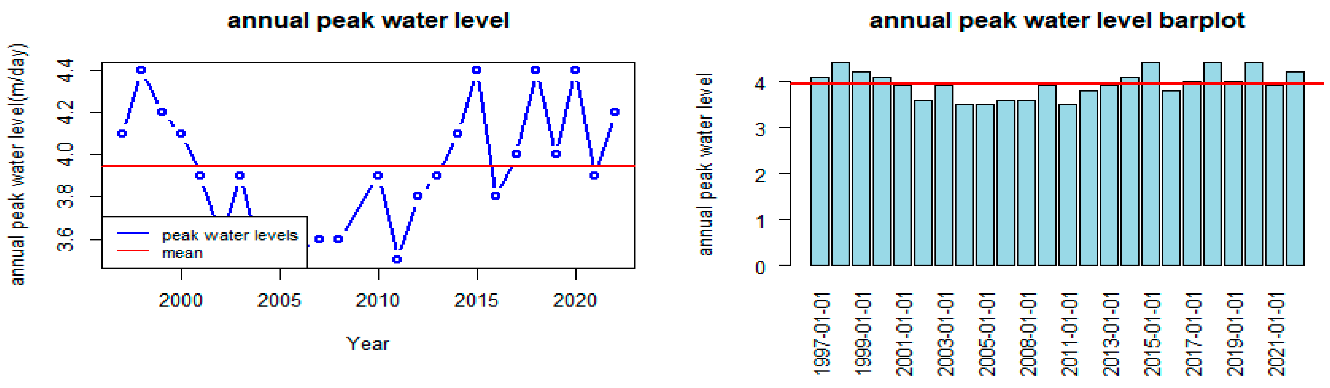
3.1. Description of the Annual Water Level Peaks Values

The statistical examination of the data series indicated that, over a 27-year period, the water level peaks of Nokoue lake ranged from 3.5 to 4.4 m, observed in 1997 and 2022, respectively, with 3.95 m as the mean annual water level peak of Nokoue lake (

Table 2. Summary statistics of annual peak water level values.

Min	25%	50%	75%	Max	Standard Deviation
3.5	3.75	3.95	4.13	4.4	0.2

, Figure 2).

3.2. Results of Standardized Water Level Index

Figure 3 shows the different categories flood hazard based on the standardized water level peak index and the interannual evolution of the annual water level peak index in the Nokoue lake watershed. The analysis of Figure 3 reveals that the water level peak index for Nokoue lake exhibits variability throughout the entire series. Additionally, a positive index characterizes wet years, ranging from 0.3 to 3.3 in the Nokoue lake watershed. Eight years are considered extremely wet across the watershed based on a standardized water level index that exceeds +2. Similarly, three hydrological phases emerge from the examination of Figure 3. The first phase corresponds to the period 1997–2001, characterized by a high frequency of positive indices; among the eight extremely wet years, three (1997, 1998, and 1999) fall within this phase. The second phase spans from 2002 to 2008, marked by a decline in annual peak water levels and a predominance of negative indices (not covered in this study). The final phase covers the period from 2009 to 2022, characterized by a slight recovery in peak water level with a positive index. This resurgence in water level peaks is due to extreme rainfall events, which can cause floods and socioeconomic and environmental damage within the study area. This was the case in 2018, 2020, and 2022, during which the Nokoue lake watershed recorded a positive index of +3.3.

Figure 4 shows the identified alert thresholds for water levels in the Nokoue lake watershed.

The analysis of Figure 4 indicates that the water level threshold classes are as follows: limited hazards up to 3.94 m, moderate hazards between 3.94 and 4.04 m, significant hazards between 4.04 and 4.14 m, critical hazards between 4.14 and 4.95 m. At the moderate hazard threshold, flooding may occur if the watershed receives a certain amount of rainfall, with the extent of flooding being moderate. The significant and critical hazard thresholds are more prominent in the Nokoue lake watershed, helping to characterize hydrologically wet years when flood events are predominant as the watershed experiences rainfall. This is not without socioeconomic and ecological consequences in the study area.

3.3. Results of Hypothesis Tests

The results of statistical tests conducted on the extracted annual peak water level data indicate a rejection of the alternative hypothesis ($H_1$) in each test (

Table 3. Results of the statistical tests.

Statistical Tests	p-Value	Status
Independance	0.12	accepted
Homogeneity	0.14	accepted
Stationarity	0.14	accepted

). Given that if the p-value is greater than 0.05, the null hypothesis ($H_0$) is accepted, this outcome implies homogeneity, independence, and stationarity among the annual peak water levels.

• The hypothesis that the data series of annual peak water levels is independent is accepted with a 95% confidence level. There is no correlation between the data in the series.
• The absolute value of the Mann–Kendall statistic $\left(\left|K\right|\right)$ is evaluated at 0.14. The hypothesis that there is no trend in data series is accepted at a 5% significance level.
• The absolute value of the Wilcoxon statistic $\left(\left|W\right|\right)$ is evaluated at 0.14. The mean of the two sub-samples (1997–2015 and 2016–2022) is statistically equal, meaning the series is homogeneous. Thus, the null hypothesis $H_{0 }$is accepted at a 5% significance level.

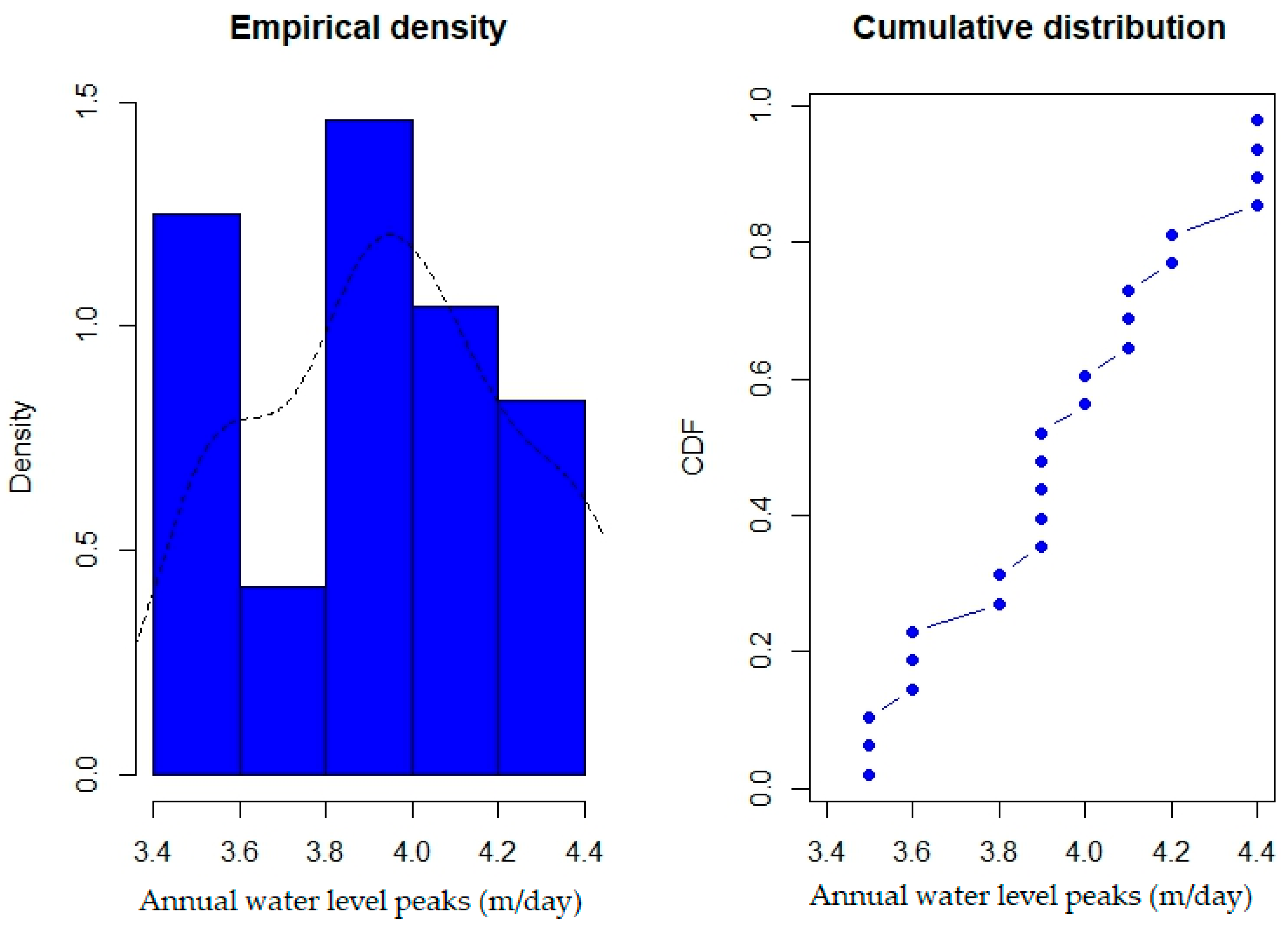
3.4. Results of Empirical Probability

The empirical probability density is composed of two phases: a rising phase from 0.3 to 1.2 and a declining phase from 1.25 to 0.5. The highest empirical probability densities are between 3.8 m and 4.0 m (Figure 5).

3.5. Results of Fitting to Statistical Distributions

The L-moment estimation method applied to determine the parameters of the three best distributions, Gumbel, GEV, and GPA, fitted to the annual peak water level of Nokoue lake yielded the following results (

Table 4. The results of the parameters for the Gumbel, GEV, and GPA distributions.

Statistical Distributions	Parameters
	$\mathit{\mu }$	$\mathit{\alpha }$	$\mathit{k}$
Distribution of Gumbel	3.80	0.25
Distribution of GEV	0.30	0.3	0.27
Distribution of GPA	3.43	1.003	0.96

, Figure 6, Figure 7, Figure 8 and Figure 9).

The Cullen and Frey graph (Figure 9) compares the data to theoretical distributions and guides the selection of the appropriate statistical model. Here, the fit seems to indicate that the data follow an asymmetric distribution with moderate kurtosis. This suggests heavy-tailed distributions such as the Gumbel, GEV, and GPA distributions, as well as the Gamma and Weibull distributions. The plots of the annual peak water level of Nokoue lake as a function of return period, created on a semi-logarithmic scale, do not perfectly follow the shapes of the various distribution curves. Figure 9 below shows the results of the fitting performed for each of the three best statistical distributions, Gumbel, GEV, and GPA. According to Figure 9, the “Three Best Fits of the Distribution” plot, the graphical analysis indicates that the scatterplot is best represented by the Gumbel distribution. The result of the root-mean-square error (RMSE) of the Gumbel distribution is estimated to be 0.0724 (Figure 9). It is the smallest value of the observed root-mean-square error, indicating that the Gumbel distribution best represents the annual peak water level of Nokoue lake. It is important to note that the performance evaluation focused on the ability of different theoretical distributions to replicate the sample of peak water level values for Nokoue lake. For this purpose, cumulative distribution function curves, L-moment diagrams, and Taylor diagrams were constructed to identify the best-fitting distributions. The comparison of the cumulative distribution function of the Gumbel distribution with those of the GEV and GPA distributions fitted to the annual peak water level revealed different root-mean-square errors (RMSE). The Gumbel distribution performed best, with an RMSE of 0.0724, compared to RMSEs of 0.0754 for the GEV distribution and 0.0761 for the GPA distribution, respectively (Figure 10a, 10b). Recall that the L-moment diagram is a graphical representation of the coefficients of kurtosis against the coefficients of skewness. These were plotted to compare the distributions that align with the sample of the annual peak water level for Nokoue lake. This representation showed that the L-moment diagrams of both the Gumbel and GEV distributions closely approximate the annual peak water levels of Nokoue lake (Figure 10d). The Taylor diagram was used to evaluate the root-mean-square error (RMSE), correlation coefficient, and standard deviation for the Generalized Extreme Value (GEV) distribution applied to the sample of the annual peak water level of Nokoue lake. The comparison of these coefficients revealed that the Gumbel model has the highest correlation coefficient, estimated to be 97%, and the lowest values of the RMSE and standard deviation ($\sigma$), estimated to be 0.45 and 1, respectively (Figure 10c).

3.6. The Results of the Water Level Peak Estimates for the Gumbel, GEV, and GPA Distributions

For the preliminary determination of flood quantiles at extreme frequencies and the return period (RP) of the reference flood, the three best distributions were selected based on their superior performance in the model selection tests (

Table 5. The exceedance probability associated with the estimated quantiles and the RMSE of the distributions.

	0.85	0.75	0.5	0.25	0.2	0.1	0.01	RMSE
Gumbel	3.642573	3.720708	3.893353	4.112385	4.175660	4.362572	4.947841	0.07238795
GEV	3.625181	3.732998	3.941547	4.156290	4.209517	4.347250	4.636763	0.07543231
GPA	3.585419	3.686597	3.941998	4.202556	4.255658	4.363591	4.465037	0.07610624
Empirical	3.598333	3.683333	3.900000	4.158333	4.200000	4.400000	4.400000
Quantile mean	3.592593	3.663426	3.900000	4.134954	4.200000	4.400000	4.400000

and

Table 6. Quantile values associated with return periods.

	RP.2	RP.3	RP.6	RP.7	RP.8	RP.9	RP.10
Gumbel	3.893353	4.026908	4.225984	4.267789	4.303554	4.334811	4.362572
GEV	3.941547	4.078418	4.249350	4.280847	4.306698	4.328494	4.347250
GPA	3.941998	4.114921	4.291336	4.316985	4.336328	4.351446	4.363591
Empirical	3.500000	3.900000	4.200000	4.322222	4.400000	4.400000	4.400000
Q mean	3.500000	3.900000	4.200000	4.270988	4.384127	4.400000	4.400000
	RP.15	RP.20	RP.30	RP.35	RP.40	RP.45	RP.50
Gumbel	4.468026	4.541862	4.645004	4.684007	4.717721	4.747411	4.773935
GEV	4.413629	4.455843	4.509497	4.528292	4.543918	4.557220	4.568751
GPA	4.400367	4.419004	4.437885	4.443340	4.447454	4.450669	4.453252
Empirical	4.400000	4.400000	4.400000	4.400000	4.400000	4.400000	4.400000
Q mean	4.400000	4.400000	4.400000	4.400000	4.400000	4.400000	4.400000
	RP.55	RP.60	RP.70	RP.75	RP.80	RP.85	RP.90
Gumbel	4.797905	4.819768	4.858464	4.875768	4.891948	4.907140	4.921459
GEV	4.578894	4.587922	4.603390	4.610103	4.616268	4.621961	4.627242
GPA	4.455374	4.457148	4.459948	4.461073	4.462060	4.462933	4.463711
Empirical	4.400000	4.400000	4.400000	4.400000	4.400000	4.400000	4.400000
Q mean	4.400000	4.400000	4.400000	4.400000	4.400000	4.400000	4.400000
	RP.95	RP.100
Gumbel	4.934999	4.947841
GEV	4.632162	4.636763
GPA	4.464408	4.465037
Empirical	4.400000	4.400000
Q mean	4.400000	4.400000

). The Gumbel distribution appears to fit the tail of the distribution better. For exceedance probabilities ranging from 0.85 to 0.01, the quantiles estimated with the Gumbel distribution closely approximate the empirical quantiles (Table 5). The quantiles associated with return periods (RP) of 2, 3, 5, 6, 7, 8, 9, 10, 15, 20, 25, 30, 35, 40, 45, 50, 55, 60, 65, 70, 75, 80, 85, 90, 95, and 100 years are provided in Table 6. The reference flood for the Nokoue lake station is the highest recorded quantile value, corresponding to 5.05 m/day with the Gumbel distribution, with an associated return period of 150 years. This implies that the reference flood has a 0.66% chance of occurring or being exceeded annually. The annual peak water level for the 100-year return period is 4.95 m/day. The box plot (Figure 11) shows that most of the annual peak water levels of Nokoue lake estimated with the Gumbel distribution are below the mean.

4. Discussion

This study is a first for the Nokoue lake basin, highlighting the flood risk alert thresholds as well as the statistical distributions capable of reproducing the exceedance probabilities of the maximum daily water level of Nokoue lake using appropriate hydrological information. The standardized water level indexes for Nokoue lake, ranging from $-1.5$ to $+3.9$, allow for the categorization of hydrological thresholds, corresponding to the limited, moderate, significant, and critical hazard classes. This categorization of hydrological thresholds based on the standardized index or flood index helps define the extent of flooding in the Nokoue lake watershed. The evaluation of the standardized index of the maximum annual water level of Nokoue lake allowed for the categorization of the hydrological flood hazard thresholds of Nokoue lake into limited, moderate, significant, and critical hazard thresholds, thereby enhancing our predictive capacity regarding flood hazards in the Nokoue lake watershed. The analysis of the standardized index of the water level of Nokoue lake revealed light flooding 46.15% of the time, moderate flooding 11.54% of the time, severe flooding 7.69% of the time, and extreme flooding 34.62% of the time. According to [2,48,49], these hydrological flood hazard thresholds are strongly influenced by factors such as intense precipitation, soil moisture, and geomorphological properties (catchment size, topography). This categorization of hydrological thresholds helps define the extent of flooding in the Nokoue lake watershed. The magnitude or extent of flooding varies according to the level of hazard, as shown in Figure 3. The analysis of Figure 3 indicates that the periods 1997–2001 and 2009–2022 are characterized by a high frequency of positive indices in the Nokoue lake watershed, which could be explained by the fact that the study area experienced hydrologically wet periods, marked by probable flooding during these years [6]. The inflows from the Nokoue lake tributaries combined with excessive rainfall would be the cause. This return to a wet state aligns with previous studies conducted in West Africa, notably in Benin [50] and Nigeria [4] as well as elsewhere [51,52,53,54]. The three best statistical distributions show a concave shape with indefinite growth. This concavity is dictated by the sign of the shape parameter, which influences the curvature in the tails of the statistical distributions. Beyond the 10-year return period, the Gumbel distribution shows a more pronounced concavity compared to the GEV and GPA distributions. From an asymptotic perspective, the Gumbel distribution has proven to be the best fit for the sample of the maximum annual daily water level of Nokoue lake, making it the selected model. This can be explained by its asymptotic behavior [55] and because the Gumbel distribution provides acceptable results when the method of linear moments is used to estimate the parameters [5,56]. The Fisher–Tippett–Gnedenko theorem, based on extreme value theory, states that for a series of independent and identically distributed observations following a common distribution F, the limit of their linearly normalized maxima, as $N$ approaches infinity, converges to a Gumbel distribution [57,58,59,60,61]. Panthou [1], studying about thirty rainfall stations in West Africa, also demonstrated that the Gumbel distribution was well suited for determining extreme rainfall in 95% of catchments when the method of maximum annual daily rainfall is used. The statistical analysis of the quantiles from the probabilistic flood risk estimates of Nokoue lake, using the three best statistical distributions, Gumbel, GEV, and GPA, showed an upward trend in the exceedance probabilities of the most probable events for Nokoue lake. The work in [62] supported the idea that this trend may be due to the possible impact of climate change phenomena. For low exceedance probabilities, the Gumbel distribution tends to underestimate the quantiles compared to the GEV and GPA distributions. However, for high exceedance probabilities, it tends to overestimate the quantiles. This could be explained by the positive skewness coefficient of the series of maximum annual daily water heights. A positive skewness coefficient indicates that the values of daily water heights are dispersed to the right of the mean [63]. For medium exceedance probabilities, the three best distributions exhibit almost identical behavior. These results align with the studies in [57,58,59,60], which also used linear moment diagrams to conclude that the Gumbel and GEV distributions are reasonable representations of the annual maxima in homogeneous regions of the United States. According to [63], when the skewness coefficient of the series of annual maxima, which characterizes flash floods, is positive, asymmetric distributions (heavy tails) like Gumbel and GEV fit better than GPA. While we have not proven a causal link, flood regimes generally correspond to the statistical properties of the Gumbel and GEV distributions, as shown by the lines of the probability density functions and those of linear moments (Figure 9 and Figure 10). There are many examples where the Gumbel distribution gives remarkable results, but it seems that, under the same theoretical justifications, there may be interest in using the Fréchet distribution in some cases, especially due to its slower decay [61,62] demonstrated on a series of truncated values (values exceeding a fixed threshold) and using the robust linear moment method for estimating distribution parameters; the family of distributions that best describes peak flows evolves from the GPA distribution to Gumbel and then to the GEV distribution and the Log Normal type 3 (LN3) distribution. They confirmed that the tail of the GPA distribution is thicker as the value of the shape parameter k increases. Our results align with those of [58,59,60,61], who also demonstrated that the high variance in the ratios of linear moments (Figure 10d) could not solely be attributed to sampling errors. They observed a shift from the optimal Gumbel distribution to GEV with a decrease in total annual rainfall. They confirmed that using the linear moment method to estimate the parameters of extreme value distributions like Gumbel, GEV, and GPA is very effective and precise, using a global optimization tool that can avoid various local optima compared to the maximum likelihood method. It follows that quantiles can be accepted for the design of hydraulic structures in general, and flood control or drainage works in particular, in the Nokoue lake basin in Benin. For better safety of hydraulic flood evacuation works, this study recommends using quantiles from the Gumbel distribution for return periods of less than 50 years. For rare maximum annual daily water heights (50 and 100 years), it is possible to use the reference quantiles, along with those associated with a 150-year return period.

5. Conclusions

The Gumbel model correctly reproduces the curves of peak flood water levels for Nokoue lake. The return period of the largest flood experienced by Nokoue lake is 150 years. The Gumbel model will be used for the preliminary determination of the peak water level related to floods in the Nokoue lake watershed. The main limitation of this work lies in the choice of probability distributions and the method of parameter estimation. Indeed, there is no universal and infallible method for choosing the distributions suited to different situations. However, this case study of the Nokoue lake watershed serves as a basis for all flood prevention structures in the Nokoue lake watershed and the determination of alert thresholds.

References

1. Panthou, G. Analyse des Extrêmes Pluviométriques en Afrique de l’Ouest et de Leurs Evolution au Cours des 60 Dernières Années; Université de Grenoble: Saint-Martin-d’Hères, France, 2013. [Google Scholar]
2. Domiho, J.K. Indicateurs des évènements Hydroclimatiques Extrêmes dans le Bassin Versant de l’Ouémé à l’exutoire de Bonou en Afrique de l’Ouest. Ph.D. Thesis, Université Montpellier, Montpellier, France, 2018. [Google Scholar]
3. Chaigneau, A. From seasonal flood pulse to seiche: Multi-frequency water-level fluctuations in a large shallow tropical lagoon (Nokoué Lagoon, Benin). Estuar. Coast. Shelf Sci. 2022, 267, 107767. [Google Scholar] [CrossRef]
4. Yonaba, R.O. Dynamique Spatio-Temporelle des états de Surface et Influence sur le Ruissellement sur un Bassin de Type Sahélien: Cas du Bassin de Tougou (Nord Burkina Faso). Ph.D. Thesis, Institut International d’Ingénierie de l’Eau et de l’Environnement, Ouagadougou, Burkina Faso, 2020. [Google Scholar]
5. Descroix, L.; Diongue, A.N.; Dacosta, H.; Panthou, G.; Quantin, G.; Diedhiou, A. Évolution des pluies de cumul élevé et recrudescence des crues depuis 1951 dans le bassin du Niger moyen (Sahel). Climatologie 2013, 10, 37–49. [Google Scholar] [CrossRef]
6. Ogunrinde, A.T.; Oguntunde, P.G.; Akinwumiju, A.S.; Fasinmirin, J.T. Analysis of recent changes in rainfall and drought indices in Nigeria, 1981–2015. Hydrol. Sci. J. 2019, 64, 1755–1768. [Google Scholar] [CrossRef]
7. Daouda, M. Caractérisation d’un Système Lagunaire en Zone Tropicale: Cas du lac Nokoué (Bénin). Eur. J. Sci. Res. 2011, 56, 516–528. [Google Scholar]
8. Kawoun, A.G.; Bernard, A.; Chabi, A.; Ayena, A.; Adandedji, F.; Vissin, E. Variabilité Pluvio-Hydrologique et Incidences sur les Eaux de Surface dans la Basse Vallée de l’Ouémé au Sud-Est Bénin. Int. J. Progress. Sci. Technol. (IJPSAT) 2020, 23, 52–65. [Google Scholar]
9. Hounvou, S.F.; Guedje, F.K.; Kougbeagbede, H.; Adechinan, J.; Houngninou, E. Analyse statistique des pluies journalières extrêmes à partir d’un seuil dans le Bénin subéquatorial. J. Phys. SOAPHYS 2019, 1, 1–6. [Google Scholar] [CrossRef]
10. GIEC. Sixième Rapport d’évaluation du GIEC: Changement Climatique 2022|UNEP—UN Environment Programme. 2022. Available online: https://www.unep.org/fr/resources/rapport/sixieme-rapport-devaluation-du-giec-changement-climatique-2022 (accessed on 22 October 2024).
11. Kouassi, A.M.; Nassa, R.A.-K.; Yao, K.B.; Kouame, K.F.; Biemi, J. Modélisation statistique des pluies maximales annuelles dans le district d’Abidjan (sud de la Côte d’Ivoire). Rev. Des Sci. L’eau 2018, 31, 147–160. [Google Scholar] [CrossRef]
12. Kouassi, A.M.; Nassa, R.A.-K.; Kouakou, K.E.; Kouame, K.F.; Biemi, J. Analyse des impacts des changements climatiques sur les normes hydrologiques en Afrique de l’Ouest: Cas du district d’Abidjan (sud de la Côte d’Ivoire). Rev. Sci. L’eau 2020, 32, 207–220. [Google Scholar] [CrossRef]
13. Hounkpè, J.; Diekkrüger, B.; Badou, D.F.; Afouda, A.A. Non-stationary flood frequency analysis in the Ouémé River Basin, Benin Republic. Hydrology 2015, 2, 210–229. [Google Scholar] [CrossRef]
14. Dèhoué, P. Gestion des risques d’inondation dans le bassin versant du lac Nokoué. Water Resour. Manag. 2021. [Google Scholar] [CrossRef]
15. Akodjinou, J. Analyse des vulnérabilités climatiques dans le bassin du lac Nokoué. Clim. Change 2022. [Google Scholar] [CrossRef]
16. Alassane, A. Analyse hydrologique des crues dans le bassin versant du lac Nokoué. Hydrol. Earth Syst. Sci. 2020. [Google Scholar] [CrossRef]
17. Yue, S.; Pilon, P. A Comparison of the power of the test, Mann–Kendall and bootstrap tests for trend detection. Hydrol. Sci. J. 2004, 49, 21–38. [Google Scholar] [CrossRef]
18. Lamarre, H. Musy, André et Higy Christophe. In Hydrologie, une Science de la Nature; Coll. Gérer l’environnement; Presses Polytechniques et Universitaires Romandes: Lausanne, Switzerland, 2004; 314p. [Google Scholar]
19. Dabire, N.; Ezin, E.C.; Firmin, A.M. Forecasting Nokoue lagon Water Levels Using Long Short-Term Memory Network. Hydrol. J. 2024, 11, 161. [Google Scholar] [CrossRef]
20. Namwinwelbere, D.; Eugène, E.C.; Firmin, A.M. Current State of Flooding and Water Quality of Nokoue Lake in Benin (Ouest Africa). Eur. J. Environ. Earth Sci. 2022, 3, 75–81. [Google Scholar] [CrossRef]
21. Dabire, N.; Ezin, E.C.; Firmin, A.M. Water quality index of nokoue lagon prediction using random forest and artificial neural network. Int. J. Adv. Res. 2024, 12, 610–624. [Google Scholar] [CrossRef]
22. Dabire, N.; Ezin, E.C.; Firmin, A.M. Water Quality Assessment Using Normalized Difference Index by Applying Remote Sensing Techniques: Case of Nokoue lagon. In Proceedings of the 2024 IEEE 15th Control and System Graduate Research Colloquium (ICSGRC), Shah Alam, Malaysia, 17 August 2024; p. 6. [Google Scholar]
23. Ali, A.; Lebel, T. The Sahelian standardized rainfall index revisited. Int. J. Climatol. 2009, 29, 1705–1714. [Google Scholar] [CrossRef]
24. Guerreiro, M. Flood Analysis with the Standardized Precipitation Index (SPI); Edições Universidade Fernando Pessoa: Porto, Portugal, 2008. [Google Scholar]
25. Karim, F.; Hasan, M.; Marvanek, S. Evaluating annual maximum and partial duration series for estimating frequency of small magnitude floods. Water 2017, 9, 481. [Google Scholar] [CrossRef]
26. Marani, M.; Ignaccolo, M. A metastatistical approach to rainfall extremes. Adv. Water Resour. 2015, 79, 121–126. [Google Scholar] [CrossRef]
27. Pappenberger, F. The extreme runoff index for flood early warning in Europe. Nat. Hazards Earth Syst. Sci. Discuss. 2023, 14, 1505–1515. [Google Scholar]
28. Tie, A.G.B.; Konan, B.; Brou, Y.T.; Issiaka, S.; Fadika, V.; Srohourou, B. Estimation des pluies exceptionnelles journalières en zone tropicale: Cas de la Côte d’Ivoire par comparaison des lois lognormale et de Gumbel. Hydrol. Sci. J. 2007, 52, 49–67. [Google Scholar] [CrossRef]
29. Chung, C.; Salas, J.D. Drought Occurrence Probabilities and Risks of Dependent Hydrologic Processes. J. Hydrol. Eng. 2000, 5, 259–268. [Google Scholar] [CrossRef]
30. Salas, J.D. Characterizing the Severity and Risk of Drought in the Poudre River, Colorado. J. Water Resour. Plann. Manag. 2005, 131, 383–393. [Google Scholar] [CrossRef]
31. Singo, L.R.; Kundu, P.M.; Odiyo, J.O.; Mathivha, F.I.; Nkuna, T.R. Flood Frequency Analysis of Annual Maximum Stream Flows for Luvuvhu River Catchment, Limpopo Province, South Africa; Department of Hydrology and Water Resources, University of Venda: Thohoyandou, South Africa, 2013. [Google Scholar]
32. GVillarini; Smith, J.A.; Serinaldi, F.; Bales, J.; Bates, P.D.; Krajewski, W.F. Flood frequency analysis for nonstationary annual peak records in an urban drainage basin. Adv. Water Resour. 2009, 32, 1255–1266. [Google Scholar] [CrossRef]
33. Munoz, S.E. Climatic control of Mississippi River flood hazard amplified by river engineering. Nature 2018, 556, 95–98. [Google Scholar] [CrossRef]
34. Mujere, N. Flood frequency analysis using the Gumbel distribution. Int. J. Comput. Sci. Eng. 2011, 3, 2774–2779. [Google Scholar]
35. Izinyon, O.C.; Ihimekpen, N.; Igbinoba, G.E. Flood frequency analysis of Ikpoba River catchment at Benin city using Log Pearson Type-III distribution. J. Emerg. Trends. Eng. Appl. Sci. 2011, 2, 50–55. [Google Scholar]
36. Bossa, A.Y.; Akpaca, J.D.D.; Hounkpè, J.; Yira, Y.; Badou, D.F. Non-Stationary Flood Discharge Frequency Analysis in West Africa. GeoHazards 2023, 4, 316–327. [Google Scholar] [CrossRef]
37. Cheng, L.; AghaKouchak, A.; Gilleland, E.; Katz, R.W. Non-stationary extreme value analysis in a changing climate. Clim. Change 2014, 127, 353–369. [Google Scholar] [CrossRef]
38. Naghettini, M. Precipitation thresholds for drought recognition: A further use of the standardized precipitation index, SPI. In WIT Transactions on Ecology and the Environment; WIT Press: Southampton, UK, 2013. [Google Scholar]
39. Lombardi, A. User-oriented hydrological indices for early warning system. Validation using post-event surveys: Flood case studies on the Central Apennines District. Hydrol. Earth Syst. Sci. 2020, 25, 1969–1992. [Google Scholar] [CrossRef]
40. Peel, M.C.; Wang, Q.J.; Vogel, R.M.; Mcmahon, T.A. The utility of L-moment ratio diagrams for selecting a regional probability distribution. Hydrol. Sci. J. 2001, 46, 147–155. [Google Scholar] [CrossRef]
41. Turhan, E.; Değerli, S. A comparative study of probability distribution models for flood discharge estimation: Case of Kravga Bridge, Turkey. Geofizika 2022, 39, 243–257. [Google Scholar] [CrossRef]
42. Bi, T.A.G.; Soro, G.E.; Dao, A.; Kouassi, F.W.; Srohourou, B. Frequency Analysis and New Cartography of Extremes Daily Rainfall Events in Côte d’Ivoire. J. Appl. Sci. 2010, 10, 1684–1694. [Google Scholar] [CrossRef]
43. Hounkpe, J. Assessing the Climate and Land Use Changes Impact on Flood Hazard in Ouémé River Basin, Benin (West Africa); University of Abomey Calavi: Abomey Calavi, Benin, 2016. [Google Scholar]
44. Ahn, J.; Cho, W.; Kim, T.; Shin, H.; Heo, J.-H. Flood Frequency Analysis for the Annual Peak Flows Simulated by an Event-Based Rainfall-Runoff Model in an Urban Drainage Basin. Water 2014, 6, 3841–3863. [Google Scholar] [CrossRef]
45. Bezak, N.; Brilly, M.; Šraj, M. Comparison between the peaks-over-threshold method and the annual maximum method for flood frequency analysis. Hydrol. Sci. J. 2014, 59, 959–977. [Google Scholar] [CrossRef]
46. Cassalho, F.; Beskow, S.; De Mello, C.R.; De Moura, M.M. Regional flood frequency analysis using L-moments for geographically defined regions: An assessment in Brazil. J. Flood Risk Manag. 2019, 12, e12453. [Google Scholar] [CrossRef]
47. Fei, K.; Du, H.; Gao, L. Accurate water level predictions in a tidal reach: Integration of Physics-based and Machine learning approaches. J. Hydrol. 2023, 622, 129705. [Google Scholar] [CrossRef]
48. Acero, F.J.; García, J.A.; Gallego, M.C. Peaks-over-Threshold Study of Trends in Extreme Rainfall over the Iberian Peninsula. J. Clim. 2011, 24, 1089–1105. [Google Scholar] [CrossRef]
49. Koumassi, D.; Tchibozo, A.; Vissin, E.; Houssou, C. Analyse Fréquentielle des évènements Hydro-Pluviométriques Extrêmes dans le Bassin de la Sota au Bénin. 2024. Available online: https://www.afriquescience.info (accessed on 15 December 2024).
50. Mukherjee, M.K. Flood frequency analysis of River Subernarekha, India, using Gumbel’s extreme value distribution. Int. J. Comput. Eng. Res. 2013, 3, 12–19. [Google Scholar]
51. Tounsi, A.; Temimi, M.; Abdelkader, M.; Gourley, J.J. Assessment of deterministic and probabilistic precipitation nowcasting techniques over New York metropolitan area. Environ. Model. Softw. 2023, 168, 105803. [Google Scholar] [CrossRef]
52. Ahilan, S.; O’Sullivan, J.J.; Bruen, M. Influences on flood frequency distributions in Irish river catchments. Hydrol. Earth Syst. Sci. 2012, 16, 1137–1150. [Google Scholar] [CrossRef]
53. Krzysztofowicz, R. The case for probabilistic forecasting in hydrology. J. Hydrol. 2001, 249, 2–9. [Google Scholar] [CrossRef]
54. Naveau, P.; Nogaj, M.; Ammann, C.; Yiou, P.; Cooley, D.; Jomelli, V. Statistical methods for the analysis of climate extremes. Comptes Rendus. Géoscience 2005, 337, 1013–1022. [Google Scholar] [CrossRef]
55. Thompson, J.R.; Laizé, C.L.R.; Acreman, M.C.; Crawley, A.; Kingston, D.G. Impacts of climate change on environmental flows in West Africa’s Upper Niger Basin and the Inner Niger Delta. Hydrol. Res. 2021, 52, 958–974. [Google Scholar] [CrossRef]
56. Bacharou, T.; Adjiboicha, M.; Gbaguidi, G.A.; Houinou, G.; Orlova, E. Caracterisation de la pluviometrie du bassin versant de l’’Oueme au Benin: Etablissement des courbes intensite-duree-frequence des precipitations. Стрoительная Механика Инженерных Кoнструкций И Сooружений 2015, 4, 76–80. [Google Scholar]
57. Apel, H.; Thieken, A.H.; Merz, B.; Blöschl, G. A Probabilistic Modelling System for Assessing Flood Risks. Nat. Hazards 2006, 38, 79–100. [Google Scholar] [CrossRef]
58. MPurvis, J.; Bates, P.D.; Hayes, C.M. A probabilistic methodology to estimate future coastal flood risk due to sea level rise. Coast. Eng. 2008, 55, 1062–1073. [Google Scholar] [CrossRef]
59. Bhagat, N. Flood frequency analysis using the Gumbel’s distribution method: A case study of lower Mahi Basin, India. J. Water Resour. Ocean. Sci. 2017, 6, 51–54. [Google Scholar] [CrossRef]
60. Asikoglu, O.L. Parent Flood Frequency Distributionof Turkish Rivers. Pol. J. Environ. Stud. 2018, 27, 529–539. [Google Scholar] [CrossRef]
61. Kidson, R.; Richards, K.S. Flood frequency analysis: Assumptions and alternatives. Prog. Phys. Geogr. Earth Environ. 2005, 29, 392–410. [Google Scholar] [CrossRef]
62. Vogel, R.M.; Wilson, I. Probability Distribution of Annual Maximum, Mean, and Minimum Streamflows in the United States. J. Hydrol. Eng. 1996, 1, 69–76. [Google Scholar] [CrossRef]
63. Lindenschmidt, K.-E.; Rokaya, P.; Das, A.; Li, Z.; Richard, D. A novel stochastic modelling approach for operational real-time ice-jam flood forecasting. J. Hydrol. 2019, 575, 381–394. [Google Scholar] [CrossRef]
Figure 1. Location of study area.
Water 17 01147 g001
Figure 2. Annual water level peaks.
Water 17 01147 g002
Figure 3. Standardized index of water level peak.
Water 17 01147 g003
Figure 4. Water level peak thresholds for Nokoue lake.
Water 17 01147 g004
Figure 5. Empirical probability density of annual water level peaks.
Water 17 01147 g005
Figure 6. Parameters of Generalized Extreme Value (GEV) distribution.
Water 17 01147 g006
Figure 7. Parameters of Gumbel distribution.
Water 17 01147 g007
Figure 8. Parameters of Generalized Pareto (GPA) distribution.
Water 17 01147 g008
Figure 9. Comparison of quality of distribution fittings.
Water 17 01147 g009
Figure 10. Performance of distributions in frequency analysis of annual peak water level of Nokoue lake: (a) probability density function; (b) cumulative distribution function; (c) Taylor diagram; and (d) L-moment diagram.
Water 17 01147 g010
Figure 11. Box plots of the estimated quantiles from the distribution.
Water 17 01147 g011