Robust Wetting and Drying with Discontinuous Galerkin Flood Model on Unstructured Triangular Meshes

Abstract

Godunov-based finite volume (FV) methods are widely employed to numerically solve the Shallow-Water Equations (SWEs) with application to simulate flood inundation over irregular geometries and real-field, where unstructured triangular meshing is favored. Second-order extensions have been devised, mostly on the MUSCL reconstruction and the discontinuous Galerkin (DG) approaches. In this paper, we introduce a novel second-order Runge–Kutta discontinuous Galerkin (RKDG) solver for flood modeling, specifically addressing positivity preservation and wetting and drying on unstructured triangular meshes. To enhance the RKDG model, we adapt and refine positivity-preserving and wetting and drying techniques originally developed for the MUSCL-based finite volume (FV) scheme, ensuring its effective integration within the RKDG framework. Two analytical test problems are considered first to validate the proposed model and assess its performance in comparison with the MUSCL formulation. The performance of the model is further explored in real flooding scenarios involving irregular topographies. Our findings indicate that the added complexity of the RKDG model is justified, as it delivers higher-quality results even on very coarse meshes. This reveals that there is a promise in deploying RKDG-based flood models in real-scale applications, in particular when field data are sparse or of limited resolution.

1. Introduction

The frequency and intensity of floods are expected to rise as a result of the combined impacts of urbanization and climate change [1]. Numerical flood models have been established to reliably predict complex real-world flood problems, as in the case, for example, of Infoworks ICM [2], LISFLOOD-FP [3], ANUGA [4], and TUFLOW-HPC [5]. A powerful numerical model should maintain stability when handling wetting and drying fronts over steep topographic slopes, and second-order accuracy is desired for long-duration flood simulation when it comes to the cumulative effects of numerical diffusions in the outcomes [6,7]. Models able to run on unstructured triangular meshes are also preferred to accommodate the complex geometry and boundaries of real-world topologies [8].

Most existing flood models that use the FV method meet the aforementioned standards and are widely used for modeling real-world flooding problems [9,10,11,12,13,14,15,16,17,18,19,20,21,22,23]. They often adopt second-order FV method (FV2) using the Monotonic Upstream-Centered Scheme for Conservation Laws (MUSCL) approach [24]. This approach represents the flood flow variables as a piecewise-constant field over a triangular mesh element, but reconstructs piecewise-linear estimates from the piecewise-constant fields located at the neighbours. Therefore, the MUSCL-FV2 approach has a wider calculation stencil that can impact the handling of practical treatments, such as moving wet–dry fronts and parallel computing [12], and can still quickly become affected by numerical diffusion for long-duration simulation [25].

The local Runge–Kutta discontinuous Galerkin (RKDG) discretisation approach has gained popularity in modeling shallow-water flows [26,27,28,29,30,31,32], showing superior capabilities compared to the MUSCL approach, such as better numerical conservation properties and velocity predictions [25,31,33], and better parallel scaling [34,35,36]. The RKDG approach elegantly shapes local piecewise-polynomial solutions over the mesh element, but requires more degrees of freedom and complexity compared with FV methods. This pays off with an inherent local structure in the storage and update of the flow solutions, leading to a faster convergence rate and parallel scaling.

Compared to structured meshes, unstructured triangular meshes have received less attention in the development of robust RKDG flood models. Most studies on triangular meshes have focused on key properties such as well-balancing [37,38], positivity-preserving [39], slope-limiting [28,40,41,42], and wetting and drying capabilities [37,43]. Ref. [37] proposed an RKDG approach that extends the wetting and dying condition of [44], but its applicability was only validated for academic test cases. Ref. [43] proposed a slope adaptation technique in their RKDG solver and made it mass-conservative using the thin-water-layer approach. However, their approach does not guarantee momentum conservation and deteriorates the order of accuracy below one. Ref. [45] developed an implicit wetting and drying formulation that allows the bed to adjust over time as water levels decrease. However, this approach may compromise mass and momentum conservation, potentially leading to numerical instability. Ref. [38] introduced a correction to the numerical fluxes using hydrostatic reconstruction combined with a positivity-preserving limiter for partially wet cells [46]. However, their method generates errors when the flow is not hydrostatic, and the introduced limiter may disrupt the well-balanced property and momentum conservation, as it rotates the solution over its mean value [30]. More recently, Ref. [41] applied a new wetting and drying treatment using a small flux adjustment and a velocity limiter of the momentum but did not explore its validity for realistic flood inundation problems. The RKDG formulation, despite its potential, is rarely adopted for simulating flood propagation on unstructured meshes, likely due to its perceived complexity. Most DG methods that are robust for flood inundation modeling have been designed for structured meshes [25,33,47,48]. Existing flood RKDG models utilizing triangular meshes have primarily been designed to support simulations in rivers and coastal systems [49,50,51]. Therefore, it is crucial to thoroughly examine its key strengths and limitations, particularly in the context of flood inundation modeling in urban areas.

This paper introduces a robust nodal RKDG model designed for flood modeling in urban areas using unstructured triangular grids; its scope includes simultaneously addressing accuracy, preserving positivity, and wetting and drying over irregular topographies. The model builds on and extends widely utilized positivity-preserving and wetting and drying frameworks previously developed for FV schemes [12]. Two analytical test problems are chosen to first assess the capability of the proposed approach to capture moving wetting and drying fronts and handle high-speed discontinuous flows. In addition, the model’s performance is compared to its MUSCL counterpart, considering accuracy, mesh coarsening, and computational cost. Finally, the model’s capability is validated through simulations of real-world flood propagation in urban areas.

The rest of this paper is structured as follows. Section 2 presents the 2D shallow-water equations, while Section 3 outlines the RKDG flood model on unstructured triangular meshes. Numerical results are provided and analyzed in Section 4. Finally, Section 5 provides a conclusion and summarizes the key findings of the study.

2. Shallow-Water Equations

The conservative form of the two-dimensional shallow-water equations is expressed as follows:

$${\displaystyle \frac{\partial \mathbf{U}}{\partial t}}+\nabla \mathbf{F}\left(\mathbf{U}\right)={\mathbf{S}}_b\left(\mathbf{U}\right)+{\mathbf{S}}_f\left(\mathbf{U}\right),$$

(1)

where t denotes the time, $\mathbf{U}(x,y,t)$ is the flow vector at location $(x,y)$, and $\mathbf{F}=(\mathbf{E},\mathbf{G})$ is the numerical flux. The source terms ${\mathbf{S}}_b$ and ${\mathbf{S}}_f$ represent the bed slope and friction source terms, respectively, given as follows:

$$\mathbf{U}=\left[\begin{array}{c}h\\ q_x\\ q_y\end{array}\right],\mathbf{E}=\left[\begin{array}{c}{q}_x\\ {\displaystyle \frac{q_x^2}{h}}+{\displaystyle \frac{1}{2}}g{h}^2\\ {\displaystyle \frac{q_x{q}_y}{h}}\end{array}\right],\mathbf{G}=\left[\begin{array}{c}{q}_y\\ {\displaystyle \frac{q_x{q}_y}{h}}\\ {\displaystyle \frac{q_y^2}{h}}+{\displaystyle \frac{1}{2}}g{h}^2\end{array}\right],$$

$${\mathbf{S}}_b=\left[\begin{array}{c}0\\ -gh{\displaystyle \frac{\partial z}{\partial x}}\\ -gh{\displaystyle \frac{\partial z}{\partial y}}\end{array}\right],{\mathbf{S}}_f=\left[\begin{array}{c}0\\ -g{n}^2{h}^{-1/3}u\sqrt{u^2+v^2}\\ -g{n}^2{h}^{-1/3}v\sqrt{u^2+v^2}\end{array}\right],$$

(2)

where h refers to the water depth, $q_x=hu$$\left({\mathrm{m}}^2/\mathrm{s}\right)$ and $q_y=hv$ are the components of the unit width flow discharge, with u and v being the components of the depth-averaged horizontal velocity, g represents the gravitational acceleration, z is the topography function, and n denotes the Manning’s roughness coefficient.

3. Robust RKDG Flood Model on Unstructured Triangular Meshes

3.1. Second-Order RKDG Method

In the context of a second-order RKDG spatial discretization, the solution $\mathbf{U}$ on each cell (triangle) T is locally approximated as a linear combination of first-order basis functions ${\phi }_k$. These functions are defined on the cell such that they take the value of 1 at the k-th edge midpoint $m_k$ and 0 at the other two midpoints.

$$\mathbf{U}\left(x,y\right)=\sum _{k=1}^3{\mathbf{U}}_k{\phi }_k\left(x,y\right).$$

(3)

Here, ${\mathbf{U}}_k=\mathbf{U}\left(m_k\right)$. The solution is therefore discontinuous between adjacent elements. Apart from the friction term, multiplying Equation (1) by the basis function ${\phi }_k$, and integrating over an arbitrary triangle T, the RKDG discretization results in the following equation:

$${\displaystyle \frac{\partial }{\partial t}}{\int }_T\mathbf{U}{\phi }_{k}dT={\int }_T\mathbf{F}\left(\mathbf{U}\right)·\nabla {\phi }_{k}dT-{\oint }_{\Gamma }\mathbf{F}\left(\mathbf{U}\right)·n{\phi }_{k}d\Gamma +{\int }_T{\mathbf{S}}_b\left(\mathbf{U}\right){\phi }_{k}dT,$$

(4)

where $\Gamma$ denotes the boundary of the cell under consideration. The surface integrals on each triangles are discretized using the three-point Gauss quadrature rule, while the boundary integrals are approximated using the two-point Gaussian rule as shown in Figure 1. Equation (4) is then rewritten as

$${\displaystyle \frac{\partial {\mathbf{U}}_k}{\partial t}}={\mathbf{L}}_k\left(\mathbf{U}\right),k=1,2,3,$$

(5)

where

$$\begin{array}{cc}\hfill {\mathbf{L}}_k\left(\mathbf{U}\right)& =\left(\sum _{i=1}^3\left(\mathbf{E}\left({\mathbf{U}}_i\right){\displaystyle \frac{\partial {\phi }_k}{\partial x}}+\mathbf{G}\left({\mathbf{U}}_i\right){\displaystyle \frac{\partial {\phi }_k}{\partial y}}\right)\right)+{\mathbf{S}}_b\left({\mathbf{U}}_k\right)\hfill \\ \hfill & -{\displaystyle \frac{3}{\Omega }}\sum _{f=1}^3\sum _{j=1}^2\left[{\mathbf{F}}_{fj}^{*}\left({\mathbf{U}}_L\left(x_{fj},y_{fj}\right),{\mathbf{U}}_R\left(x_{fj},y_{fj}\right)\right)·n_f\right]{\phi }_k\left(x_{fj},y_{fj}\right){\displaystyle \frac{l_f}{2}}.\hfill \end{array}$$

(6)

where $\Omega$ is the area of the considered triangle, f is the index of the faces of the cell, $x_{fj}$ and $y_{fj}$ are the j-th Gaussian point coordinates of the f-th face, and $l_f$ is the f-th edge length. ${\mathbf{U}}_L$ and ${\mathbf{U}}_R$ are the reconstructed values of $\mathbf{U}$ on the left and right sides of the edge, respectively, and are computed using Equation (3). The numerical fluxes ${\mathbf{F}}_{fj}^{*}\left({\mathbf{U}}_L,{\mathbf{U}}_R\right)·n_f$ at the interfaces are calculated using the HLL Riemann solver [52].

Finally, each of the local coefficients, ${\mathbf{U}}_k$$\left(k=1,2,3\right)$, is forwarded in time using a second-order RK time discretization and a CFL number of $0.33$ [53]. To mitigate spurious oscillations around sharp gradients, Cockburn and Shu’s slope limiter [53] is applied after each RK step. The solution at any point in the cell is then computed from Equation (3).

3.2. Source Terms Discretization

The topography function z in the bed source term is expressed as a linear combination of the same basis functions used for the flow variables. This formulation ensures that the well-balanced property in DG methods is effectively achieved [54]. Given the value of z at three midpoints of the cell $\left(z_1,z_2,z_3\right)$, at any point in the cell, z can be approximated as

$$z\left(x,y\right)=\sum _{k=1}^3{z}_k{\phi }_k\left(x,y\right).$$

(7)

The local coefficients $z_1$, $z_2$, and $z_3$ can be obtained from the topography values at the three vertices of the triangle A, B, and C as follows:

$$z_1={\displaystyle \frac{z_A+z_B}{2}},z_2={\displaystyle \frac{z_B+z_C}{2}},z_3={\displaystyle \frac{z_A+z_C}{2}}.$$

(8)

Following this bed topography discretization, the continuity property is smoothly proven, especially at the interface points. Consequently, the partial derivatives of the topography function z are calculated using Equation (7) as follows:

$${\displaystyle \frac{\partial z}{\partial x}}=\sum _{k=1}^3{z}_k{\displaystyle \frac{\partial {\phi }_k\left(x,y\right)}{\partial x}}\mathrm{and}{\displaystyle \frac{\partial z}{\partial y}}=\sum _{k=1}^3{z}_k{\displaystyle \frac{\partial {\phi }_k\left(x,y\right)}{\partial y}}.$$

(9)

Finally, the friction term is handled using a semi-implicit scheme [55] to prevent numerical instabilities that may arise during rapid changes in flow depth or velocity.

3.3. Preserving Positivity and Wetting and Drying

The positivity preservation and wetting and drying approaches initially developed for the FV method on unstructured triangular meshes [12] are extended for the proposed DG method. The discretization of fluxes and the slope source term in Equation (6) with positivity preservation and wetting and drying can be summarized in the steps below:

• Evaluate the local flow variables ${\mathbf{U}}_L$ and ${\mathbf{U}}_R$ at each Gaussian point, $G_{11}$, $G_{12}$, $G_{21}$, $G_{22}$, $G_{31}$, and $G_{32}$, via Equation (3) in order to evaluate the Riemann fluxes at the interfaces.
• Evaluate the associated velocities:

  $$\begin{array}{c}{u}_L=q_{xL}/h_L,v_L=q_{yL}/h_L,\\ u_R=q_{xR}/h_R,v_R=q_{yR}/h_R.\end{array}$$

  (10)
  However, if the water depth is below ${10}^{-6}$, the velocities are set to zero to prevent unphysical high velocities that can occur in very shallow-water.
• Produce a locally continuous topography at each interface as follows:

  $$z_{LR}=\max \left(z_L,z_R\right).$$

  (11)
• Reconstruct the water depths $h_L$ and $h_R$ at cell interfaces as follows:

  $$h_L^{*}=\max \left(0,h_L+z_L-z_{LR}\right)\mathrm{and}{h}_R^{*}=\max \left(0,h_R+z_R-z_{LR}\right),$$

  (12)

  to maintain the positivity of the water depth.
• Compute the associated Riemann states of the flow discharge according to the depth in a way that is positivity-preserving:

  $$\begin{array}{c}{q}_{xL}^{*}=h_L^{*}{u}_L,q_{yL}^{*}=h_L^{*}{v}_L,\\ q_{xR}^{*}=h_R^{*}{u}_R,q_{yR}^{*}=h_R^{*}{v}_R.\end{array}$$

  (13)
• Use Equation (9) and all coefficients in steps (4) and (5) to establish the fluxes and source term discretization within the DG spatial operator of Equation (6).
• Finally, solve the friction term using a semi-implicit scheme as proposed in [55] to mitigate numerical instabilities that may arise during rapid changes in flow depth or velocity.

4. Model Validation

In this section, five well-known benchmark test cases are used to assess the performance and practical abilities of the RKDG model. Initially, two test problems with analytical solutions are employed to assess the model’s behavior in scenarios involving smooth and sharp flow transitions, flow curvatures, wetting and drying fronts, and high-speed discontinuous flows. These tests also facilitate a comparative analysis of the model’s performance against the MUSCL formulation, focusing on accuracy, mesh coarsening, and computational efficiency. The MUSCL formulation implemented in this work is the traditional finite volume scheme with MUSCL reconstruction [24]. The source term treatments and positivity-preserving techniques are adopted from [12]. Thereafter, the RKDG’s capability to simulate urban flash flooding is evaluated through three real-world flood events. All simulations are carried out in parallel on a Dell workstation equipped with 20-core $2.6$ GHz Intel Xeon(R) Gold (Xiamen, China). The accuracy of the model is assessed by calculating the root mean square error (RMSE) and the relative root mean square error (RRMSE):

$$\mathrm{RMSE}=\sqrt{{\displaystyle \frac{{\sum }_{i=1}^N{\left(h_o-h_s\right)}^2}{N}}},$$

(14)

$$\mathrm{RRMSE}=\sqrt{{\displaystyle \frac{1}{N}}\sum _{i=1}^N{\left({\displaystyle \frac{h_o-h_s}{h_o}}\right)}^2},$$

(15)

where N is the number of observation data; $h_o$ and $h_s$ are the observed and simulated water depth, respectively.

4.1. Curved Flow in Parabolic Bowl

The wetting and drying in a parabolic bowl problem is a commonly used benchmark test to assess the capability of numerical schemes to handle moving wet/dry interfaces and nonlinear flow curvatures over complex topography. Here, we consider the oscillatory motion of water within a parabolic basin with a topography defined over the domain ${[-4000,4000]}^2$ as follows:

$$z\left(x,y\right)=D_0\left({\displaystyle \frac{x^2+y^2}{L^2}}-1\right).$$

(16)

The parameters $D_0$ and L are constants ($D_0=3$ m and $L=3000$ m). The parabolic topography results in a nonlinear flow that oscillates infinitely with an amplitude of $w={\left(8g{D}_0/L^2\right)}^{1/2}$ and a period of $T=2\pi /w$ (i.e., $T=2457$ s). In a frictionless bowl, the exact water level is expressed as follows:

$$\eta \left(x,y,t\right)=D_0\left[{\displaystyle \frac{\sqrt{1-A^2}}{1-Acos\left(wt\right)}}-1-{\displaystyle \frac{x^2+y^2}{L^2}}\left({\displaystyle \frac{1-A^2}{{\left(1-Acos\left(wt\right)\right)}^2}}-1\right)\right],$$

(17)

$$A={\displaystyle \frac{{\left(D_0+Z_0\right)}^2-D_0^2}{{\left(D_0+Z_0\right)}^2+D_0^2}},$$

(18)

where $Z_0=1$ m is a constant.

In the numerical modeling, all boundaries are considered closed and the initial condition is obtained by substituting $t=0$ into Equation (17), together with $u=v=0$. The numerical model is expected to ideally recover the initial condition, as there is no friction to dampen the flow momentum.

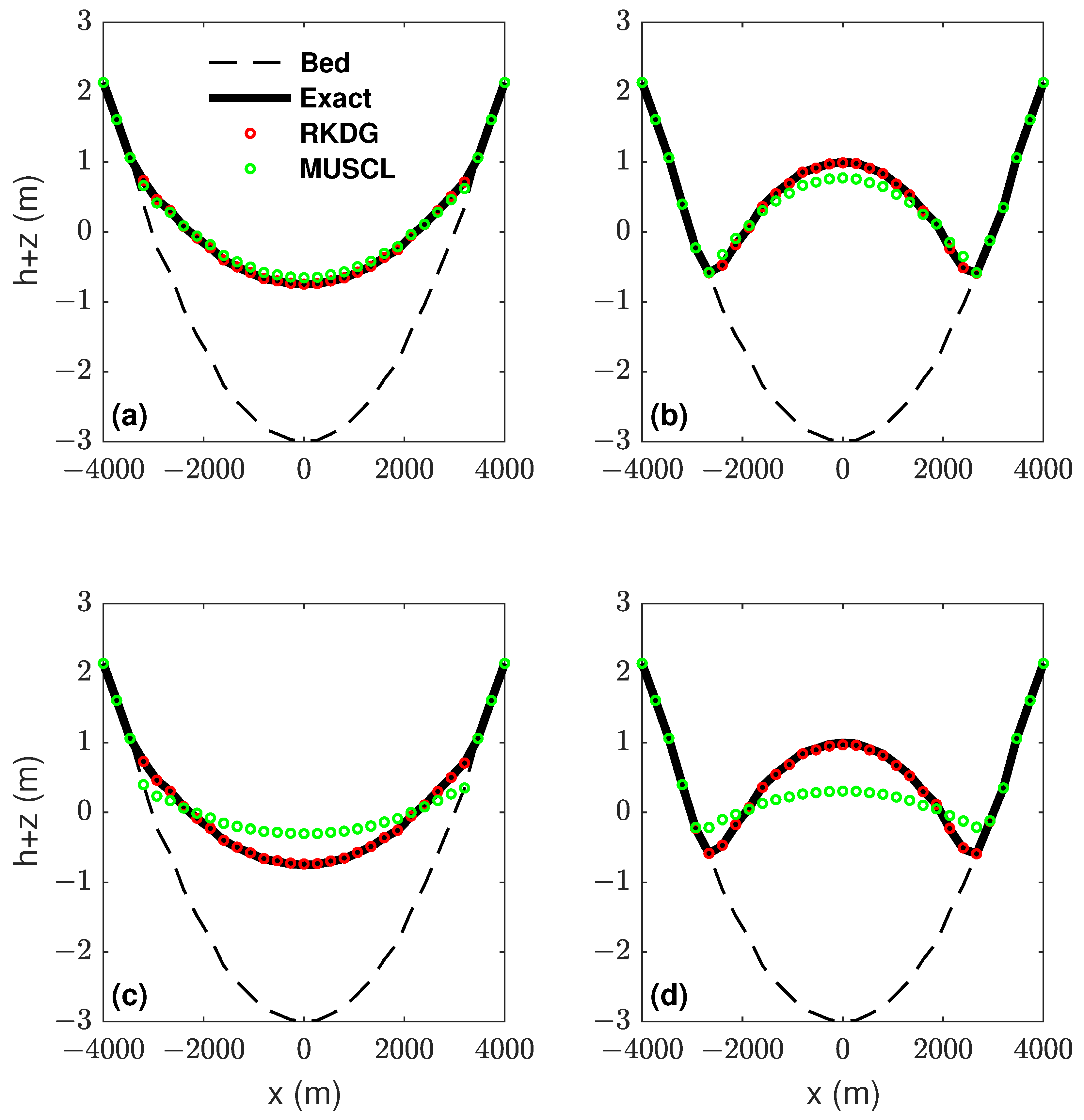
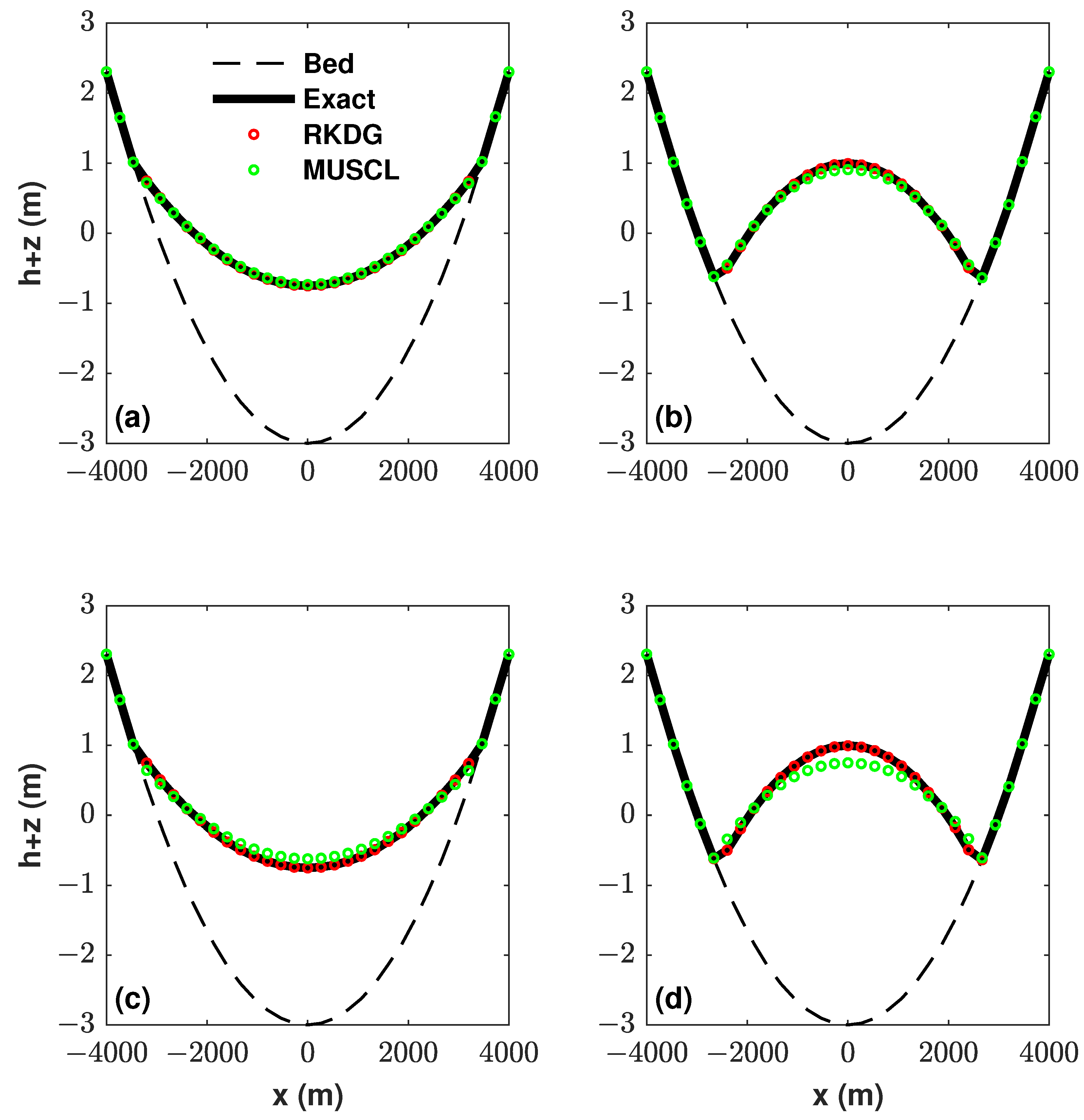
To assess the performance and response of the RKDG and MUSCL models to mesh coarsening, simulations are performed on two meshes made up of 10,048 cells (coarse) and 80,594 cells (fine), respectively, corresponding to a grid resolution of 80 and 30 m. Simulations are carried out for four period cycle $4T$. Figure 2 and Figure 3 display the RKDG and MUSCL water level predictions as well as the analytical solution along the centerline $y=0$. Solutions are presented at four-time intervals, $3T/4$, T, $15T/4$, and $4T$, until four period cycles are accomplished. As Figure 2 and Figure 3 indicate, the mesh coarsening appears to have a significant effect on the accuracy of the MUSCL predictions. On the coarse mesh, the MUSCL scheme gives satisfactory results up to one period cycle (Figure 2a,b). However, for long-duration simulations up to a four period cycle, the MUSCL model lags behind the line of the wetting and drying front during the wetting stage at $15T/4$ (Figure 2a), while it seems to advance too quickly during the drying phase at $4T$ (Figure 2d). In addition, the flow curvature is overestimated at the wetting stages ($3T/4$ and $15T/4$) and underestimated at the dry stages (T and $4T$). Nevertheless, the MUSCL model demonstrates a significantly improved ability to capture the dynamics of the wetting and drying front on the fine mesh (see Figure 3). In contrast, the RKDG scheme delivers accurate predictions of both the moving wet/dry fronts and the flow curvature on both meshes.

For a quantifiable validation, RMSEs for both formulations are calculated after each cycle and listed in

Table 1. Curved flow in a parabolic bowl: RMSE for the water depth at $t=T$ and $t=4T$.

Mesh	MUSCL			RKDG
	Coarse	Fine		Coarse	Fine
$t=T$	7.6 × ${10}^{-2}$	2.1 × ${10}^{-2}$		5.2 × ${10}^{-3}$	7.5 × ${10}^{-4}$
$t=4T$	2.3 × ${10}^{-1}$	7.7 × ${10}^{-2}$		8.1 × ${10}^{-3}$	1.0 × ${10}^{-3}$

. It should be noted that the RKDG model on the coarse mesh outperforms the MUSCL scheme even on the fine mesh. In terms of computational cost, measured runtimes for both solvers are presented in

Table 2. Curved flow in a parabolic bowl: computational time.

	MUSCL	RKDG
Coarse	12.37 s	29.94 s
Fine	157.51 s	366.68 s

. The RKDG method is definitely more computationally demanding than the MUSCL model when applied on the same mesh. The RKDG simulation on the coarse mesh requires around $29.94$ s, while the MUSCL scheme costs $12.37$ s corresponding to a computational time ratio of $2.42$. However, the MUSCL solver takes $157.51$ s to run on the fine mesh, which is approximately about 5 times longer than the RKDG solver on the coarse mesh. In this respect, the RKDG scheme can be considered economically efficient, as it delivers highly accurate results on a coarse mesh, whereas achieving similar accuracy with the MUSCL scheme demands a finer mesh and significantly higher computational costs. Overall, the RKDG solver seems to be a precise and reliable alternative for simulating nonlinear shallow-water flows with wetting and drying on coarse meshes.

4.2. Oblique Hydraulic Jump

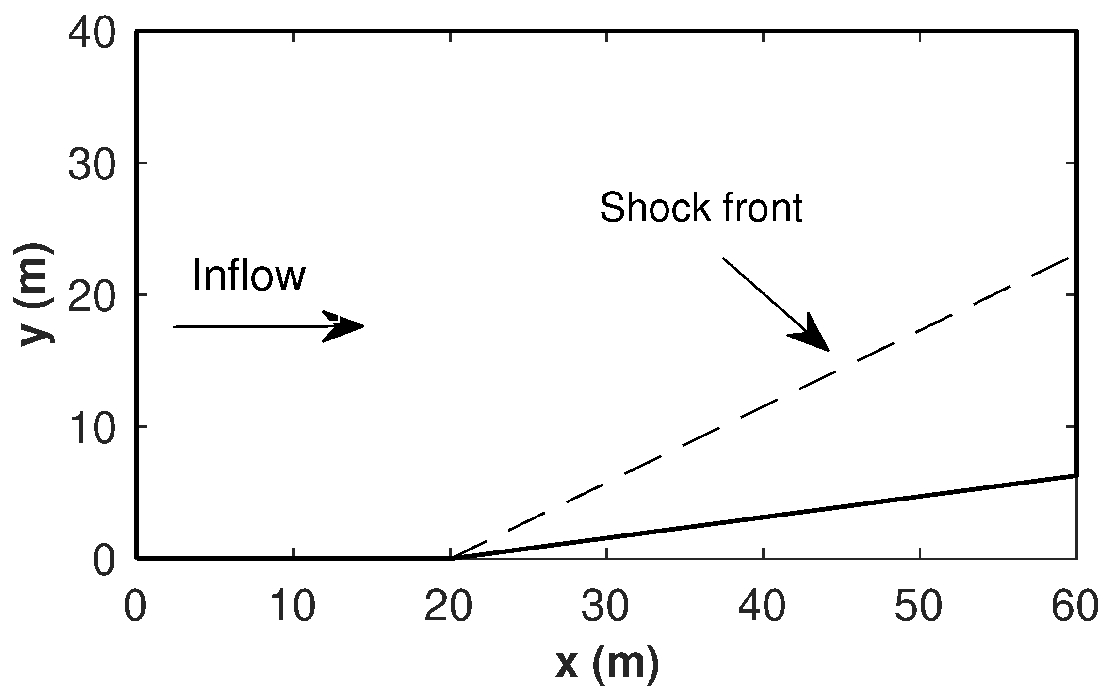
The oblique hydraulic jump is generated by the interaction of a supercritical flow with a converging wall deflected at an angle of 8.95°. This interaction results in the formation of a shock wave at an angle $\beta$. This problem serves as a valuable standard test case to assess the capability of the proposed model to handle high-speed discontinuous flows. The problem domain and a schematic diagram of the induced shock front are illustrated in Figure 4.

The initial and inflow boundary conditions are defined as a flow depth $h_0=1$ m, and velocity components $u_0=8.57$ and $v_0=0$ ${\mathrm{ms}}^{-1}$. A fixed boundary condition is imposed at the upstream boundary, while a free outflow boundary condition is applied at the downstream boundary. A wall boundary condition is enforced along the channel walls. The resulting steady-state flow is expected to remain entirely supercritical, with an oblique hydraulic jump dividing the flow into two regions at an angle of $\beta =30°$ relative to the upstream flow direction. The exact solution downstream of the hydraulic jump is given by a water depth of $1.5$ m and a velocity magnitude of $7.9556$ ${\mathrm{ms}}^{-1}$ [56].

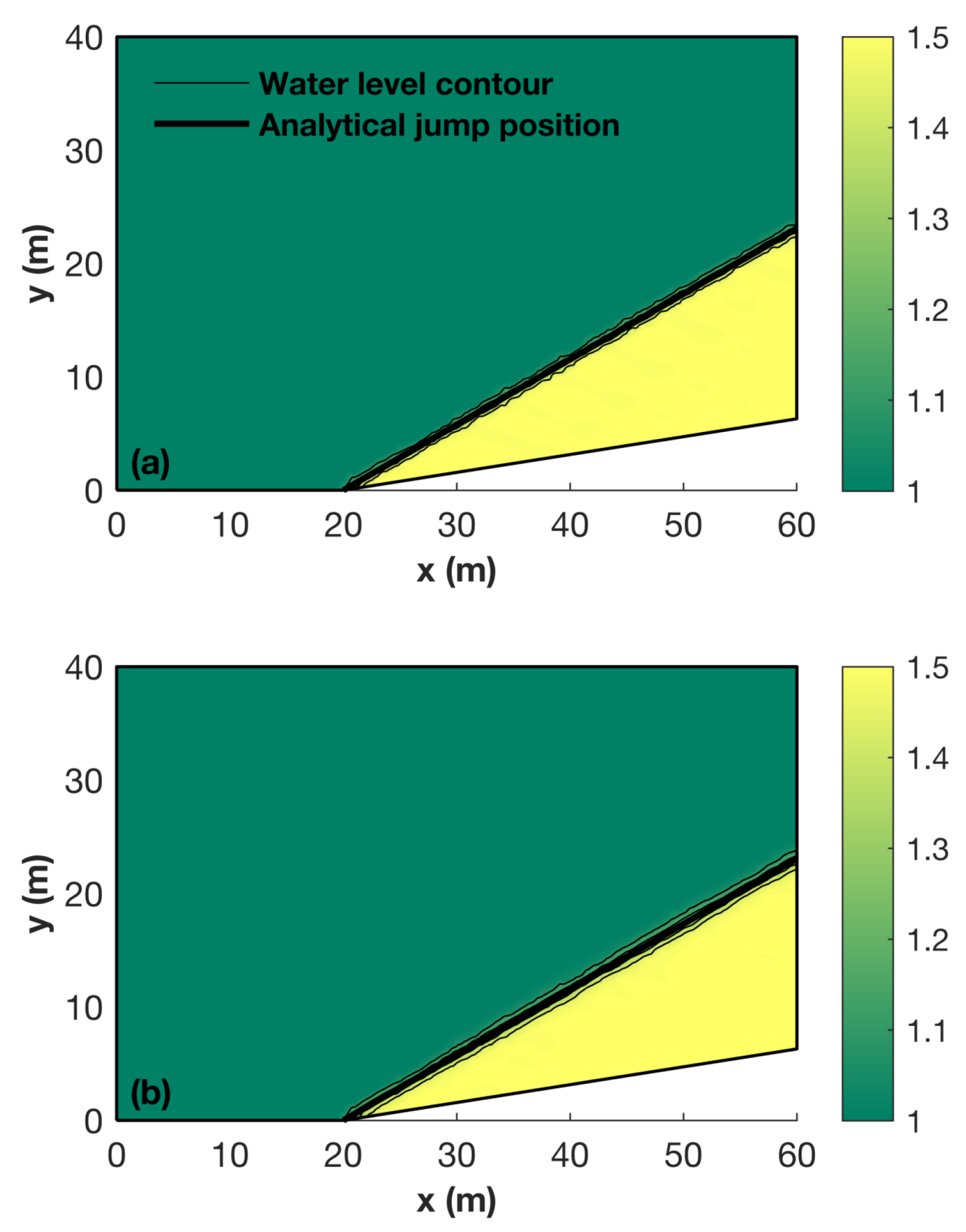
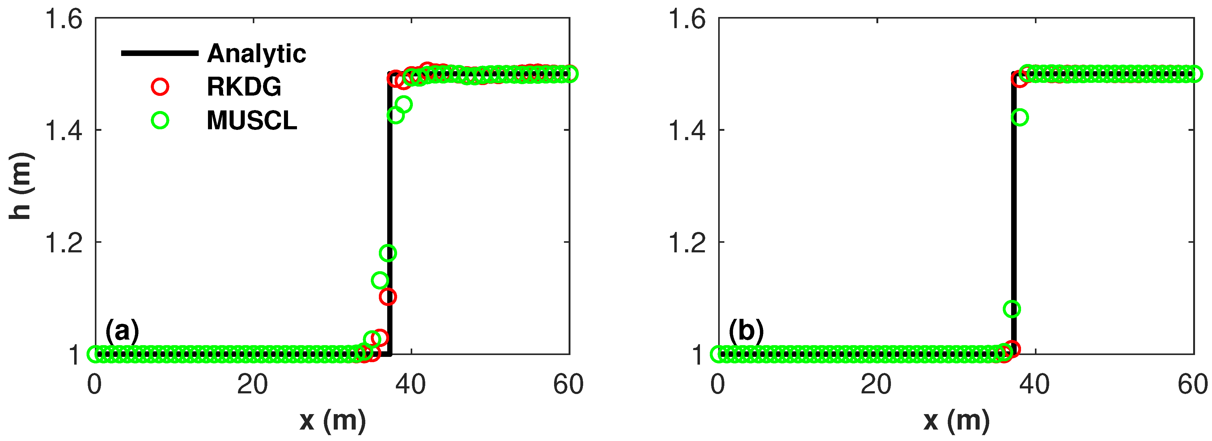
The RKDG and MUSCL models are carried out on two meshes resolution consisting of 10,674 cells (coarse) and 51,821 cells (fine), respectively, corresponding to a grid resolution of $0.5$ and $0.2$ m. Figure 5 illustrates the water depth computed by both schemes on the coarse mesh at $t=30$ s, where the steady-state solutions are attained. The hydraulic jump is well captured by both models and shows good agreement with the analytical position of the jump. However, the RKDG model produces a steeper representation of the jump compared to the MUSCL model. The comparison of the water depth profiles along the horizontal line $y=10$ m is shown in Figure 6. The RKDG scheme demonstrates excellent agreement with the exact solution on both coarse and fine meshes, showcasing its robustness and accuracy. In contrast, the performance of the MUSCL solver is more dependent on the mesh resolution. On the coarse mesh, the MUSCL calculations fail to accurately capture the hydraulic jump and exhibit noticeable oscillations.

For a more detailed analysis,

Table 3. Oblique hydraulic jump: RMSE for the water depth along the line $y=10$ m and CPU time.

Mesh	MUSCL			RKDG
	RMSE	Runtime		RMSE	Runtime
Coarse	3.1 × ${10}^{-2}$	6.78 s		1.5 × ${10}^{-2}$	24.81 s
Fine	1.4 × ${10}^{-2}$	72.25 s		1.6 × ${10}^{-3}$	278.56 s

presents the RMSEs for the RKDG and MUSCL solvers together with the computational runtimes. By analyzing the RMSEs, we can notice that the RKDG scheme on the coarse mesh leads to an error of $0.015$ that is very close to the MUSCL approach on the fine mesh ($0.014$). In terms of computational times, as expected, the RKDG model is substantially slower on the same mesh. On the coarse mesh, the RKDG scheme required approximately $24.81$ s, while the MUSCL scheme completed the computation in just $6.78$ s. However, the MUSCL solver on the fine mesh required a runtime of $72.25$ s, which was about 3 times more than the RKDG solver on the coarse mesh. Despite this, the RKDG model on the coarse mesh remains less costly than the MUSCL scheme on the fine mesh. Overall, the RKDG scheme proves its cost effectiveness by producing accurate simulations on coarse meshes, whereas achieving comparable accuracy with the MUSCL solver necessitates finer meshes and significantly more computational time.

4.3. Toce River Test Case

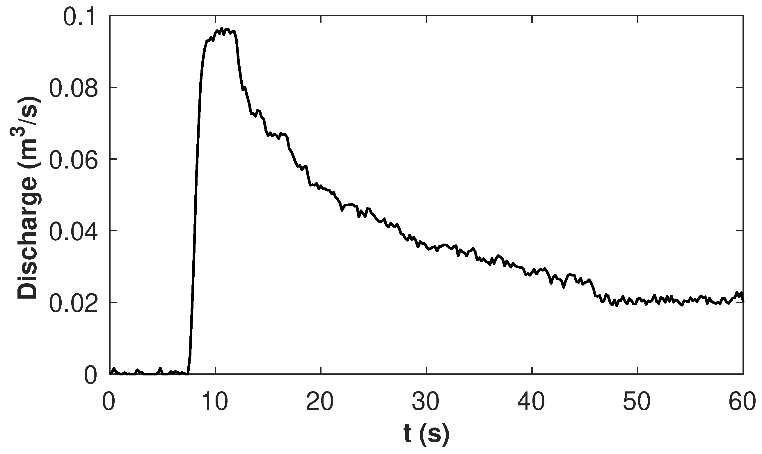
A physical model of the Toce River valley, located in the Northern Alps of Italy, was built to study the propagation of flood waves in urban areas following a dam-break [57]. A 5 km reach of the Toce River valley was scaled down at a ratio of 1:100. The urban area was constructed by placing cubic concrete blocks, each of a length $0.15$ m, representing buildings. These blocks were arranged in two different layouts: aligned and staggered. In this study, the simulation was performed only for the staggered configuration. The time series of water levels were recorded at 10 different gauges in the physical model. The topography of the model as well as the location of experimental gauges are displayed in Figure 7. The domain was initially dry and the flood propagation was controlled by a time-varying discharge released from an upstream reservoir as shown in Figure 8. A free outlet condition was assumed at the downstream boundary and the Manning coefficient was specified as $0.0162$ ${\mathrm{s.m}}^{-1/3}$. Finally, the domain was discretized into 18,400 triangular cells.

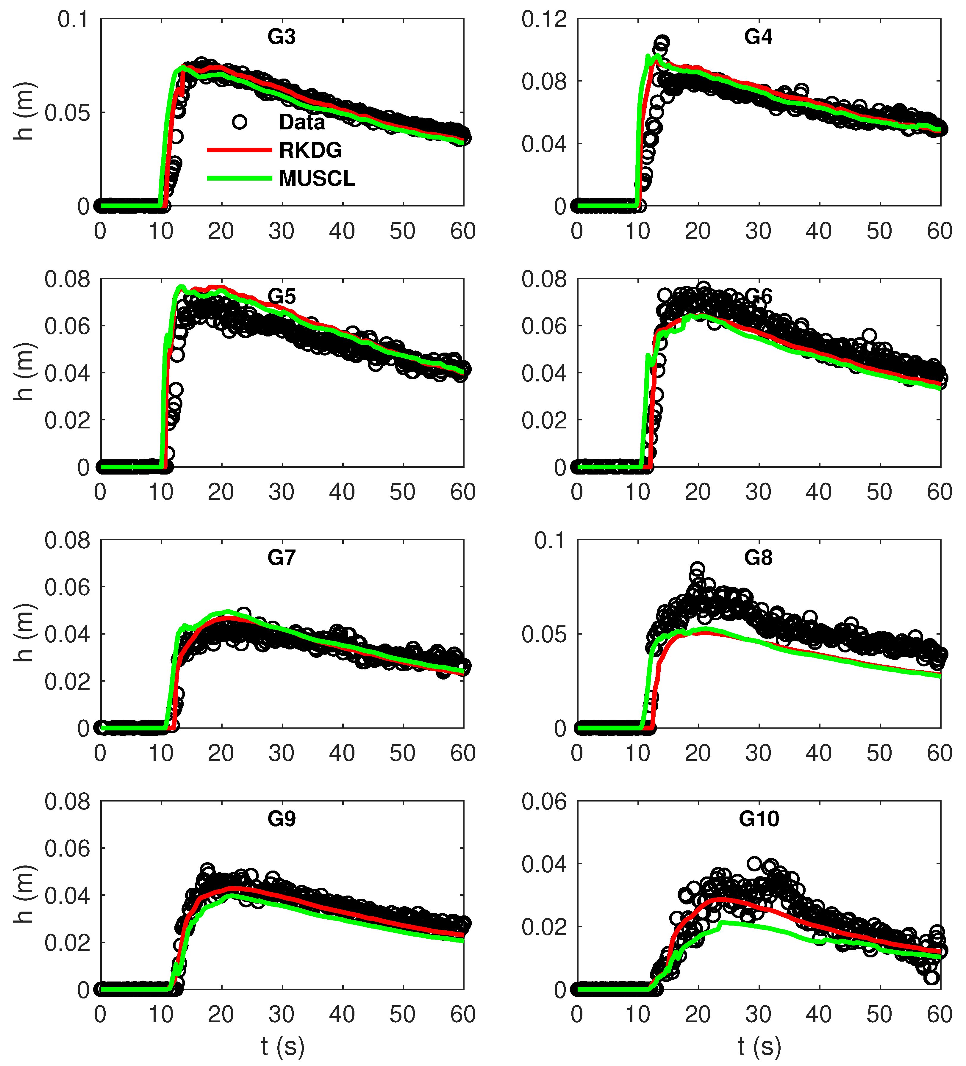
The RKDG and MUSCL models were first run on a coarse mesh formed by 2021 cells. The experimental and predicted time series of water levels at 8 gauges are sketched in Figure 9. The two models show very close predictions and successfully capture the overall trend of the water levels; however, they tend to underestimate the flow depth at G8, likely due to the limitations of the shallow-water equations in representing three-dimensional transient and turbulent flow dynamics. In general, the RKDG model slightly outperforms the MUSCL scheme at most of the gauges. A clear discrepancy appears among the two model predictions at $G10$ located in the exist zone, where the flow is highly variable and changes from subcritical to supercritical in a short distance due to the presence of wake generated by the buildings. The MUSCL scheme clearly underestimates the water level at this gauge, while the RKDG model closely follows the experimental data.

Table 4. Toce River test case: RRMSE (%) for the water depth at the 8 gauges on the coarse mesh.

	G3	G4	G5	G6	G7	G8	G9	G10
RKDG	0.54	1.01	1.07	0.65	0.64	1.54	0.49	1.21
MUSCL	0.98	1.31	1.17	0.99	0.95	1.48	0.97	2.19

summarizes the RRMSE delivered by the two models at the 8 gauges, where lower errors are observed for the RKDG model, especially at $G10$.

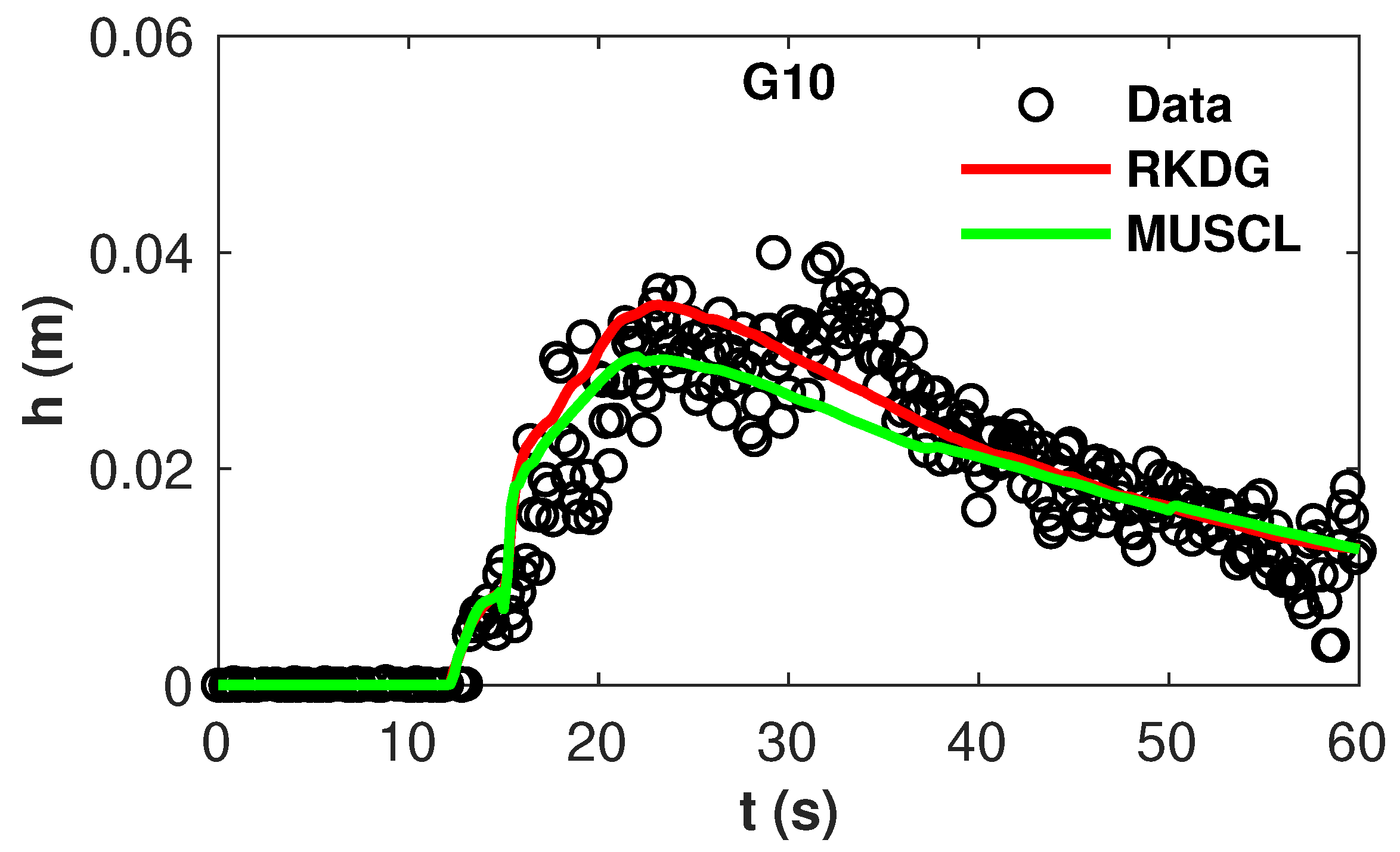
Simulations were undertaken on a fine mesh consisting of 10,653 cells. Figure 10 plots the water level time series computed by the two models at $G10$. The RKDG model is seen to maintain very good agreement compared to the experimental data on both meshes, whereas the performance of the MUSCL scheme appears to be more reliant on the mesh resolution. On the fine mesh, the MUSCL prediction is found to closely match the experimental data and the RKDG profile, and the RRMSEs delivered by the RKDG and MUSCL schemes at $G10$ are $1.18\%$ and $1.21\%$, respectively. It can also be noted that the RKDG model on the coarse mesh provides lower RRMSE at $G10$ than the MUSCL scheme on the fine mesh.

Figure 11 displays the water depth delivered by the RKDG model at $t=20$ s and $t=40$ s. In general, flow features, hydraulic jumps, recirculation, and wake zones are well reproduced by the model. This case study demonstrates that the present model accurately simulates flash flood propagation in urban areas.

4.4. Malpasset Dam-Break

The Malpasset dam was situated on the Reyran River, approximately 12 km upstream of Frejus, a town on the Côte d’Azur, southeastern France. The dam, with a maximum reservoir capacity of $55\times {10}^6$ ${\mathrm{m}}^3$, collapsed in December 1959 following exceptionally heavy rainfall, resulting in the deaths of 421 people and significant damage to downstream areas, including the Esterel freeway. Following the disaster, a police survey was conducted to record maximum water levels across the Reyran River and the arrival times at three electric transformers were also recorded. In addition, a 1:400 scale physical model was constructed to measure flood arrival times and water levels at nine gauges in the floodplain. Due to the complexity of the flow, the Malpasset dam-break problem has been widely studied by many researchers to validate their numerical schemes for modeling flood wave propagation over a complex topography [12,58,59,60,61].

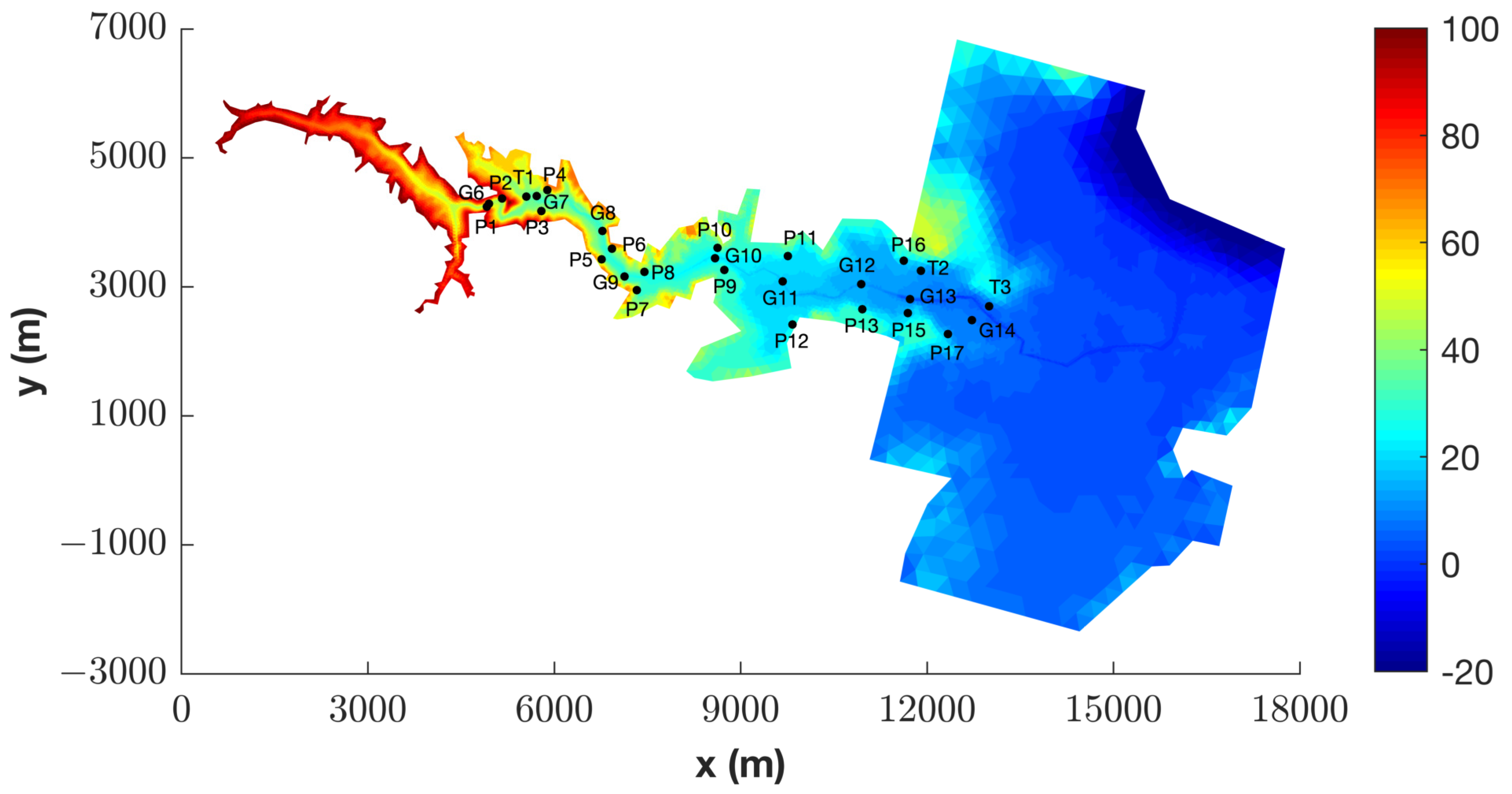
The computational domain was generated in [62] and consists of 26,000 unstructured triangular cells with local refinement near the dam and along the main channel for better accuracy. The mesh resolution ranged from 5 to 50 m. Figure 12 shows the bed topography along with the locations of survey points P and experimental gauges G. The initial water level in the reservoir is set to 100 m, while the rest of the domain is supposed to be dry. A transmissive boundary condition is imposed downstream near the sea and the Manning coefficient is assumed to be $0.033$ ${\mathrm{s.m}}^{-1/3}$ as suggested in [62].

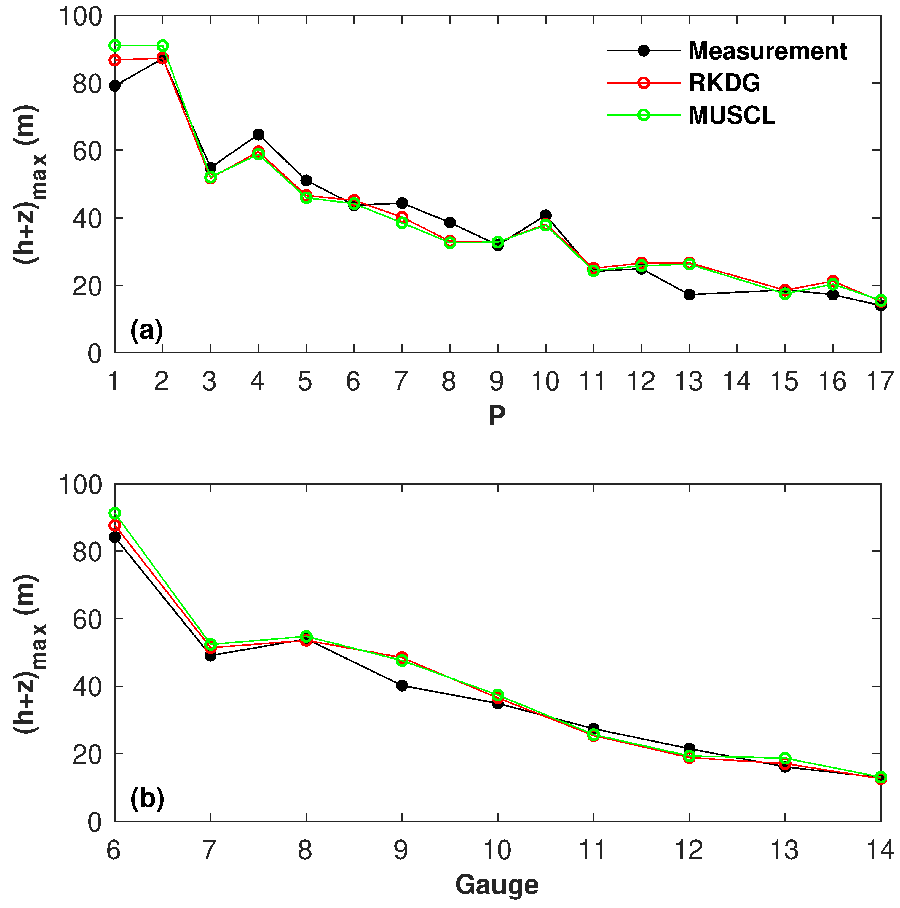
Figure 13 depicts the evolution of the flood wave obtained by the RKDG scheme at $t=1800$ s, when the flood has arrived at the downstream floodplain. The flood path and the reflections and deflections due to irregular bed topography are well reproduced by the model. Maximum water levels observed and computed by the RKDG model at the experimental gauges and survey police points are plotted in Figure 14 and compared to the MUSCL outputs. The results provided by the two models are in good agreement with the survey and data, despite some deviations at $P1$, $P13$, and $G9$, which could be associated with the restrictions of 2D models in modeling 3D flows, modifications in the topography after the event, and uncertainties in the survey and measurements. However, the RKDG model provides slightly better estimation of the water level, notably at $P1$ and $G6$. The RMSEs computed by the RKDG and MUSCL models at $P1$ are $9.60\%$ and $15.12\%$, respectively, while at $G6$, they are $4.16\%$ and $8.43\%$, respectively.

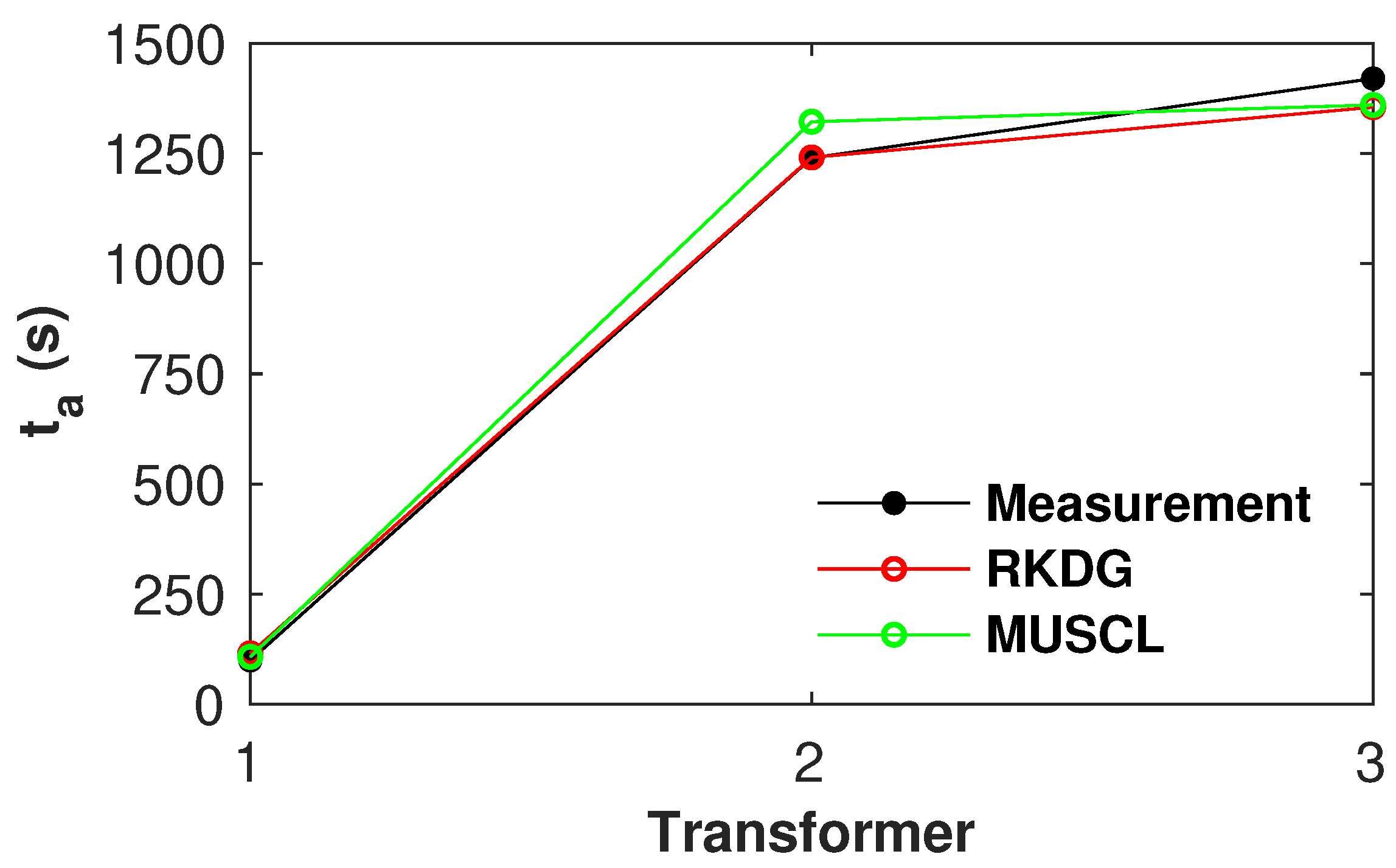
Figure 15 displays the wave arrival times at the three transformers. At $T1$ and $T3$, the arrival times provided by both the RKDG and MUSCL models are very similar, showing a good agreement with the observed values. At $T2$, the RKDG model demonstrates excellent agreement with the measured arrival time, yielding an RRMSE of just $0.08\%$. In contrast, the MUSCL prediction overestimates the measured arrival time, with a corresponding RRMSE $12.74\%$.

Overall, this test problem demonstrates that the proposed model can effectively handle unsteady wet–dry interfaces and complex topography, making it well suited for real-world and large-scale applications.

4.5. Tous Dam-Break

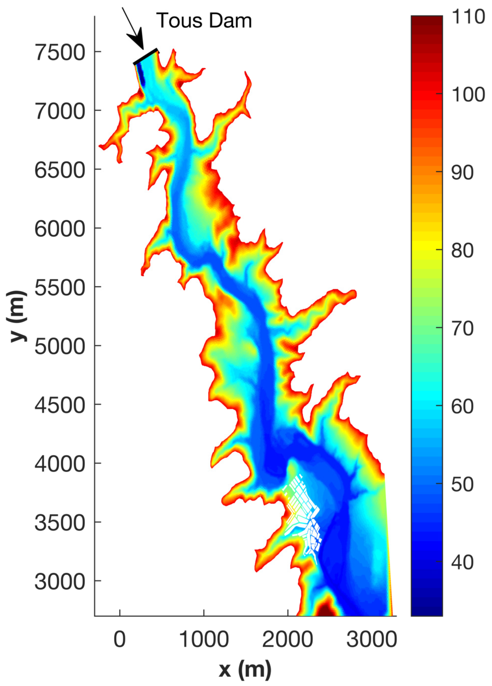
The Tous dam, located on Spain’s Mediterranean coast, is the final flood control structure for the Júcar River basin, which spans approximately 21,600 ${\mathrm{km}}^2$ (Figure 16). On 20–21 October 1982, intense rainfall affected the Tous dam catchment, which covers an area of 17,820 ${\mathrm{km}}^2$), with an average depth of 500 mm. The total rainfall volume in the basin reached nearly 600 million ${\mathrm{m}}^3$, far exceeding the Tous reservoir’s storage capacity of 120 million ${\mathrm{m}}^3$. At 19:00 on 20 October, the Tous dam collapsed, triggering a catastrophic flood wave that inundated many cities situated downstream of the dam. Sumacárcel, a small town located approximately 5 km downstream of the dam, was among the most severely affected areas. The older section of Sumacárcel, located closer to the Júcar river’s right bank, was completely inundated on 20 October 1982. A detailed analysis of the Tous dam failure and the associated dataset is provided in [63].

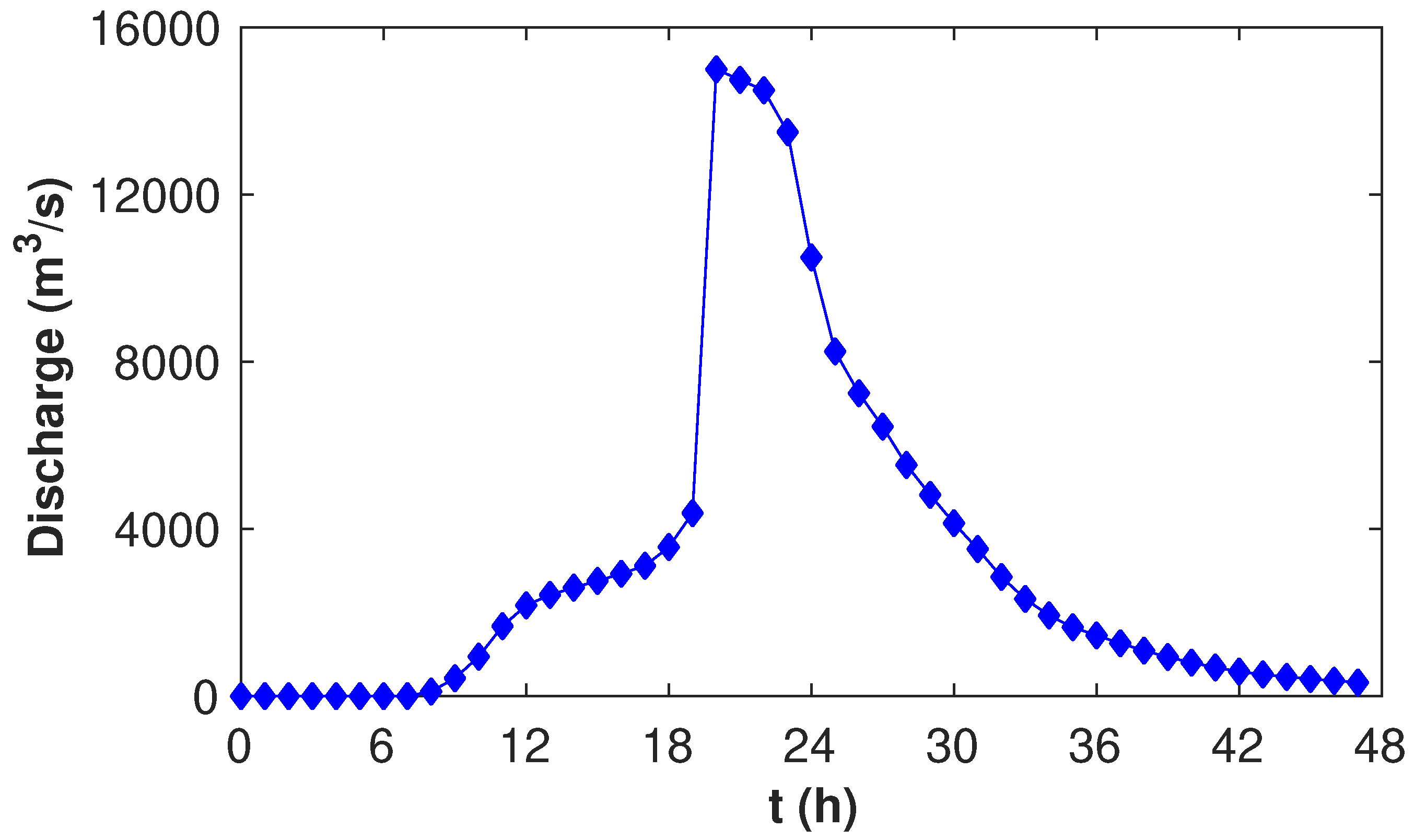
In the numerical simulation, a triangular grid consisting of 25,782 cells is employed, with finer mesh resolution applied to the main river bed and the street of Sumacárcel to enhance accuracy in these critical areas. The mesh resolution varies between $0.5$ m to 50 m. The initial condition assumes a dry bed, while the upstream boundary condition is defined by the flow discharge hydrograph presented in Figure 17. At the downstream boundary, a critical flow condition is imposed. To account for the diversity of soil types, two different values for the Manning roughness coefficient are used: a value of $0.1$ ${\mathrm{s.m}}^{-1/3}$ corresponding to areas with a high friction and $0.03$ ${\mathrm{s.m}}^{-1/3}$ for the remaining parts of the domain, as suggested by [63].

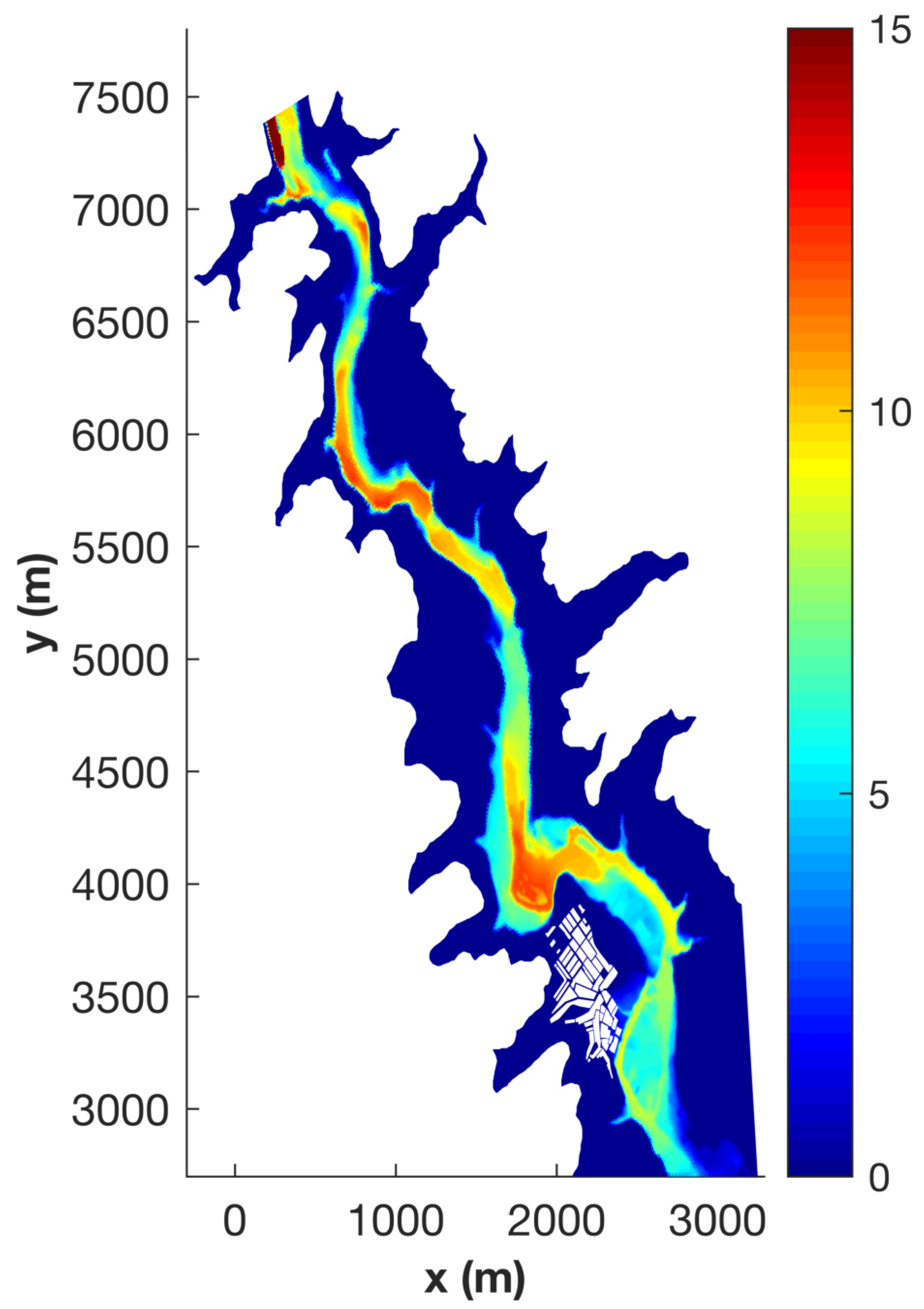
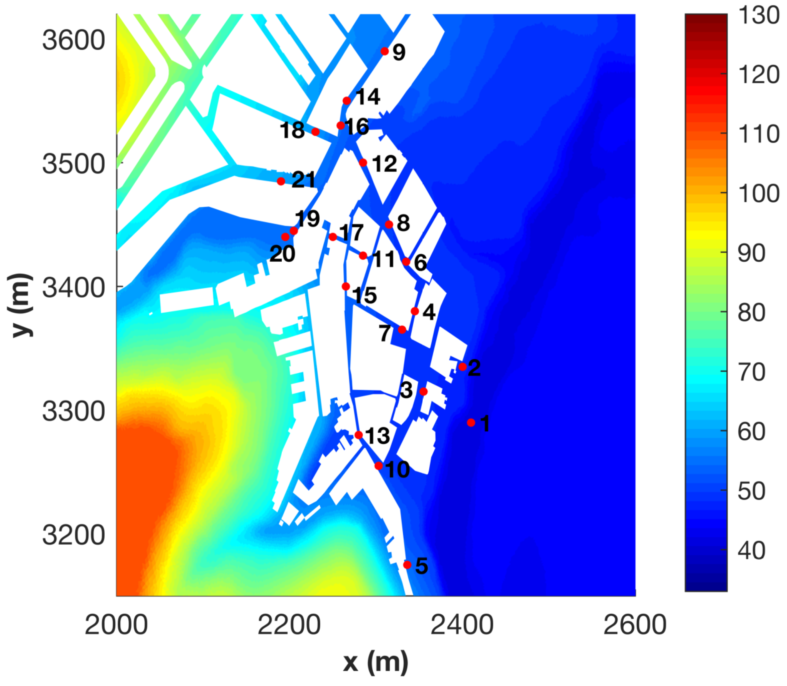
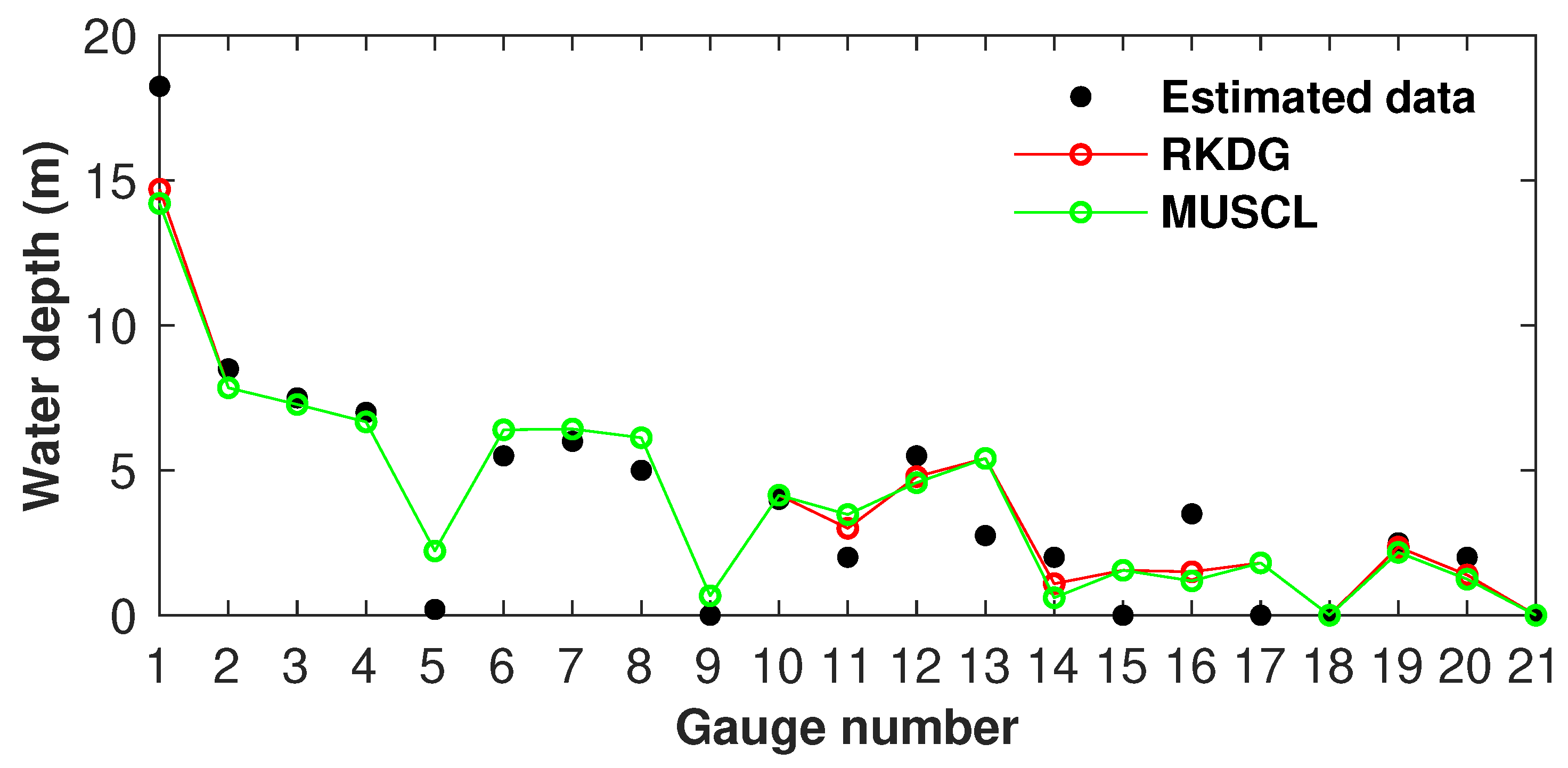
The water depth predicted by the RKDG model after 20 h is illustrated in Figure 18, demonstrating the model’s ability to accurately capture the flow path along the river. Additionally, the models effectively handle reflections and deflections caused by the irregular bed topography. Maximum water level was recorded at 21 locations within or near Sumacárcel (Figure 19). Figure 20 compares the maximum water depth produced by the RKDG model with measurements and survey data, alongside the results obtained from the MUSCL scheme. Both models are found to be very close to each other, and show a good agreement with measurements and police survey despite some discrepancies potentially due to the limitations of 2D models in representing 3D flow dynamics, as well as various sources of uncertainty, including the Manning coefficient, measurement inaccuracies, and changes in the topography after the event.

At gauge 1, the two models underestimate the water level, likely due to its proximity to the upstream boundary, where inflow conditions may carry significant uncertainties [64]. Despite this lower prediction at gauge 1, the RKDG and MUSCL models accurately predict maximum water depths further inside the city at gauges 2, 3, 4, 12, 19, and 20. Similarly, satisfactory predictions are obtained at gauges 5, 6, 7, 8, 9, 10, and 14. Nonetheless, larger discrepancies are observed at gauges 11, 13, 15, 16, and 17. Notably, gauges 18 and 21 recorded no flooding, which aligns with field observations. The RMSEs of the maximum water depth for the RKDG model is $5.23\%$, compared to $5.74\%$ for the MUSCL scheme. The closeness of these results may be attributed to the absence of time series data for water depth and wave arrival times, as maximum water depth alone is not a reliable metric for model comparison. Overall, this test case highlights the potential of the proposed model to accurately simulate long-term urban flash flood evolution over natural terrain.

5. Conclusions

Godunov-type numerical schemes applied to the 2D shallow-water equations on triangular unstructured meshes are particularly useful for modeling flood inundation over complex and irregular domains in real-world applications. This study therefore presents a new nodal RKDG flood model with positivity preservation and wetting and drying on unstructured triangular grids for real-scale flood simulation. The positivity-preserving and wetting and drying approaches proposed by [12] for MUSCL-based models are reviewed and extended to the RKDG solver. First, analytical test problems are used to investigate the performance of the proposed RKDG flood model in contrast with its traditional MUSCL counterpart, focusing particularly on their accuracy, sensitivity to mesh coarsening, and computational cost. Further, the predictive accuracy of the proposed model is explored for three complex and challenging real flood events.

Numerical simulations indicate that the two models generically lead to adequate performance. However, the RKDG scheme shows better accuracy in various benchmark and real-world flood scenarios. The RKDG formulation consistently delivers higher accuracy on coarse meshes, reducing the need for computationally expensive mesh refinement. This advantage is particularly evident in cases involving complex flow features such as moving wet/dry fronts, nonlinear flow curvatures, and hydraulic jumps, where the MUSCL scheme exhibits significant numerical diffusion and mesh-dependence. Nevertheless, the proposed model shows excellent capability in simulating real-world flood events. In general, key flow features, including flood pathways, hydraulic jumps, recirculation zones, and reflections and deflections caused by buildings and irregular topography, are accurately captured by the model. Additionally, the water depths delivered by the model align closely with the experimental data and police survey.

In real-world flood risk management problems, the computational grids are usually dominated by a larger fraction of coarse cells and only a few portions of the grid have refined cells, often limited to urban areas or areas of critical features. In this context, the RKDG model can be favored to maintain the quality of the predictions at large-sized cells, and thereby all over the grid. However, for real-time flood forecasting on grids dominated by small-sized cells, at a resolution less than 15 m, the MUSCL model provides competitive accuracy and is up to 2.5-fold faster for real-world simulations.

References

1. Dottori, F.; Mentaschi, L.; Bianchi, A.; Alfieri, L.; Feyen, L. Cost-effective adaptation strategies to rising river flood risk in Europe. Nat. Clim. Chang. 2023, 13, 196–202. [Google Scholar] [CrossRef]
2. Lhomme, J.; Gutierrez-Andres, J.; Weisgerber, A.; Davison, M.; Mulet-Marti, J.; Cooper, A.; Gouldby, B. Testing a new two-dimensional flood modelling system: Analytical tests and application to a flood event. J. Flood Risk Manag. 2010, 3, 33–51. [Google Scholar] [CrossRef]
3. Neal, J.; Villanueva, I.; Wright, N.; Willis, T.; Fewtrell, T.; Bates, P. How much physical complexity is needed to model flood inundation? Hydrol. Process. 2012, 26, 2264–2282. [Google Scholar] [CrossRef]
4. Mungkasi, S.; Roberts, S. Validation of ANUGA hydraulic model using exact solutions to shallow water wave problems. J. Phys. Conf. Ser. 2013, 423, 012029. [Google Scholar] [CrossRef]
5. BMT-WBM. TUFLOW Classic/HPC User Manual Build 2018-03-AD; WBM Pty Ltd.: Bangalow, NSW, Australia, 2018. [Google Scholar]
6. Wang, Z.J.; Fidkowski, K.; Abgrall, R.; Bassi, F.; Caraeni, D.; Cary, A.; Deconinck, H.; Hartmann, R.; Hillewaert, K.; Huynh, H.T.; et al. High-order CFD methods: Current status and perspective. Int. J. Numer. Methods Fluids 2013, 72, 811–845. [Google Scholar] [CrossRef]
7. Özgen-Xian, I.; Xia, X.; Liang, Q.; Hinkelmann, R.; Liang, D.; Hou, J. Innovations towards the next generation of shallow flow models. Adv. Water Resour. 2021, 149, 103867. [Google Scholar] [CrossRef]
8. Kim, B.; Sanders, B.F.; Schubert, J.E.; Famiglietti, J.S. Mesh type tradeoffs in 2D hydrodynamic modeling of flooding with a Godunov-based flow solver. Adv. Water Resour. 2014, 68, 42–61. [Google Scholar] [CrossRef]
9. Abderrezzak, K.E.K.; Paquier, A.; Mignot, E. Modelling flash flood propagation in urban areas using a two-dimensional numerical model. Nat. Hazards 2009, 50, 433–460. [Google Scholar] [CrossRef]
10. Gallegos, H.A.; Schubert, J.E.; Sanders, B.F. Two-dimensional, high-resolution modeling of urban dam-break flooding: A case study of Baldwin Hills, California. Adv. Water Resour. 2009, 32, 1323–1335. [Google Scholar] [CrossRef]
11. Sanders, B.F.; Schubert, J.E.; Detwiler, R.L. ParBreZo: A parallel, unstructured grid, Godunov-type, shallow-water code for high-resolution flood inundation modeling at the regional scale. Adv. Water Resour. 2010, 33, 1456–1467. [Google Scholar] [CrossRef]
12. Hou, J.; Liang, Q.; Simons, F.; Hinkelmann, R. A 2D well-balanced shallow flow model for unstructured grids with novel slope source term treatment. Adv. Water Resour. 2013, 52, 107–131. [Google Scholar] [CrossRef]
13. Teng, J.; Jakeman, A.J.; Vaze, J.; Croke, B.F.; Dutta, D.; Kim, S. Flood inundation modelling: A review of methods, recent advances and uncertainty analysis. Environ. Model. Softw. 2017, 90, 201–216. [Google Scholar] [CrossRef]
14. Xia, X.; Liang, Q.; Ming, X. A full-scale fluvial flood modelling framework based on a high-performance integrated hydrodynamic modelling system (HiPIMS). Adv. Water Resour. 2019, 132, 103392. [Google Scholar] [CrossRef]
15. Coulibaly, G.; Leye, B.; Tazen, F.; Mounirou, L.A.; Karambiri, H. Urban flood modeling using 2D shallow-water equations in Ouagadougou, Burkina Faso. Water 2020, 12, 2120. [Google Scholar] [CrossRef]
16. Costabile, P.; Costanzo, C.; De Lorenzo, G.; Macchione, F. Is local flood hazard assessment in urban areas significantly influenced by the physical complexity of the hydrodynamic inundation model? J. Hydrol. 2020, 580, 124231. [Google Scholar] [CrossRef]
17. Liu, D.; Tang, J.; Wang, H.; Cao, Y.; Bazai, N.A.; Chen, H.; Liu, D. A new method for wet-dry front treatment in outburst flood simulation. Water 2021, 13, 221. [Google Scholar] [CrossRef]
18. Zhao, J.; Liang, Q. Novel variable reconstruction and friction term discretisation schemes for hydrodynamic modelling of overland flow and surface water flooding. Adv. Water Resour. 2022, 163, 104187. [Google Scholar] [CrossRef]
19. Maranzoni, A.; Tomirotti, M. New formulation of the two-dimensional steep-slope shallow water equations. Part II: Numerical modeling, validation, and application. Adv. Water Resour. 2023, 177, 104403. [Google Scholar] [CrossRef]
20. Peng, F.; Hao, X.; Chai, F. A GPU-Accelerated Two-Dimensional Hydrodynamic Model for Unstructured Grids. Water 2023, 15, 1300. [Google Scholar] [CrossRef]
21. Vallés, P.; Echeverribar, I.; Mairal, J.; Martínez-Aranda, S.; Fernández-Pato, J.; García-Navarro, P. 2D numerical simulation of floods in Ebro river and analysis of boundary conditions to model the Mequinenza reservoir dam. GeoHazards 2023, 4, 136–156. [Google Scholar] [CrossRef]
22. Ferrari, A. A parallel porosity model for large-scale modelling of river floods in urban areas. J. Hydrol. 2024, 635, 131232. [Google Scholar] [CrossRef]
23. Wang, J.; Hou, J.; Li, S.; Sun, J.; Jing, J.; Wang, J. Advancements in enhancing flood evolution and urban inundation predictions: A study of local time stepping algorithm and GPU-accelerated hydrodynamic model. J. Hydrol. 2024, 641, 131744. [Google Scholar] [CrossRef]
24. Van Leer, B. Towards the ultimate conservative difference scheme. V. A second-order sequel to Godunov’s method. J. Comput. Phys. 1979, 32, 101–136. [Google Scholar] [CrossRef]
25. Ayog, J.L.; Kesserwani, G.; Shaw, J.; Sharifian, M.K.; Bau, D. Second-order discontinuous Galerkin flood model: Comparison with industry-standard finite volume models. J. Hydrol. 2021, 594, 125924. [Google Scholar] [CrossRef]
26. Ghostine, R.; Kesserwani, G.; Vazquez, J.; Rivière, N.; Ghenaim, A.; Mose, R. Simulation of supercritical flow in crossroads: Confrontation of a 2D and 3D numerical approaches to experimental results. Comput. Fluids 2009, 38, 425–432. [Google Scholar] [CrossRef]
27. Xing, Y.; Zhang, X.; Shu, C.W. Positivity-preserving high order well-balanced discontinuous Galerkin methods for the shallow water equations. Adv. Water Res. 2010, 33, 1476–1493. [Google Scholar] [CrossRef]
28. Duran, A.; Marche, F. Recent advances on the discontinuous Galerkin method for shallow water equations with topography source terms. Comput. Fluids 2014, 101, 88–104. [Google Scholar] [CrossRef]
29. Wirasaet, D.; Kubatko, E.; Michoski, C.; Tanaka, S.; Westerink, J.; Dawson, C. Discontinuous Galerkin methods with nodal and hybrid modal/nodal triangular, quadrilateral, and polygonal elements for nonlinear shallow water flow. Comput. Methods Appl. Mech. Eng. 2014, 270, 113–149. [Google Scholar] [CrossRef]
30. Caviedes-Voullième, D.; Kesserwani, G. Benchmarking a multiresolution discontinuous Galerkin shallow water model: Implications for computational hydraulics. Adv. Water Resour. 2015, 86, 14–31. [Google Scholar] [CrossRef]
31. Kesserwani, G.; Ayog, J.L.; Bau, D. Discontinuous Galerkin formulation for 2D hydrodynamic modelling: Trade-offs between theoretical complexity and practical convenience. Comput. Methods Appl. Mech. Eng. 2018, 342, 710–741. [Google Scholar] [CrossRef]
32. Faghih-Naini, S.; Kuckuk, S.; Zint, D.; Kemmler, S.; Köstler, H.; Aizinger, V. Discontinuous Galerkin method for the shallow water equations on complex domains using masked block-structured grids. Adv. Water Resour. 2023, 182, 104584. [Google Scholar] [CrossRef]
33. Kesserwani, G.; Wang, Y. Discontinuous Galerkin flood model formulation: Luxury or necessity? Water Resour. Res. 2014, 50, 6522–6541. [Google Scholar] [CrossRef]
34. Samii, A.; Michoski, C.; Dawson, C. A parallel and adaptive hybridized discontinuous Galerkin method for anisotropic nonhomogeneous diffusion. Comput. Methods Appl. Mech. Eng. 2016, 304, 118–139. [Google Scholar] [CrossRef]
35. Fuhry, M.; Giuliani, A.; Krivodonova, L. Discontinuous Galerkin methods on graphics processing units for nonlinear hyperbolic conservation laws. Int. J. Numer. Methods Fluids 2014, 76, 982–1003. [Google Scholar] [CrossRef]
36. Brus, S.; Wirasaet, D.; Westerink, J.J.; Dawson, C. Performance and scalability improvements for discontinuous Galerkin solutions to conservation laws on unstructured grids. J. Sci. Comput. 2017, 70, 210–242. [Google Scholar] [CrossRef]
37. Ern, A.; Piperno, S.; Djadel, K. A well-balanced Runge–Kutta discontinuous Galerkin method for the shallow-water equations with flooding and drying. Int. J. Numer. Methods Fluids 2008, 58, 1–25. [Google Scholar] [CrossRef]
38. Xing, Y.; Zhang, X. Positivity-preserving well-balanced discontinuous Galerkin methods for the shallow water equations on unstructured triangular meshes. J. Sci. Comput. 2013, 57, 19–41. [Google Scholar] [CrossRef]
39. Zhang, X.; Xia, Y.; Shu, C.W. Maximum-principle-satisfying and positivity-preserving high order discontinuous Galerkin schemes for conservation laws on triangular meshes. J. Sci. Comput. 2012, 50, 29–62. [Google Scholar] [CrossRef]
40. Li, L.; Zhang, Q. A new vertex-based limiting approach for nodal discontinuous Galerkin methods on arbitrary unstructured meshes. Comput. Fluids 2017, 159, 316–326. [Google Scholar] [CrossRef]
41. Vater, S.; Beisiegel, N.; Behrens, J. A limiter-based well-balanced discontinuous Galerkin method for shallow-water flows with wetting and drying: Triangular grids. Int. J. Numer. Methods Fluids 2019, 91, 395–418. [Google Scholar] [CrossRef]
42. Dutt, K.; Krivodonova, L. A high-order moment limiter for the discontinuous Galerkin method on triangular meshes. J. Comput. Phys. 2021, 433, 110188. [Google Scholar] [CrossRef]
43. Bunya, S.; Kubatko, E.J.; Westerink, J.J.; Dawson, C. A wetting and drying treatment for the Runge–Kutta discontinuous Galerkin solution to the shallow water equations. Comput. Methods Appl. Mech. Eng. 2009, 198, 1548–1562. [Google Scholar] [CrossRef]
44. Brufau, P.; García-Navarro, P.; Vázquez-Cendón, M. Zero mass error using unsteady wetting–drying conditions in shallow flows over dry irregular topography. Int. J. Numer. Methods Fluids 2004, 45, 1047–1082. [Google Scholar] [CrossRef]
45. Kärnä, T.; De Brye, B.; Gourgue, O.; Lambrechts, J.; Comblen, R.; Legat, V.; Deleersnijder, E. A fully implicit wetting–drying method for DG-FEM shallow water models, with an application to the Scheldt Estuary. Comput. Methods Appl. Mech. Eng. 2011, 200, 509–524. [Google Scholar] [CrossRef]
46. Audusse, E.; Bouchut, F.; Bristeau, M.O.; Klein, R.; Perthame, B. A fast and stable well-balanced scheme with hydrostatic reconstruction for shallow water flows. J. Sci. Comput. 2004, 25, 2050–2065. [Google Scholar] [CrossRef]
47. Kesserwani, G.; Sharifian, M.K. (Multi) wavelets increase both accuracy and efficiency of standard Godunov-type hydrodynamic models: Robust 2D approaches. Adv. Water Resour. 2020, 144, 103693. [Google Scholar] [CrossRef]
48. Shaw, J.; Kesserwani, G.; Neal, J.; Bates, P.; Sharifian, M.K. LISFLOOD-FP 8.0: The new discontinuous Galerkin shallow water solver for multi-core CPUs and GPUs. Geosci. Model Dev. 2020, 14, 3577–3602. [Google Scholar] [CrossRef]
49. Lai, W.; Khan, A.A. Modeling dam-break flood over natural rivers using discontinuous Galerkin method. J. Hydrodyn. 2012, 24, 467–478. [Google Scholar] [CrossRef]
50. Filippini, A.G.; Arpaia, L.; Perrier, V.; Pedreros, R.; Bonneton, P.; Lannes, D.; Marche, F.; De Brye, S.; Delmas, S.; Lecacheux, S.; et al. An operational discontinuous Galerkin shallow water model for coastal flood assessment. Ocean Model. 2024, 192, 102447. [Google Scholar] [CrossRef]
51. Wichitrnithed, C.; Valseth, E.; Kubatko, E.J.; Kang, Y.; Hudson, M.; Dawson, C. A discontinuous Galerkin finite element model for compound flood simulations. Comput. Methods Appl. Mech. Eng. 2024, 420, 116707. [Google Scholar] [CrossRef]
52. Toro, E.F. Riemann Solvers and Numerical Methods for Fluid Dynamics: A Practical Introduction, 3rd ed.; Springer: Berlin/Heidelberg, Germany, 2009. [Google Scholar]
53. Cockburn, B.; Shu, C.W. The Runge–Kutta discontinuous Galerkin method for conservation laws V: Multidimensional systems. J. Comput. Phys. 1998, 141, 199–224. [Google Scholar] [CrossRef]
54. Xing, Y.; Shu, C.W. A new approach of high order well-balanced finite volume WENO schemes and discontinuous Galerkin methods for a class of hyperbolic systems with source terms. Commun. Comput. Phys. 2006, 1, 100–134. [Google Scholar]
55. Begnudelli, L.; Sanders, B.F. Unstructured grid finite-volume algorithm for shallow-water flow and scalar transport with wetting and drying. J. Hydraul. Eng. 2006, 132, 371–384. [Google Scholar] [CrossRef]
56. Alcrudo, F.; Garcia-Navarro, P. A high-resolution Godunov-type scheme in finite volumes for the 2D shallow-water equations. Int. J. Numer. Methods Fluids 1993, 16, 489–505. [Google Scholar] [CrossRef]
57. Testa, G.; Zuccala, D.; Alcrudo, F.; Mulet, J.; Soares-Frazão, S. Flash flood flow experiment in a simplified urban district. J. Hydraul. Res. 2007, 45, 37–44. [Google Scholar] [CrossRef]
58. Valiani, A.; Caleffi, V.; Zanni, A. Case study: Malpasset dam-break simulation using a two-dimensional finite volume method. J. Hydraul. Eng. 2002, 128, 460–472. [Google Scholar] [CrossRef]
59. Huang, Y.; Zhang, N.; Pei, Y. Well-balanced finite volume scheme for shallow water flooding and drying over arbitrary topography. Eng. Appl. Comput. Fluid Mech. 2013, 7, 40–54. [Google Scholar] [CrossRef]
60. Biscarini, C.; Di Francesco, S.; Ridolfi, E.; Manciola, P. On the simulation of floods in a narrow bending valley: The malpasset dam break case study. Water 2016, 8, 545. [Google Scholar] [CrossRef]
61. Wu, G.f.; He, Z.g.; Zhao, L.; Liu, G.h. A well-balanced positivity preserving two-dimensional shallow flow model with wetting and drying fronts over irregular topography. J. Hydrodyn. 2018, 30, 618–631. [Google Scholar] [CrossRef]
62. Goutal, N. The Malpasset dam failure. An overview and test case definition. In Proceedings of the 4th CADAM Meeting, Zaragoza, Spain, 18–19 November 1999. [Google Scholar]
63. Alcrudo, F.; Mulet, J. Description of the Tous Dam break case study (Spain). J. Hydraul. Res. 2007, 45, 45–57. [Google Scholar] [CrossRef]
64. Mulet, J.; Alcrudo, F. Uncertainty analysis of Tous flood propagation case study. In Proceedings of the 4rd IMPACT Project Workshop, Málaga, Spain, 10–12 November 2004. [Google Scholar]
Figure 1. The quadrature points within a triangular element. G i ( i = 1 , 2 , and 3) represent the local Gauss quadrature points used to approximate the volume integral terms in Equation (6). G f j ( f = 1 , 2 , and 3; j = 1 and 2) are Gaussian points for aggregating the normal Riemann fluxes in Equation (6).
Water 17 01141 g001
Figure 2. Curved flow in a parabolic bowl: water level computed by the RKDG and MUSCL schemes on the coarse mesh: (a) t = 3 T / 4 ; (b) t = T ; (c) t = 15 T / 4 ; (d) t = 4 T .
Water 17 01141 g002
Figure 3. Curved flow in a parabolic bowl: water level computed by the RKDG and MUSCL schemes on the fine mesh: (a) t = 3 T / 4 ; (b) t = T ; (c) t = 15 T / 4 ; (d) t = 4 T .
Water 17 01141 g003
Figure 4. Oblique hydraulic jump: computational domain.
Water 17 01141 g004
Figure 5. Oblique hydraulic jump: computed water depth contour on coarse mesh at t = 30 s: (a) RKDG; (b) MUSCL.
Water 17 01141 g005
Figure 6. Oblique hydraulic jump: comparison between analytical and numerical water depth profiles delivered by RKDG and MUSCL schemes along horizontal line y = 10 m: (a) coarse mesh; (b) fine mesh.
Water 17 01141 g006
Figure 7. Toce River test case: physical domain showing the topography and the location of buildings (white squares) and 8 gauging points.
Water 17 01141 g007
Figure 8. Toce River test case: inflow hydrograph applied as upstream boundary condition.
Water 17 01141 g008
Figure 9. Toce River test case: experimental and numerical water level profiles on the coarse mesh at different gauges.
Water 17 01141 g009
Figure 10. Toce River test case: experimental and numerical water level profiles on the fine mesh at gauge G 10 .
Water 17 01141 g010
Figure 11. Toce River test case: water depth maps predicted by the RKDG solver at (a) t = 20 s and (b) t = 40 s.
Water 17 01141 g011
Figure 12. Malpasset dam-break: topography and locations of the experimental gauges and survey points.
Water 17 01141 g012
Figure 13. Malpasset dam-break: computed water depth by the RKDG scheme at t = 1800 s.
Water 17 01141 g013
Figure 14. Malpasset dam-break: maximum water level observed and computed by the RKDG model at (a) experimental gauges and (b) police survey points.
Water 17 01141 g014
Figure 15. Malpasset dam-break: arrival times ( t a ) at the three electric transformers.
Water 17 01141 g015
Figure 16. Topography of the Tous dam problem showing the location of the dam, Júcar River, and the town of Sumacárcel.
Water 17 01141 g016
Figure 17. Tous dam-break: inflow hydrograph imposed as upstream boundary condition.
Water 17 01141 g017
Figure 18. Tous dam-break: water depth predicted by the RKDG model after 20 h.
Water 17 01141 g018
Figure 19. Tous dam-break: gauge locations in the streets of Sumacárcel.
Water 17 01141 g019
Figure 20. Tous dam-break: maximum water depth measured and computed by the RKDG and MUSCL solvers at different gauges in the town of Sumacárcel.
Water 17 01141 g020