Abstract
Stokes drift refers to the net horizontal displacement of water particles under the influence of wave action, playing a crucial role in the transport of heat, salt, nutrients, and pollutants in the ocean. Accurate estimation of Stokes drift is essential for understanding ocean dynamics and material transport. This study utilizes two deep learning models (Earthformer and ConvLSTM) to predict surface Stokes drift, using wind and water depth as input variables. We designed three control experiments to evaluate the impact of different training objectives on the experimental results. In Exp. 1, the model used the two Stokes drift components (us, vs) as the training objectives. In Exp. 2, the objectives were the two components (us, vs) plus the direction θ. In Exp. 3, the model employed the magnitude and the direction of the Stokes drift as the training objectives. The results indicate that using the magnitude and direction (Exp. 3) significantly reduces the RMSE for magnitude, direction, and each component (us, vs) by up to 33.3%, compared to the other two strategies. Moreover, the approach of choosing magnitude and direction as the training objectives can also be applied to the prediction of other vector variables, such as ocean currents and winds.
1. Introduction
A particle floating on the free surface of a water wave experiences a net drift velocity in the direction of wave propagation, known as the Stokes drift [1]. This phenomenon was first discovered by George Stokes in 1847, primarily caused by the asymmetry of wave shapes. More generally, the Stokes drift velocity is the difference between the Lagrangian velocity and the Eulerian velocity [2].
Stokes drift is one of the most important mechanisms for material transport in the ocean. It facilitates the horizontal transport of nutrients, oxygen, plankton, heat, and other suspended particles. Within coral reef hydrodynamics, Stokes drift promotes the delivery of nutrients and oxygen into reef ecosystems [3]. It drives the onshore transport of planktonic larvae and other organisms near the ocean surface, as well as offshore transport at intermediate depths [4,5]. Additionally, Stokes drift significantly influences mixed-layer temperature variability by providing an advective heat transport component. Particularly at mid-to-high latitudes, its contribution to heat fluxes can be comparable to that of mean ocean currents [6,7].
Besides promoting the circulation and horizontal transport of materials, Stokes drift also plays a crucial role in the dispersion and migration pathways of oil spills, suspended particles, and other pollutants. Its magnitude can be of the same order as Eulerian currents, meaning that, when incorporated into adjacency matrix-based long-term predictions, particle concentrations in subtropical ocean garbage patches can decrease by a full order of magnitude within a century [8]. Given its similarity in magnitude and directional characteristics to wind-driven drift [9], studies have shown that incorporating Stokes drift into oil spill models significantly improves prediction accuracy for medium- to long-term (beyond two days) spill scenarios [10]. Stokes drift is also a critical factor in predicting drifting trajectories [11].
As a core component of wave momentum balance, Stokes drift similarly plays a crucial role in the coastal and mixed-layer dynamical processes [12,13,14,15,16]. Through interaction with the Coriolis force, it introduces a lateral (rotational) velocity component that is in phase with vertical velocity. Variations in Stokes drift, associated with wave growth or decay, trigger momentum exchanges between the wave field and mean flows [17]. It has been demonstrated that, by modifying the surface-layer stability parameter, Stokes drift is more effective in reducing vertical shear than stratification alone [18,19]. Tamura et al. showed that the vertical surface velocities induced by the divergence in Stokes drift can be comparable to Ekman velocities and may even alter mesoscale frontal dynamics [20]. Furthermore, Stokes drift is indispensable in the turbulence generation mechanism associated with Langmuir circulation [21]. It contributes to the formation of Langmuir turbulence, thereby enhancing vertical mixing and deepening the mixed layer [22,23,24].
Given the critical role of Stokes drift in ocean dynamics, accurately estimating it has become an important research topic. Historically, estimates of Stokes drift have been achieved through empirical formulas [25,26]. One common approach involves calculating Stokes drift velocity based on directional wave energy spectra, which can be obtained from wave buoys and wave models [27]. However, estimating Stokes drift and its profile from wave buoys is challenging, mainly due to the uncertainty of handling the effects of directional spreading [28]. Additionally, the estimation of Stokes drift using wave models is often limited by unresolved physical aspects, such as nonlinear wave interactions and wave dissipation [2].
With the rapid growth of ocean big data and the continuous maturation of artificial intelligence methods, AI technology has been widely applied in the field of ocean science due to its outstanding ability to simulate nonlinear behavior in complex physical systems. Cutting-edge techniques, such as data-driven deep learning approaches, have demonstrated unique and significant advantages in predicting ocean phenomena such as surface waves [29,30,31,32,33,34,35]. As mentioned above, Stokes drift plays a crucial role in ocean dynamics. However, traditional numerical wave models are computationally expensive, particularly at high resolutions, and prone to cumulative errors due to incomplete descriptions of physical processes. Given these limitations, machine learning techniques have been applied to predict surface Stokes drift and have proven that these models can more accurately capture the complex relationships among multiple input variables [36]. Nevertheless, to date, research explicitly utilizing deep learning models to predict Stokes drift remains relatively unexplored. In regional prediction tasks, which involve multidimensional spatiotemporal data such as latitude, longitude, time, and oceanic parameters, traditional machine learning often relies on feature engineering to reduce high-dimensional data to a two-dimensional matrix. This process inevitably leads to the loss of some spatial correlations (e.g., local dynamic coupling effects), thereby limiting the model’s ability to capture complex interactions within a region. In contrast, deep learning models can automatically extract hierarchical and complex features, effectively capturing the inherent nonlinearities and spatiotemporal variability of ocean processes, which gives them a significant advantage in handling regional prediction tasks. This capability is particularly valuable for predicting Stokes drift, given its highly nonlinear and spatiotemporally complex characteristics. Although advanced deep learning models, such as ConvLSTM (Convolutional Neural Network) and Earthformer (Earth System Forecasting Transformer), have recently been developed, they have not yet been applied to Stokes drift prediction, to the best of our knowledge.
The temporal prediction model, ConvLSTM, integrates CNN (Convolutional Neural Network) and LSTM (Long Short-Term Memory), thereby overcoming the respective limitations of traditional CNNs and RNNs (Recurrent Neural Network) [37]. The ConvLSTM model structure is mainly divided into two parts: it follows the typical RNN architecture for temporal structures and adopts the CNN feature extraction approach for spatial structures. The Earthformer model is based on the Transformer architecture, specifically designed for data prediction and analysis in the field of Earth sciences [38]. Earthformer leverages self-attention mechanisms to capture and process complex dependencies within spatiotemporal data more effectively. This makes it particularly advantageous for handling multivariate time series data in ocean dynamics and weather prediction. The advancement of transformer models has significantly enhanced predictive capabilities in oceanic and atmospheric sciences. Given the rapid development and widespread application of deep learning in oceanography, as well as the critical importance of accurately predicting Stokes drift, in this study, we applied Earthformer and ConvLSTM models to predict surface Stokes drift.
The structure of this paper is as follows: The experimental configurations are described in Section 2. The Stokes drift predictions from the deep learning model are presented in Section 3. Section 4 provides a detailed discussion, and finally, Section 5 summarizes the conclusions and broader implications.
2. Experimental Configurations
2.1. Data
This study focused on the northern part of the South China Sea, specifically between 14° N and 23° N and between 106° E and 126° E. The data used in this study covered a period of ten years, from January 2013 to December 2022, including the wind velocity and surface Stokes drift velocity from the Copernicus Marine Environment Monitoring Service (CMEMS), as well as depth data provided by ETOPO (ETOPO Global Relief Model). To ensure consistency, all data were uniformly interpolated onto the Stokes drift grid (0.2° × 0.2° spatial resolution and 3 h temporal resolution) before entering the model. The data from January 2013 to June 2021 were used as the training set, the data from July 2021 to December 2021 were utilized for cross-validation, and the remaining data for the entire year of 2022 served as the test set.
In particular, the Stokes drift data used here came from the CMEMS global wave reanalysis product WAVERYS (a CMEMS global wave reanalysis during the altimetry period), built upon the advanced MFWAM (Meteo France WAve Model) wave model. In the absence of widespread, continuous, and direct observations of Stokes drift, reanalysis products such as WAVERYS offer the best available large-scale, long-term, and globally consistent dataset. By relying on the advanced MFWAM wave model which assimilates a rich set of satellite and in situ observations, WAVERYS provides wave fields (and derived Stokes drift) with demonstrated skill. Although any numerical modeling approach inevitably entails certain uncertainties, CMEMS reanalysis still represents the cutting-edge method in current Stokes drift research, though it is not an absolute truth (detailed validation of the Stokes drift data can be found in the Supplementary Materials).
2.2. Models
ConvLSTM (Figure 1) extends traditional LSTM by integrating convolutional operations to capture spatial correlations [37]. In this study, the model consisted of an encoder (four ReLU-activated layers to extract multi-scale features), a ConvLSTM layer for temporal encoding, and a decoder that restored wave feature maps via deconvolution blocks.
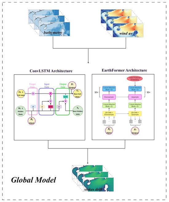
Figure 1.
Deep learning model schematic diagram.
Earthformer employs a cuboid attention mechanism for spatiotemporal sequence prediction [38]. It divides the input tensor into non-overlapping cuboids, applies self-attention within each block, and merges the results using global vectors to facilitate inter-cuboid communication. This streamlined approach, following the decompose–attend–merge process, has shown superior performance over models like ConvLSTM.
In our experiments, all data were first normalized before being fed into the ConvLSTM and Earthformer models to mitigate scale differences between features. Specifically, we utilized 36 h of wind speed and water depth data as inputs to predict the subsequent 36 h of Stokes drift. We set the batch size to 32 and trained the model for 50 epochs, employing an early-stopping mechanism with a patience of 30 epochs to prevent overfitting. For optimization, we used the Adam optimizer with a specified learning rate and a weight decay of 1 × 10⁻⁵ to enhance generalization. To further stabilize the training process, we implemented a cosine annealing learning rate scheduler, which dynamically adjusted the learning rate throughout training. Moreover, in our experiments, we defined the loss function by minimizing the mean squared error (MSE).
2.3. Experimental Design
In addition to the wind velocity which is typically used in the estimation and prediction of surface waves and Stokes drift [39,40,41,42], Stokes drift also depends on water depth, particularly in shallow water [14,27]. Therefore, we chose wind velocity and water depth as the input variables for the deep learning models to predict Stokes drift.
We designed three sets of experiments, which were distinguished by their training objectives (Table 1). Namely, the input variables were the same (wind velocity components u and v and water depth h) in the three experiments; however, the training objectives were different.

Table 1.
Experimental inputs and training objectives.
The loss functions (Equations (1)–(3)) for each experiment were as follows:
where denotes the reanalysis data (“truth”), and refers to the predictions from the deep learning model.
3. Results
3.1. Earthformer
We predicted a yearlong surface Stokes drift using the deep learning model. The 1-year averaged Stokes drift demonstrated that Exp. 1 exhibited larger errors in Stokes drift direction compared to Exp. 2 and Exp. 3 (Figure 2). By contrast, Exp. 2 and Exp. 3 showed an overall high consistency with CMEMS reanalysis data in terms of both Stokes drift magnitude and direction. Particularly, by explicitly considering both the magnitude and direction information of Stokes drift, Exp. 3 was able to capture its characteristics better, improving the prediction accuracy.
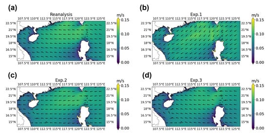
Figure 2.
Surface Stokes drift from (a) CMEMS reanalysis data and (b,c) Earthformer predictions from (b) Exp. 1, (c) Exp. 2, and (d) Exp. 3. The results are temporally averaged over a year. The background color denotes the magnitude of Stokes drift. The magnitude is computed as and the direction is determined by arctan2 (vs, us).
As shown in Figure 3a, Exp. 1 performed well only in predicting the Stokes drift magnitude during certain months. However, significant discrepancies were observed between the model predictions and the reanalysis data. Exp. 1 exhibited larger errors in predicting the Stokes drift magnitude across the entire region (Figure 3d) than Exp. 2 and Exp. 3 (Figure 3e,f). Additionally, Exp. 1 showed low accuracy in predicting the Stokes drift direction (Figure 4a), with notable errors observed in certain months. The regional distribution map further highlighted significantly larger errors in coastal areas (Figure 4d).
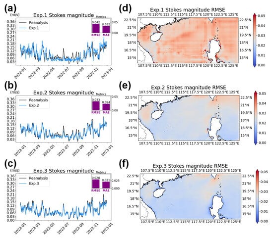
Figure 3.
Earthformer predictions of (left column) surface Stokes drift magnitude and (right column) corresponding RMSE from (top row) Exp. 1, (middle row) Exp. 2, and (bottom row) Exp. 3. The purple bars represent the overall RMSE and MAE.
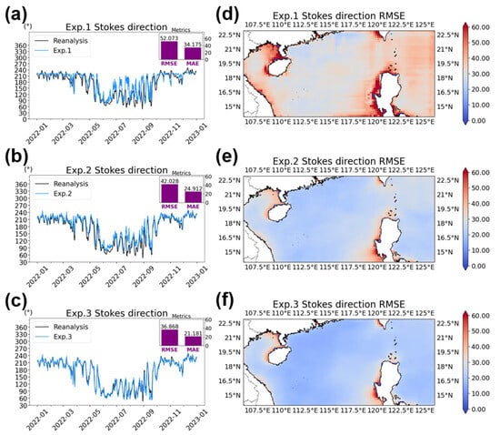
Figure 4.
Earthformer predictions of (left column) surface Stokes drift direction and (right column) corresponding RMSE from (top row) Exp. 1, (middle row) Exp. 2, and (bottom row) Exp. 3. The purple bars represent the overall RMSE and MAE.
Compared to Exp. 1, Exp. 3 reduced the RMSE by 33% for the Stokes drift magnitude prediction (Figure 3a,c) and by 29% for the direction prediction (Figure 4a,c). Additionally, Exp. 3 achieved consistently low RMSE values across the entire region for both Stokes drift magnitude and direction predictions (Figure 3c and Figure 4c), with only minor errors near coastal areas (Figure 3f and Figure 4f), likely due to the significant variability in wave conditions over there [43]. In brief, Exp. 3 outperformed the other two experiments in terms of both Stokes drift magnitude and direction. This suggests that using the magnitude and direction as training objectives is more suitable for Stokes drift prediction.
The above analysis of prediction accuracy was based on the accuracy of Stokes drift magnitude and direction. Furthermore, we assessed the prediction accuracy in terms of the accuracy of Stokes drift components, i.e., the eastward and northward velocity components (us, vs). We decomposed the Exp. 3 training objectives of Stokes drift magnitude and direction θ into Stokes drift components (us, vs), that is, us = cos θ and vs = sin θ.
Again, Exp. 2 and Exp. 3 demonstrated significant improvement over Exp. 1 in predicting Stokes drift components (us, vs). Particularly, the RMSE in Exp. 3 for the predicted Stokes drift components us and vs was reduced by approximately 22% and 31% compared to Exp. 1 (Figure 5). This further confirmed that using Stokes drift magnitude and direction as the training objectives (Exp. 3) can significantly improve the accuracy of Stokes drift prediction compared to using Stokes drift components as the training objectives (Exp. 1).
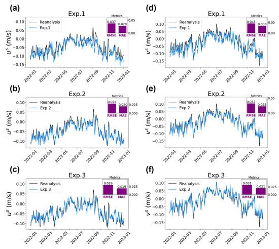
Figure 5.
Time series of spatially averaged surface Stokes drift components (left column) us and (right column) vs from (a,d) Exp. 1, (b,e) Exp. 2, and (c,f) Exp. 3. The purple bars represent the overall RMSE and MAE.
3.2. ConvLSTM
Further, we conducted the same three experiments but using the ConvLSTM model. This was to examine whether the finding that using Stokes drift magnitude and direction as the training objectives is better than using Stokes drift components worked for a different deep learning model other than the Earthformer.
Consistent with the results from the Earthformer model, Exp. 3 demonstrated a significantly improved performance in predicting both the Stokes drift magnitude and direction, with enhancements of 25% and 11%, respectively, compared to Exp. 1 (Figure 6 and Figure 7). However, the improvement in Exp. 2′s results was relatively modest in terms of Stokes drift magnitude (Figure 6b,e). This may be attributed to structural differences between Earthformer and ConvLSTM models, as Earthformer’s global self-attention mechanism appears to better capture changes in magnitude from directional information [44].
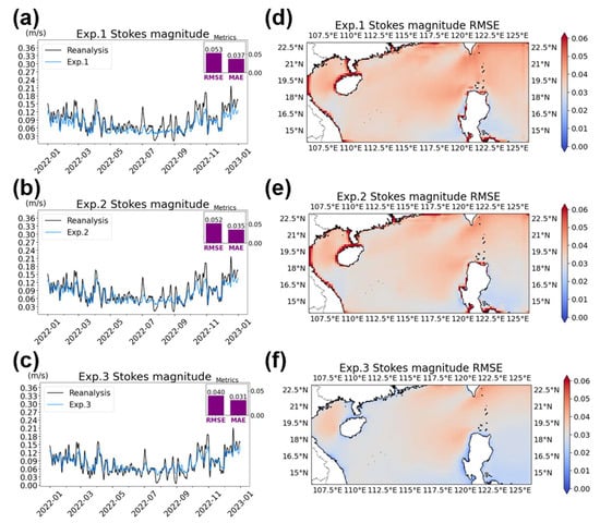
Figure 6.
ConvLSTM predictions of (left column) surface Stokes drift magnitude and (right column) corresponding RMSE from (top row) Exp. 1, (middle row) Exp. 2, and (bottom row) Exp. 3. The purple bars represent the overall RMSE and MAE.
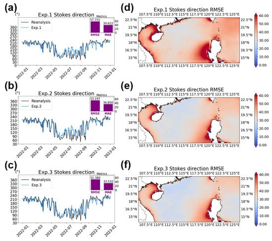
Figure 7.
ConvLSTM predictions of (left column) surface Stokes drift direction and (right column) corresponding RMSE from (top row) Exp. 1, (middle row) Exp. 2, and (bottom row) Exp. 3. The purple bars represent the overall RMSE and MAE.
Further, we calculated the prediction accuracy in terms of the Stokes drift components. Again, Exp. 3 achieved a significant accuracy improvement relative to Exp. 1 (Figure 8a,d). Specifically, the RMSE for the predicted Stokes drift components us and vs in Exp. 3 was reduced by approximately 22% and 31%, respectively, compared to Exp. 1. This confirmed that using Stokes drift magnitude and direction as the training objectives (Exp. 3) can significantly improve the accuracy of Stokes drift prediction compared to using Stokes drift components as the training objectives (Exp. 1). Additionally, Exp. 2 showed only a relatively modest improvement in predicting the Stokes drift components (Figure 8b,e) compared to Exp. 1. This aligns with the results shown in Figure 6b,e, which also indicate relatively modest improvements in Exp. 2.
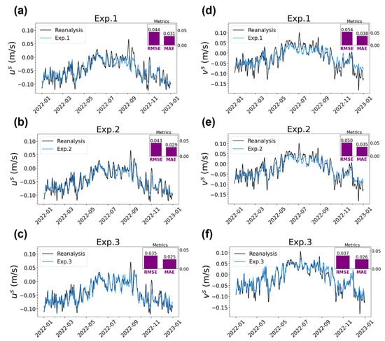
Figure 8.
Time series of spatially averaged surface Stokes drift components (left column) us and (right column) vs, derived from ConvLSTM experiments: (a,d) Exp. 1, (b,e) Exp. 2, and (c,f) Exp. 3. The purple bars represent the overall RMSE and MAE.
3.3. Seasonality and Prediction Duration
In the northern part of the South China Sea, the prediction results for Stokes drift exhibited significant seasonal differentiation (Figure 9). The motivation for this seasonal analysis arose from the unique monsoon climate system and the strong seasonal coupling between multi-scale ocean dynamics in the South China Sea [45]. In the summer, the high-energy wave field driven by the southwest monsoon and the strong shear-dominated flow field under the winter northeast monsoon modulate the spatiotemporal distribution of Stokes drift in distinct ways [46]. In this context, quantifying the seasonal characteristics of prediction errors can reveal the model’s sensitivity and limitations under varying oceanic seasonal conditions.
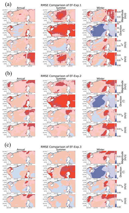
Figure 9.
Spatial RMSE distribution maps predicted by the Earthformer Exp. 3 model using data from the entire year of 2022. From top to bottom, the panels represent magnitude (m/s), direction (°), us (m/s), and vs (m/s), corresponding to (left column) full-year, (middle column) summer, and (right column) winter averages.
For magnitude prediction, the RMSE in the summer was generally higher than the annual average—with peak values reaching 0.04 m/s in deep-water areas—and exhibited a typical spatial pattern of “high in deep water, low nearshore.” In contrast, winter errors were concentrated around the dynamically complex Luzon Strait (RMSE > 0.03 m/s). Notably, Experiment 3 showed significant improvements in high-error regions; for instance, in summer deep-water areas, the magnitude RMSE decreased from 0.04 m/s to 0.02 m/s—a reduction of 50%.
The seasonal differences in directional prediction errors were even more pronounced. During the summer, directional errors were generally high across the entire region, whereas in the winter, the overall error level was lower (with deep-water averages of less than 10°). Exp. 3 reduced the summer deep-water directional error from 60° in Exp. 1 to 20°, corresponding to an improvement of 67%. Although the absolute improvement in the winter was smaller due to the lower baseline error (less than 15°), Exp. 3 still maintained optimal performance. Additionally, the highest prediction errors for the Stokes drift components (us and vs) were primarily located around the Luzon Strait in the winter and in deep-water regions during the summer, where Exp. 3 could improve the component predictions by as much as 0.03 m/s.
Taking the best-performing Earthformer model, Exp. 3, as an example (Figure 10), as the forecast lead time increased, the prediction errors for the magnitude and direction of the Stokes drift exhibited distinct spatiotemporal characteristics. In the first 18 h, the error in magnitude remained relatively small and grew slowly, indicating that the model could capture the variations in the magnitude of the Stokes drift well in short-term forecasts. However, from 18 to 36 h, the error in magnitude increased rapidly, especially in the Luzon Strait and the Beibu Gulf, a phenomenon which might have been related to the complex topographic variations in these areas [47]. Complex topography can alter the propagation path and energy distribution of ocean waves, thereby affecting the magnitude of the Stokes drift, making long-term forecasts require more terrain-related variables as the inputs for the model.
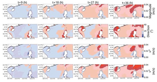
Figure 10.
Spatial RMSE distribution maps predicted by the Earthformer Exp. 3 model using data from the entire year of 2022. From top to bottom, the panels represent magnitude (m/s), direction (°), us (m/s), and vs (m/s); from left to right, they display the average RMSE for the 9th, 18th, 27th, and 36th-hour predictions.
For the prediction of direction, the low error in deep-water regions was maintained at a low level for the first 27 h. However, the error around the Philippine Islands remained relatively high from 9 to 36 h, and the error in coastal areas increased significantly at 36 h. The direction of the Stokes drift is jointly influenced by the wind and wave fields, and in nearshore areas, the combined effects of swell and wind waves may lead to increased uncertainty in directional predictions [48].
Similarly to the magnitude and direction, the errors of the Stokes drift components us and vs increased only slightly during the first 18 h but then increased significantly in the subsequent 18 h, especially in the Luzon Strait region. Overall, while the model was able to capture the changes in the magnitude and direction of the Stokes drift well in short-term forecasts, the interactions between complex topography, wind fields, and wave fields significantly increased the prediction error in long-term forecasts.
3.4. Performance Evaluation
The Earthformer model Exp. 3 demonstrated excellent performance in predicting the Stokes drift. As the forecast lead time increased, the prediction error (RMSE) showed a slight upward trend. At a t + 3 h forecast, the model achieved an RMSE of 0.019 m and a coefficient of determination (R2) of 0.90 (Figure 11), indicating a high level of agreement between the predicted and observed values. As the forecast lead time extended to t + 36 h, the RMSE increased slightly to 0.033 m, and the R2 dropped to 0.70. The scatter plot showed that the data points were well aligned with the 1:1 line, and the least-squares regression (LSR) line was close to the 1:1 line.
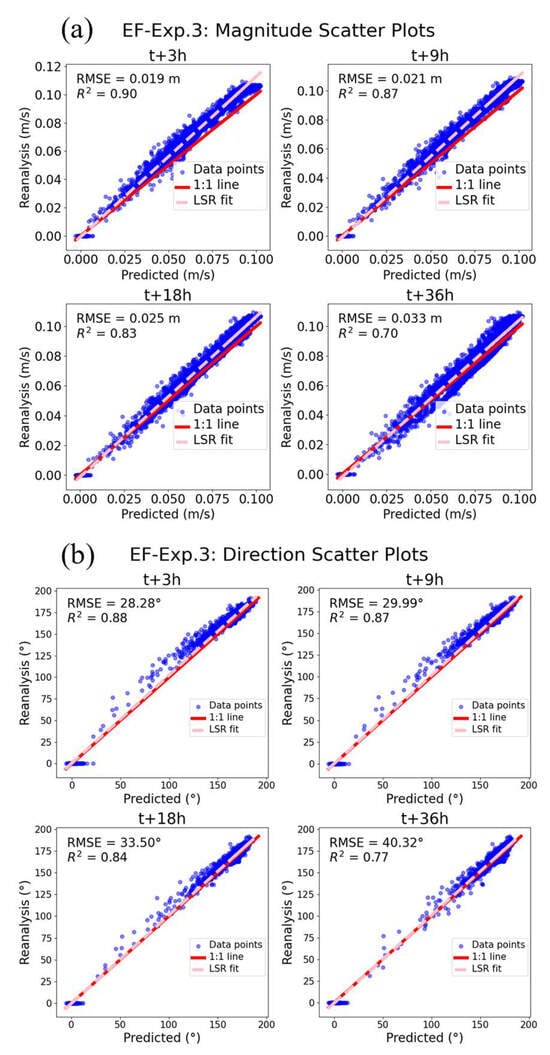
Figure 11.
Magnitude and direction scatter plots for EF-Exp. 3 at different lead times. Blue dots represent data points, the red line indicates the 1:1 line, and the pink line shows the LSR fit.
In terms of direction prediction (Figure 11b), the data points averaged over the entire year were mainly concentrated in the 150°–200° range. At a t + 3 h forecast, the RMSE was 29.99°, and the R2 was 0.93, while at the longer t + 36 h forecast, the RMSE increased to 40.32°, and the R2 dropped to 0.88. These results indicated that the deep learning model for predicting Stokes drift based on wind speed and water depth was feasible [49]. Short-term forecasts exhibited consistently high performance in terms of RMSE and R2, and although the long-term predictions showed some decline, they remained within acceptable limits. Moreover, the model that used magnitude and direction as the training objectives further enhanced the prediction performance compared to directly using the components. In the future, incorporating additional variables is expected to further improve the long-term forecast accuracy.
4. Discussion
Accurately predicting surface Stokes drift is crucial for understanding and modeling ocean dynamics, particularly in material transport, mixed-layer dynamics, and pollutant dispersion. This study employed advanced deep learning models, Earthformer and ConvLSTM, to explore the impact of different training objectives on the prediction accuracy. The discussion will be structured around four key aspects: the dynamic causes of seasonal prediction errors (Section 4.1), the advantages of model architecture (Section 4.2), and the predictability of oceanic processes (Section 4.3).
4.1. Dynamic Causes of Seasonal Prediction Errors
The seasonal differences in Stokes drift prediction errors in the South China Sea originate from the complex interactions between the East Asian monsoon system and regional ocean dynamics [50]. In the summer, under the dominance of the southwest monsoon, the wave energy spectrum in the South China Sea significantly shifts toward high frequencies, making Stokes drift highly sensitive to wave shape asymmetry, directly leading to a significant increase in prediction errors in deep-water regions [51]. The root mean square error (RMSE) of magnitude prediction in the summer increases by more than 50% compared to the winter, while direction prediction errors even reach three times those in the winter (Figure 9). In contrast, during the winter period dominated by the northeast monsoon, the strong shear flow field in the Luzon Strait and its interaction with complex topography significantly enhance wave refraction effects, causing prediction errors to concentrate in this region (with the magnitude RMSE exceeding 0.03 m/s) [52]. Exp. 3, by explicitly incorporating both drift magnitude and direction into the training objectives, effectively reduced cumulative errors in high-error regions, particularly in deep-water areas during the summer, where the RMSE of the drift direction decreased significantly from 60° to 20°. Due to the optimization of the training objectives, the model effectively learnt the nonlinear phase–amplitude interactions of the wave field, enhancing its ability to capture dynamic wave field characteristics.
4.2. Advantages of Model Architecture
The deep learning model Earthformer demonstrated significant predictive advantages over ConvLSTM, particularly excelling in long-term sequence forecasting. This performance difference fundamentally arose from Earthformer’s transformer architecture, which, through a global self-attention mechanism, effectively captured long-range spatial correlations and complex monsoon-scale interactions between wave fields, wind fields, and current fields [38]. In contrast, the ConvLSTM model relied on a local convolution-based spatial information capture strategy [37], limiting its ability to perceive large-scale wave propagation and dynamic interaction processes.
4.3. Predictability of Ocean Dynamic Processes
The Earthformer model maintained a stable high-accuracy performance in short-term forecasts within 0–18 h. However, in the 18–36 h range, prediction errors rapidly increased (Figure 11), especially in topographically complex regions such as the Luzon Strait and the Beibu Gulf (Figure 10). This phenomenon resulted from the amplification effect of nonlinear interactions between wave propagation paths and complex topography as the prediction lead time increased [53]. Despite this error growth trend, the Earthformer model still exhibited a significantly better generalization capability than ConvLSTM in the 36 h forecast range. However, in long-term prediction scenarios, the complex superposition effects of nearshore wave fields significantly increased model prediction uncertainty. Future research should focus on modeling the dynamic mechanisms of complex topographic regions and optimizing training strategies to further enhance the model’s long-term forecasting capability.
5. Conclusions
In this study, we employed two deep learning models, i.e., Earthformer and ConvLSTM, to predict surface Stokes drift and designed three experiments distinguished by their training objectives (Table 1). The prediction accuracy of Stokes drift was measured in terms of two criteria: (1) the Stokes drift magnitude and direction and (2) the two Stokes drift components. Both Earthformer and ConvLSTM achieved the best results in Exp. 3 for predicting Stokes drift magnitude, direction, and components (us, vs). In other words, using Stokes drift magnitude and direction as the training objectives markedly enhanced the prediction accuracy of Stokes drift compared to using its components. Particularly, the RMSE was reduced by 30% for magnitude prediction and 28% for direction prediction, as well as 22% and 31% for Stokes drift components (us, vs). Additionally, in Exp. 3, the Earthformer model demonstrated a significant improvement over the ConvLSTM model. Moreover, this method of using magnitude and direction as the training objectives can also be used for predicting other vector variables, such as ocean currents and winds. In 1 h forecasts, this model was capable of controlling the root mean square error of each component of the Stokes drift between 0.019 and 0.021 m/s. Although the error increased with longer forecast times, the overall average error remained around 0.03 m/s.
However, this study did not take into account other environmental variables as inputs, such as ocean currents and sea surface height, which can affect the evolution of surface waves and thereby the Stokes drift. Exploring these additional variables in future research could provide further insights into enhancing the accuracy of Stokes drift prediction using deep learning models. Future improvements could focus on optimizing input variable selection, enhancing the resolution of reanalysis data, and exploring additional advanced neural network architectures to enhance predictive performance.
This study primarily focused on the Stokes drift and did not encompass all sea surface flow mechanisms. We acknowledge that considering only the Stokes drift does not fully capture the complexities of sea surface transport, as other processes (such as Ekman currents, Langmuir circulation, and breaking waves) may also play significant roles under varying sea conditions and wind fields. However, current research on these processes still faces considerable challenges in large-scale or long-term observational and modeling efforts: for instance, Langmuir circulation typically requires high-resolution large eddy simulations and high-precision air–sea coupled observations for accurate characterization, while the process of breaking waves is often dominated by instantaneous, localized turbulence, and existing operational wave models provide only a relatively coarse description that is insufficient for accurate large-scale quantitative assessments. We look forward to continuous advances in observational and numerical simulation technologies, which will eventually enable the more accurate incorporation of these additional processes into sea surface flow studies.
Supplementary Materials
The following supporting information can be downloaded at: https://www.mdpi.com/article/10.3390/w17070983/s1, Figure S1: Validation of Stokes drift; Figure S2: Sensitivity experiments on Random noise; Figure S3: Sensitivity experiments on Training duration. Reference [54] is cited in the Supplementary Materials.
Author Contributions
Conceptualization, D.L.Y. and P.W.; data curation, X.Y.; formal analysis, X.Y.; funding acquisition, P.W.; investigation, X.Y.; project administration, P.W.; resources, P.W.; supervision, P.W.; visualization, X.Y.; writing—original draft, X.Y.; and writing—review and editing, D.L.Y. and P.W. All authors have read and agreed to the published version of the manuscript.
Funding
This research was funded by the National Key Research and Development Program of China (grant no. 2024YFC3013200 and 2023YFC3008200), the Natural Science Foundation of the Guangdong Province (grant no. 2022A1515110914), and the National Natural Science Foundation of China (grant no. 42206017 and 42306011).
Data Availability Statement
The wind velocity and surface Stokes drift velocity data were obtained from the Copernicus Marine Environment Monitoring Service (CMEMS) at https://resources.marine.copernicus.eu/products (accessed on 10 March 2024), and the depth data were sourced from the ETOPO Global Relief Model available at https://www.ncei.noaa.gov/products/etopo-global-relief-model (accessed on 25 March 2024).
Acknowledgments
We would like to express our sincere gratitude to the Editor and two anonymous reviewers for their valuable comments and suggestions.
Conflicts of Interest
The authors declare that they have no known competing financial interests or personal relationships that could have appeared to influence the work reported in this paper.
References
- Stokes, G.G. On the theory of oscillatory waves. Trans. Camb. Philos. Soc. 1847, 8, 441–455. [Google Scholar]
- van den Bremer, T.S.; Breivik, Ø. Stokes drift. Philos. Trans. R. Soc. A Math. Phys. Eng. Sci. 2017, 376, 20170104. [Google Scholar] [CrossRef]
- Webber, J.J.; Huppert, H.E. Stokes drift in coral reefs with depth-varying permeability. Philos. Trans. R. Soc. A Math. Phys. Eng. Sci. 2020, 378, 20190531. [Google Scholar] [CrossRef]
- Franks, P.J.S.; Garwood, J.C.; Ouimet, M.; Cortes, J.; Musgrave, R.C.; Lucas, A.J. Stokes drift of plankton in linear internal waves: Cross-shore transport of neutrally buoyant and depth-keeping organisms. Limnol. Oceanogr. 2019, 65, 1286–1296. [Google Scholar] [CrossRef]
- Rascle, N.; Ardhuin, F.; Queffeulou, P.; Croizé-Fillon, D. A global wave parameter database for geophysical applications. Part 1: Wave-current–turbulence interaction parameters for the open ocean based on traditional parameterizations. Ocean Modell. 2008, 25, 154–171. [Google Scholar] [CrossRef]
- Yadav, A.; Kumar, P.; Bhaskaran, P.K.; Hisaki, Y. Evaluation of ocean wave power utilizing COWCLIP 2.0 datasets: A CMIP5 model assessment. Clim. Dyn. 2024, 62, 9447–9468. [Google Scholar] [CrossRef]
- Zhang, X.; Wang, Z.; Wang, B.; Wu, K.; Han, G.; Li, W. A numerical estimation of the impact of Stokes drift on upper ocean temperature. Acta Oceanol. Sin. 2014, 33, 48–55. [Google Scholar] [CrossRef]
- Bosi, S.; Broström, G.; Roquet, F. The role of Stokes drift in the dispersal of North Atlantic surface marine debris. Front. Mar. Sci. 2021, 8, 697430. [Google Scholar] [CrossRef]
- Heath, N. Determining the Effects of Stokes Drift on the Movement of Oil in the Gulf of Mexico. Ph.D. Dissertation, Florida State University, Tallahassee, FL, USA, 2011. Environmental Science, Geology. Available online: https://api.semanticscholar.org/CorpusID:29983443 (accessed on 10 March 2024).
- Yang, Y.; Li, Y.; Li, J.; Liu, J.; Gao, Z.; Guo, K.; Yu, H. The influence of Stokes drift on oil spills: Sanchi oil spill case. Acta Oceanol. Sin. 2021, 40, 30–37. [Google Scholar] [CrossRef]
- Sutherland, G.; Soontiens, N.; Davidson, F.; Smith, G.C.; Bernier, N.; Blanken, H.; Schillinger, D.; Marcotte, G.; Röhrs, J.; Dagestad, K.-F.; et al. Evaluating the leeway coefficient of ocean drifters using operational marine environmental prediction systems. J. Atmos. Ocean. Technol. 2020, 37, 1943–1954. [Google Scholar] [CrossRef]
- Mediavilla, D.; Sepúlveda, H.H.; Alonso, G. Wind and wave height climate from two decades of altimeter records on the Chilean Coast (15°–56.5°S). Ocean Dyn. 2020, 70, 231–239. [Google Scholar] [CrossRef]
- Zimmerman, J.T.F. On the Euler-Lagrange transformation and the Stokes' drift in the presence of oscillatory and residual currents. Deep Sea Res. A Oceanogr. Res. Pap. 1979, 26, 505–520. [Google Scholar] [CrossRef]
- McWilliams, J.C.; Restrepo, J.M.; Lane, E.M. An asymptotic theory for the interaction of waves and currents in coastal waters. J. Fluid Mech. 2004, 511, 135–178. [Google Scholar] [CrossRef]
- Wang, P.; McWilliams, J.C.; Wang, D.; Li Yi, D. Conservative Surface Wave Effects on a Wind-Driven Coastal Upwelling System. J. Phys. Oceanogr. 2022, 53, 37–55. [Google Scholar] [CrossRef]
- Wang, P.; McWilliams, J.C.; Uchiyama, Y.; Chekroun, M.D.; Li Yi, D. Effects of Wave Streaming and Wave Variations on Nearshore Wave-Driven Circulation. J. Phys. Oceanogr. 2020, 50, 3025–3041. [Google Scholar] [CrossRef]
- Ardhuin, F.; Chapron, B.; Elfouhaily, T. Waves and the air–sea momentum budget: Implications for ocean circulation modeling. J. Phys. Oceanogr. 2004, 34, 1741–1755. [Google Scholar] [CrossRef]
- Henry, D. Stokes drift in equatorial water waves, and wave–current interactions. Deep Sea Res. II Top. Stud. Oceanogr. 2019, 160, 41–47. [Google Scholar] [CrossRef]
- Large, W.G.; Patton, E.G.; DuVivier, A.K.; Sullivan, P.P.; Romero, L. Similarity theory in the surface layer of large-eddy simulations of the wind-, wave-, and buoyancy-forced Southern Ocean. J. Phys. Oceanogr. 2019, 49, 2165–2187. [Google Scholar] [CrossRef]
- Tamura, H.; Miyazawa, Y.; Oey, L.-Y. The Stokes drift and wave-induced mass flux in the North Pacific. J. Geophys. Res. Oceans 2012, 117, C8. [Google Scholar] [CrossRef]
- Kantha, L.H.; Clayson, C.A. On the effect of surface gravity waves on mixing in the oceanic mixed layer. Ocean Modell. 2004, 6, 101–124. [Google Scholar] [CrossRef]
- Craik, A.D.D.; Leibovich, S. A rational model for Langmuir circulations. J. Fluid Mech. 1976, 73, 401–426. [Google Scholar] [CrossRef]
- McWilliams, J.C.; Sullivan, P.P.; Moeng, C.-H. Langmuir turbulence in the ocean. J. Fluid. Mech. 1997, 334, 1–30. [Google Scholar] [CrossRef]
- Wang, P.; Özgökmen, T.M. Langmuir circulation with explicit surface waves from moving-mesh modeling. Geophys. Res. Lett. 2018, 45, 216–226. [Google Scholar] [CrossRef]
- Longuet-Higgins, M.S. Mass transport in water waves. Philos. Trans. R. Soc. Lond. A 1953, 245, 535–581. [Google Scholar] [CrossRef]
- Ursell, F. Surface waves on deep water in the presence of a submerged circular cylinder. Math. Proc. Camb. Philos. Soc. 1950, 46, 141–152. [Google Scholar] [CrossRef]
- Kenyon, K.E. Stokes Drift for Random Gravity Waves. J. Geophys. Res. 1969, 74, 6991–6994. [Google Scholar] [CrossRef]
- Webb, A.; Fox-Kemper, B. Impacts of wave spreading and multidirectional waves on estimating Stokes drift. Ocean Modell. 2015, 96, 49–64. [Google Scholar] [CrossRef]
- Chen, J.; Gong, X.; Guo, X.; Xing, X.; Lu, K.; Gao, H.; Gong, X. Improved perceptron of subsurface chlorophyll maxima by a deep neural network: A case study with BGC-Argo float data in the northwestern Pacific Ocean. Remote Sens. 2022, 14, 632. [Google Scholar] [CrossRef]
- Krishna Kumar, N.; Savitha, R.; Al Mamun, A. Regional ocean wave height prediction using sequential learning neural networks. Ocean Eng. 2017, 129, 605–612. [Google Scholar] [CrossRef]
- Liu, Y.; Lu, W.; Wang, D.; Lai, Z.; Ying, C.; Li, X.; Han, Y.; Wang, Z.; Dong, C. Spatio-temporal wave forecast with transformer-based network: A case study for the northwestern Pacific Ocean. Ocean Modell. 2024, 188, 102323. [Google Scholar] [CrossRef]
- Mandal, S.; Prabaharan, N. Ocean wave forecasting using recurrent neural networks. Ocean Eng. 2006, 33, 1401–1410. [Google Scholar] [CrossRef]
- Miao, Y.; Zhang, X.; Li, Y.; Lianxin, Z.; Zhang, D. Monthly extended ocean predictions based on a convolutional neural network via the transfer learning method. Front. Mar. Sci. 2023, 9, 1073377. [Google Scholar] [CrossRef]
- Song, Y.; Jiang, H. A deep learning–based approach for empirical modeling of single-point wave spectra in open oceans. J. Phys. Oceanogr. 2023, 53, 2089–2103. [Google Scholar] [CrossRef]
- Wang, C.; Zheng, G.; Li, X.; Liu, B.; Xu, Q.; Zhang, J. Tropical cyclone intensity estimation from geostationary satellite imagery using deep convolutional neural networks. IEEE Trans. Geosci. Remote Sens. 2022, 60, 4101416. [Google Scholar] [CrossRef]
- Liu, G.; Perrie, W.; He, Y. Ocean surface Stokes drift from scatterometer observations. Int. J. Remote Sens. 2014, 35, 1966–1978. [Google Scholar] [CrossRef]
- Shi, X.; Chen, Z.; Wang, H.; Yeung, D.-Y.; Wong, W.-K.; Woo, W.-C. Convolutional LSTM network: A machine learning approach for precipitation nowcasting. arXiv 2015. [Google Scholar] [CrossRef]
- Gao, Z.; Shi, X.; Wang, H.; Zhu, Y.; Wang, Y.B.; Li, M.; Yeung, D.-Y. Earthformer: Exploring space-time transformers for earth system forecasting. arXiv 2022. [Google Scholar] [CrossRef]
- Chalikov, D. Numerical modeling of surface wave development under the action of wind. Ocean Sci. 2018, 14, 453–470. [Google Scholar] [CrossRef]
- Lenain, L.; Pizzo, N. The contribution of high-frequency wind-generated surface waves to the Stokes drift. J. Phys. Oceanogr. 2020, 50, 3455–3465. [Google Scholar] [CrossRef]
- Tamtare, T.; Dumont, D.; Chavanne, C. The Stokes drift in ocean surface drift prediction. J. Oper. Oceanogr. 2021, 15, 156–168. [Google Scholar] [CrossRef]
- Zamani, A.; Solomatine, D.; Azimian, A.; Heemink, A. Learning from data for wind–wave forecasting. Ocean Eng. 2008, 35, 953–962. [Google Scholar] [CrossRef]
- Su, J. Overview of the South China Sea circulation and its influence on the coastal physical oceanography outside the Pearl River Estuary. Cont. Shelf Res. 2004, 24, 1745–1760. [Google Scholar] [CrossRef]
- Ge, K.; Wang, C.; Guo, Y.-T.; Tang, Y.-S.; Fan, J.-S. A Multitask Fourier Transformer Network for Seismic Source Characterization Estimation From a Single-Station Waveform. IEEE Geosci. Remote Sens. Lett. 2024, 21, 7503805. [Google Scholar] [CrossRef]
- Hu, P.; Chen, W.; Chen, S.; Wang, L.; Huang, R. Impact of the March Arctic Oscillation on the South China Sea summer monsoon onset. Int. J. Climatol. 2020, 41, E3239–E3248. [Google Scholar] [CrossRef]
- Wang, Z.; Duan, C.; Dong, S. Long-term wind and wave energy resource assessment in the South China Sea based on 30-year hindcast data. Ocean Eng. 2018, 163, 58–75. [Google Scholar] [CrossRef]
- Gao, J.; Wu, G.; Ya, H. Review of the circulation in the Beibu Gulf, South China Sea. Cont. Shelf Res. 2017, 138, 106–119. [Google Scholar] [CrossRef]
- Röhrs, J.; Christensen, K.H.; Hole, L.R.; Broström, G.; Drivdal, M.; Sundby, S. Observation-based evaluation of surface wave effects on currents and trajectory forecasts. Ocean Dyn. 2012, 62, 1519–1533. [Google Scholar] [CrossRef]
- Liu, D.; Li, Y.; Mu, L. Parameterization modeling for wind drift factor in oil spill drift trajectory simulation based on machine learning. Front. Mar. Sci. 2023, 10, 1222347. [Google Scholar] [CrossRef]
- He, Z.; Wu, R. Seasonality of interannual atmosphere–ocean interaction in the South China Sea. J. Oceanogr. 2013, 69, 699–712. [Google Scholar] [CrossRef]
- Bao, Y.; Song, Z.; Qiao, F. FIO-ESM Version 2.0: Model Description and Evaluation. J. Geophys. Res. Ocean. 2020, 125, e2019JC016036. [Google Scholar] [CrossRef]
- Han, W.; Moore, A.M.; Levin, J.; Zhang, B.; Arango, H.G.; Curchitser, E.; Di Lorenzo, E.; Gordon, A.L.; Lin, J. Seasonal surface ocean circulation and dynamics in the Philippine Archipelago region during 2004–2008. Dyn. Atmos. Oceans 2009, 47, 114–137. [Google Scholar] [CrossRef]
- Li, Y.; Xu, Z.; Lv, X. The Generation and Propagation of Wind- and Tide-Induced Near-Inertial Waves in the Ocean. J. Mar. Sci. Eng. 2024, 12, 1565. [Google Scholar] [CrossRef]
- Thomson, J.; D’Asaro, E.A.; Cronin, M.F.; Rogers, W.E.; Harcourt, R.R.; Shcherbina, A. Waves and the equilibrium range at ocean weather station p. J. Geophys. Res. Oceans. 2013, 118, 5951–5962. [Google Scholar] [CrossRef]
Disclaimer/Publisher’s Note: The statements, opinions and data contained in all publications are solely those of the individual author(s) and contributor(s) and not of MDPI and/or the editor(s). MDPI and/or the editor(s) disclaim responsibility for any injury to people or property resulting from any ideas, methods, instructions or products referred to in the content. |
© 2025 by the authors. Licensee MDPI, Basel, Switzerland. This article is an open access article distributed under the terms and conditions of the Creative Commons Attribution (CC BY) license (https://creativecommons.org/licenses/by/4.0/).