Preliminary Multi-Objective Optimization of Mobile Drip Irrigation System Design and Deficit Irrigation Schedule: A Full Growth Cycle Simulation for Alfalfa Using HYDRUS-2D

Abstract

Mobile drip irrigation (MDI) systems integrate the technological advantages of center-pivot irrigation (CPI) systems and drip irrigation systems, boasting a high water-saving potential. To further enhance water use efficiency in alfalfa production in northern China, this preliminary study verified the accuracy of the HYDRUS-2D soil water movement numerical model through field experiments. Using the numerical model, four drip-line installation distances (60, 75, 90, and 105 cm), three deficit irrigation thresholds (45–50% FC, 55–60% FC, and 65–70% FC), and four irrigation depths (70% W, 85% W, 100% W, and 115% W) were set to simulate root water uptake, soil surface evaporation, total irrigation amount, and deep percolation during the entire growth cycle of alfalfa, respectively. Objective functions were constructed according to the simulation results, and the NSGA-II algorithm was used for multi-objective optimization of the deficit irrigation schedule. The preliminary results indicated that HYDRUS-2D can accurately simulate soil water movement under MDI systems, as the RMSE values of soil water content at all measured depths were less than 0.021 cm³/cm³, with the NRMSE values being below 23.3%, and the MAE values below 0.014 cm³/cm³. Increasing the deficit irrigation threshold from F1 to F3 enhanced root water uptake by 12.24–15.34% but simultaneously increased the total irrigation amount, soil surface evaporation (by up to 29.58%), and the risk of deep percolation; similar trends were observed with increasing irrigation depth. The drip-line installation distance had no significant impact on irrigation performance. The NSGA-II multi-objective optimization algorithm was used to obtain Pareto-optimal solutions that balance conflicting objectives. For this case study, a drip-line installation distance of 105 cm, a deficit irrigation threshold of 50–55% FC, and an irrigation depth of 112% W were recommended to achieve balance among the various optimization objectives. This study provides a preliminary framework for optimizing MDI systems and irrigation strategies. However, since a deeper root distribution (>80 cm) was not investigated in this study, future research incorporating deeper root zones is required for developing more comprehensive irrigation scheduling suitable for typical alfalfa cultivation scenarios.

1. Introduction

Given the challenges of climate change and frequent extreme weather events, the conflict between ensuring food security and addressing water scarcity has worsened globally [1,2,3]. Improving agricultural water use efficiency while maintaining crop yields and promoting sustainable agricultural development is key to addressing global food security and water scarcity challenges. Recently, scholars conducted extensive research on efficient water management for crops and water-saving irrigation equipment, leading to advancements in deficit irrigation strategies and precision irrigation technologies.

Deficit irrigation is an effective water-saving irrigation strategy that intentionally supplies less water than the crop’s potential evapotranspiration (ET_p) [4] while sustaining crop productivity and enhancing water use efficiency [5]. Alfalfa is the perennial forage with the largest cultivated area globally [6], playing a significant role in developing the livestock industry in northern China. Due to its long growing season and deep, dense root system, alfalfa has a relatively high water consumption [7,8]. However, its extensive root system enhances its drought tolerance, making it well suited for deficit irrigation. Studies have shown that mild deficit irrigation (70% of full irrigation) has minimal impact on alfalfa yield and nitrogen use efficiency [6] while improving irrigation water productivity [9,10]. Despite its strong adaptability to water conditions, the yield of alfalfa is sensitive to severe water stress [11]. Balancing reduced irrigation water with minimal loss in alfalfa yield is crucial in formulating deficit irrigation schedules.

As a novel water-saving irrigation technology, mobile drip irrigation (MDI) systems replace low-pressure sprinklers on center-pivot irrigation (CPI) systems with high-flowrate pressure-compensating drip lines. This system uses the self-propelled feature of CPI, with drip lines being attached to the CPI main water-conveying pipeline, achieving large-area, low-cost automated irrigation. MDI systems combine the advantages of CPI systems and drip irrigation systems. These systems feature high automation, strong adaptability to terrain, and low operation and maintenance costs while also avoiding crop canopy interception, evaporation and drift losses, and interference with farm machinery operations [12]. MDI systems retain the localized irrigation characteristics of drip irrigation, wetting only part of the soil surface during irrigation [13]. This reduces soil surface evaporation by 35% [14] and prevents water accumulation and slippage in CPI wheel tracks [15]. Consequently, MDI systems achieve higher water use efficiencies than sprinkler irrigation systems [16,17]. Field experiments have shown that MDI systems can achieve 95% water use efficiency in silage maize and alfalfa production. They could also reduce irrigation water by 5–55% in some years while maintaining yield and quality [18], highlighting their significant water-saving potential.

Recently, with advancements in numerical simulations of soil water movement and multi-objective optimization methods, scholars have attempted to combine numerical models with multi-objective optimization algorithms to optimize irrigation system design and irrigation schedule formulation [19,20,21]. However, studies on MDI systems are still limited. A key research focus is determining how to fully harness their water-saving potential in alfalfa production in northern China. Optimizing deficit irrigation schedules to maximize alfalfa yield while minimizing irrigation water consumption remains a critical challenge for scholars. To address these challenges, this preliminary study conducted a one-year field experiment to validate HYDRUS-2D. The validated model was then used to simulate root water uptake, soil surface evaporation, total irrigation amount, and deep percolation throughout the alfalfa growth cycle. Simulations were conducted under different irrigation conditions, considering four drip-line installation distances (60, 75, 90, and 105 cm), three deficit irrigation thresholds (45–50% FC, 55–60% FC, and 65–70% FC), and four irrigation depths (70% W, 85% W, 100% W, and 115% W). Using the NSGA-II multi-objective optimization algorithm, Pareto optimization was conducted on the drip-line installation distance, deficit irrigation threshold, and irrigation depth of the MDI system, aiming to provide insights for optimizing MDI system application in alfalfa production.

2. Materials and Methods

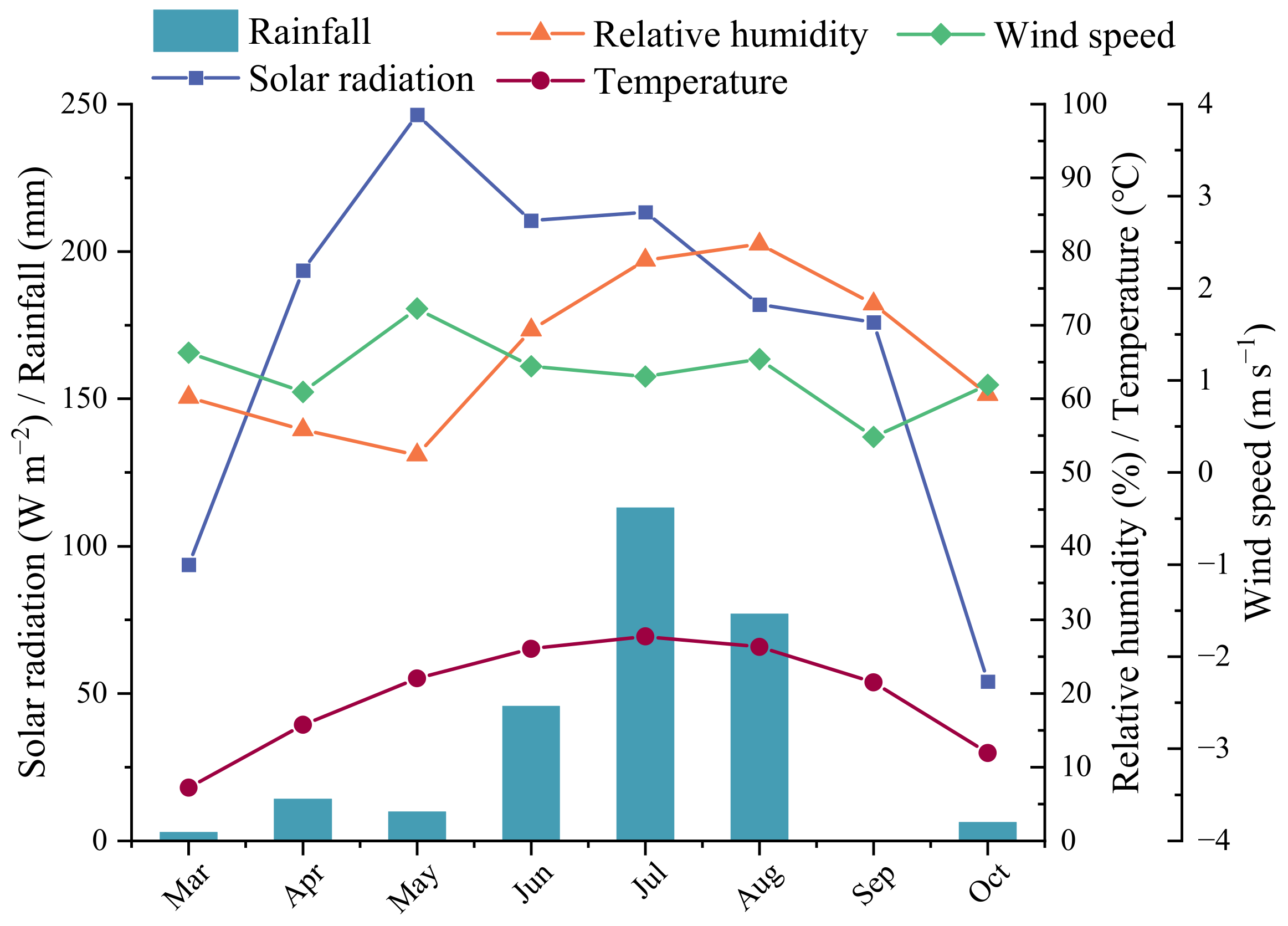
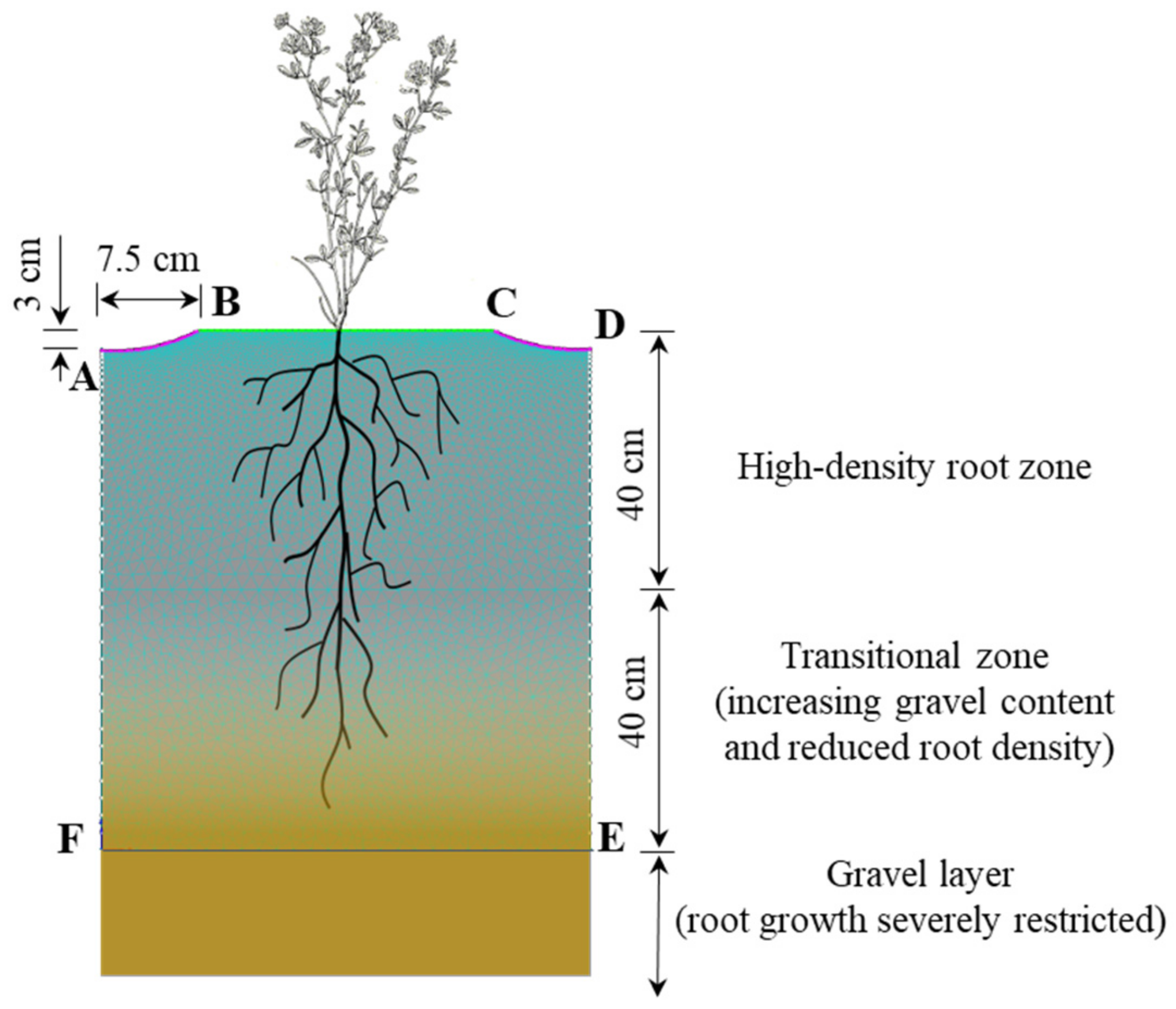
2.1. Field Experiment

In 2022, an alfalfa MDI deficit irrigation experiment was conducted at the China Agricultural University Experimental Station in Zhuozhou (39°27′ N, 115°51′ E) to validate the accuracy of HYDRUS-2D. A CPI system with three spans and one overhang was installed in the field, with the first span modified into the MDI system. The experimental area was located in the first span. The first span of the CPI system was 37 m long, with a drip-line installation distance of 75 cm. The drip-line’s emitters were spaced 15 cm apart, with each discharging at 7.6 L/h. The crop planted was alfalfa in its third year, with a row spacing of 30 cm. The highest root density of alfalfa was observed around 40 cm depth. Below this depth, root distribution was limited due to the increasing presence of gravel. The maximum rooting depth observed was approximately 80 cm, as the gravel layer present below this depth in the experimental field further constrained root development. The local soil type was sandy loam, with a field capacity (FC) of 0.226 cm³/cm³. The soil particle size distribution was determined using an MS2000 laser particle size analyzer (Malvern, UK; measurement error < ±1%, bias < ±0.5%), and the particle size composition was 7.28% for the 0.01–2.00 μm range, 35.07% for the 2.00–50.00 μm range, and 57.65% for the 50.00–2000.00 μm range. The experiment began on March 20th at the beginning of alfalfa regrowth and included four harvests on 23 May, 30 June, 17 August, and 4 October, with a total growth period of 199 days. During this period, the soil volumetric water content at depths of 0–20 cm, 20–40 cm, 40–60 cm, and 60–80 cm was measured twice a week using a TDR Trime-tube system (Trime-T3 TDR, IMKO Ltd., Ettlingen, Baden-Württemberg, Germany). These measured data were subsequently used to validate HYDRUS-2D. Irrigation was triggered when the average soil water content in the planned wetting layer (0–40 cm) dropped to 55–60% FC, and the irrigation amount was determined based on the difference between the average water content at the time of the irrigation initiation and 90% FC. The total rainfall during the entire growth cycle of alfalfa was 254.2 mm, and the total irrigation amount was 308.0 mm.

Meteorological data were collected from a station located approximately 150 m from the experimental site. Figure 1 presents the average monthly rainfall, solar radiation, relative humidity, wind speed, and temperature during the experimental period. These meteorological data were used to calculate the potential evapotranspiration of alfalfa.

2.2. HYDRUS-2D Numerical Model

HYDRUS-2D was used to develop a numerical model of soil water movement under the MDI system for alfalfa. This model was used to investigate soil water dynamics, alfalfa root water uptake, deep percolation, total irrigation amount, and soil surface evaporation throughout the entire growing cycle through the MDI system. The simulation focused on the two-dimensional vertical soil profiles between adjacent mobile drip lines to study soil water movement. As shown in Figure 2, the computational domain in HYDRUS-2D is defined as a rectangle with a width EF equal to the drip-line installation distance (L) and a depth of 80 cm. The mobile drip lines are located at the top-left (A) and top-right corners (B) of the computational domain. Our previous studies [11] indicated that the relative movement of high-flowrate mobile drip lines during irrigation generated localized water accumulation along their paths. This process often resulted in shallow depressions along the soil surface beneath the drip lines, with a maximum depth of approximately 3 cm and a maximum width of approximately 15 cm. To accurately represent this effect, the infiltration boundaries AB and CD were designed as curves. As the crop had a restricted root system due to the presence of a gravel layer at the depth of 80 cm, water leaving the bottom boundary of the computational domain was regarded as deep percolation. The flux across this free drainage boundary was integrated over time to estimate the cumulative deep percolation during the growing cycle.

To optimize the design of the MDI system and the alfalfa deficit irrigation schedule, four drip-line installation distances (L) of 60, 75, 90, and 105 cm were set. Additionally, based on local irrigation practices, three deficit irrigation thresholds were set: 45–50% FC (F1), 55–60% FC (F2), and 65–70% FC (F3). Under each deficit irrigation threshold, four irrigation depths of 70% W (W1), 85% W (W2), 100% W (W3), and 115% W (W4) were set. The irrigation amount (W) was determined based on the difference between the average soil water content in the planned wetting layer at irrigation initiation and 90% FC.

2.2.1. Soil Water Movement Simulation

The soil was assumed to be a homogeneous and isotropic rigid porous medium. Water movement within a two-dimensional soil profile is described using the Richards equation:

$${\displaystyle \frac{\partial \theta }{\partial t}}={\displaystyle \frac{\partial }{\partial x}}\left[K(\theta ){\displaystyle \frac{\partial {\Psi }_m}{\partial x}}\right]+{\displaystyle \frac{\partial }{\partial z}}\left[K(\theta ){\displaystyle \frac{\partial {\Psi }_m}{\partial z}}\right]+{\displaystyle \frac{\partial K(\theta )}{\partial z}}-S(x,z,h)$$

(1)

where x is the horizontal coordinate (cm), z is the vertical coordinate (cm) with the positive direction defined as being vertically upwards, h is the soil water pressure head (cm), θ is the soil volumetric water content (cm³/cm³), t is the numerical simulation time (d), K(θ) is the soil unsaturated hydraulic conductivity (cm/d), Ψ_m is the soil matrix potential (cm), and S(x,z,h) is the sink term describing the crop root water absorption rate (cm³/(cm³·d)).

The strength of soil matrix water retention is related to the soil volumetric water content θ. The relationship between these factors and the soil water characteristic curve are described using the van Genuchten model:

$$S_e={\displaystyle \frac{\theta -{\theta }_r}{{\theta }_s-{\theta }_r}}={\displaystyle \frac{1}{{(1+{\left|\alpha \cdot {\Psi }_m\right|}^n)}^m}}$$

(2)

$$K(S_e)=K_s\cdot S_e^{l^{\prime }}{\left[1-{(1-S_e^{1/m})}^m\right]}^2$$

(3)

where S_e is a dimensionless number representing the effective soil saturation, θ_r is the residual soil water content (cm³/cm³), θ_s is the saturated soil water content (cm³/cm³), K_s is the saturated hydraulic conductivity (cm/d), l’ is the soil pore tortuosity factor, and α, m, and n are dimensionless empirical constants related to the shape of the soil water characteristic curve, with m = 1/n.

The accuracy of numerical simulations with HYDRUS-2D is highly sensitive to soil hydraulic parameters. Therefore, accurately calibrated parameters that reflect actual field soil physical properties are essential. The soil hydraulic parameters of the van Genuchten model used in numerical simulation are shown in

Table 1. The soil hydraulic parameters of the van Genuchten model used in numerical simulation.

θr/ (cm3 cm−3)	θs/ (m3 cm−3)	α/ (cm−1)	n	Ks/ (cm h−1)	l
0.010	0.573	0.003	1.441	2.193	2.734

Notes: θ_r and θ_s represent the residual and the saturated water contents, respectively; K_s denotes the saturated hydraulic conductivity; l′ represents the tortuosity parameter in the conductivity function; and α and n represent shape parameters in the van Genuchten model.

. These parameters were optimized based on preliminary laboratory experiments using soil samples collected from the experimental site. The soil samples were collected in the winter of 2021 from a depth of 0–80 cm. Parameter optimization was conducted through inverse modeling with the built-in inverse solution module of HYDRUS-2D and the Levenberg–Marquardt optimization algorithm.

2.2.2. Crop Evapotranspiration

HYDRUS-2D requires inputting the potential evaporation rate (E_p) and potential transpiration rate (T_p) to simulate water exchange between the soil profile and the atmospheric and root boundaries, ultimately deriving the actual evaporation and transpiration rates.

The potential evapotranspiration of the reference crop (a hypothetical crop with an assumed height of 0.12 m, with a surface resistance of 70 s/m and an albedo of 0.23), closely resembling the evaporation from an extensive surface of green grass of uniform height, actively growing and adequately watered, was calculated using the Penman–Monteith method recommended by FAO [22] based on meteorological data, with the following equation:

$$E{T}_0={\displaystyle \frac{0.408\Delta (R_n-G)+\gamma \frac{900}{T+273}{\mu }_2(e_s-e_a)}{\mathit{\Delta }+\gamma (1+0.34{\mu }_2)}}$$

(4)

where ET₀ is the reference crop evapotranspiration rate (mm/d); R_n is the net radiation (MJ/(m²·d)); G is the soil heat flux (MJ/(m²·d)), taken as zero in this study, with daily calculations; μ₂ is the wind speed at a 2 m height (m/s); e_s is the saturated water vapor pressure (kPa); e_a is the actual water vapor pressure (kPa); Δ is the slope of the saturated water vapor pressure–temperature curve (kPa/°C); γ is the psychrometric constant (kPa/°C); and T is the air temperature (°C).

The dual crop coefficient method from FAO-56 [22] was used to estimate the basal crop coefficient (K_cb) and soil evaporation coefficient (K_e) for each treatment on a daily basis, as well as to calculate the potential evapotranspiration rate, potential transpiration rate, and potential evaporation rate, with the following equations:

$$E{T}_c=(K_{cb}+K_e)E{T}_0$$

(5)

$$T_p=K_{cb}E{T}_0$$

(6)

$$E_p=K_{e}E{T}_0$$

(7)

where ET_c is the potential evapotranspiration (mm/d), K_cb is the basal crop coefficient, K_e is the soil evaporation coefficient, T_p is the potential transpiration rate (mm/d), and E_p is the potential evaporation rate (mm/d).

In numerical simulations, actual evaporation is equal to potential evaporation until the negative pressure head of the surface soil reaches a critical value; at this point, the upper boundary condition is set as a constant head boundary, and soil evaporation is then calculated using Darcy’s law. Since the potential evaporation rate depends on irrigation timing and amount, it must be separately calculated for different deficit irrigation schedules.

2.2.3. Crop Root Water Uptake

Crop root water uptake significantly impacts soil water movement in the root zone. The involvement of roots speeds up the depletion of soil water content in the root zone and reduces the likelihood of deep percolation. Additionally, root water uptake serves as a key reference for optimizing irrigation systems and strategies. In the numerical model, the generalized root water uptake model proposed by Feddes et al. [21] was used to quantify root water uptake per unit time and soil volume, with the following equations:

$$S(x,z,h)=\alpha (x,z,h)\times b(x_1,z_1)\times S_t\times T_p$$

(8)

$$\alpha (h)=\left\{\begin{array}{ll}(h_1-h)/(h_1-h_2)& (h_2<h\le h_1)\\ 1& (h_3\le h<h_2)\\ (h-h_4)/(h_3-h_4)& (h_4\le h<h_3)\end{array}\right.$$

(9)

where x is the horizontal coordinate (cm), z is the vertical coordinate (cm) with a positive direction defined as vertically upwards, and x₁ and z₁ are distances from the origin of the plant in the horizontal and vertical directions, respectively. α(x,z,h) is the dimensionless water stress response function, b(x₁,z₁) is the normalized root water uptake intensity distribution function (cm/cm³), S_t is the soil surface width related to the transpiration process (cm), T_p is the potential transpiration rate in cm/d, h₁ is the value of the pressure head below which the roots start to extract water from the soil (cm), h₂ is the value of the pressure head below which the roots extract water at the maximum possible rate (cm), h₃ is the value of the limiting pressure head below which the roots can no longer extract water at the maximum rate (cm), and h₄ is the value of the pressure head below which root water uptake ceases (cm), usually measured at the wilting point.

The parameters associated with the water stress response function α(x,z,h) for alfalfa are defined in the HYDRUS-2D database, according to the research of Taylor and Ashcroft [23]. The root water uptake intensity distribution function is defined based on the actual root distribution of alfalfa in the field. The alfalfa roots were distributed within a depth of 0–80 cm in the soil profile, with the highest density recorded in the 0–40 cm layer. Below 40 cm, the increasing presence of gravel gradually reduced the root density, and in the model, root water uptake is assumed to occur only within the 0–80 cm soil layer. Given that alfalfa had been established for three years, with small plant spacing and favorable growth conditions, it is reasonable to assume that the root distribution in the soil profile was uniform in the horizontal direction. Thus, based on Vrugt et al. [24], the b(x₁,z₁) function can be simplified into a one-dimensional form as follows:

$$b(x_1,z_1)=b(x_1)=(1-{\displaystyle \frac{z_1}{z_{1m}}})e^{-(p_z\left|z*-z\right|)}$$

(10)

where z_1m is the maximum root distribution depth in the vertical direction (cm), z* is an empirical parameter describing the location of maximum root water uptake in the vertical direction (cm), and P_z is a dimensionless shape parameter that, when z₁ > z*, takes the value of zero.

2.2.4. Initial and Boundary Conditions

As shown in Figure 2, the upper boundaries AB, BC, and CD of the numerical model were defined as atmospheric boundaries, and the boundary conditions were determined from measured meteorological data and the irrigation schedule for potential evaporation estimation. The positions of the mobile drip lines on the upper boundaries (AB and CD) were prescribed considering the latter constant-flux infiltration boundaries during irrigation, with the boundary flux computed from the applied irrigation volume. Given the significant depth of the local groundwater table, the lower boundary FE was set as a free drainage boundary, permitting water to exit the computational domain. As the crop had a restricted root system due to the presence of a gravel layer at the depth of 80 cm, the drainage boundary flux was integrated to quantify deep percolation. The side boundaries AF and DE were specified as zero-flux boundaries. The initial conditions were defined using the initial soil water content, using the average soil water content of each soil layer prior to the growing season.

2.2.5. Model Validation

The drip-line installation distance was 75 cm under field experimental conditions. The boundary conditions were defined according to the irrigation timing and volume in the experiment for the numerical simulation. The numerical model was validated using one year of soil water content data measured at depths of 0–20, 20–40, 40–60, and 60–80 cm with a TDR Trime-tube system, as described in Section 2.1. Due to practical limitations in field measurements, direct monitoring of deep percolation, root water uptake, and soil evaporation was not performed. As a result, these model-simulated components could not be directly validated against measured data. Instead, the model was preliminarily validated by comparing simulated and observed soil water content at multiple depths. Model performance was assessed based on the root-mean-square error (RMSE), normalized root-mean-square error (NRMSE), and mean absolute error (MAE) using the following equations:

$$RMSE=\sqrt{{\displaystyle \frac{{\displaystyle {\sum }_{i=1}^n{({\theta }_i-{\theta }_{si})}^2}}{n}}}$$

(11)

$$NRMSE={\displaystyle \frac{\sqrt{\frac{{\displaystyle {\sum }_{i=1}^n{({\theta }_i-{\theta }_{si})}^2}}{n}}}{\overline{\theta }}}\times 100\%$$

(12)

$$MAE={\displaystyle \frac{1}{n}}{\displaystyle {\sum }_{i=1}^n\left|{\theta }_i-{\theta }_{si}\right|}$$

(13)

where θ_i is the measured soil volumetric water content for the i dataset (cm³/cm³), θ_si is the simulated soil volumetric water content for the i dataset (cm³/cm³), $\overline{\theta }$ is the mean value of the measured soil water content (cm³/cm³), and n is the number of validation data points. RMSE and NRMSE can measure the absolute and relative errors between the simulated and the measured values, respectively, with smaller values indicating higher simulation accuracy. NRMSE values below 30% can be considered to be indicating reliable simulation results [25].

2.3. Multi-Objective Optimization Method

The root water uptake, deep percolation, soil surface evaporation, and annual total irrigation amounts simulated via HYDRUS-2D were normalized to a range of 0–1, with larger values indicating better alignment with the optimization objectives of increasing root water uptake, reducing deep percolation, lowering soil surface evaporation, and minimizing the total irrigation amount. The multi-objective optimization problem can be mathematically described as follows:

$$\left\{\begin{array}{l}V\max OF(x)=(O{F}_1(x),O{F}_2(x),\mathrm{\dots },O{F}_n(x))\\ s.t.x\in X\\ x\in R^m\\ 0\le OF(x)\le 1\end{array}\right.$$

(14)

where $V\max OF(x)$ represents vector maximization, x represents the factors, n represents the number of objective functions, s represents the initial population size, t represents the maximum number of genetic generations, X represents the coupling treatment, and m represents the number of factors.

The Pareto solutions for the multi-objective function were obtained using the Non-dominated Sorting Genetic Algorithm-II (NSGA-II). NSGA-II is a multi-objective optimization algorithm with an elite retention strategy based on fast non-dominated sorting and Pareto optimal solutions. The algorithm uses the crowding distance to measure the distribution of system elements, thereby selecting genes that are evenly distributed and contain the most information. The algorithm consists of six steps: population initialization, non-dominated sorting, calculating crowding distance, selection, crossover and mutation, and recombination and selection [26]. Through this algorithm, Pareto optimal solutions can be found, and the optimal solution can be selected by evaluating the crowding distance.

Considering the optimization objectives of increasing root water uptake, reducing deep percolation, lowering soil surface evaporation, and minimizing total irrigation amount as the target space for optimizing the deficit irrigation schedules, regression analysis was performed with the deficit irrigation thresholds, drip-line installation distance, and irrigation depth as the independent variables to obtain regression models for each optimization objective. These models were then input into the optimization algorithm for calculation and analysis.

2.4. Data Processing

The HYDRUS-2D simulation data and field experiment results were processed using Excel 2019, the NSGA-II multi-objective optimization algorithm was executed using MATLAB 2020b, and Origin 2021 was used for figure plotting.

3. Results and Analysis

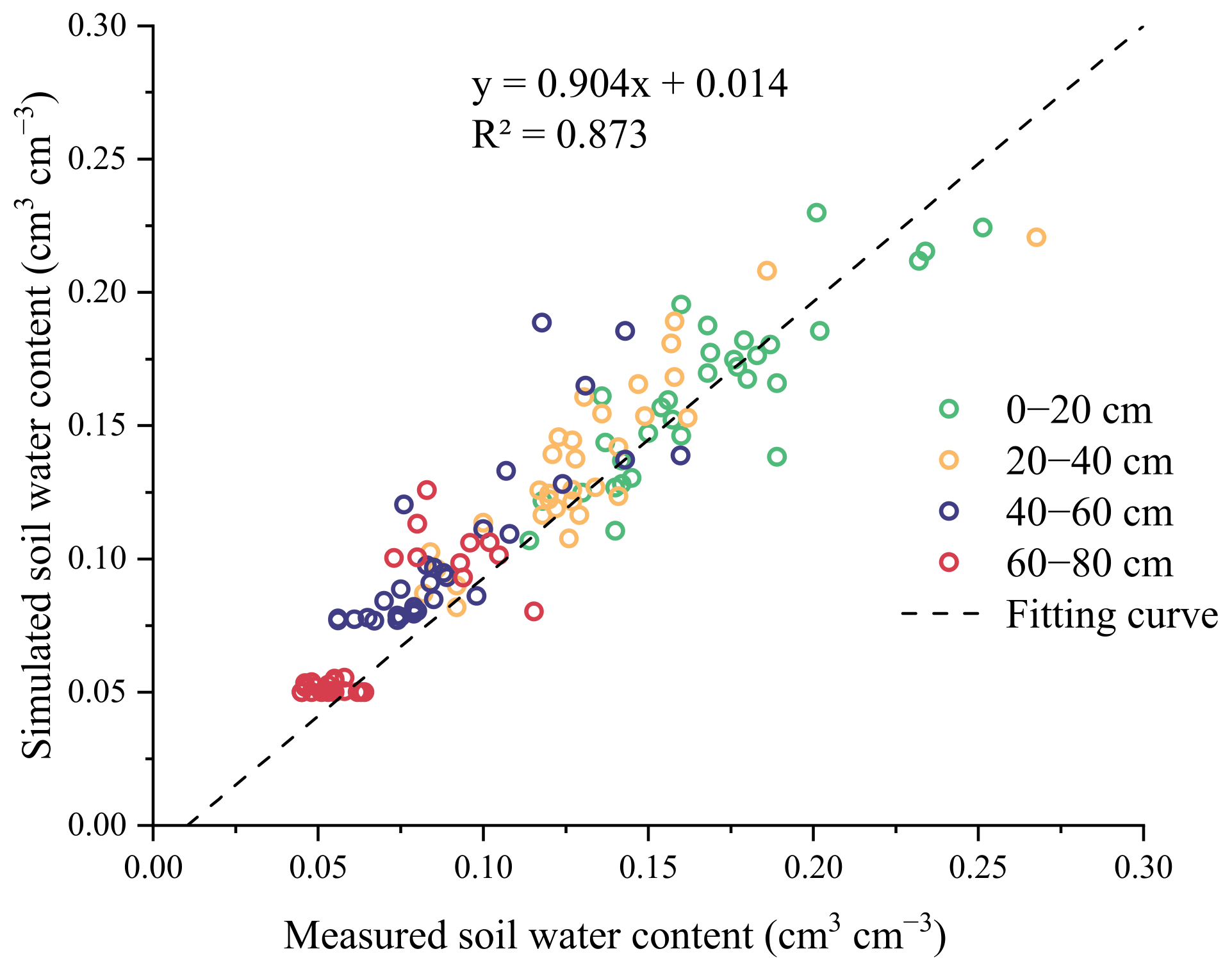
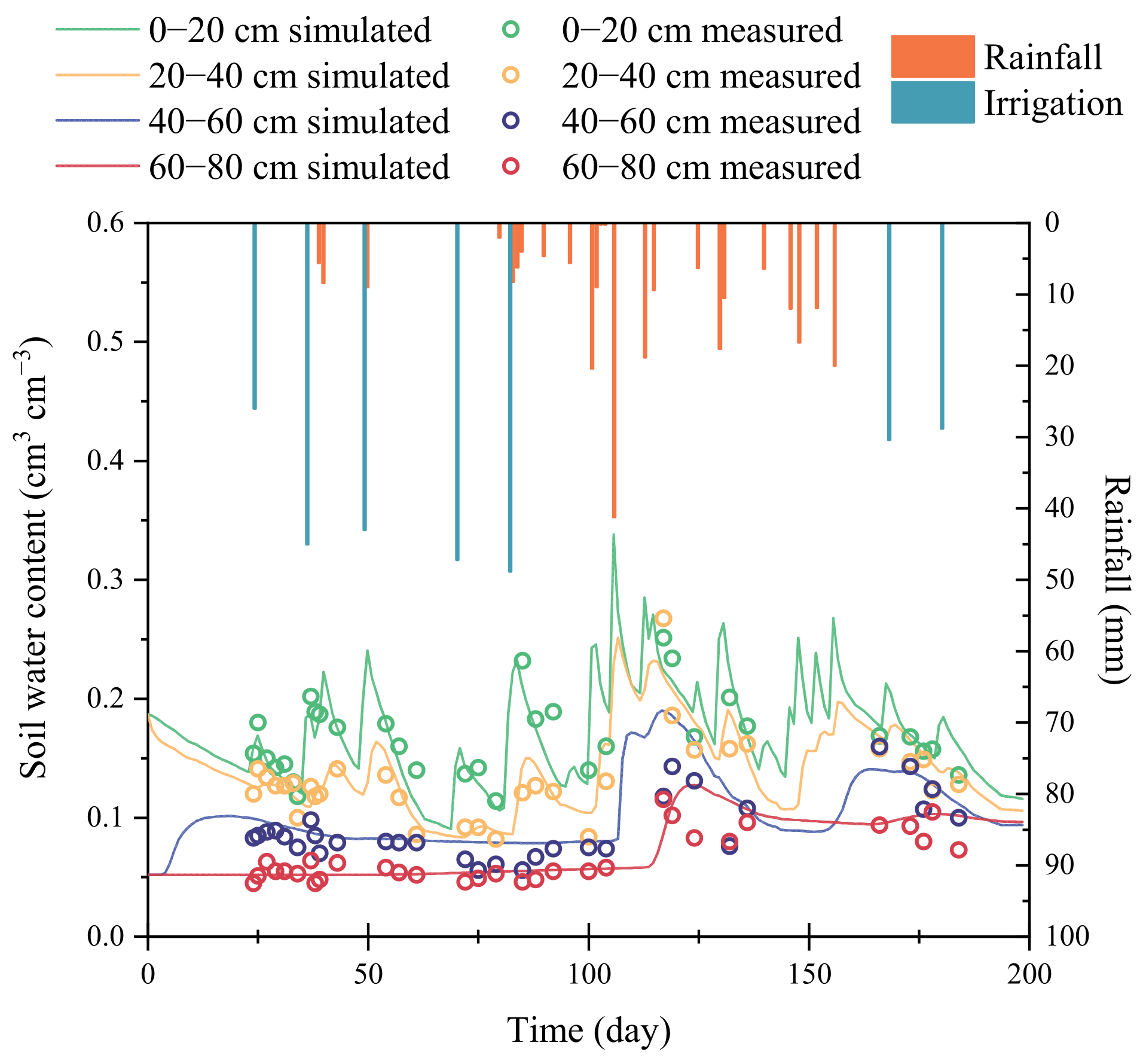
3.1. Model Validation

Numerical simulations for all of 2022 were performed based on the conditions of the field experiments. The model was preliminarily validated by comparing simulated and measured soil water content at corresponding times and locations. Figure 3 compares simulated and measured soil water contents throughout the alfalfa growing season, with an overall R² of 0.873, demonstrating a strong model fit. Figure 4 illustrates temporal variations in simulated and measured soil water content under the experiment conditions in 2022. Seven irrigation events were applied during the growing season, with a cumulative irrigation amount of 269 mm, while the total effective rainfall for the year was 254 mm. During the alfalfa growing period, the soil water content in the shallow layer fluctuated significantly with irrigation or rainfall, whereas the soil water content in deeper layers remained nearly constant before heavy rainfall. The primary simulation errors in shallow soil layer occurred after irrigation or rainfall, where the simulated soil water content was slightly lower than the measured values. However, the temporal patterns of soil water content throughout the growing season exhibited a high degree of consistency between simulated and measured values. Soil water content in deeper layers exhibited minimal fluctuations throughout the alfalfa growing season but was overestimated in the simulations during heavy rainfall events. This discrepancy may be attributed to surface runoff occurring during heavy rainfall under the actual field conditions, leading to reduced water infiltration into deeper soil layers compared to the simulated values.

A statistical analysis of the soil water content data at various depths for model validation is presented in

Table 2. Statistical analysis of soil water content for model verification.

Soil Depth/ cm	RMSE/ (cm3 cm−3)	NRMSE/ %	MAE/ (cm3 cm−3)	R2
0–20	0.018	10.6	0.014	0.731
20–40	0.017	12.8	0.013	0.783
40–60	0.021	23.2	0.014	0.697
60–80	0.014	21.8	0.009	0.675

Notes: The root-mean-square error (RMSE), normalized root-mean-square error (NRMSE), mean absolute error (MAE), and coefficient of determination (R²) were used to evaluate the model performance. RMSE and NRMSE quantify the absolute and relative differences between simulated and measured values, respectively, with lower values indicating higher simulation accuracy. NRMSE values below 30% are generally considered indicative of a reliable simulation.

. The RMSE values for simulated and measured soil water contents at each depth were all below 0.021 cm³/cm³, the NRMSE values did not exceed 23.3%, and the MAE values remained under 0.014 cm³/cm³, indicating that HYDRUS-2D exhibited low errors and a strong ability to capture dynamic variations in soil water content across different soil depths. Although the model errors were relatively larger in deeper soil layers, this had a minor impact on optimizing the system installation parameters and deficit irrigation schedules, given that alfalfa root water uptake and soil surface evaporation primarily occurred in the upper soil layers. Therefore, HYDRUS-2D was considered appropriate for relevant simulation and optimization analyses in this study.

3.2. Soil Water Movement

Using a commonly used drip-line installation distance of 75 cm and the F3 and W3 deficit irrigation schedule as examples, Figure 5 illustrates the temporal variations in irrigation and rainfall, alfalfa crop coefficients, and numerically simulated alfalfa root water uptake, soil surface evaporation, and soil water content at different depths throughout the entire growing season. As shown in Figure 5a,d, local rainfall was scarce during the first two alfalfa harvests, with soil water replenishment primarily relying on irrigation. During this period, soil water content in the planned wetting layer remained relatively stable, whereas soil water content in deeper soil layers remained consistently low. The rainy season occurred between the end of the second harvest and the beginning of the fourth harvest, during which period frequent rainfall reduced the need for irrigation. Meanwhile, soil water in shallow soil layers became saturated, and soil water content in deeper soil layers increased overall without significant deep percolation. The total deep percolation over the entire growing season was only 13.54 mm. According to the local climate conditions and irrigation scenarios, the variations in the alfalfa crop coefficient (K_c) and the basal crop coefficient (K_cb) throughout the entire growing season are shown in Figure 5b. Compared with the basal crop coefficient, the crop coefficient accounts for soil surface evaporation following irrigation and rainfall, resulting in an annual potential transpiration of 491.16 mm and a potential soil surface evaporation of 115.59 mm. The variations in the actual crop transpiration rate and soil surface evaporation rate are illustrated in Figure 5c. Overall, the transpiration rate of alfalfa initially increased and then stabilized between harvests, followed by a decline to a lower level after each harvest. Total transpiration was highest during the first and third harvests—the first harvest spanned a longer period, while the third harvest was unaffected by deficit irrigation due to abundant rainfall. During the second and fourth harvests, mild water stress was observed, making actual transpiration lower than potential transpiration. Over the entire growing season, the cumulative actual transpiration of alfalfa reached 529.80 mm, accounting for 87.32% of the potential evapotranspiration. Due to the highly permeable sandy texture of the shallow soil, soil surface evaporation primarily occurred within 3–5 days after irrigation or rainfall. Meanwhile, in the late growth stages of each harvest cycle, soil surface evaporation was suppressed and remained at a low level as the canopy cover increased. The total soil surface evaporation under this treatment was 113.68 mm, accounting for 21.46% of the actual evapotranspiration.

Figure 6 presents the simulation results under different deficit irrigation thresholds and irrigation depths for four drip-line installation distances. As the installation distance increased, alfalfa root water uptake gradually decreased, leading to a decrease in the ratio of actual transpiration to potential transpiration. Concurrently, a larger distance between drip lines reduced the proportion of soil surface wetted during each irrigation event, resulting in a continuous decrease in the ratio of soil evaporation to potential evapotranspiration. However, due to the complex interactions between root water uptake and soil evaporation, no clear pattern was observed between deep percolation and drip-line installation distance.

Overall, the drip-line installation distance had a minimal impact on irrigation performance, with each indicator exhibiting a consistent trend across the four drip-line installation distances. As the deficit irrigation threshold increased from F1 to F3, alfalfa root water uptake steadily rose, with an increase of 12.24% to 15.34% recorded across different scenarios. Additionally, actual evapotranspiration approached potential evapotranspiration under higher irrigation thresholds, indicating that reducing water stress enhanced alfalfa transpiration, which is beneficial for yield improvements. Meanwhile, as the deficit irrigation threshold increased, more frequent irrigation events led to increases in both soil evaporation and its proportion in actual evapotranspiration. At a 60 cm drip-line installation distance and W3 irrigation depth, increasing the irrigation threshold from F1 to F3 resulted in a 29.58% increase in soil evaporation. Furthermore, since root distribution was only defined within the 0–80 cm soil layer, water that infiltrated deeper was beyond the reach of the alfalfa roots. As a result, under the F2 or F3 irrigation thresholds, deep percolation was more likely to occur during heavy rainfall, especially in scenarios with higher irrigation depths, because the soil water content remained at a high level. On the other hand, increasing the irrigation depth reduced the proportion of soil evaporation in actual evapotranspiration and brought the actual evapotranspiration closer to the potential evapotranspiration. This occurred because soil evaporation per irrigation event did not significantly change with the irrigation depth, whereas larger irrigation depths markedly improved the root zone moisture conditions. Therefore, selecting a relatively higher irrigation depth is preferable, provided that excessive deep percolation does not occur.

Overall, under the current soil texture conditions and alfalfa root distribution, increasing the drip-line installation distance did not significantly affect irrigation performance or alfalfa root water uptake. However, smaller installation distances result in higher installation and operational maintenance costs. Therefore, adopting a wider drip-line installation distance for MDI systems appears to be more cost-effective. The focus of Pareto optimization lies in balancing the trade-offs between reducing deep percolation, saving irrigation water, and maximizing crop yield.

3.3. Multi-Objective Optimization Results

The NSGA-II multi-objective optimization algorithm was used to solve the problem, with a population size of 100, a mutation intensity of 0.1, a crossover probability of 0.8, a mutation probability of 0.1, and 80 iterations. The optimized results that satisfied the given constraints are presented in Figure 7. Figure 7A–D illustrate the relationships between the following parameters: (A) root water uptake and total irrigation amount; (B) root water uptake and soil surface evaporation; (C) deep percolation and soil surface evaporation; (D) soil surface evaporation and total irrigation amount within the solution set. Since the objective functions were normalized, the closer a dependent variable’s value in the objective space is to 1, the closer that indicator is to its optimal value. Due to the competitive nature of the objectives, the boundary formed by the non-dominated solutions in the objective space represents the Pareto front (green line in the figure), indicating that no solutions can be further optimized across all objectives. A linearly decreasing Pareto front is observed in Figure 7A, highlighting the strong conflict between reducing the total irrigation amount and increasing crop root water uptake. Similarly, enhancing root water uptake necessitated frequent irrigation to maintain soil moisture, thereby increasing soil surface evaporation. The Pareto fronts between different objective functions in Figure 7 provide multiple optimization directions for deficit irrigation schedule design. These Pareto fronts represent the set of optimal solutions under the given constraints, enabling decision-making based on specific factors such as expected yield and water resource availability.

To balance the optimization objectives, we propose a Pareto-optimal solution as the recommended deficit irrigation schedule for the local MDI system. The position of this Pareto solution in the objective space is indicated by the yellow dot in Figure 7. The corresponding decision variables are a drip-line installation distance of 105 cm, a deficit irrigation threshold of 50–55% FC, and an irrigation depth of 112% W. As analyzed earlier, a drip-line installation distance of 105 cm can significantly reduce system installation and maintenance costs without compromising the irrigation performance. The combination of a lower deficit irrigation threshold and a higher irrigation depth is similar to the F1 and W4 treatment. A lower deficit irrigation threshold helps to reduce soil surface evaporation and deep percolation, while a higher single irrigation depth ensures sufficient moisture for the alfalfa roots, thereby securing yield stability.

4. Discussion

This preliminary study investigated the optimal deficit irrigation schedule and drip-line installation distance for alfalfa under specific climatic and soil conditions by using HYDRUS-2D numerical simulations and multi-objective optimization with the NSGA-II algorithm. The MDI system is a relatively new water-saving irrigation technology, and extensive research has been conducted by scholars on its irrigation performance and water-saving potential for yield improvement [14,27,28]. Among these studies, Oker et al. [29] also used HYDRUS-2D to analyze water application uniformity and infiltration depth in MDI systems. However, their study did not account for crop root water uptake and soil surface evaporation, which limited its ability to provide recommendations for irrigation system design and scheduling under MDI conditions. Given the proven accuracy of HYDRUS-2D in simulating soil water movement across different irrigation scenarios, numerous researchers [19,20,30] have integrated this model with various optimization techniques to refine irrigation and fertilization strategies for different irrigation systems. This study fully considered the characteristics of high-flowrate localized irrigation in MDI systems, focusing on factors such as reducing soil surface evaporation and avoiding deep percolation to strategically leverage the advantages of MDI systems in system design and deficit irrigation scheduling. In this preliminary study, the multi-objective optimization algorithm was adopted to find a balance among multiple conflicting objectives through exploring the Pareto front. Hence, the optimization results represent a solution set of different trade-offs among the optimization objectives, rather than a specific optimal solution. The existence of the Pareto front revealed the conflicting relationships among the objectives, providing an intuitive basis for decision-making and adjustments. As shown in Figure 7A,B, increasing crop yield would increase the total irrigation amount and soil surface evaporation, a typical objective conflict phenomenon.

From a practical physical perspective, reducing the total irrigation amount can simultaneously decrease soil surface evaporation and deep percolation, indicating that these objectives may be synergistically optimized in reality. However, Pareto fronts still appear between objectives that do not directly conflict in Figure 7C,D. This may be due to the characteristics of multi-objective optimization: this study included four optimization objectives, and the sparse distribution of solutions in a high-dimensional objective space can lead to local non-dominance in projecting solutions onto one plane, thereby forming a Pareto front. On the other hand, there was a complex nonlinear relationship between the objective functions and the independent variables in this study. Even if two objectives can be synergistically optimized in reality, the “mathematical conflict” in the model may still result in the emergence of a Pareto front. Consequently, the Pareto fronts obtained in this study are reasonable. With respect to production application, different trade-off solutions can be selected based on actual needs, such as prioritizing crop yield or minimizing the total irrigation amount, thereby enhancing the practicality and decision support capability of this study.

As the experimental field was composed of backfilled soil, a gravel layer was presented below 80 cm. The gravel layer severely limited the downward extension of alfalfa roots, restricting the active rooting zone primarily to the upper soil layers. Therefore, this preliminary study focused on soil water dynamics and root water uptake behavior within the 0–80 cm soil layer in both field experiments and numerical simulations. A similar limitation was reported in the study by Wang et al. [31] at the same experimental site. However, under favorable conditions, alfalfa roots can extend to depths exceeding 6 m [32]. Even under typical field conditions, previous studies have documented that alfalfa roots may still extract water from depths of up to 2 m [33,34,35]. Given that the alfalfa in this study had been established for 3 years, it is possible that some roots might still access water below 80 cm, despite the presence of the gravel layer. In irrigation management, deep roots can significantly influence the irrigation strategies, particularly in assessing deep percolation. A greater rooting depth implies that larger irrigation depths and higher irrigation thresholds could potentially be considered in decision-making. Consequently, assuming a rooting zone strictly limited to 0–80 cm may result in an overestimation of deep percolation, as some water infiltrating below this depth could still be utilized by the crop. Future research should therefore investigate alfalfa root distribution in deeper soil layers to refine the irrigation strategies and enhance their applicability to typical alfalfa cultivation scenarios.

When optimizing deficit irrigation schedules, this study did so at an annual scale, simplifying the model while ensuring global optimization. However, annual-scale optimization ignores the variations in water demand across different alfalfa growth stages, thereby limiting the potential for water savings and yield improvements in the optimization results. Scholars such as Hanson et al. [36], Liu et al. [10], and Li et al. [37] applied differentiated deficit irrigation treatments across different seasons or growth stages of alfalfa and highlighted that this approach can avoid the negative impacts of water deficit during water-sensitive stages, such as the branching period, thereby achieving higher yields. Additionally, in northern China, the focus region of this study, different irrigation strategies are adopted before and after the rainy season, an approach that can balance the impact of heavy rainfall and further reduce deep percolation. Future research should further refine the irrigation strategies by integrating climate conditions and critical water demand periods within the crop growth cycle for dynamic optimization to ensure more precise water allocation and improve water use efficiency.

5. Conclusions

To fully harness the water-saving potential of MDI systems, this preliminary study conducted a one-year field experiment to validate HYDRUS-2D. The validated numerical model was then used to investigate the effects of four drip-line installation distances (60, 75, 90, and 105 cm), three deficit irrigation thresholds (45–50% FC, 55–60% FC, and 65–70% FC), and four irrigation depths (70% W, 85% W, 100% W, and 115% W) on root water uptake, soil surface evaporation, total irrigation amount, and deep percolation throughout the alfalfa growing season. Aiming to maximize alfalfa root water uptake while minimizing soil surface evaporation, deep percolation, and system costs, the NSGA-II multi-objective optimization algorithm was applied to perform Pareto optimization on drip-line installation distance, deficit irrigation thresholds, and irrigation depth in MDI systems. This study provides preliminary insight into irrigation optimization for alfalfa under MDI systems. Due to the presence of a gravel layer below 80 cm in the experimental field, root water uptake was only considered within the 0–80 cm soil layer in both field observations and numerical simulations. As a result, the present analysis is preliminary and based on site-specific constraints. Future research should investigate alfalfa root distribution in deeper soil layers to refine the irrigation strategies and improve their applicability to typical alfalfa cultivation scenarios.

The main results are summarized as follows:

(1)

The field experiment demonstrated that HYDRUS-2D can accurately simulate soil water movement using MDI systems, with the simulated values closely matching the measured values throughout the alfalfa growing season. The RMSE values of soil water content at all measured depths were all less than 0.021 cm³/cm³, with NRMSE values below 23.3%, and MAE values below 0.014 cm³/cm³.

(2)

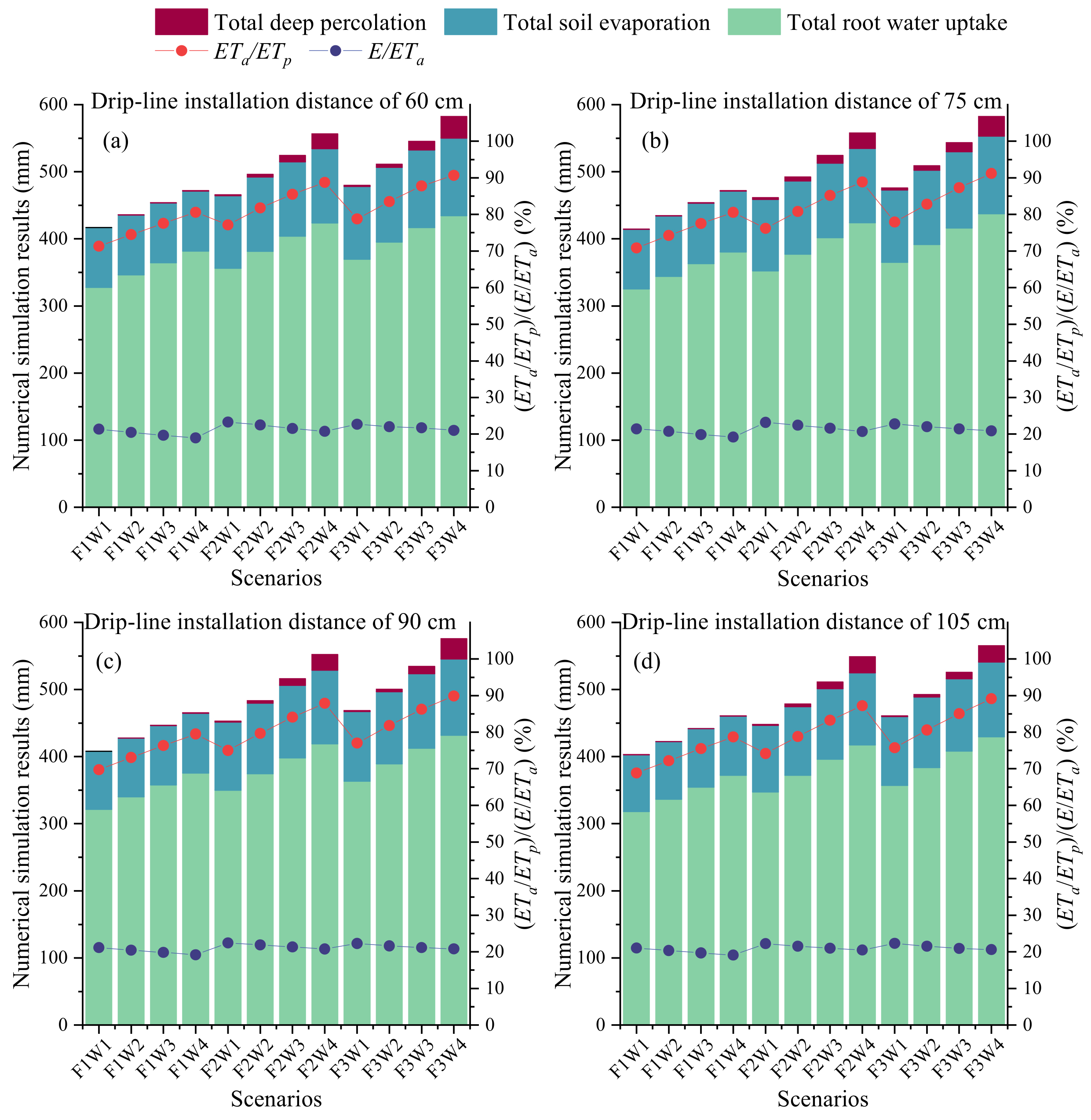
Under the current soil texture and crop conditions, the drip-line installation distance did not significantly affect the irrigation performance. However, increasing the deficit irrigation threshold from F1 to F3 enhanced alfalfa root water uptake by 12.24–15.34%, but this also increased the annual total irrigation amount, soil surface evaporation (by up to 29.58%), and the risk of deep percolation. Similar trends were observed with increasing irrigation depth. Thus, formulating irrigation schedules requires balancing these competing objectives.

(3)

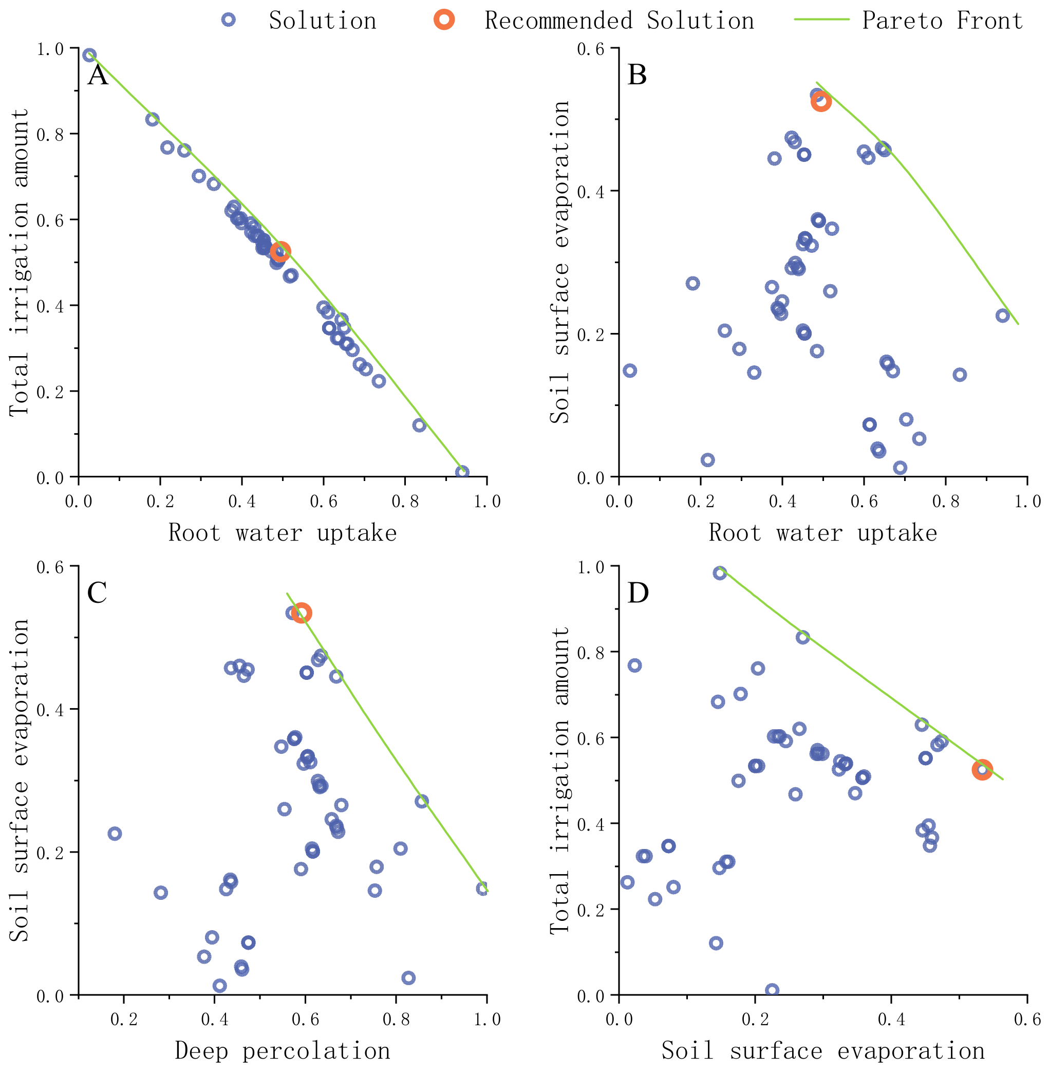
The NSGA-II multi-objective algorithm conducted Pareto optimization among multiple conflicting objectives, and the Pareto front in the results represents the trade-offs and compromises among the optimization objectives. For this case study, a drip-line installation distance of 105 cm, a deficit irrigation threshold of 50–55% FC, and an irrigation depth of 112% W are recommended to achieve a balance among the optimization objectives.

References

1. Salehi, M. Global water shortage and potable water safety; Today’s concern and tomorrow’s crisis. Environ. Int. 2022, 158, 106936. [Google Scholar] [CrossRef] [PubMed]
2. Shi, J.; Wu, X.; Zhang, M.; Wang, X.; Zuo, Q.; Wu, X.; Zhang, H.; Ben-Gal, A. Numerically scheduling plant water deficit index-based smart irrigation to optimize crop yield and water use efficiency. Agric. Water Manag. 2021, 248, 106774. [Google Scholar] [CrossRef]
3. Li, M.; Zhou, S.; Shen, S.; Wang, J.; Yang, Y.; Wu, Y.; Chen, F.; Lei, Y. Climate-smart irrigation strategy can mitigate agricultural water consumption while ensuring food security under a changing climate. Agric. Water Manag. 2024, 292, 108663. [Google Scholar] [CrossRef]
4. Fereres, E.; Soriano, M.A. Deficit irrigation for reducing agricultural water use. J. Exp. Bot. 2007, 58, 147–159. [Google Scholar] [CrossRef]
5. Li, Q.; Chen, Y.; Sun, S.; Zhu, M.; Xue, J.; Gao, Z.; Zhao, J.; Tang, Y. Research on crop irrigation schedules under deficit irrigation-a meta-analysis. Water Resour. Manag. 2022, 36, 4799–4817. [Google Scholar] [CrossRef]
6. Wu, W.; Liu, M.; Wu, X.; Wang, Z.; Yang, H. Effects of deficit irrigation on nitrogen uptake and soil mineral nitrogen in alfalfa grasslands of the inland arid area of China. Agric. Water Manag. 2022, 269, 107724. [Google Scholar] [CrossRef]
7. Bali, K.M.; Putnam, D.; Wang, D.; Begna, S.; Holder, B.; Mohamed, A.Z.; Paloutzian, L.; Dahlke, H.E.; Eltarabily, M.G. Midsummer deficit irrigation of alfalfa for water conservation in the San Joaquin Valley of California. J. Irrig. Drain. Eng. 2024, 150, 04024029. [Google Scholar] [CrossRef]
8. Wagle, P.; Gowda, P.H.; Northup, B.K. Dynamics of evapotranspiration over a non-irrigated alfalfa field in the Southern Great Plains of the United States. Agric. Water Manag. 2019, 223, 105727. [Google Scholar] [CrossRef]
9. Ismail, S.M.; Almarshadi, M.H. Maximizing productivity and water use efficiency of alfalfa under precise subsurface drip irrigation in arid regions. Irrig. Drain. 2013, 62, 57–66. [Google Scholar] [CrossRef]
10. Liu, M.; Wang, Z.; Mu, L.; Xu, R.; Yang, H. Effect of regulated deficit irrigation on alfalfa performance under two irrigation systems in the inland arid area of midwestern China. Agric. Water Manag. 2021, 248, 106764. [Google Scholar] [CrossRef]
11. Zhang, H.; Yan, H.; Hui, X.; Zhao, H.; Wang, W.; Guo, H. Experiments and numerical simulations of soil water movement under mobile drip irrigation system. Trans. Chin. Soc. Agric. Eng. 2023, 39, 158–168. (In Chinese) [Google Scholar]
12. Koudahe, K.; Aguilar, J.; Djaman, K.; Sheshukov, A.Y. Evapotranspiration, fiber yield and quality, and water productivity of cotton (Gossypium hirsutum L.) under different irrigation technologies in a semiarid climate. Irrig. Sci. 2024, 42, 575–594. [Google Scholar] [CrossRef]
13. Kisekka, I.; Oker, T.; Nguyen, G.; Aguilar, J.; Rogers, D. Revisiting precision mobile drip irrigation under limited water. Irrig. Sci. 2017, 35, 483–500. [Google Scholar] [CrossRef]
14. Oker, T.E.; Kisekka, I.; Sheshukov, A.Y.; Aguilar, J.; Rogers, D. Evaluation of dynamic uniformity and application efficiency of mobile drip irrigation. Irrig. Sci. 2020, 38, 17–35. [Google Scholar] [CrossRef]
15. Soto, A.L.; Shrestha, R.; Xue, Q.; Colaizzi, P.; O’Shaughnessy, S.; Workneh, F.; Adhikari, R.; Rush, C. Evaluation of three irrigation application systems for watermelon production in the Texas High Plains. Agron. J. 2024, 116, 2535–2550. [Google Scholar] [CrossRef]
16. O’Shaughnessy, S.A.; Colaizzi, P.D. Performance of precision mobile drip irrigation in the Texas High Plains Region. Agronomy 2017, 7, 68. [Google Scholar] [CrossRef]
17. Holt, J.; Yost, M.; Creech, E.; Winward, D.; Barker, B. On-farm evaluations of overhead irrigation sprinkler packages at full and reduced rates. Soil Sci. Soc. Am. J. 2024, 88, 152–165. [Google Scholar] [CrossRef]
18. Dabach, S.; Shani, U.; Lazarovitch, N. Optimal tensiometer placement for high-frequency subsurface drip irrigation management in heterogeneous soils. Agric. Water Manag. 2015, 152, 91–98. [Google Scholar] [CrossRef]
19. Kandelous, M.M.; Kamai, T.; Vrugt, J.A.; Simunek, J.; Hanson, B.; Hopmans, J.W. Evaluation of subsurface drip irrigation design and management parameters for alfalfa. Agric. Water Manag. 2012, 109, 81–93. [Google Scholar] [CrossRef]
20. Azad, N.; Behmanesh, J.; Rezaverdinejad, V.; Abbasi, F.; Navabian, M. Developing an optimization model in drip fertigation management to consider environmental issues and supply plant requirements. Agric. Water Manag. 2018, 208, 344–356. [Google Scholar] [CrossRef]
21. Feddes, R.A.; Kowalik, P.I.; Zaradny, H. Simulation of Field Water Use and Crop Yield; John Wiley & Sons: New York, NY, USA, 1978. [Google Scholar]
22. Allen, R.G.; Pereira, L.S.; Raes, D.; Smith, M. Crop evapotranspiration: Guidelines for computing crop water requirements. In Irrigation and Drainage Paper No. 56; United Nations FAO: Rome, Italy, 1998; pp. 24–28. [Google Scholar]
23. Taylor, S.A.; Ashcroft, G.M. Physical Edaphology; Freeman and Co.: San Francisco, CA, USA, 1972; pp. 434–435. [Google Scholar]
24. Vrugt, J.A.; Hopmans, J.W.; Šimùnek, J. Calibration of a two-dimensional root water uptake model. Soil Sci. Soc. Am. J. 2001, 65, 1027–1037. [Google Scholar]
25. Jiang, R.; He, W.; He, L.; Yang, J.Y.; Qian, B.; Zhou, W.; He, P. Modelling adaptation strategies to reduce adverse impacts of climate change on maize cropping system in Northeast China. Sci. Rep. 2021, 11, 810. [Google Scholar]
26. Zhao, W.; Ma, F.; Cao, W.; Ma, F.; Han, L. Effects of water and fertilizer coupling on the yield and quality of tomatoes. Trans. Chin. Soc. Agric. Eng. 2022, 38, 95–101. (In Chinese) [Google Scholar]
27. Reynolds, S.; Guerrero, B.; Golden, B.; Amosson, S.; Marek, T.; Bell, J.M. Economic feasibility of conversion to mobile drip irrigation in the Central Ogallala region. Irrig. Sci. 2020, 38, 569–575. [Google Scholar] [CrossRef]
28. Oker, T.E.; Kisekka, I.; Sheshukov, A.Y.; Aguilar, J.; Rogers, D.H. Evaluation of maize production under mobile drip irrigation. Agric. Water Manag. 2018, 210, 11–21. [Google Scholar] [CrossRef]
29. Oker, T.E.; Sheshukov, A.Y.; Aguilar, J.; Rogers, D.H.; Kisekka, I. Evaluating soil water redistribution under mobile drip irrigation, low-elevation spray application, and low-energy precision application using HYDRUS. J. Irrig. Drain. Eng. 2021, 147, 04021016. [Google Scholar] [CrossRef]
30. Bristow, K.L.; Simunek, J.; Helalia, S.A.; Siyal, A.A. Numerical simulations of the effects furrow surface conditions and fertilizer locations have on plant nitrogen and water use in furrow irrigated systems. Agric. Water Manag. 2020, 232, 106044. [Google Scholar] [CrossRef]
31. Wang, Y.; Li, M.; Guo, J.; Yan, H. Alfalfa (Medicago sativa L.) Nitrogen utilization, yield and quality respond to nitrogen application level with center pivot fertigation system. Agronomy 2024, 14, 48. [Google Scholar] [CrossRef]
32. Undersander, D.; Cosgrove, D.; Cullen, E.; Grau, C.; Rice, M.E.; Renz, M.; Sheaffer, C.; Shewmaker, G.; Sulc, M. Alfalfa Management Guide; American Society of Agronomy; Crop Science Society of America; Soil Science Society of America: Madison, WI, USA, 2011. [Google Scholar]
33. Clement, C.; Sleiderink, J.; Svane, S.F.; Smith, A.G.; Diamantopoulos, E.; Desbroll, D.B.; Thorup-Kristensen, K. Comparing the deep root growth and water uptake of intermediate wheatgrass (Kernza) to alfalfa. Plant Soil 2022, 472, 369–390. [Google Scholar] [CrossRef]
34. McCallum, M.H.; Connor, D.J.; O’Leary, G.J. Water Use by Lucerne and Effect on Crops in the Victorian Wimmera. Aust. J. Agric. Res. 2001, 52, 193–201. [Google Scholar] [CrossRef]
35. Ward, P.R.; Dunin, F.X.; Micin, S.F. Water use and root growth by annual and perennial pastures and subsequent crops in a phase rotation. Agric. Water Manag. 2002, 53, 83–97. [Google Scholar] [CrossRef]
36. Hanson, B.; Bali, K.; Orloff, S.; Carlson, H.; Sanden, B.; Putnam, D. Midsummer deficit irrigation of alfalfa as a strategy for providing water for water—Short areas. Sustain. Irrig. Manag. Technol. Policies II 2008, 112, 115. [Google Scholar] [CrossRef]
37. Li, M.; Zhang, Y.; Ma, C.; Sun, H.; Ren, W.; Wang, X. Maximizing the water productivity and economic returns of alfalfa by deficit irrigation in China: A meta-analysis. Agric. Water Manag. 2023, 287, 108454. [Google Scholar] [CrossRef]
Figure 1. Average monthly meteorological data recorded during the experimental period at a meteorological station approximately 150 m from the experimental site.
Water 17 00966 g001
Figure 2. A schematic diagram of the HYDRUS-2D computational domain, showing the sandy loam soil profile (0–80 cm, with increasing gravel content from 40 to 80 cm), the underlying gravel layer (below 80 cm), and the boundary conditions (AF and DE: zero-flux boundaries; AB and CD: infiltration boundaries during irrigation events, atmospheric boundaries during non-irrigation periods; BC: atmospheric boundary; EF: free drainage boundary).
Water 17 00966 g002
Figure 3. Comparison of measured and simulated soil water contents at various depths.
Water 17 00966 g003
Figure 4. Temporal variations in simulated and measured soil moisture content, with rainfall and irrigation events as a reference.
Water 17 00966 g004
Figure 5. Temporal variations in key indicators throughout the alfalfa growing season: (a) rainfall and irrigation; (b) alfalfa crop coefficient (Kc) and basal crop coefficient (Kcb); (c) root water uptake and evaporation; (d) soil water content at different depths.
Water 17 00966 g005
Figure 6. Numerical simulation results for different irrigation thresholds and irrigation depths across four drip-line installation distances: (a) 60 cm; (b) 75 cm, (c) 90 cm, and (d) 105 cm. ETa, ETp, and E represent the actual evapotranspiration, potential evapotranspiration, and evaporation, respectively. F1, F2, and F3 represent deficit irrigation thresholds of 45–50% FC, 55–60% FC, and 65–70% FC, respectively. W1, W2, W3, and W4 represent irrigation depths of 70% W, 85% W, 100% W, and 115% W, respectively. The irrigation amount (W) was determined based on the difference between the average soil water content in the planned wetting layer at irrigation initiation and 90% FC.
Water 17 00966 g006
Figure 7. Multi-objective optimization results illustrating trade-offs between (A) total irrigation amount and root water uptake, (B) soil surface evaporation and root water uptake, (C) soil surface evaporation and deep percolation, and (D) total irrigation amount and soil surface evaporation.
Water 17 00966 g007