Modeling Nitrogen Migration Characteristics in Cool-Season Turf Grass Soils via HYDRUS-2D

Abstract

In order to study the leaching of exogenous nitrogen during green space management and maintenance, the parameters of the model were calibrated through field monitoring and grow box simulation experiments, and the Model for Studying Nitrogen Transport in Green Space Ecosystems was established by using HYDRUS-2D software. Results showed that the model is highly reliable for simulating nitrogen transport in microtopography, with R² values greater than 0.9 and RMSE values below 5. Slope gradient was positively correlated with horizontal nitrogen differences (ammonium and nitrate nitrogen) and negatively correlated with vertical differences (p < 0.05), while nitrogen application was positively correlated with both horizontal and vertical differences in nitrate nitrogen and negatively correlated with ammonium nitrogen (p < 0.05). The vertical differences of soil ammonium nitrogen exhibited a significant negative correlation with slope (−0.837 to −0.851), while the horizontal differences of nitrate nitrogen showed a significant positive correlation, with correlation coefficients of 0.965 and 0.967 for surface and subsurface soils, respectively. The increasing nitrogen application rate exacerbated these discrepancies, with the highest nitrogen treatment (0.312 g) exhibiting the most pronounced differential effects. Notably, the horizontal variation in nitrate nitrogen reached 6.9-fold that of ammonium nitrogen, while the vertical discrepancy demonstrated a 7.0-fold magnitude relative to ammonium nitrogen levels.

1. Introduction

In 2022, China’s urban green space area reached 358.6 × 10⁸ m², in which the park green space area was 86.85 × 10⁸ m², accounting for approximately 24% [1]. The increase in the construction of urban green spaces and the sharp increase in investment into green space maintenance and management has improved the human well-being index but has also brought about new environmental challenges in urban areas. The long-term maintenance of lawn microterrain often involves the input of large amounts of fertilizer, and the intensive management and maintenance of lawns are increasing nonpoint source pollution (NPSP) from these green spaces.

Nitrogen is an important nutrient indispensable to the growth and development of turfgrass, and Mills and Jones reported that the nitrogen content of turfgrass stem and leaf tissues accounts for approximately 2–6% of the total nitrogen content of the plants; thus, the demand for nitrogen fertilizer is greatest during the growth of turf [2,3]. The addition of nitrogen can result in a higher growth density, extend the ornamental period of the lawn, and improve the ability of the lawn to resist pests and diseases and cope with environmental stressors [4]. However, excessive nitrogen availability has been shown to exacerbate plant disease incidence in numerous landscape studies. These findings underscore the critical need for precision-based nitrogen management strategies to optimize plant health while minimizing pathogenic risks [5]. Nitrogen, an exogenous nutrient prone to depletion due to anthropogenic activities, exhibits nitrogen use efficiency (NUE) ranging from 21 to 69% globally. For instance, developed countries like the USA and Europe achieve NUEs of 66–69% through optimized nutrient management, whereas China and India report significantly lower rates (21–35%) due to intensive farming practices and imbalanced nitrogen input [6]. Recent studies [7] have demonstrated that precision fertilization and organic amendments can enhance NUE by 15–30% in tree species like poplar, highlighting synergistic strategies for urban greening systems”. This unutilized nitrogen can migrate into the surrounding environment [8]; in particular, the loss of soil nutrient elements has a pronounced negative impact on the quality of groundwater [9]. After nitrogen fertilizer is applied to soil, it enters water bodies through subsurface infiltration from surface runoff and precipitation or irrigation, and the resulting NPSP has become one of the main sources of surface water and groundwater pollution worldwide [10]. Therefore, conducting research on nitrogen migration in turfgrass soils enables the characterization of nitrogen distribution and utilization patterns within urban green spaces, thereby achieving the goals of precision nitrogen application and scientific management.

Numerical modeling is one of the main methods used to study nitrogen transport processes, and many nitrogen transport models have been established and developed. The nitrogen conversion module in the HYDRUS-2D model can accurately simulate the interconversion of urea, ${\mathrm{N}\mathrm{H}}_4^{+}-\mathrm{N}$, and ${\mathrm{N}\mathrm{O}}_3^{-}-\mathrm{N}$ [11,12]. Most scholars have adopted the HYDRUS-2D model to simulate and verify the distributions of water and solute in irrigated land [13,14]. A few scholars have used the HYDRUS-2D model to simulate the nitrogen distribution in farmlands. The HYDRUS-2D model was used to simulate nitrogen uptake and transport under ridges and furrows during the maize growth period. The predicted distributions of soil water, nitrate, and ammonium nitrogen were in good agreement with the measured values [15]. The HYDRUS-2D model was also used to simulate the distributions of moisture, ${\mathrm{N}\mathrm{H}}_4^{+}-\mathrm{N}$, and ${\mathrm{N}\mathrm{O}}_3^{-}-\mathrm{N}$ in the wheat root zone over time under different tillage conditions [16]. Due to the coupled hydrodynamic and nitrogen transport/transform mechanisms in HYDRUS-2D, particularly its modular design that flexibly adapts to diverse land use types and microtopographic conditions, this model provides exceptional suitability for simulating nitrogen loss patterns in garden microtopography at high spatial resolution.

Few studies have looked at predicting exogenous nitrogen loss from microterrain turf. This is really important for fine-scale garden management and upkeep. Zhengzhou Green Expo Park is the study area. We added exogenous nitrogen to outdoor grow boxes, used HYDRUS-2D to build a nitrogen transport model for the study, and can now predict nitrogen loss for garden management. This is highly important for the fine-scale management and maintenance of gardens.

2. Materials and Methods

2.1. Grow Box Simulation Test

2.1.1. Soil Sample Collection and Analysis

The test area was located in the interior of Greening Expo Park in Zhengzhou New District, and three parallel sampling areas were set up for field inspection of the soil conditions at the test site of the park. After the establishment of the sampling area, surface vegetation was removed, a 0.3 m pit was dug to expose the soil profile, and samples were collected from 0 to 10 cm and 10–20 cm layers of the original soil via a ring knife. After natural air-drying, plant roots and gravel of various particle sizes were removed, and after soil sieving, the soil capacity, soil texture, soil saturated water content, physical and chemical properties of the soil, and other indices were examined. The detailed test results are shown in

Table 1. Basic Physical and Chemical Properties of Soil.

Depth	Soil Bulk Density	${\mathbf{N}\mathbf{O}}_3^{-}-\mathbf{N}$	${\mathbf{N}\mathbf{H}}_4^{+}-\mathbf{N}$	Clay	Silt	Sand
[cm]	[g·cm−3]	[mg·cm−3]	[mg·cm−3]	[%]	[%]	[%]
0–10	1.547	10.163	6.064	25.76	21.16	53.08
10–20	1.622	13.439	3.485	29.63	21.34	49.03

.

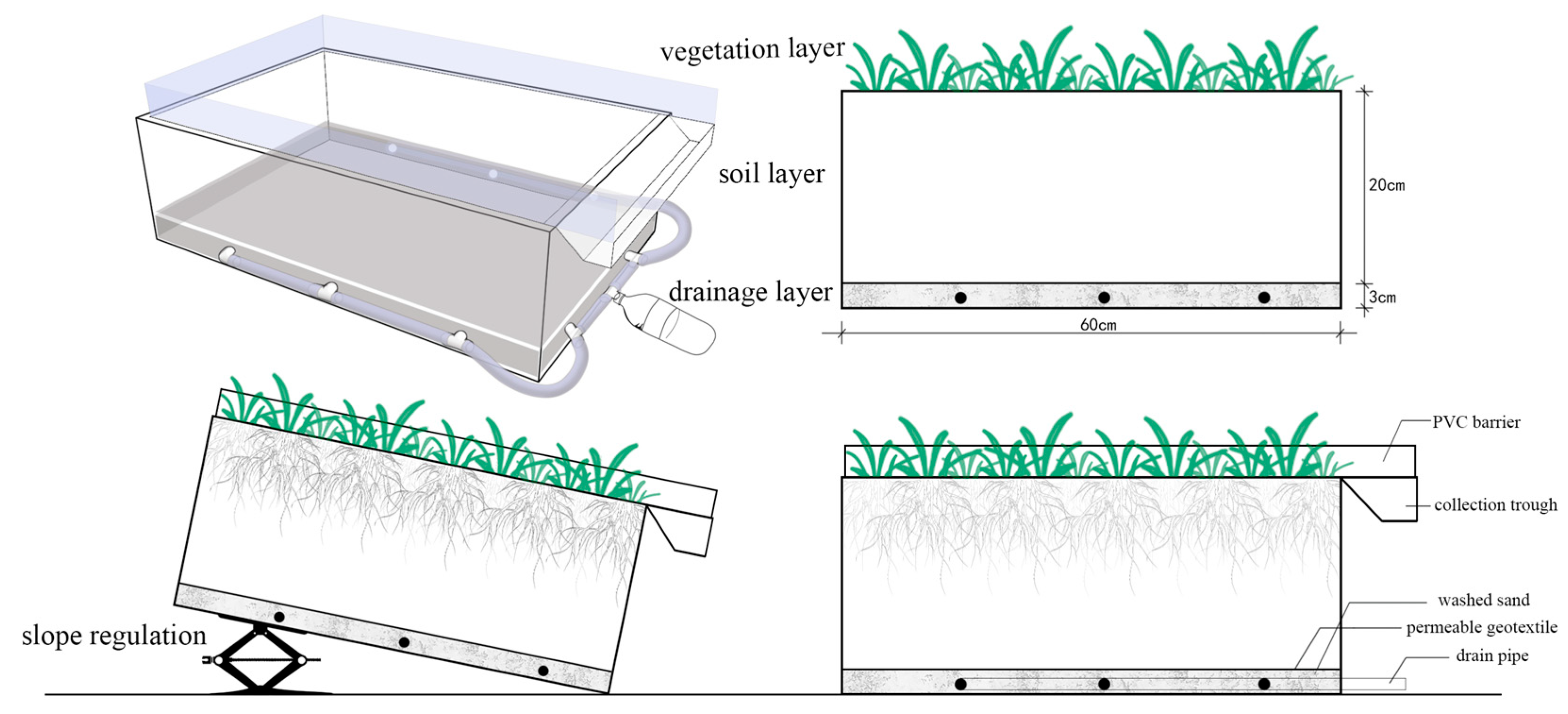
2.1.2. Design of the Test Device

The structure of the test device is shown in Figure 1. The size of the test grow box was 60 cm long, 40 cm wide, and 23 cm high. Eight drainage holes were uniformly located on the bottom of the grow box, gauze was wrapped around the drainage outlet to prevent blockage, the drainage holes were connected to a PVC hose, and the drainpipe terminals were connected to the collection device, which was used for the collection of the leached solution. The bottom of the grow box was evenly covered with washed sand with a particle size of 3–5 mm at a thickness of 3 cm to ensure that the water infiltrating during irrigation could be discharged easily. A permeable geotextile was laid over the washed sand to separate the test soil layer from the washed sand, the original soil from the site at a 0–20 cm depth was fully mixed and placed in the grow box, and each layer of soil was compacted to achieve soil density close to that in the natural state. The next layer of soil was laid up to a distance of 3–4 cm from the upper boundary, which is in accordance with the methods for grass seed sowing, mulching, and maintenance for lawn establishment. The grow box was set up according to the slope gradient results from the field research at Green Expo Park, and the grow box was redesigned with additional baffles and water catchment tanks for the collection of runoff from the slopes.

2.1.3. Test Methods

In this study, the change in and loss of nitrogen from lawn soil were investigated via a grow box simulation test with 40 days as the benchmark for the maintenance cycle. For the slope gradient characteristics of the study area, the slope gradient was divided into three levels of 2.9°, 8.1°, and 15.3°, and a no-slope control group i0 was set up. Five nitrogen treatments were set up for each slope group according to the nitrogen inputs in the management and maintenance standards (

Table 2. Standards for landscape and green space management and maintenance in Henan Province.

Lawn Maintenance Quota	Primary Maintenance		Secondary Maintenance		Tertiary Maintenance
	Warm-Season Turf Grass	Cool-Season Turf Grass	Warm-Season Turf Grass	Cool-Season Turf Grass	Warm-Season Turf Grass	Cool-Season Turf Grass
urea [kg]	6.600	13.20	4.400	8.800	4.400	8.800
Water [m3]	66.20	93.76	56.18	81.23	51.16	71.22

), and the amount of nitrogen applied to each group in a maintenance cycle was 0.128 g, 0.174 g, 0.22 g, 0.266 g, and 0.312 g, which were recorded as N1, N2, N3, N4, and N5, respectively. To ensure the uniformity of fertilizer application, manual spraying was carried out for fertigation. This was accomplished by dissolving the urea required for each treatment in 2000 mL of water and then uniformly spraying the solution onto each grow box. Spillage of the fertilizer solution was minimized during the spraying process, and the runoff as well as the leached solution was collected to determine the effect of the slope gradient on fertilizer loss. During the maintenance cycle, transparent plastic sheeting was used to intercept rainfall without blocking sunlight to avoid interference from natural rainfall during the experiment. Irrigation and maintenance of the 20 grow boxes followed the average standards for the study area in March–June, that is, irrigate every five days, with a volume of 2000 mL for a single grow box and an irrigation water flow rate of 15 mL/s. During irrigation, runoff in the water collection trough and soil leachate were collected separately, and the concentrations of ammonium nitrogen and nitrate nitrogen in the water samples were determined. Repeated soil collection was carried out with an earth auger at the top (T) and bottom (B) of the grow box slopes at depths of 5 and 15 cm, respectively, at the end of each irrigation session (Figure 2), and the samples were used to test the contents of ammonium nitrogen and nitrate nitrogen in the soil. During the maintenance cycle, there were eight irrigation and soil sampling sessions. After sampling, the soil was backfilled and reseeded with grass. Every 13 days, the turfgrass was manually trimmed. Grass clippings from the fixed area untreated spots were gathered, measured, and weighed to assess the growth rate of the turfgrass. This process was repeated three times within the cycle.

2.2. HYDRUS-2D Model Construction

2.2.1. Basic Equations of the Model

Soil Moisture Movement Equation

Simulations were conducted using HYDRUS 2D/3D Pro (version 2.04). In this study, the commonly used van Genuchten-Mualem (VG-M) soil hydraulic model was chosen as the parametric equation for soil moisture movement [4,17], which was used for numerical simulation of soil moisture and was modeled as shown in the following equation:

$$\theta \left(h\right)=\left\{\begin{array}{c}{\theta }_r+{\displaystyle \frac{{\theta }_s-{\theta }_r}{{\left[1+{\left|\alpha h\right|}^n\right]}^m}} , h<0\\ {\theta }_s , h>0\end{array}\right.$$

(1)

$$K\left(h\right)=K_s{S}_e^l{[1-(1-S_e^{1/m}\left)\right]}^2$$

(2)

Among them:

$$m=1-{\displaystyle \frac{1}{n}} , n>1$$

(3)

$$S_e={\displaystyle \frac{\theta -{\theta }_r}{{\theta }_s-{\theta }_r}}$$

(4)

where ${\theta }_S$ is the saturated water content (${{\mathrm{c}\mathrm{m}}^3·\mathrm{c}\mathrm{m}}^{-3}$); ${\theta }_r$ is the residual water content (${{\mathrm{c}\mathrm{m}}^3·\mathrm{c}\mathrm{m}}^{-3}$); $h$ is the pressure head (cm); $\alpha$ is the reciprocal of inlet suction (${\mathrm{c}\mathrm{m}}^{-1}$); $K_s$ is the saturated hydraulic conductivity (${\mathrm{c}\mathrm{m}·\mathrm{d}}^{-1}$); $S_e$ is the effective soil water content; $\mathit{l}$ is the pore connectivity parameter, which generally takes a value of 0.5; $m$ is the characteristic water curve parameter; and $n$ is the pore size distribution parameter.

Solute Transport Equation

After exogenous nitrogen is added to soil, ammonia-oxidizing microorganisms first oxidize ${\mathrm{N}\mathrm{H}}_4^{+}$ to ${\mathrm{N}\mathrm{O}}_2^{-}$, and then nitrite-oxidizing microorganisms oxidize ${\mathrm{N}\mathrm{O}}_2^{-}$ to ${\mathrm{N}\mathrm{O}}_3^{-}$ [17].

Fertilizer in soil moves and changes mainly through a first-order decay reaction. So, the model simulation uses the convection-dispersion equation (CDE) to describe this process [18]. Here is how it works in the model:

$${\displaystyle \frac{𝜕\theta C}{𝜕t}}+\mathsf{\rho }{\displaystyle \frac{𝜕s}{𝜕t}}={\displaystyle \frac{𝜕(\theta D\frac{𝜕C}{𝜕x})}{𝜕x}}-{\displaystyle \frac{𝜕qC}{𝜕x}}-S$$

(5)

where $C$ is the liquid phase concentration of the solute (${\mathrm{g}·\mathrm{c}\mathrm{m}}^{-3}$); $\mathit{s}$ is the solid phase concentration of the solute ($\mathrm{g}·{\mathrm{g}}^{-1}$); $D$ is the soil dispersion coefficient; $q$ is the water flux (${\mathrm{c}\mathrm{m}·\mathrm{s}}^{-1}$); and $S$ is the source-sink term ($\mathrm{g}·{\mathrm{c}\mathrm{m}}^{-3}·{\mathrm{s}}^{-1}$) $\theta$ is the Soil moisture content.

Considering the nitrification and denitrification processes of nitrogen and the uptake of nitrogen by the plant, the source-sink term for nitrate nitrogen in the above convection—dispersion equation $S_1$ was as follows:

$${S_1=k}_1\theta C_2-S_w{C}_{u1}{-k}_2\theta C_1$$

(6)

where $C_1$ is the ${\mathrm{N}\mathrm{O}}_3^{-}-\mathrm{N}$ concentration in the soil solution (${\mathrm{m}\mathrm{g}·\mathrm{L}}^{-1}$); $C_2$ is the ${\mathrm{N}\mathrm{H}}_4^{+}-\mathrm{N}$ concentration in the soil solution (${\mathrm{m}\mathrm{g}·\mathrm{L}}^{-1}$); $k_1$ is the rate of nitrification of ammonium nitrogen (${\mathrm{d}}^{-1}$); $k_2$ is the rate of denitrification of nitrate nitrogen (${\mathrm{d}}^{-1}$); $S_w$ is the root water uptake ($\mathrm{c}{{\mathrm{m}}^3·\mathrm{c}{\mathrm{m}}^3·\mathrm{d}}^{-1}$); and ${\mathit{C}}_{\mathit{u}1}$ is the root water uptake of nitrate nitrogen (${\mathrm{m}\mathrm{g}·\mathrm{L}}^{-1}$).

On the basis of the above equations combined with the actual conditions of the test, for ${\mathrm{N}\mathrm{O}}_3^{-}-\mathrm{N}$, the convection—dispersion equation was as follows:

$${\displaystyle \frac{𝜕\theta C_1}{𝜕t}}={\displaystyle \frac{𝜕}{𝜕z}}\left[\theta D{\displaystyle \frac{𝜕C_1}{𝜕z}}\right]-{\displaystyle \frac{𝜕q{C}_1}{𝜕z}}+\left(k_1\theta C_2-S_w{C}_{u1}{-k}_2\theta C_1\right)$$

(7)

where $C_1$ represents the ${\mathrm{N}\mathrm{O}}_3^{-}-\mathrm{N}$ concentration in the soil solution (${\mathrm{m}\mathrm{g}·\mathrm{L}}^{-1}$); $C_2$ represents the ${NH}_4^{+}-N$ concentration in the soil solution (${\mathrm{m}\mathrm{g}·\mathrm{L}}^{-1}$); $D$ represents the soil dispersion coefficient; $q$ represents the water flux (${\mathrm{c}\mathrm{m}·\mathrm{s}}^{-1}$); and $z$ represents the spatial coordinate.

Considering that soil organic nitrogen releases ammonium ions upon mineralization [19,20] and that ammonium nitrogen is easily adsorbed by soil colloids and absorbed by vegetation roots, the source-sink term for ammonium nitrogen in the above convection—dispersion equation $S_2$ was as follows:

$${S_2=k}_0\theta C_0-S_w{C}_{u2}{-k}_1\theta C_2$$

(8)

where $C_0$ represents the soil organic nitrogen content (${\mathrm{m}\mathrm{g}·\mathrm{L}}^{-1}$); $k_0$ represents the mineralization rate of organic nitrogen (${\mathrm{d}}^{-1}$); ${\mathit{k}}_1$ represents the nitrification rate of ammonium nitrogen (${\mathrm{d}}^{-1}$); ${\mathit{S}}_{\mathit{w}}$ represents the rate of root water uptake ($\mathrm{c}{{\mathrm{m}}^3·\mathrm{c}{\mathrm{m}}^3·\mathrm{d}}^{-1}$); and $C_{u2}$ represents the amount of ammonium nitrogen removed via root uptake (${\mathrm{m}\mathrm{g}·\mathrm{L}}^{-1}$).

For ${\mathrm{N}\mathrm{H}}_4^{+}-\mathrm{N}$, the convection—dispersion equation was

$${\displaystyle \frac{𝜕\theta C_2}{𝜕t}}+{\displaystyle \frac{𝜕{\rho sC}_2}{𝜕t}}={\displaystyle \frac{𝜕}{𝜕z}}\left[\theta D{\displaystyle \frac{𝜕C_2}{𝜕z}}\right]-{\displaystyle \frac{𝜕q{C}_2}{𝜕z}}+\left(k_3\theta C_0-S_w{C}_{u2}{-k}_1\theta C_2\right)$$

(9)

where $C_2$ represents the ${\mathrm{N}\mathrm{H}}_4^{+}-\mathrm{N}$ concentration in the soil solution (${\mathrm{m}\mathrm{g}·\mathrm{L}}^{-1}$); $\rho$ represents the soil bulk weight (${\mathrm{g}·\mathrm{c}\mathrm{m}}^{-3}$); $D$ represents the soil diffusion coefficient; $q$ represents the water flux (${\mathrm{c}\mathrm{m}·\mathrm{s}}^{-1}$); and $z$ represents the spatial coordinate.

Root Water Uptake Equation

To simulate water uptake via the root system, the Feddes model in HYDRUS was used [21]. For the parameterization of the water stress response function, the values of “grass” in the database were used as follows [22]:

$$S_{root}(\mathrm{x},\mathrm{y},\mathrm{h})=\mathsf{\alpha }(\mathrm{x},\mathrm{y},\mathrm{h})\mathrm{b}(\mathrm{x},\mathrm{y})T_p{L}_T$$

(10)

where $\mathsf{\alpha }(\mathrm{x},\mathrm{y},\mathrm{h})$ is the root water stress response function; $\mathrm{b}(\mathrm{x},\mathrm{y})$ is the root water uptake partition density function (${\mathrm{d}}^{-1}$); $T_p$ is the potential transpiration (${\mathrm{c}\mathrm{m}·\mathrm{d}}^{-1}$); and $L_T$ is the transpiration surface area of the soil (${\mathrm{c}\mathrm{m}}^2$).

2.2.2. Modeling Soil Nitrogen Transport in the Grow Boxes

Initial and Boundary Conditions

Because the grow box simulation test setup was established in an outdoor garden environment with negligible nitrogen content in the lawn irrigation water, only ${\mathrm{N}\mathrm{H}}_4^{+}$ nitrification and adsorption and ${\mathrm{N}\mathrm{O}}_3^{-}$ denitrification were considered in this paper. In the initial conditions for the model, the soil water content and soil concentration were set on the basis of the measured water content and measured nitrogen concentration values, and the initial conditions are expressed as follows:

$$\theta (x,y,t)={\theta }_0(x,y,0)$$

(11)

$$C(x,y,t)=C_0(x,y,0)$$

(12)

where ${\theta }_0$ is the initial moisture content (${{\mathrm{c}\mathrm{m}}^3·\mathrm{c}\mathrm{m}}^{-3}$) and $C_0$ is the initial molar concentration (${\mathrm{m}\mathrm{g}·\mathrm{c}\mathrm{m}}^{-3}$).

The upper boundary was connected to the atmosphere, and the boundary condition changed with time, so the upper boundary condition of the model was the atmospheric boundary; the lower boundary of the model was located at a depth of 20 cm in the grow box, and the lower boundary condition was free drainage because of the drainage layer at the bottom of the grow box; the left and right sides of the device were not involved in moisture transport, with zero flux boundaries (no Flux); and the solute transport upper and lower boundaries were selected as the concentration flux boundaries (Third-Type). In the above boundary conditions, the atmospheric boundary also included plant evapotranspiration ($E_p$) and potential transpiration ($T_p$) as inputs, and the specific formula was as follows [22]:

$$E_p=ETexp\left(-k\times LAI\right)$$

(13)

$$T_p=ET[1-exp\left(-k\times LAI\right)]$$

(14)

where $ET$ is evapotranspiration from turf plants (${\mathrm{c}\mathrm{m}·\mathrm{d}}^{-1}$); $\mathit{k}$ is the extinction coefficient, which is assigned an empirical value of 0.463; and $\mathrm{L}\mathrm{A}\mathrm{I}$ is the leaf area index, which was taken to be 4.11.

In addition, the test simulation was divided into two maintenance cycles, and natural rainfall was considered in the second management cycle, so in the second stage of the model simulation process, the atmospheric boundary conditions included rainfall (precipitation). The test data and the corresponding meteorological data were entered into the corresponding windows to ensure that the natural conditions were tested via the grow box simulation.

Time-Step Information and Finite Element Mesh Dissections

The grow box tests were carried out under regular irrigation conditions from 18 March to 27 April 2022, with each cycle lasting 40 days, and the simulations had an initial time step of 10^–3 days, a minimum time step of 10^–5 days, and a maximum time step of 5 days. Default values were used for iterative control parameters. In accordance with the outdoor grow box experimental setup, the FE-Mesh finite element method was used to uniformly partition the grid into numerous right-angled triangular cells at an equal spacing of 1 cm. The simulation area was divided into two regions according to location on the slope: the top of the slope and the bottom of the slope. The soil profile in each region was divided into two layers (0–10 cm and 10–20 cm), and observation points were set at 5 cm and 15 cm in the soil profile at the top of the slope and the bottom of the slope, respectively. The specific observation points are shown in Figure 3.

Model Parameters and Adjustments

The soil hydraulic parameters, including the saturated water content (${\theta }_s$), residual water content (${\theta }_r$), inverse of the inlet suction value ($\alpha$), saturated hydraulic conductivity ($K_s$), and pore size distribution parameters ($n$), were determined by measuring the percentage content of soil particles at all levels (clay, sand, and silt) in combination with neural network prediction in the HYDRUS model. The solute transport parameters required for the simulation were based on nitrogen simulation-related reference [18,22] parameters with partial adjustments; these mainly included the bulk weight ($\rho$), vertical dispersion (${\mathrm{D}}_{\mathrm{L}}$), horizontal dispersion (${\mathrm{D}}_{\mathrm{T}}$), molecular diffusion coefficient in free water (${\mathrm{D}}_W$), and molecular diffusion coefficient in soil air (${\mathrm{D}}_{\mathrm{G}}$). The range of values for each parameter related to soil hydraulics and solute transport is shown in

Table 3. Ranges of values for water movement and solute transport parameters [23].

Water Movement Parameters	Unit (of Measure)	Range of Values	Solute Transport Parameters	Unit (of Measure)	Range of Values
${\mathit{\theta }}_{\mathit{S}}$	${{\mathrm{c}\mathrm{m}}^{-3}·\mathrm{c}\mathrm{m}}^{-3}$	0.1–0.5	$\rho$	${\mathrm{g}·\mathrm{c}\mathrm{m}}^{-3}$	1–1.5
${\mathit{\theta }}_{\mathit{r}}$	${{\mathrm{c}\mathrm{m}}^{-3}·\mathrm{c}\mathrm{m}}^{-3}$	0–0.1	$D_L$	$\mathrm{c}\mathrm{m}$	1–30
$\mathit{\alpha }$	${\mathrm{c}\mathrm{m}}^{-1}$	0.02–0.05	$D_T$	$\mathrm{c}\mathrm{m}$	0.1–6
${\mathit{K}}_{\mathit{s}}$	$\mathrm{c}\mathrm{m}·{\mathrm{d}}^{-1}$	100–1440	$D_W$	${\mathrm{c}\mathrm{m}}^2·{\mathrm{d}}^{-1}$	4–20
$\mathit{n}$	--	1.08–2.79	$D_G$	${\mathrm{c}\mathrm{m}}^2·{\mathrm{d}}^{-1}$	0

.

In addition, the simulation involved parameters for nitrogen conversion, which were based on previous studies [18,22,24] and were adjusted on the basis of the measured values. The solute transformation parameters included the mineralization rate of organic nitrogen ($k_0$), nitrification rate ($k_1$), denitrification rate ($k_2$), and isothermal adsorption coefficient ($k_d$), with the values shown in

Table 4. Range of solute transformation parameter values.

Parameters	Unit (of Measure)	Range of Values
${\mathit{k}}_{\mathbf{0}}$	${\mathrm{d}}^{-1}$	0.00072–0.04008
${\mathit{k}}_{\mathbf{1}}$	${\mathrm{d}}^{-1}$	0.01992–0.92
${\mathit{k}}_{\mathbf{2}}$	${\mathrm{d}}^{-1}$	0.0096–0.24
${\mathit{k}}_{\mathit{d}}$	${\mathrm{c}\mathrm{m}}^3·{\mathrm{g}}^{-1}$	0.0035–0.004

.

Model Calibration

In this study, the correlation coefficient $R^2$ was used in model calibration, and the root mean square error (RMSE) was used as an evaluation index to measure the relationship between the simulation results and measured data. The calculation formula was as follows:

$$R^2=1-{\displaystyle \frac{\sum _{i=1}^n{\left(y_i-\widehat{y_i}\right)}^2}{\sum _{i=1}^n{\left(y_i-\overline{y_i}\right)}^2}}$$

(15)

where $\sum _{i=1}^n{(y_i-\widehat{y_i})}^2$ is the residual sum of squares and where $\sum _{i=1}^n{(y_i-\overline{y_i})}^2$ is the total deviation of the sum of squares. $R^2$ can be a good measure of how well the simulation results fit the measured data; when $R^2$ infinitely approaches 1, the simulated results agree well with the measured values.

$$RMSE=\sqrt{{\sum }_{i=1}^n{\displaystyle \frac{{(P_i-O_i)}^2}{n}}}$$

(16)

where $P_i$ is the simulated value, $O_i$ is the range of the RMSE value from 0 to +∞, and the closer the value is to 0, the better the simulation is.

On the basis of the data from the HYDRUS-2D simulation, a sensitivity analysis of the model parameters was carried out via the Morris screening method. With a fixed step percentage (−30%, −20%, −10%, 10%, 20%, 30%), a random perturbation of single parameters was carried out, and the changes in the model output results were calculated and used as the discriminating factor in parameter sensitivity ($SN$). According to $\left|SN\right|$, parameter sensitivity levels were defined (

Table 5. Classification of parameter sensitivity levels.

Type	Range of Values	Sensitivity Level
1	$\left|SN\right|\ge 1$	highly sensitive
2	$1>\left|SN\right|\ge 0.2$	sensitive
3	$0.2>\left|SN\right|\ge 0.05$	slightly sensitive
4	$0.05>\left|SN\right|\ge 0$	Insensitive

), and the calculation formula was as follows [25,26].

$$SN={\displaystyle \frac{1}{n}}{\sum }_{i=0}^{n-1} \left({\displaystyle \frac{(Y_{i+1}-Y_i)/ Y_0}{{(P}_{i+1}-P_i)/100}}\right)$$

(17)

where $n$ is the number of model runs; $P_i$ is the number of times the model was run; $i$ is the rate of change of the parameter in the first run (%); $Y_0$ is the output of the model at the initial time; $Y_i$ is the output of the model; and $i$ is the output of the model after the first run.

Since the water movement parameters were based on the neural network prediction of the measured data, which is more in line with the actual conditions, the main perturbations were made to the parameters of solute transport in the medium as well as solute transformation. The parameters were perturbed by −30%, −20%, −10%, 10%, 20%, and 30%, the parameter input values in the HYDRUS model were adjusted and run in sequence, and the output was finally calculated to obtain the $\left|SN\right|$ of each parameter. Through sensitivity analysis of the model parameters, it was found that the input values of highly sensitive parameters had a greater degree of influence on the output results, whereas low-sensitivity parameters and insensitive parameters had less or even no influence on the output results [27]. Therefore, in adjusting the solute transport and solute conversion parameters, parameters with high sensitivity should be kept within the specified parameter range, which ultimately allows the simulation results to converge to the measured results.

3. Results and Discussion

3.1. Model Results and Validation

3.1.1. Model Parameterization

In this study, the grow box simulation results were the reference. Model outputs of nitrogen concentrations at fixed points were the sensitivity analysis indices. According to

Table 6. Sensitivity levels of various parameters.

Parameters	$\left|\mathit{S}\mathit{N}\right|$				Parameters	$\left|\mathit{S}\mathit{N}\right|$
	${\mathbf{N}\mathbf{O}}_3^{-}-\mathbf{N}$		${\mathbf{N}\mathbf{H}}_4^{+}-\mathbf{N}$			${\mathbf{N}\mathbf{O}}_3^{-}-\mathbf{N}$		${\mathbf{N}\mathbf{H}}_4^{+}-\mathbf{N}$
$D_L$	0.981	sensitive	0.566	sensitive	$k_1$	1.016	highly sensitive	1.665	highly sensitive
$D_T$	0.028	insensitive	0.017	insensitive	$k_2$	0.461	sensitive	0.483	sensitive
$D_W$	0.113	slightly sensitive	0.0512	slightly sensitive	$k_d$	4.948	highly sensitive	6.129	highly sensitive
$D_G$	0	insensitive	0	insensitive	$k_0$	0.719	sensitive	2.268	highly sensitive

, the isothermal adsorption coefficient ($k_d$) had the greatest influence on the simulation results of the model as a whole. Because adsorption—desorption processes are one of the main influences on the behavior of solute retention or transport in the soil environment, a high adsorption rate means that nitrogen can be rapidly adsorbed by the soil, which reduces the nitrogen concentration in the soil solution. In contrast, a low adsorption rate may lead to a longer retention time for nitrogen in the soil, increasing the risk of nitrogen migration and loss. This is in line with the description of the adsorption—desorption process in Liu Weiping’s “Environmental Chemistry of Pesticides” [28].

3.1.2. Validation of Model Results

A time step of 5 days was set to simulate the nitrate nitrogen and ammonium nitrogen contents in the soil profile at the top and bottom of the grow box slopes at 5 cm and 15 cm depths under different slope gradients via the HYDRUS-2D model. In this study, data were collected a total of eight times during a single cycle of 40 days. The nitrate nitrogen and ammonium nitrogen contents in the soil profile at grow box slope positions T1, B1, T2, and B2 were examined, the test at each location was repeated three times, and each indicator was determined from 96 samples in each treatment. For model calibration, data from odd-numbered samples were used for model calibration, and those from even-numbered samples were used for model validation.

Figure 4 and Figure 5 show that the simulated values for each slope observation site tended to coincide with the measured values, and under the four slope conditions, the $R^2$ and RMSE values for the nitrogen content at each site in the soil profile were reasonable. The RMSE values were greater than 0.9, and the RMSE was less than 5. The RMSE value was the highest among the slopes under the i3 slope condition, at 4.63, which could be attributed to the fact that higher slope gradients are more sensitive to human influence during the management and maintenance of soil and that manual maintenance results in instability, so the simulation results for the nitrogen content under the i3 slope condition were poorer. For different nitrogen types, the values for ammonium nitrogen were simulated better than those for nitrate nitrogen. For the four types of slopes, the i2 slope simulation was the best, and the i3 slope simulation was the poorest. Overall, the boundary conditions and parameters of the model were reasonable, and the $R^2$ value of the model was greater than 0.9, indicating that the model fits well with the results of the grow box test.

3.2. Nitrogen Distribution and Trends on Slopes

3.2.1. Correlation of Initial Soil Nitrogen Distribution Differences Across Slope Gradients and Nitrogen Rates

Analysis of Longitudinal Soil Nitrogen Differences and Slope Gradient Correlations

In contrast to the trends in horizontal differences, the effect of slope gradient on the difference in nitrogen content between the surface and deep soil profiles at the beginning of nitrogen application was negatively correlated (the difference in nitrogen content between the surface and deep soils is expressed as the longitudinal difference below), i.e., the difference in longitudinal nitrogen concentration decreased with increasing slope gradient, and the difference in longitudinal nitrogen content between the top and bottom of the slope was not obvious.

The slope gradient was negatively correlated with the amount of longitudinal variance in soil nitrogen, with slope gradient and the ${\mathrm{N}\mathrm{H}}_4^{+}-\mathrm{N}$ horizontal variance amount being stronger than the correlation between slope gradient and ${\mathrm{N}\mathrm{O}}_3^{-}-\mathrm{N}$. The specific analysis is as follows:

On the basis of the correlation between slope gradient and soil ${\mathrm{N}\mathrm{H}}_4^{+}-\mathrm{N}$ longitudinal variance, as shown in Figure 6b, at the top and bottom positions of the slope gradient, the ${\mathrm{N}\mathrm{H}}_4^{+}-\mathrm{N}$ correlation coefficients were −0.837 and −0.851, respectively, and the correlation between the amount of ${\mathrm{N}\mathrm{H}}_4^{+}-\mathrm{N}$ longitudinal variance and the slope gradient was slightly greater at the top of the slope than that of the soil at the bottom of the slope. The correlation coefficients for ${\mathrm{N}\mathrm{O}}_3^{-}-\mathrm{N}$ were −0.837 and −0.851, respectively. Correlation analysis between the amount of longitudinal variance and slope gradient, as shown in Figure 6a, revealed that the amount of longitudinal variance was negatively correlated with slope gradient, but the correlation was slightly weaker for ${\mathrm{N}\mathrm{H}}_4^{+}-\mathrm{N}$ than that for ${\mathrm{N}\mathrm{O}}_3^{-}-\mathrm{N}$ for the soil at the top and bottom of the slope. The coefficients for the correlation between the amount of horizontal variance and slope gradient were −0.421 and −0.449, respectively.

Although fertilizer was applied via spraying, the fertilizer was distributed twice during the application process due to water runoff along the slope. According to Chaplot et al. [29]. The runoff coefficient exhibits significant sensitivity to slope gradient variations. As the slope gradient increased, the rate of slope runoff generation increased, and the runoff loss of nitrogen increased relative to the amount that infiltrated; as a result, deeper soils did not receive sufficient nitrogen from the surface soils, which resulted in a negative correlation between the slope gradient and longitudinal difference in the soil nitrogen concentration.

Analysis of Lateral Differences in Soil Nitrogen and Slope Gradient Correlation

At the beginning of nitrogen application, the soil profile ${\mathrm{N}\mathrm{H}}_4^{+}-\mathrm{N}$ and ${\mathrm{N}\mathrm{O}}_3^{-}-\mathrm{N}$ contents changed; a significant difference was observed in nitrogen content between the soil at the top of the slope and the bottom of the slope (the nitrogen differences between the top of the slope and the bottom of the slope are expressed as lateral differences, calculated as lateral difference = |T-B|). Except in the no-slope gradient control group, ${\mathrm{N}\mathrm{H}}_4^{+}-\mathrm{N}$ and ${\mathrm{N}\mathrm{O}}_3^{-}-\mathrm{N}$.

The amount of lateral soil nitrogen variation showed a positive correlation with the slope gradient. The correlation between the amount of lateral variance in ${\mathrm{N}\mathrm{O}}_3^{-}-\mathrm{N}$ and slope gradient was stronger than that of the ${\mathrm{N}\mathrm{H}}_4^{+}-\mathrm{N}$. The specific analyses are as follows:

On the basis of the soil ${\mathrm{N}\mathrm{O}}_3^{-}-\mathrm{N}$ correlation analysis between the amount of lateral variance and slope gradient, the relationship between ${\mathrm{N}\mathrm{O}}_3^{-}-\mathrm{N}$ and the slope gradient of the grow box was determined. As shown in Figure 7a, for both topsoil and deep soil, the ${\mathrm{N}\mathrm{O}}_3^{-}-\mathrm{N}$ lateral variance was significantly positively correlated under different slope gradients, with correlation coefficients of 0.965 and 0.967 for surface soil, respectively, and for deep soil ${\mathrm{N}\mathrm{O}}_3^{-}-\mathrm{N}$, the correlation coefficients were 0.965 and 0.967, respectively. The coefficients for the correlation between the amount of lateral variance and slope gradient were slightly greater in the deep soil than in the surface soil. According to the soil ${\mathrm{N}\mathrm{H}}_4^{+}-\mathrm{N}$ correlation analysis between the amount of lateral variance and slope gradient, as shown in Figure 7b, the amount of lateral variance showed a positive correlation under different slope gradients, but the correlation was slightly weaker than that of ${\mathrm{N}\mathrm{O}}_3^{-}-\mathrm{N}$ in surface soil and ${\mathrm{N}\mathrm{H}}_4^{+}-\mathrm{N}$ in deep soil. The correlation coefficients for the amount of lateral variance in the surface soil and the deep soil and the slope gradient were 0.557 and 0.567, respectively.

In terms of the location of each ${\mathrm{N}\mathrm{O}}_3^{-}-\mathrm{N}$ observation, T1 was weakly significantly positively correlated with all slope gradients, with a correlation coefficient of 0.1; T2 was weakly significantly negatively correlated with all slope gradients, with a correlation coefficient of −0.15; B1 was significantly positively correlated with all slope gradients, with a correlation coefficient of 0.73; and B2 was significantly positively correlated with all slope gradients, with a correlation coefficient of 0.41. The amount of cross-sectional variance in overall nitrogen and the correlation coefficients for ${\mathrm{N}\mathrm{O}}_3^{-}-\mathrm{N}$ at different points on the slope differed. The highest correlation coefficient for the amount of lateral variance in B1 was 0.86 and showed a positive correlation, and the lowest correlation coefficient in T2 was 0.003, which showed a lower correlation. In terms of the content of ${\mathrm{N}\mathrm{H}}_4^{+}-\mathrm{N}$ at each observation site, the content showed a weak positive correlation with slope gradient. The strongest correlation was found between the B1 sites and the slope gradients, with a correlation coefficient of 0.43, whereas the weakest correlation was found between the T2 sites and the slope gradients, with a correlation coefficient of 0.22.

In the early stage of nitrogen application, slope gradient had a greater effect on the distribution of initial ammonium nitrogen and nitrate nitrogen, especially with increasing slope gradient, and the lateral differences in soil ammonium nitrogen and nitrate nitrogen tended to increase. Research shows that with increasing slope gradient, the slope gradient runoff volume and runoff flow rate generated by irrigation or rainfall also increase, and under the scouring effect of runoff, the water and nitrogen are coupled and migrate; that is, part of the nitrate nitrogen and ammonium nitrogen in the surface layer of the soil migrates from the top of the slope to the bottom of the slope along with runoff, increasing the amount of soil lateral variance.

Correlations Between Nitrogen Application and the Amount of Cross-Sectional and Longitudinal Differences in Nitrogen on Slope Gradients

At the beginning of nitrogen application, as the amount of nitrogen applied increased, ${\mathrm{N}\mathrm{H}}_4^{+}-\mathrm{N}$ and ${\mathrm{N}\mathrm{O}}_3^{-}-\mathrm{N}$ showed an increasing trend at all points in the soil profile, but in terms of horizontal and vertical differences in the contents of ${\mathrm{N}\mathrm{H}}_4^{+}-\mathrm{N}$ and ${\mathrm{N}\mathrm{O}}_3^{-}-\mathrm{N}$, there were differences in the changes in the ${\mathrm{N}\mathrm{H}}_4^{+}-\mathrm{N}$ and ${\mathrm{N}\mathrm{O}}_3^{-}-\mathrm{N}$ transport properties in the soil.

The greater the slope gradients are, the more pronounced the changes in the amount of transverse and longitudinal differences in ${\mathrm{N}\mathrm{H}}_4^{+}-\mathrm{N}$ and ${\mathrm{N}\mathrm{O}}_3^{-}-\mathrm{N}$ in the soil, suggesting that an increase in nitrogen application exacerbates changes in transverse and longitudinal differences. The most significant differences were found in the N5 treatment, in which differences in ${\mathrm{N}\mathrm{O}}_3^{-}-\mathrm{N}$ were greater than those in ${\mathrm{N}\mathrm{H}}_4^{+}-\mathrm{N}$; the horizontal difference was 6.9 times greater, and the vertical difference was 7 times greater. When the slope was i2, the amount of transverse and longitudinal differences in ${\mathrm{N}\mathrm{O}}_3^{-}-\mathrm{N}$ were essentially equal, and the amount of the lateral and longitudinal variance in ${\mathrm{N}\mathrm{H}}_4^{+}-\mathrm{N}$ was also closest under this condition. The mean lateral and vertical variances in ${\mathrm{N}\mathrm{O}}_3^{-}-\mathrm{N}$ were 11 and 10.21${\mathrm{m}\mathrm{g}·\mathrm{k}\mathrm{g}}^{-1}$, respectively. The mean lateral and vertical variances in ${\mathrm{N}\mathrm{H}}_4^{+}-\mathrm{N}$ were 4.61 and 4.27 ${\mathrm{m}\mathrm{g}·\mathrm{k}\mathrm{g}}^{-1}$, respectively.

The effects of nitrogen application on the amount of cross-sectional and longitudinal differences in ${\mathrm{N}\mathrm{O}}_3^{-}-\mathrm{N}$ were positively correlated, and the amount of nitrogen applied was negatively correlated with the amount of cross-sectional and longitudinal differences in ${\mathrm{N}\mathrm{H}}_4^{+}-\mathrm{N}$. The specific observations were as follows.

As shown in Figure 8a, for ${\mathrm{N}\mathrm{O}}_3^{-}-\mathrm{N}$, the correlation between the amount of nitrogen applied and both horizontal and vertical differences was positive, with the longitudinal difference at the top of the slope having the strongest correlation with the amount of nitrogen applied, with a correlation coefficient of 0.71. For ${\mathrm{N}\mathrm{H}}_4^{+}-\mathrm{N}$, the correlation coefficient was 0.71, whereas for N application, the correlation between N application and horizontal and longitudinal differences was negative, with the strongest negative correlation between longitudinal differences at the bottom of the slope and N application, with a correlation coefficient of −0.78. That is, the greater the amount of N applied was, the more uniformly ammonium nitrogen was distributed, and the more inhomogeneous the distribution of nitrate nitrogen was. Research has shown that nitrate ions, as inorganic anions, have strong hydrophilicity and are easily lost with soil moisture migration in the soil profile, whereas ammonium nitrogen ions are positively charged; therefore, they easily adsorb to soil particles and are thus retained in the soil [30]. Owing to the different transport mechanisms of nitrate nitrogen and ammonium nitrogen, particular attention should be given to the impact of nitrate nitrogen on the environment when investigating soil nitrogen loss.

3.2.2. Characterization of Soil Nitrogen Dynamics During the Conservation Cycle

Simulation results showed that, during the conservation cycle, the nitrate and ammonium nitrogen concentrations in the soil profiles at the four sites first increased and then decreased. The changes in nitrate and ammonium nitrogen content were similar but varied across different slope conditions.

Changes in Soil ${\mathrm{N}\mathrm{O}}_3^{-}-\mathrm{N}$ Content Under Different Slope Gradients

The main trend in ${\mathrm{N}\mathrm{O}}_3^{-}-\mathrm{N}$ content at different points under different slope gradients is shown in Figure 9. With nitrogen application, in one conservation cycle, the ${\mathrm{N}\mathrm{O}}_3^{-}-\mathrm{N}$ content in the soil profile rapidly peaked and then significantly decreased. As the conservation period increased, the influence of slope gradient on the ${\mathrm{N}\mathrm{O}}_3^{-}-\mathrm{N}$ content change at each point gradually decreased, and the difference between the points gradually decreased.

At the beginning of the N application, both the surface soil and deep soil ${\mathrm{N}\mathrm{O}}_3^{-}-\mathrm{N}$ contents clearly increased, but the ${\mathrm{N}\mathrm{O}}_3^{-}-\mathrm{N}$ contents in surface and deep soil peaked at different rates. The surface soil ${\mathrm{N}\mathrm{O}}_3^{-}-\mathrm{N}$ content increased steeply and peaked at the beginning of N application, and the deep soil ${\mathrm{N}\mathrm{O}}_3^{-}-\mathrm{N}$ content peak was delayed slightly relative to the surface soil peak. With increasing slope gradient, there were differences in the reasons for the peak in ${\mathrm{N}\mathrm{O}}_3^{-}-\mathrm{N}$. For topsoil, the content at T1 and B1 peaked due to the addition of nitrogen during the premaintenance period, but the increase at B1 was significantly greater than that at T1, and the ${\mathrm{N}\mathrm{O}}_3^{-}-\mathrm{N}$ content at B1 peaked at the beginning of the maintenance period. The increase in the ${\mathrm{N}\mathrm{O}}_3^{-}-\mathrm{N}$ content at B1 was significantly greater than that at T1, and the difference between T1 and B1 gradually increased with increasing slope gradient, which occurred mainly due to the migration of fertilizer with runoff from the slope and accumulation at the bottom of the slope in the process of fertilizer application. For the deep soil, compared with those at points T1 and B1, the ${\mathrm{N}\mathrm{O}}_3^{-}-\mathrm{N}$ contents at points T2 and B2 showed delayed peaks, which occurred mainly because after fertilizer application, the surface soil moisture was carried by gravity and slowly infiltrated into the deep soil. With increasing slope gradient, the amount infiltrating at the top of the slope decreased, and the amount infiltrating at the bottom of the slope increased. Because the infiltration rate was the same, the ${\mathrm{N}\mathrm{O}}_3^{-}-\mathrm{N}$ content at T2 peaked earlier than that at B2 did, and the ${\mathrm{N}\mathrm{O}}_3^{-}-\mathrm{N}$ content at T2 increased less than that at B2 in the short term. The increase in the ${\mathrm{N}\mathrm{O}}_3^{-}-\mathrm{N}$ content was smaller at T2 than that at the B2 site.

After the ${\mathrm{N}\mathrm{O}}_3^{-}-\mathrm{N}$ content peak, the rate of decrease in the ${\mathrm{N}\mathrm{O}}_3^{-}-\mathrm{N}$ content at each site was closely related to the site ${\mathrm{N}\mathrm{O}}_3^{-}-\mathrm{N}$ content, i.e., the higher the content was, the faster the rate of decrease was. For point T1, owing to the influence of the slope gradient, the decreasing trend in the ${\mathrm{N}\mathrm{O}}_3^{-}-\mathrm{N}$ content of T1 was gentler than that at the other sites, whereas site B2 had the fastest rate of decline. The reason for this may be that during the process of management and maintenance, irrigation led to the intensification of soil nitrate nitrogen leaching, and the soil moisture carried too much nitrate nitrogen into the deeper soil profile, whereas the bottom of the slope was the main area for the accumulation of slope runoff and soil mesocosmic flow, and the amount of infiltration was greater; therefore, nitrate nitrogen loss was greatest at B2.

Changes in Soil ${\mathrm{N}\mathrm{H}}_4^{+}-\mathrm{N}$ Content Under Different Slope Gradients

The main trend in ${\mathrm{N}\mathrm{H}}_4^{+}-\mathrm{N}$ content at different points under different slope gradients is shown in Figure 10. During the conservation cycle, at the various points in the soil profile, the trend in the ${\mathrm{N}\mathrm{H}}_4^{+}-\mathrm{N}$ content was similar to that of ${\mathrm{N}\mathrm{O}}_3^{-}-\mathrm{N}$ in that it first increased and then decreased. There was no significant difference between the ${\mathrm{N}\mathrm{O}}_3^{-}-\mathrm{N}$ content and the ${\mathrm{N}\mathrm{H}}_4^{+}-\mathrm{N}$ content, but the ${\mathrm{N}\mathrm{H}}_4^{+}-\mathrm{N}$ rate of increase in the ${\mathrm{N}\mathrm{H}}_4^{+}-\mathrm{N}$ content was lower than the rate of increase in the ${\mathrm{N}\mathrm{O}}_3^{-}-\mathrm{N}$ content.

At the beginning of the N application, both the surface soil and deep soil ${\mathrm{N}\mathrm{H}}_4^{+}-\mathrm{N}$ contents clearly increased, but the ${\mathrm{N}\mathrm{H}}_4^{+}-\mathrm{N}$ contents in the surface soil and deep soil peaked at different times. The surface soil ${\mathrm{N}\mathrm{H}}_4^{+}-\mathrm{N}$ content increased sharply and peaked at the beginning of N application, whereas the deep soil ${\mathrm{N}\mathrm{H}}_4^{+}-\mathrm{N}$ content showed a peak delay relative to the surface soil. With increasing slope gradient, there were differences in the reasons for the peak in ${\mathrm{N}\mathrm{H}}_4^{+}-\mathrm{N}$. In the topsoil, the increase was smaller and the rate was slower than that in the surface soil. The ${\mathrm{N}\mathrm{H}}_4^{+}-\mathrm{N}$ content in the surface soil increased gradually, whereas the content in the deep soil increased rapidly but then slowed. The ${\mathrm{N}\mathrm{H}}_4^{+}-\mathrm{N}$ content in the deep soil increased rapidly and then slowed, but with increasing conservation time, the rate of decline in ${\mathrm{N}\mathrm{H}}_4^{+}-\mathrm{N}$ became less obvious among the sites. The overall trends at each site were clearly distinguishable except for those at B1 and T2 under the slope i2. The decreasing trends at B1 and T2 under the i2 slope significantly overlapped after 6 days during the test period, which may have occurred because under slope i2, the soil moisture had a similar effect on the ${\mathrm{N}\mathrm{H}}_4^{+}-\mathrm{N}$ contents at the B1 and T2 sites, thus making the rates of nitrogen transport in B1 and T2 consistent over time.

3.3. Changes in Cumulative Nitrogen Flux on Slope Gradients

The cumulative flux of nitrogen is the mass of nitrogen that passes through a unit area of soil at a given depth during a specific time interval. The cumulative nitrogen flux is very important for exploring the pattern of nitrogen transport in soil, predicting nitrogen leaching, etc. [31]. Nitrogen fertilizer accumulates within the soil and gradually leaches to the lower layers after it enters the soil, and nitrogen accumulation tends to increase over time. The change in nitrogen accumulation flux during the conservation cycle is related to the slope gradient and the amount of nitrogen applied, which manifested as different nitrogen losses under different slope gradients or under different nitrogen application rates. In addition, natural rainfall affects the cumulative flux of nitrogen. On the basis of these two conservation cycles, the cumulative fluxes of nitrogen in the soil of each slope gradient were described over time.

3.3.1. Simulating ${\mathrm{N}\mathrm{H}}_4^{+}-\mathrm{N}$ and ${\mathrm{N}\mathrm{O}}_3^{-}-\mathrm{N}$

During the simulation period, with increasing time, ${\mathrm{N}\mathrm{H}}_4^{+}-\mathrm{N}$ and ${\mathrm{N}\mathrm{O}}_3^{-}-\mathrm{N}$ content increased with increasing cumulative flux. The cumulative flux of nitrogen was more closely related to slope gradient and nitrogen application. The simulated values of cumulative nitrogen fluxes under different slope gradients and nitrogen application rates were tested via one-way ANOVA via IBM SPSS Statistics 26. The cumulative fluxes were tested for significance, and the results are shown in

Table 7. Significance analysis results.

Influential Factors	${\mathbf{N}\mathbf{H}}_4^{+}-\mathbf{N}$ Cumulative Flux		${\mathbf{N}\mathbf{O}}_3^{-}-\mathbf{N}$ Cumulative Flux
	F	p	F	p
Slope Gradient	2.559	0.053	2.708	0.044
Nitrogen Application	353.388	0.000	238.097	0.000

Notes: F values were used to measure the magnitude of differences between groups, whereas p values were used to determine whether such differences are significant, with a p value of <0.05 indicating statistically significant differences.

, which indicate that the slope gradient was not related to ${\mathrm{N}\mathrm{H}}_4^{+}-\mathrm{N}$ and ${\mathrm{N}\mathrm{O}}_3^{-}-\mathrm{N}$ cumulative fluxes, with p values of 0.053 and 0.044, respectively, and the relationship between nitrogen application and the p value of the ${\mathrm{N}\mathrm{H}}_4^{+}-\mathrm{N}$ and ${\mathrm{N}\mathrm{O}}_3^{-}-\mathrm{N}$ cumulative fluxes was 0.00.

Specifically, for the effects of slope gradient on the cumulative fluxes of ${\mathrm{N}\mathrm{H}}_4^{+}-\mathrm{N}$ and ${\mathrm{N}\mathrm{O}}_3^{-}-\mathrm{N}$ under different slope gradients, ${\mathrm{N}\mathrm{H}}_4^{+}-\mathrm{N}$.

3.3.2. Relationship of Slope Gradient and Nitrogen Application Rate with Cumulative Nitrogen Flux

The slope gradient significantly affected nitrogen’s cumulative flux. Differences in nitrogen’s cumulative flux existed among varying slope gradients. Without considering rainfall’s impact during the maintenance cycle, the differences in nitrogen’s cumulative flux under each slope condition became more pronounced over time. The ${\mathrm{N}\mathrm{H}}_4^{+}-\mathrm{N}$ and ${\mathrm{N}\mathrm{O}}_3^{-}-\mathrm{N}$ cumulative fluxes statistics at different slope gradients are shown in

Table 8. Statistics for the cumulative fluxes ${\mathrm{N}\mathrm{H}}_4^{+}-\mathrm{N}$ under different slope gradients.

Slope	${\mathbf{N}\mathbf{H}}_4^{+}-\mathbf{N}$$\mathbf{Cumulative} \mathbf{Flux} \left({\mathbf{m}\mathbf{g}·\mathbf{c}\mathbf{m}}^{-2}{·\mathbf{d}}^{-1}\right)$
	Day 1	Day 10	Day 20	Day 30	Day 40
i0	15.21 ± 0.21	116.53 ± 1.53	216.36 ± 2.49	298.45 ± 3.03	362.65 ± 7.18
i1	14.15 ± 0.22	103.87 ± 1.50	192.11 ± 2.49	265.02 ± 3.03	321.86 ± 6.70
i2	11.93 ± 0.21	87.35 ± 1.53	162.20 ± 2.49	223.73 ± 3.04	272.45 ± 5.99
i3	9.04 ± 0.21	66.48 ± 1.53	123.43 ± 2.49	170.35 ± 3.04	207.03 ± 6.53

and

Table 9. Statistics for the cumulative fluxes of ${\mathrm{N}\mathrm{O}}_3^{-}-\mathrm{N}$ under different slope gradients.

Slope	${\mathbf{N}\mathbf{O}}_3^{-}-\mathbf{N}$$\mathbf{Cumulative} \mathbf{Flux} \left({\mathbf{m}\mathbf{g}·\mathbf{c}\mathbf{m}}^{-2}{·\mathbf{d}}^{-1}\right)$
	Day 1	Day 10	Day 20	Day 30	Day 40
i0	57.04 ± 0.68	323.55 ± 3.54	493.37 ± 5.06	599.84 ± 5.71	673.02 ± 12.92
i1	55.79 ± 0.70	305.02 ± 3.45	463.98 ± 5.06	564.21 ± 5.70	632.89 ± 12.05
i2	49.53 ± 0.66	270.65 ± 3.53	412.92 ± 5.06	502.13 ± 5.70	564.18 ± 10.76
i3	46.50 ± 0.65	252.38 ± 3.53	385.87 ± 5.06	468.31 ± 5.70	524.22 ± 11.74

.

During the maintenance cycle ${\mathrm{N}\mathrm{H}}_4^{+}-\mathrm{N}$ and ${\mathrm{N}\mathrm{O}}_3^{-}-\mathrm{N}$, which showed that the smaller the slope gradient is, the greater the nitrogen leaching in terms of soil per unit area. The reason for this may be related to the test conditions. During nitrogen application, slope i3 had a lower effect on the nitrogen content entering the soil than the other slope conditions did. In the event of irrigation or rainfall, slope i3 had a faster flow rate, and a part of the nitrogen in the soil surface layer migrated with runoff from the slope, which resulted in a reduction in the content of nitrogen in the soil that could permeate, which also led to the lowest ${\mathrm{N}\mathrm{H}}_4^{+}-\mathrm{N}$ and ${\mathrm{N}\mathrm{O}}_3^{-}-\mathrm{N}$ cumulative fluxes. This finding is consistent with research conducted by other scholars, who showed that nitrogen leaching decreases with increasing slope gradient.

3.4. Limitations and Prospects

The application of modules in the HYDRUS-2D model was limited to water movement, solute transport, and root water uptake, without considering turfgrass root growth and nitrogen uptake. This caused discrepancies between simulated and measured values. In the future, combining turfgrass physiological responses to soil nitrogen more thoroughly could enhance the HYDRUS model’s application in landscape turf environments. Additionally, in this study, HYDRUS-2D was used to simulate nitrogen transport in a 2D setting, which was small-scale and idealized. However, landscape environments are more complex. It is suggested to use HYDRUS-3D for more accurate 3D simulations. Our research roughly simulated slope degrees, but features like slope length and curvature were overlooked. Future work could integrate DEM with HYDRUS-3D to develop a comprehensive 3D nitrogen transport model for landscapes. This would support more precise management and maintenance plans.

4. Conclusions

• The optimized HYDRUS-2D model simulated the soil nitrogen content on all slopes well, with reasonable R² values and RMSEs. The R2 value for the nitrogen content at each point in the soil profile was greater than 0.9, and the RMSE was less than 5. This level of accuracy not only validates the model’s applicability under field conditions with complex hydrological patterns but also provides a reliable tool for environmental managers to assess nitrogen leaching risks and optimize fertilizer application strategies.
• With the increment of slope gradient, the horizontal disparity of soil nitrogen content enlarges, whereas the vertical disparity diminishes. The augmentation of nitrogen application dosage exacerbates the variations in the horizontal and vertical discrepancies between ammonium nitrogen and nitrate nitrogen. In the treatment, N5 (0.312 g), the horizontal differential quantity of nitrate nitrogen is 6.9 times greater than that of ammonium nitrogen, and the vertical differential quantity is 7 times greater. The amount of nitrate nitrogen application exhibits a positive correlation with the horizontal and vertical disparities. Specifically, the longitudinal differential quantity at the slope crest demonstrates the maximum correlation with the amount of nitrogen application (0.71). Conversely, the amount of ammonium nitrogen application shows a negative correlation with the horizontal and vertical disparities, and the longitudinal differential quantity at the slope bottom presents the strongest negative correlation with the amount of nitrogen application (−0.78).
• During the management and maintenance periods, the contents of nitrate nitrogen and ammonium nitrogen in the soil first tended to increase but then tended to decrease. The nitrate nitrogen content increased rapidly at the initial stage of nitrogen application and then decreased gradually. The trends were similar under different slope gradients, but the peak time points were different. In the early stage of nitrogen application, the ammonium nitrogen content reached its peak slowly. The effects of nitrogen application and slope gradient on the changes in nitrate and ammonium nitrogen contents were significant, and the effects of slope gradient on the changes gradually weakened with time. These insights inform best management practices—split fertilizer applications should be prioritized on steep slopes (>8°) to synchronize nutrient availability with crop uptake periods. Long-term monitoring networks incorporating real-time soil moisture sensors could effectively track these dynamic shifts.
• The slope exerts a statistically significant influence on the cumulative flux of nitrate nitrogen (p < 0.05), whereas its significance regarding the cumulative flux of ammonium nitrogen is relatively low (p > 0.05). The quantity of nitrogen application manifests a pronounced effect on the cumulative flux of nitrogen. The cumulative fluxes of ammonium nitrogen and nitrate nitrogen exhibit analogous variation tendencies. With the augmentation of the slope, the overall flux experiences a reduction and reaches the nadir at the i3 slope, which aligns with the conclusions of related research. The observed minimum flux at the i3 slope (15.4°) aligns with previous studies but introduces a critical threshold for slope engineering—land managers should consider constructing contour trenches above this gradient to mitigate nitrogen loss.

The above results showed that the related factors had a significant effect on the change in nitrogen content in the soil, and the model with optimized parameters well simulated the experimental results, which is highly important for reducing nitrogen leaching loss, reducing underground water pollution, and performing high-quality management and conservation. While our model demonstrated excellent predictive accuracy for temperate climates with sandy loam soils, its transferability to other soil types and climatic regions requires validation. Future research should integrate meteorological data and crop nitrogen uptake patterns to develop a more comprehensive decision support system. Long-term simulations (>10 years) are essential to assess ecosystem recovery potential and legacy effects of nitrogen contamination.

References

1. National Bureau of Statistics. National Bureau of Statistics: Beijing, China, 2006. Available online: https://www.stats.gov.cn/ (accessed on 20 February 2025).
2. National Bureau of Statistics. China Statistical Yearbook 2004; China Stat Press: Beijing, China, 2004.
3. Jones, J.B.; Wolf, B.; Mills, H.A. Plant Analysis Handbook II: A Practical Sampling, Preparation, Analysis, and Interpretation Guide; Micro Publishing: Athens, GA, USA, 1996. [Google Scholar]
4. Wen, W.; Lin, Y. From the emergence and development of urban park systems: A look at the construction of urban green space systems in China’s cities during the 1920s and 1930s. Chin. Landsc. Archit. 2023, 39, 133–138. [Google Scholar]
5. Marciano, D.; Ricciardi, V.; Maddalena, G.; Massafra, A.; Fassolo, E.M.; Masiero, S.; Bianco, P.A.; Failla, O.; De Lorenzis, G.; Toffolatti, S.L. Influence of Nitrogen on Grapevine Susceptibility to Downy Mildew. Plants 2023, 12, 263. [Google Scholar] [CrossRef] [PubMed]
6. You, L.; Ros, G.H.; Chen, Y.; Shao, Q.; Young, M.D.; Zhang, F.; de Vries, W. Global mean nitrogen recovery efficiency in croplands can be enhanced by optimal nutrient, crop and soil management practices. Nat. Commun. 2023, 14, 5747. [Google Scholar] [PubMed]
7. Shen, C.; Li, Q.; An, Y.; Zhou, Y.; Zhang, Y.; He, F.; Chen, L.; Liu, C.; Mao, W.; Wang, X.; et al. The transcription factor GNC optimizes nitrogen use efficiency and growth by up-regulating the expression of nitrate uptake and assimilation genes in poplar. J. Exp. Bot. 2022, 73, 4778–4792. [Google Scholar]
8. Sun, Y.; Dai, J.; Zhou, W. Overview and reflections on the development of the lawn industry. Chin. Landsc. Archit. 1998, 2, 34–36. [Google Scholar]
9. Shuliang, H. Overview and progress of modern turfgrass science. China Grassl. 1994, 6, 57–63. [Google Scholar]
10. Shortle, J.; Abler, D. Environmental Policies for Agricultural Pollution Control; CABI Digital Library: Wallingford, UK, 2001. [Google Scholar]
11. Simunek, J.J.; Hopmans, J.W. Modeling compensated root water and nutrient uptake. Ecol. Model. 2009, 220, 505–521. [Google Scholar]
12. Genuchten, M.T.V. A closed-form equation for predicting the hydraulic conductivity of unsaturated soils. Soil Sci. Soc. Am. J. 1980, 44, 892–898. [Google Scholar]
13. Qi, Z.; Feng, H.; Zhao, Y.; Zhang, T.; Zhang, Z. Spatial distribution and simulation of soil moisture and salinity under mulched drip irrigation combined with tillage in an arid saline irrigation district, northwest China. Agric. Water Manag. 2018, 201, 219–231. [Google Scholar]
14. Grecco, K.L.; Miranda, J.H.; Silveira, L.K.; Genuchten, M.T.V. HYDRUS-2D simulations of water and potassium movement in drip irrigated tropical soil container cultivated with sugarcane. Agric. Water Manag. 2019, 221, 334–347. [Google Scholar]
15. Ranjbar, A.; Rahimikhoob, A.; Ebrahimian, H.; Varavipour, M. Simulation of nitrogen uptake and distribution under furrows and ridges during the maize growth period using HYDRUS-2D. Irrig. Sci. 2019, 19, 495–509. [Google Scholar] [CrossRef]
16. Shafeeq, P.M.; Aggarwal, P.; Krishnan, P.; Rai, V.; Pramanik, P.; Das, T.K. Modeling the temporal distribution of water, ammonium-N, and nitrate-N in the root zone of wheat using HYDRUS-2D under conservation agriculture. Math. Res. Lett. 2020, 27, 2197–2216. [Google Scholar]
17. Shen, X.; Xia, W.; Cirenlamu Li, Y. The impact of Allylthiourea, a nitrification inhibitor, on soil nitrification and microorganisms under short-term cultivation. Acta Pedol. Sin. 2021, 58, 1552–1563. [Google Scholar]
18. Xu, X.; Ban, R.; Jin, Y.; Zhang, Y.; Gao, Y.; Xu, H. Research on the characteristics of nitrogen transport in agricultural fields in the plain river network area based on the HYDRUS-1D model. J. Agric. Environ. Sci. 2022, 41, 400–410. [Google Scholar]
19. Fan, Y.; Zhao, T.; Bai, G.; Liu, W. Horizontal micro-irrigation wetting body simulation with HYDRUS-2D and analysis of influencing factors. Trans. Chin. Soc. Agric. Eng. 2018, 34, 10. [Google Scholar]
20. Matteau, J.P.; Gumiere, S.J.; Gallichand, J.; Létourneau, G.; Khiari, L.; Gasser, M.O.; Michaud, A. Coupling of a nitrate production model with HYDRUS to predict nitrate leaching. Agric. Water Manag. 2019, 213, 616–626. [Google Scholar] [CrossRef]
21. Feddes, R.A. Simulation of field water use and crop yield. Soil Sci. 1978, 129, 193. [Google Scholar]
22. Huan, D.; Fei, D.; Ruijie, S.; Feng, W.; Xuefeng, S.; Wuyun, Z. Simulation of water and fertilizer transport in full-film double-ridge trench corn with HYDRUS-2D/3D and root response. J. Agric. Mech. Res. 2022, 53, 9. [Google Scholar]
23. Gong, Y.; Li, X.; Xie, P.; Fu, H.; Nie, L.; Li, J.; Li, Y. The migration and accumulation of typical pollutants in the growing media layer of bioretention facilities. Environ. Sci. Pollut. Res. 2023, 30, 44591–44606. [Google Scholar]
24. Baram, S.; Smart, D.R.; Hopmans, J.W.; Kandelous, M.; Harter, T. Estimating nitrate leaching to groundwater from orchards: Comparing crop nitrogen excess, deep vadose zone data-driven estimates, and HYDRUS modeling. Vadose Zone J. 2016, 15, 1–13. [Google Scholar] [CrossRef]
25. Han, M.Y.; Hu, J.H.; Sang, Z.J.; Sun, Y.N. Morris and orthogonal test based sensitivity analysis of SWMM model parameters. Hydropower Autom. Dam Monit. 2024, 45, 11–18. [Google Scholar]
26. Liao, R.T.; Xu, Z.X.; Ye, C.L.; Zuo, B.B.; Xiang, D.F.; Su, X.Y. Sensitivity analysis of stormwater management model parameters. J. Hydroelectr. Eng. 2022, 41, 11–21. [Google Scholar]
27. Azad, N.; Behmanesh, J.; Rezaverdinejad, V.; Abbasi, F.; Navabian, M. Evaluation of fertigation management impacts of surface drip irrigation on reducing nitrate leaching using numerical modeling. Environ. Sci. Pollut. Res. 2019, 26, 36499–36514. [Google Scholar]
28. Liu, W. Pesticide Environmental Chemistry; Chemical Industry Press: Beijing, China, 2006. [Google Scholar]
29. Chaplot, V.A.M.; Le Bissonnais, Y. Runoff features for interrill erosion at different rainfall intensities, slope lengths, and gradients in an agricultural loessial hillslope. Soil Sci. Soc. Am. J. 2003, 67, 844–851. [Google Scholar] [CrossRef]
30. Lu, J.; Li, Y.; Wang, B.; Hou, B.; Du, G.; Si, H. Analysis of the adsorption and fixation process of ammonium nitrogen in arable soil by biochar based on molecular dynamics simulation. Sci. Total Environ. 2024, 930, 172815. [Google Scholar]
31. King, K.W.; Balogh, J.C.; Harmel, R.D. Nutrient flux in storm water runoff and baseflow from managed turf. Environ. Pollut. 2007, 150, 321–328. [Google Scholar]
Figure 1. Structure of the experimental device.
Water 17 00943 g001
Figure 2. Sampling points and actual operations.
Water 17 00943 g002
Figure 3. Finite element mesh, boundary conditions, and observation points.
Water 17 00943 g003
Figure 4. Simulated results of N O 3 N .
Water 17 00943 g004
Figure 5. Simulated results for N H 4 + N .
Water 17 00943 g005
Figure 6. Correlations between vertical differences in nitrogen and slope gradient.
Water 17 00943 g006
Figure 7. Correlations between horizontal differences in nitrogen and slope gradient.
Water 17 00943 g007
Figure 8. Correlations between horizontal and vertical differences in nitrogen content, slope gradient, and nitrogen application rate.
Water 17 00943 g008
Figure 9. Dynamic changes in N O 3 N at the observation points.
Water 17 00943 g009
Figure 10. Dynamic changes in N H 4 + N at the observation points.
Water 17 00943 g010