Statistical Approach for the Imputation of Long-Term Seawater Data Around the Korean Peninsula from 1966 to 2021

Abstract

Climate change is a global phenomenon that significantly impacts the ocean environment around the Korean Peninsula. These changes in climate can lead to rising sea temperatures, thereby significantly affecting marine life and ecosystems in the region. In this study, four statistical approaches were employed to analyze ocean characteristics around the Korean Peninsula: layer classification, imputation for replacing missing values, evaluation using statistical tests, and trend analysis. The trend model we used was a deep learning-based seasonal-trend decomposition using Loess, a piecewise regression module with change points in 2000 and 2009, and Fourier transform to calculate the seasonality of one year. In addition, the water temperature was considered to have a Gaussian distribution so that anomalous water temperatures could be detected through confidence intervals. The ocean was first classified into three layers (surface layer, middle layer, and bottom layer) to characterize the sea area around Korea, after which multiple imputation methods were employed to replace missing values for each layer. The imputation method exhibiting the best performance was then selected by comparing the replaced missing values with high-quality data. Additionally, we compared the slope of the water temperature change around the Korean Peninsula based on two temporal inflection points (2000 and 2009). Our findings demonstrated that the long-term change in water temperature aligns with previous studies. However, the slope of the water temperature change has tended to accelerate since 2009.

1. Introduction

Climate change is a global phenomenon driven by the increase in greenhouse gas concentrations resulting from human activities. This global warming trend has led to a rise in the Earth’s surface temperature by 0.99 °C between 2001 and 2020 compared to the period between 1850 and 1900, with sea temperatures increasing by approximately 0.88 °C. The consequences of elevated air and sea temperatures include the melting of polar ice caps and glaciers, rising sea levels, and an increase in natural disasters, resulting in ecosystem changes and decreased crop production [1].

The impact of climate change extends to the ocean environment around the Korean Peninsula. The Yellow Sea, located west of the Korean Peninsula, experiences an expansion of the Yellow Sea Cold Bottom Water from winter to the northern area of the East China Sea during the summer [2]. To the south of the Korean Peninsula, the Tsushima Current Branch, characterized by high temperature and salinity, flows along the southern part of Jeju Island and through the Korea Strait, eventually joining the Japan Coastal Current along the coast of Japan [3]. Additionally, during the summer, the substantial freshwater discharge from the Changjiang River, driven by the East Asian monsoon, flows into the East China Sea [4]. These phenomena in the waters surrounding the Korean Peninsula are susceptible to the influence of climate change, thus potentially altering their paths or intensifying their effects. Therefore, numerous studies have focused on water temperature and other environmental factors to assess long-term changes in the ocean environment surrounding Korea [5,6,7].

However, long-term ocean datasets often contain missing values due to observational limitations such as instrument malfunctions, environmental variability, or data collection inconsistencies. In particular, datasets provided by institutions like the Korea Oceanographic Data Center (KODC) suffer from issues such as irregular sampling, incomplete records, and varying data quality across different regions. Traditional statistical imputation methods, including linear interpolation and simple regression models, often fail to capture the complex nonlinear patterns and dependencies in oceanographic data, potentially leading to biased or inaccurate reconstructions of missing values. To address these challenges, advanced machine learning approaches have been introduced, yet their effectiveness in handling long-term oceanographic datasets with complex missing patterns remains a topic of ongoing research [8,9].

A previous study [10] revealed a significant upward water temperature trend after 2009. However, it had limitations in detecting change points due to the use of simple regression. Therefore, to analyze both recent and past trends, we propose a new method. While deep learning-based approaches guarantee high performance, they have disadvantages such as challenges in interpretability and the need for large datasets. However, due to their high extensibility, deep learning-based structures can be adapted to propose a model suitable for the data used in this study.

The main contribution of our study lies in transforming a traditional statistical model, including a piecewise regression model and seasonality with Fourier transform, into a modular deep learning (DL) framework. While deep learning offers strong predictive performance, we emphasize its extensibility and modularity, which allow the flexible integration of various components into the model. In our approach, trend and seasonality modules are linearly combined within a DL architecture. Furthermore, the model is extended to estimate a Gaussian distribution rather than a single point prediction, enabling the representation of uncertainty via confidence intervals. As a result, the proposed model not only captures long-term trend shifts in sea surface temperature around the Korean peninsula but also provides interpretable outputs, including probabilistic forecasts with visualized uncertainty bands.

2. Methods

We first divided the ocean into four regions (East/Japan Sea, Southern Sea of Korea, Yellow Sea, and East China Sea) and analyzed the characteristics in three layers of the water column (surface layer, middle layer, and bottom layer) based on the vertical density of the water column at each of the sampling stations of the KODC. Instead of analyzing individual data, we examined the characteristics of the three layers by analyzing the distribution of the dataset. Secondly, to enhance the consistency of the analyzed ocean data, which often includes missing values due to natural disasters and instrumental errors encountered during marine environmental surveys, we proposed an imputation method and confirmed its effectiveness using a statistical validation approach. Lastly, to analyze the impact of global warming on the oceanic environments surrounding the Korean Peninsula, the long-term changes in seawater temperature in the three layers were characterized using piecewise regression. The overall process is illustrated in Figure 1.

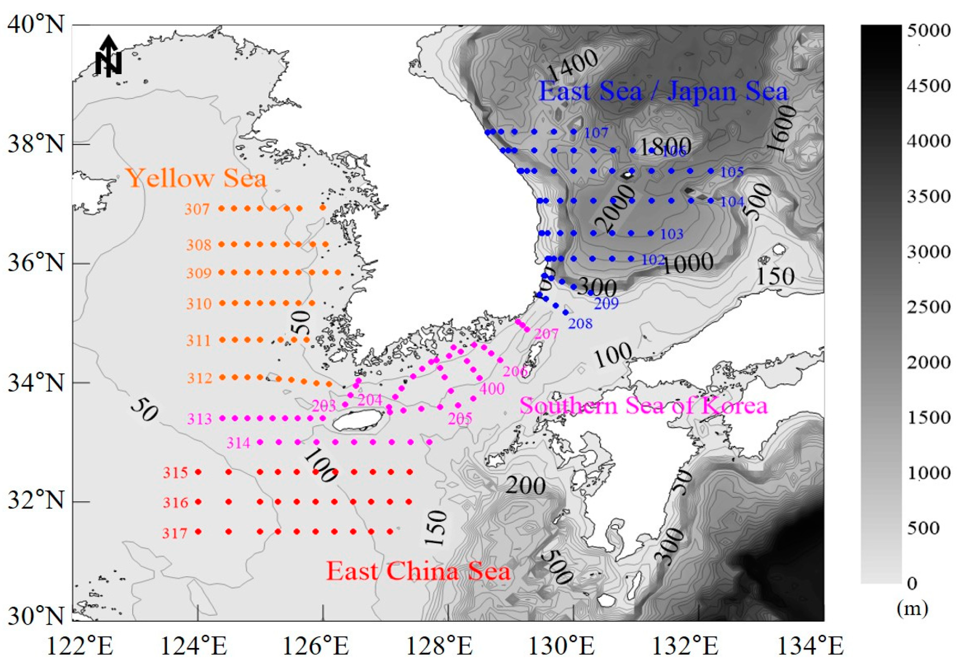
2.1. Study Area and Data Collection

To assess the characteristics of the water layers based on seawater density, we utilized oceanic data on water temperature and salinity obtained from the KODC (http://www.nifs.go.kr/kodc/soo_list.kodc, accessed on 22 May 2024). The KODC, operated by the National Institute of Fisheries Science (NIFS), has been collecting data to analyze the temperature trend around the Korean Peninsula due to climate change. The KODC provides standard depth-specific oceanographic variable data (e.g., temperature, salinity, and dissolved oxygen) at different water column depths (0, 10, 20, 30, 50, 75, 100, 125, 150, 200, 250, 300, 400, and 500 m) at 207 fixed stations along 25 oceanographic lines in the adjacent seas of Korea (124°–132°29′48.1″ E, 31°30′–38°12′36.0″ N) since the 1960s [6,11,12]. Among the KODC lines, we focused on data collected at 25 lines comprising 204 stations (East/Japan Sea: 69 stations, Southern Sea of Korea: 52 stations, Yellow Sea: 51 stations, East China Sea: 32 stations) classified by month and water layers and spanning from 1966 to 2021 (Figure 2).

The KODC assesses the quality of oceanographic data based on the standards of the Intergovernmental Oceanographic Commission (IOC) of UNESCO and assigns Quality Control flags (QC1–4, Quality Control) (

Table 1. Information of QC flags (NIFS, 2023). QC (Quality Control) represents the classification value to divide the levels of survey data.

QC Flag	Mean
QC1	Good
QC2	Not evaluated, not available or unknown
QC3	Questionable, suspect
QC4	Bad

).

Table 2. Number of water temperature data by QC flag in the adjacent seas of Korea (ES: East/Japan Sea; SS: Southern Sea of Korea; YS: Yellow Sea; ECS: East China Sea).

	ES	SS	YS	ECS	Sum
QC1	219,132	106,612	95,277	19,113	440,134
QC2	11,559	3032	2134	672	17,397
QC4	2	0	0	1	3
Sum	230,693	109,644	97,411	19,786	457,534

and

Table 3. Number of salinity data by QC flag in the adjacent seas of Korea (ES: East/Japan Sea; SS: Southern Sea of Korea; YS: Yellow Sea; ECS: East China Sea).

	ES	SS	YS	ECS	Sum
QC1	212,237	105,128	94,305	18,596	430,266
QC2	11,559	3032	2134	672	17,397
QC4	6897	1484	972	518	9871
Sum	230,693	109,644	97,411	19,786	457,534

present the number of water temperature and salinity of our used KODC data classified by quality level. The data volume for water temperature and salinity is the same in QC2, but salinity has a larger number of data than water temperature in QC4.

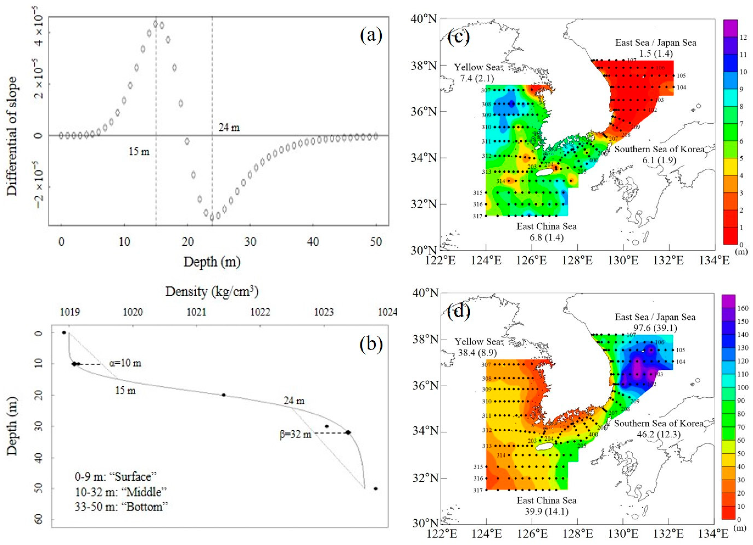
2.2. Water Layer Classification and Density Estimation

The vertical distribution of the ocean can be divided into three layers (surface layer, middle layer, and bottom layer) based on physical characteristics [13,14,15,16,17,18]. Among the oceanic environmental factors, the density of seawater is affected by changes in water temperature and salinity. Therefore, the pycnocline can be considered a factor that more reflects the physical characteristics of the ocean than the thermocline and halocline [19].

The August (summer) data, which exhibited clear classification by water layer, were used to evaluate oceanic characteristics for each water layer from 1966 to 2021 (Figure 3). Furthermore, by taking into account the water temperature and salinity data, the annual averaged water density at different depths was calculated using the equations and empirical constants proposed [19,20].

Oceanic water density typically increases with depth from the surface to the bottom, following an S-curve pattern [13,14]. Based on the pycnocline, which exhibits a rapid change in density, we classified the ocean into three layers: surface layer, middle layer, and bottom layer. Identifying density changes on a 1 m scale poses an important challenge due to the variations in depth-specific density evaluated by the KODC data exceeding 10 m. To address this limitation, we employed log-logistic regression, a nonlinear regression analysis method, to evaluate density changes at 1 m intervals. However, we excluded stations with fewer than three depth layers (stations 204-0, 205-0, and 308-1) from the analysis, as the data derived from these stations could not be subjected to the log-logistic regression. Additionally, we excluded station 105-15 (East/Japan Sea) due to its relatively limited annual data. Log-logistic regression analysis was performed using the ‘drm’ package in R (version 4.1.2).

To classify the water layer based on changes in the slope of depth-specific density, the depths of α and β were calculated for each observation station. The α was determined by applying linear regression analysis from the surface (0 m) to the depth where the slope of the log-logistic line changes from positive to negative (Figure 3a); α was defined as the point at which the density difference along the two regression lines for each depth was the largest (Figure 3b). The value of β was calculated using a similar process as for α, but starting from the maximum depth (Figure 3a,b). The surface layer (α > depth), middle layer (α ≤ depth ≤ β), and bottom layer (β < depth) were then defined based on the α and β values at the depth of the observation stations (Figure 3b).

2.3. Data Imputation and Statistical Analysis

Among the statistical imputation techniques for replacing the missing values, MI can be easily implemented using statistical software such as R and SAS [21,22,23]. MI has been widely applied to replace missing values in various fields, including agriculture, medicine, and behavioral ecology [22,23,24,25,26,27,28,29].

To enhance the quality of the original dataset, MI was applied to calibrate the QC2 and QC4 data of the water temperature and salinity variables, as shown in Table 1. QC2 and QC4 data are classified as data that have not been qualitatively verified or are not suitable for analysis.

Three statistical approaches were adopted in this study:

(1)

For data imputation, we considered three MI methods within the MICE framework: norm method, classification and regression trees (CART), and random forest (RF). The norm method is a simple imputation technique that does not consider predictor variables, which involves imputing missing values with the mean or median of the observed data. In contrast, both CART and RF are decision tree-based methods, which are particularly useful when the relationship between predictor variables and missing values is complex or nonlinear. To enhance the quality of the temperature and salinity data in QC2 and QC4, we assign the average value, repeating five times per MI methods (CART, RF, and the norm method), based on the QC1 data.

(2)

To estimate the distribution of density features, we considered several distributions and selected the best one from the data. The seven distributions considered in this study were the normal, skewed normal, log-normal, student T, log-gamma, gamma, and inverse gamma (inv-gamma) distributions. Each distribution has different assumptions and properties suitable for different types of data.

(3)

To select the best distribution, we compared the distribution from the imputed data with the distribution from the QC1field-observed data using the Kolmogorov–Smirnov (KS) test [30]. The KS test is a non-parametric statistical test that assesses the similarity between two probability distributions. This procedure helps determine if the two samples exhibit the same distribution or if there is a statistically significant difference between them. The KS test was used to identify the most suitable distribution for the target feature among the seven distributions. Afterward, the differences between the distributions of the new target feature and the original target feature were scored (

Table 4. Results of fitting distribution for ‘density’ features.

Area	Layer	Month
		2	4 (5)	6	8	10 (11)	12
East China Sea	bottom	log-gamma	log-gamma	-	gamma	log-gamma	-
	middle	log-gamma	log-gamma	-	log-gamma	log-gamma	-
	surface	log-gamma	log-gamma	-	skewed norm	log-gamma	-
East Sea	bottom	log-gamma	log-gamma	log-gamma	log-gamma	log-gamma	log-gamma
	middle	skewed norm	skewed norm	skewed norm	skewed norm	skewed norm	skewed norm
	surface	skewed norm	log-norm	skewed norm	student t	skewed norm	log-norm
Southern Sea of Korea	bottom	skewed norm	skewed norm	skewed norm	log-gamma	log-gamma	skewed norm
	middle	skewed norm	skewed norm	log-gamma	norm	log-norm	log-gamma
	surface	log-gamma	log-gamma	log-gamma	log-gamma	skewed norm	log-gamma
Yellow Sea	bottom	student t	skewed norm	log-gamma	log-gamma	log-gamma	log-norm
	middle	skewed norm	skewed norm	skewed norm	inv-gamma	skewed norm	skewed norm
	surface	skewed norm	skewed norm	skewed norm	skewed norm	skewed norm	log-gamma

).

2.4. Deep Learning-Based Time Series Analysis

Our proposed model consists of three deep learning-based processes: the trend model, the seasonality model, and the parametric process. First, the trend model consists of a series of piecewise regressions based on the change point to enable comparison with the long-term trend. The seasonality model includes Fourier terms to show regular fluctuations. As a result, this study proposes a parametric deep learning model that incorporates the uncertainty of water temperature through μ and σ² derived from the trend model and seasonality model.

Time series decomposition has the advantage of decomposing a time series into some components and combining the individual components to understand the pattern of the time series and predict the future value. Time series decomposition has an advantage in that independent components are linearly combined, so individual interpretation is possible and long-term trends can be expressed as a function of time like the generalized additive model [31,32]. In this study, water temperature (WT) was decomposed into two components: trend and seasonality.

For the sub-term trend model, the piecewise regression module (PWreg) transformed into a DL structure was used to decompose the change points and then connect them. As a result, when there are p change points, p + 1 regressions are used to combine them. The following is a more detailed formula:

$$\mathrm{P}\mathrm{W}\mathrm{r}\mathrm{e}\mathrm{g}\left(t\right)={\beta }_0+{\beta }_{1}t+\left(\begin{array}{ccc}\mathrm{h}\left(t_1-{cp}_1\right)& \dots & \mathrm{h}\left(t_1-{cp}_p\right)\\ \dots & \dots & \dots \\ \mathrm{h}\left(t_n-{cp}_1\right)& \dots & \mathrm{h}\left(t_n-{cp}_p\right)\end{array}\right)\times \left(\begin{array}{c}{\beta }_2\\ \dots \\ {\beta }_{p+1}\end{array}\right)$$

$$h\left(x\right)=\max \left(0,x\right)$$

Here, ${\beta }_0$ and ${\beta }_1$ are regression parameters of the before change points, ${cp}_p$ is the pth change point, and ${\beta }_{p+1}$ is the sub-term trend coefficient between ${cp}_p$ and ${cp}_{p+1}$.

We used Fourier transforms to model the seasonality components (Seasonality). A Fourier transform is the process of transforming a signal in the time domain into a signal in the frequency domain so that the entire signal can be described by the combination of a small number of Fourier terms. Fourier terms are used to represent the regular seasonality of a time series, and the appropriate number of Fourier terms needs to be determined. The following is the Fourier term formula:

$$\mathrm{S}\mathrm{e}\mathrm{a}\mathrm{s}\mathrm{o}\mathrm{n}\mathrm{a}\mathrm{l}\mathrm{i}\mathrm{t}\mathrm{y}\left(\mathrm{t}\right)={\sum }_{i=1}^s{f}_i\left(t\right)=a\times \cos \left({\displaystyle \frac{2\pi jt}{p}}\right)+b\times \mathrm{s}\mathrm{i}\mathrm{n}\left({\displaystyle \frac{2\pi jt}{p}}\right)$$

The mean squared error (MSE) is often used to measure the loss for training a regression model. MSE reduces the error through the sum of the squares of the differences between the predicted and actual values, but it has a limitation in that it cannot predict overfitting and uncertainty. Therefore, in this study, a parametric approach that includes uncertainty is proposed for learning a prediction model of water temperature. For this purpose, we used negative log-likelihood (NBLL) for the loss and assumed a normal distribution.

$$\mathrm{N}\mathrm{B}\mathrm{L}\mathrm{L}=-\log \left(p\left({WT}_n|t_n\right)\right)=0.5\times \log \left(2\pi {\sigma }^2\right)+0.5\times {\left({WT}_n-\mu \right)}^2/{\sigma }^2$$

$$\mu ={\mu }_T+{\mu }_S$$

Here, ${WT}_n$ is $n$th point of the water temperature, $t_n$ is the $n$th point, and ${\mu }_T$ and ${\mu }_S$ are the predicted means of trend and seasonality, respectively.

In our model, we designed the trend and seasonal components as explicit modules within a deep learning framework. PWreg learns segment-specific slopes and adjusts intercepts to ensure continuity across segments. Seasonality trains periodic behavior using learnable Fourier coefficients. All parameters are implemented as differentiable PyTorch 2.2.0 modules, enabling end-to-end learning via backpropagation. This modular design allows classical statistical structures to be reinterpreted and extended within a flexible and scalable deep learning architecture. For hyperparameter settings, we used a learning rate of 0.001 and a batch size of 16. Additionally, three Fourier transforms were applied to capture the seasonal components in the model.

3. Results and Discussion

3.1. Water Layer Classification

The estimated depths of α and β in the adjacent seas of Korea, which were used to classify the water layers, are illustrated in Figure 3c,d. The mean depth of α was deepest in the Yellow Sea (7.4 m), followed by the East China Sea (6.8 m), the Southern Sea of Korea (6.1 m), and the East/Japan Sea (1.5 m) (Figure 3c). The standard deviation of α was smallest in the East/Japan Sea and East China Sea, with little difference observed in the other two areas (Figure 3c). As for β, the mean depth was deepest in the East/Japan Sea (97.6 m), followed by the Southern Sea of Korea (46.2 m), the East China Sea (39.9 m), and the Yellow Sea (38.4 m) (Figure 3d). The standard deviation of β was largest in the East/Japan Sea, followed by the East China Sea, the Southern Sea of Korea, and the Yellow Sea (Figure 3d). The width of the middle layer (pycnocline, β-α) was widest in the East/Japan Sea (96.1 m), followed by the Southern Sea of Korea (40.1 m), the East China Sea (33.1 m), and the Yellow Sea (31 m). The depths of both α and β in ocean areas around the Korean Peninsula were influenced by the maximum depth, and the variation in β was larger than that in α as the ocean depth increased.

3.2. Data Imputation

To enhance the reliability of the analysis, the data quality was improved using imputation methods. Here, we proposed a novel distribution statistical approach that compares the similarity of the distribution of the target variable, rather than the existing method, to assess the imputation method’s performance. There was no statistically significant difference in the distribution of the actual density in 67% of the cases. Therefore, we introduced a new approach that considers the original target distribution to improve data quality.

The result of estimating distribution shows that most of the distributions are asymmetric, except for the ES surface in August and the YS bottom in February. In particular, log-gamma and skewed norm distribution account for the largest proportion. This can be interpreted in two ways. First, the KODC data are long-term data that have been observed for up to 56 years, which means that it may have a trend. Second, the normal distribution, which is bell-shaped and is commonly used in natural sciences, may not be suitable for marine data.

To compare the distribution of the original data and the reconstructed data using MI for each water layer, the data were evaluated separately on a two-month basis considering seasonality (three months for ECS). The null hypothesis (H₀) of the KS test assumes no difference between the density distribution of Q1 and the imputation density distribution. The number of cases where the null hypotheses was not rejected (

Table 5. Comparison of imputation methods using Kolmogorov–Smirnov (KS) test.

	CART	Norm	RF
# Not reject $H_0$ (total)	44 (66)	42 (66)	43 (66)
Percentage (%)	66.7	63.6	63.2

) indicated that the three methods, CART, Norm, and RF, demonstrated successful restoration in more than 60% of the cases (44, 42, and 43, respectively). Therefore, data imputation was conducted using the CART method. Additional comparisons of imputed data were shown in Figures S1 and S2.

Figure 4 illustrates the distribution of temperature in each sea. The temperature distribution in the Yellow Sea, Southern Sea of Korea, and East China Sea displayed similar patterns, with the highest water temperature distribution in summer and the lowest in winter. The deep areas exhibited lower water temperatures, resulting in some regions showing relatively low water temperatures during summer. The Yellow Sea had a lower water temperature distribution compared to other seas in summer due to the influence of the Yellow Sea Cold Bottom Water in the lower layer. The East/Japan Sea, on the other hand, exhibited the highest distribution of 0–5 °C temperature ranges as the East Sea Proper Water persisted throughout the year.

Next, trend comparisons were conducted using PWreg for the surface, middle, and bottom layers of the four seas (East/Japan Sea, Southern Sea of Korea, Yellow Sea, and East China Sea) around the Korean Peninsula. Change points of 2000 and 2009 were employed based on the years proposed in Refs. [10,33,34]. The results for the slope are presented in

Table 6. Results of trend changes for each layer of the four seas with two change points.

Area	Classification	Trend			Long-Term Trend [1966, 2021]
		[1966, 2000]	[2000, 2009]	[2009, 2021]
ECS	surface	0.226	−0.010	−0.096	0.013
ECS	middle	0.347	0.022	0.004	0.034
ECS	bottom	0.232	−0.059	−0.017	0.040
ES	surface	0.060	−0.075	0.170	0.036
ES	middle	0.044	0.020	0.067	0.027
ES	bottom	−0.036	0.031	0.043	−0.026
YS	surface	0.049	0.015	−0.003	0.021
YS	middle	0.046	0.004	0.200	0.016
YS	bottom	0.021	−0.004	−0.017	0.000
SS	surface	0.052	−0.079	−0.048	0.015
SS	middle	0.035	−0.131	0.118	0.010
SS	bottom	0.034	−0.048	0.062	0.007

.

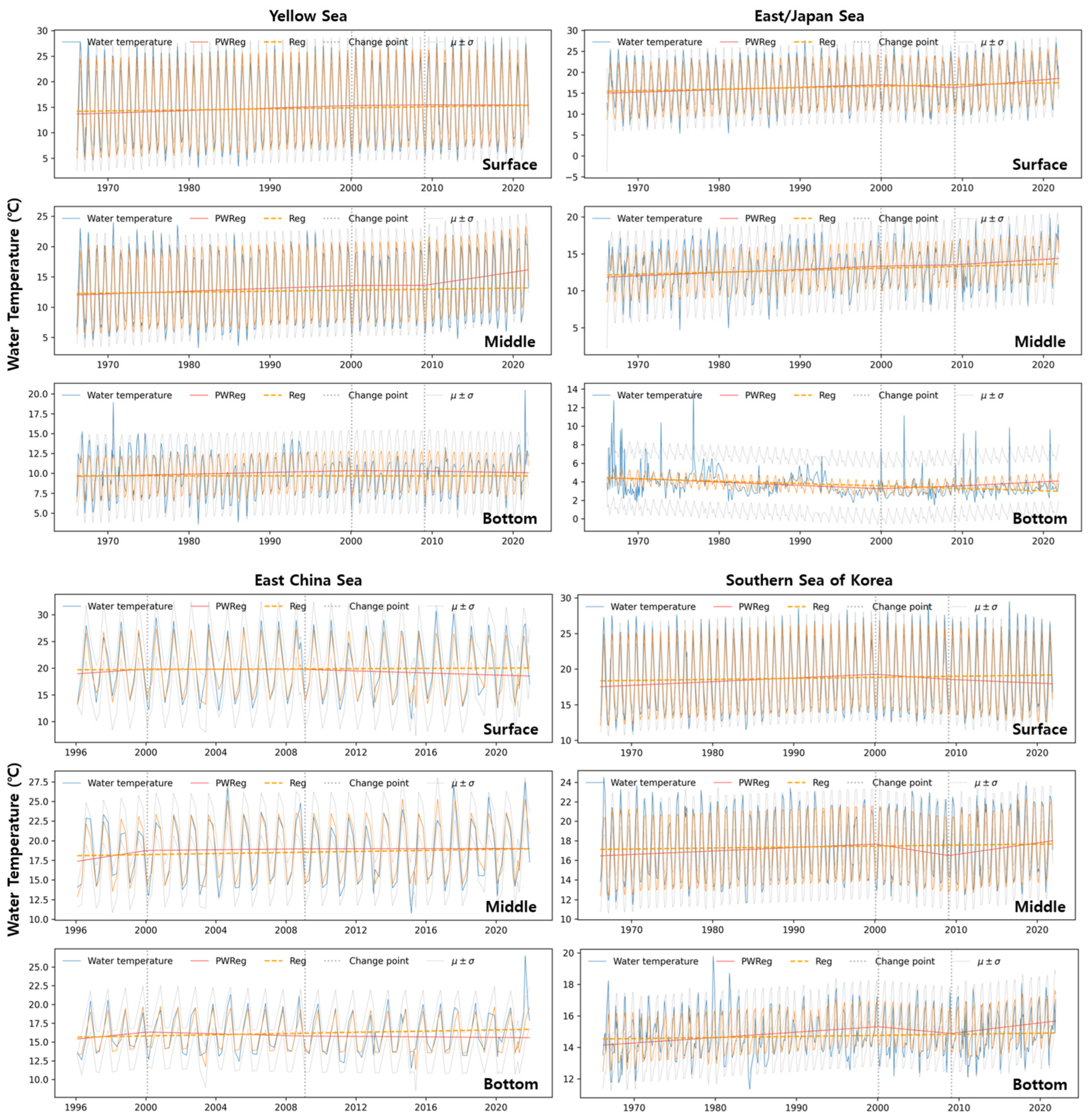
3.3. Temperature Trends

Ref. [33] reported a slowdown in global warming since 2000, whereas Ref. [34] observed the opposite trend in the long-term water temperature trend in the Yellow Sea region starting from 2000. Ref. [10] analyzed the water temperature trend around the Korean Peninsula using KODC data and noted a rapid rise in water temperature trends since 2009. Hence, in this study, the long-term water temperature trend was analyzed by selecting 2000 and 2009 as the inflection points.

The characteristics of the proposed model are shown in Figure 5. We predicted trend, seasonality, and even variance with the end-to-end model, but we used linear combination, which allows for separate interpretations of PWReg and Seasonality. For example, Figure 5a. compares the trend using PWReg and the long-term using regression. And by adding seasonality, a more accurate fitting is possible (Figure 5b). Finally, the estimated variance can be used to evaluate anomalous water temperatures with confidence intervals (Figure 5c). The detailed algorithm is shown in the Supplementary Materials.

The water temperature trends for each layer in the different sea areas are presented in Table 6 and Figure 6. Data for all sea areas have been available since 1966; however, data for the East China Sea have only been available since 1996. Therefore, the analysis for the East China Sea was conducted from 1996 onward.

Prior to 2000, most water temperature trends exhibited positive values, except for the bottom layer of the East/Japan Sea. Notably, the middle layer of the East China Sea exhibited the highest temperature trend of 0.347 °C/year, whereas the surface layer of the East China Sea followed with 0.226 °C/year. In the East China Sea, the water temperature increased the most in the middle layer, followed by the bottom and surface layers. In the East/Japan Sea, the water temperature rose in the surface (0.06 °C/year) and middle layers (0.044 °C/year) but decreased in the bottom layer (−0.036 °C/year). The Yellow Sea showed a small increase in the surface (0.049 °C/year) and middle layers (0.046 °C/year), while the bottom layer also exhibited a positive trend (0.021 °C/year). Similarly, in the Southern Sea, all layers showed a rising trend, with the surface layer (0.052 °C/year) experiencing the highest increase. In terms of spatial distribution, most of the surface layers exhibited an increasing trend, whereas the bottom layer of the East/Japan Sea displayed a downward trend.

From 2000 to 2009, a period that coincided with a slowdown in global warming, most layers showed negative trends, except for the middle and bottom layers of the East/Japan Sea and the surface and middle layers of the Yellow Sea. The surface layer of the East China Sea exhibited the lowest value of −0.010 °C/year. The positive trend in the Yellow Sea was somewhat consistent with the findings of Ref. [33], whereas the decrease in the Southern Sea’s middle layer (−0.131 °C/year) was significant.

Since 2009, all study areas in the middle layer have shown a positive trend, with values larger than in other periods except the East China Sea, indicating a rapid rise in water temperature. The middle layer of the Yellow Sea exhibited the highest water temperature trend at 0.200 °C/year, whereas the lowest trend was observed in the bottom layer of the Yellow Sea (−0.017 °C/year). Strongly rising water temperature trends were evident in all layers of the East/Japan Sea, especially in the surface layer (0.170 °C/year).

The overall water temperature trend over the entire period exhibited positive values, except for the bottom layer of the East/Japan Sea (−0.026 °C/year) and the bottom layer of the Yellow Sea (0.000 °C/year). The decrease in water temperature in the lower layers of the East/Japan Sea and the Yellow Sea suggests the influence of stratification due to weakening winds. When wind currents are weak, vertical mixing is reduced, leading to stronger stratification and a greater difference between surface and lower water temperatures. Therefore, as the wind gradually weakens, surface water temperatures rise while bottom water temperatures decrease. Ref. [6] reported that the surface water temperature of the East/Japan Sea increased in winter, which coincided with an increase in the associated temperature and a weakened wind speed. As a result, winters have become gradually warmer with weakened winds. In this study, the increase in surface water temperature and the decrease in bottom water temperature in the East/Japan Sea were likely strongly influenced by wind.

3.4. Influence of Pacific Decadal Oscillation

We analyzed the Pacific Decadal Oscillation (PDO) index, which is closely related to climate change, in conjunction with sea surface temperatures (SSTs) around the Korean Peninsula (Figure 7). A cross-correlation analysis was conducted to determine the time lag between the PDO index and the SST. To eliminate seasonal variations, the monthly mean values were subtracted from both the PDO and SST data. The results showed no time lag in the Yellow Sea and the East Sea, whereas the South Sea exhibited an 8-month lead. However, as all correlation coefficients (R values) were below 0.05, the relationship between the PDO index and SST around the Korean Peninsula was found to be insignificant.

One possible explanation is that localized oceanographic processes, such as the East Korea Warm Current and variations in the Yellow Sea Cold Bottom Water, play a more dominant role in modulating temperature trends in this region. Additionally, weakening monsoon wind intensity and changes in vertical mixing may have contributed to the observed trends, reinforcing the importance of considering regional climate dynamics in ocean temperature studies.

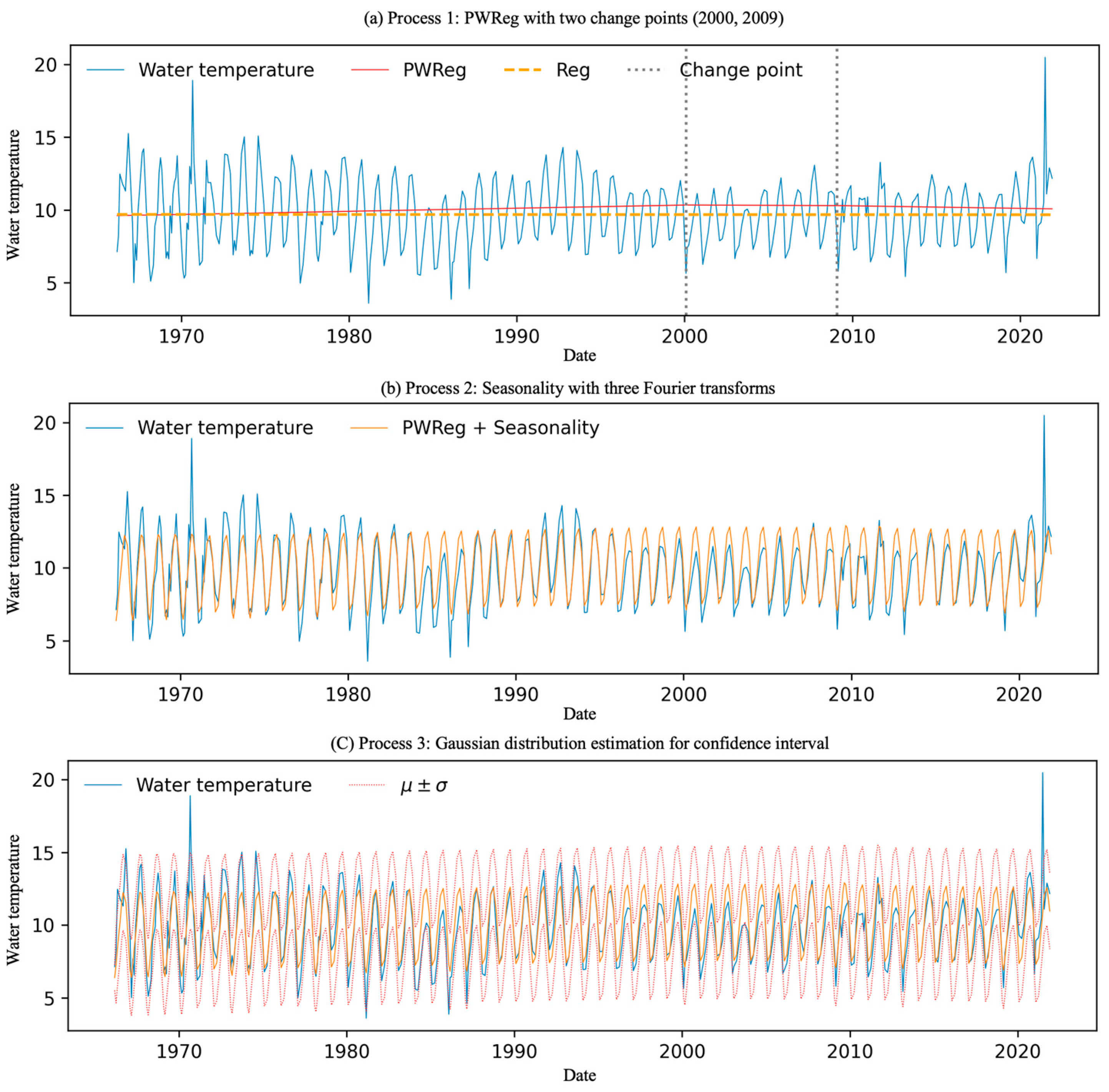
3.5. Proposed Model for Long-Term Temperature Analysis

The main objective of this study is to analyze the long-term evolution of ocean temperatures, not simply to predict future values. To this end, we incorporated both trend and seasonality components into the model [35,36]. To analyze structural changes in the long-term trend, we used PWReg, which allowed us to quantitatively assess the impact of climate change at key inflection points (e.g., 2000 and 2009). By applying separate regression models at different time points, PWReg effectively detects and learns abrupt changes in the data to provide interpretable trend estimates.

In addition to trend modeling, seasonality was incorporated using Fourier trans-form, which decomposes the periodic fluctuations in water temperature into frequency components. By selecting the appropriate number of Fourier terms, the model effectively captures the regular seasonal variations in ocean temperature, providing a more comprehensive representation of temperature dynamics compared to traditional regression-based approaches. This improves interpretability and allows for an accurate representation of both long-term trends and cyclical fluctuations.

It also adopts a parametric approach that assumes a Gaussian distribution to estimate uncertainty in water temperature forecasts. Unlike traditional deterministic models, this approach provides confidence intervals that quantify the confidence of the forecast. By using the negative log-likelihood (NLL) as the loss function, our model explicitly accounts for uncertainty, making it more robust to changes in ocean conditions. This probabilistic framework not only improves forecast performance but also increases the interpretability of model results by providing uncertainty estimates alongside point forecasts.

By incorporating partial regression for trend detection, Fourier transform for seasonality modeling, and a Gaussian-based parametric framework for uncertainty estimation, the proposed model balances interpretability with forecast accuracy. This flexible structure allows for further refinement of climate impact assessments in the future, such as incorporating additional oceanographic variables.

4. Conclusions

In this study, we proposed a systematic approach to analyzing NIFS ocean observation data by disaggregating the data into three layers. To ensure the reliability of the reconstructed data, we implemented and rigorously validated an estimation strategy using statistical methods. Using these estimated long-term datasets, we comprehensively analyzed water temperature changes in different layers surrounding the Korean Peninsula, providing new insights into long-term oceanographic trends. Water density was calculated using NIFS water temperature and salinity data. The log-logistic method was used to divide the density data by depth in August into three vertical layers (surface, middle, and bottom layers). Low-quality data (QC2 and QC4) in the original dataset were generated using the CART method, a machine learning technique. Next, we introduced a statistical approach to evaluate imputation methods by considering invariance to the target, thus avoiding limitations observed in mean or median value replacement methods (e.g., overestimation of mean values when there are fewer data) and improving the representation of target characteristics through statistical testing.

Furthermore, we proposed a DL-based Gaussian distribution model, including PWReg and seasonality, that offers significant advantages over traditional deterministic models. Unlike traditional regression methods that only provide point estimates, this approach allows us to quantify uncertainty through confidence intervals. By incorporating a probabilistic framework, we can assess the confidence of predictions and account for variability in sea temperature trends. This is particularly useful for climate research, where understanding uncertainty is essential for robust decision making and long-term forecasting.

References

1. Arias, P.; Bellouin, N.; Coppola, E.; Jones, R.; Krinner, G.; Marotzke, J.; Naik, V.; Palmer, M.; Plattner, G.; Rogelj, J. Climate Change 2021: The Physical Science Basis. Contribution of Working Group I to the Sixth Assessment Report of the Intergovernmental Panel on Climate Change; Technical Summary; Cambridge University Press: Cambridge, UK, 2021. [Google Scholar]
2. Nakao, T. Oceanic variability in relation to fisheries in the East China Sea and the Yellow Sea. J. Fac. Mar. Sci. Technol. Tokai Univ. 1977, 199–367. [Google Scholar]
3. Park, K.; Park, J.; Choi, B.; Lee, S.; Shin, H.; Lee, S.; Byun, D.; Kang, B.; Lee, E. Schematic maps of ocean currents in the Yellow Sea and the East China Sea for science textbooks based on scientific knowledge from oceanic measurements. J. Korean Soc. Oceanogr. 2017, 22, 151–171. [Google Scholar] [CrossRef]
4. Chen, C.; Xue, P.; Ding, P.; Beardsley, R.C.; Xu, Q.; Mao, X.; Gao, G.; Qi, J.; Li, C.; Lin, H. Physical mechanisms for the offshore detachment of the Changjiang Diluted Water in the East China Sea. J. Geophys. Res. Ocean. 2008, 113, C2. [Google Scholar] [CrossRef]
5. Park, M.; Song, J.; Han, I.; Lee, J. A Study of Long-term Trends of SST in the Korean Seas by Reconstructing Historical Oceanic Data. J. Korean Soc. Mar. Environ. Saf. 2019, 25, 881–897. [Google Scholar] [CrossRef]
6. Seong, K.; Hwang, J.; Han, I.; Go, W.; Suh, Y.; Lee, J. Characteristic for long-term trends of temperature in the Korean waters. J. Korean Soc. Mar. Environ. Saf. 2010, 16, 353–360. [Google Scholar]
7. Yoon, S.C.; Youn, S.H.; Shim, M.J.; Yoon, Y.Y. Characteristics and variation trend of water mass in offshore of the east coast of Korea during last 10 years. J. Korean Soc. Mar. Environ. Energy 2017, 20, 193–199. [Google Scholar] [CrossRef]
8. Ghahramani, Z.; Michael, I.J. Supervised learning from incomplete data via an EM approach. Adv. Neural Inf. Process Syst. 1994, 6, 120–127. [Google Scholar]
9. Beckers, J.-M.; Michel, R. EOF Calculations and Data Filling from Incomplete Oceanographic Datasets. J. Atmos. Ocean. Technol. 2003, 20, 1839–1856. [Google Scholar] [CrossRef]
10. Han, I.; Lee, J. Change the annual amplitude of sea surface temperature due to climate change in a recent decade around the Korean Peninsula. J. Korean Soc. Mar. Environ. Saf. 2020, 26, 233–241. [Google Scholar] [CrossRef]
11. Han, S.-B. Hydrographic Observations around Korean Peninsula: Past, Present and Future. J. Korean Soc. Oceanogr. 1992, 27, 332–341. [Google Scholar]
12. Korea Oceanographic Data Center. Available online: https://www.nifs.go.kr/kodc/soo_list.kodc (accessed on 10 April 2023).
13. Kara, A.B.; Rochford, P.A.; Hurlburt, H.E. Mixed layer depth variability over the global ocean. J. Geophys. Res. Ocean. 2003, 108, C3. [Google Scholar] [CrossRef]
14. Kara, A.B.; Rochford, P.A.; Hurlburt, H.E. An optimal definition for ocean mixed layer depth. J. Geophys. Res. Ocean. 2000, 105, 16803–16821. [Google Scholar] [CrossRef]
15. Yoon, D.; Choi, H. Development of algorithms for extracting thermocline parameters in the South Sea of Korea. Ocean. Polar Res. 2012, 34, 265–273. [Google Scholar] [CrossRef]
16. Ryu, I.; Lee, B.; Cho, Y.; Choi, H.; Shin, D.; Kim, S.; Yu, S. Analyzing Flow Variation and Stratification of Paldang Reservoir Using High-frequency W ater Temperature Data. J. Korean Soc. Water Environ. 2020, 36, 392–404. [Google Scholar] [CrossRef]
17. Kim, K.; Kim, K.; Kim, Y.; Cho, Y.; Kang, D.; Takematsu, M.; Volkov, Y. Water masses and decadal variability in the East Sea (Sea of Japan). Prog. Oceanogr. 2004, 61, 157–174. [Google Scholar] [CrossRef]
18. Kim, Y.O.; Choi, J.; Choi, D.H.; Oh, K. A biological indication of vertical mixing of the Yellow Sea Bottom Cold Water. Ocean. Sci. J. 2023, 58, 7. [Google Scholar] [CrossRef]
19. Lee, W.; Hur, D. Development of 3-d hydrodynamical model for understanding numerical analysis of density current due to salinity and temperature and its verification. KSCE J. Civ. Eng. 2014, 34, 859–871. [Google Scholar] [CrossRef]
20. Gill, A.E. Transfer of Properties between Atmosphere and Ocean. In Atmosphere—Ocean Dynamics; Academic Press: New York, NY, USA, 1982; pp. 36–38. ISBN 0122835204. [Google Scholar]
21. Zhang, Z. Multiple imputation with multivariate imputation by chained equation (MICE) package. Ann. Transl. Med. 2016, 4, 30. [Google Scholar] [CrossRef]
22. Yuan, Y. Multiple imputation using SAS software. J. Stat. Softw. 2011, 45, 1–25. [Google Scholar] [CrossRef]
23. Murray, J.S. Multiple imputation: A review of practical and theoretical findings. Statist. Sci. 2018, 33, 142–159. [Google Scholar] [CrossRef]
24. Kim, H.; Soh, H.Y.; Kwak, M.; Han, S. Machine learning and multiple imputation approach to predict chlorophyll-a concentration in the coastal zone of Korea. Water 2022, 14, 1862. [Google Scholar] [CrossRef]
25. Sheng, H.; Liu, H.; Wang, C.; Guo, H.; Liu, Y.; Yang, Y. Analysis of cyanobacteria bloom in the Waihai part of Dianchi Lake, China. Ecol. Inf. 2012, 10, 37–48. [Google Scholar] [CrossRef]
26. Sterne, J.A.; White, I.R.; Carlin, J.B.; Spratt, M.; Royston, P.; Kenward, M.G.; Wood, A.M.; Carpenter, J.R. Multiple imputation for missing data in epidemiological and clinical research: Potential and pitfalls. BMJ 2009, 338, b2393. [Google Scholar] [CrossRef]
27. Nakagawa, S.; Freckleton, R.P. Model averaging, missing data and multiple imputation: A case study for behavioural ecology. Behav. Ecol. Sociobiol. 2011, 65, 103–116. [Google Scholar] [CrossRef]
28. Mackinnon, A. The use and reporting of multiple imputation in medical research—A review. J. Intern. Med. 2010, 268, 586–593. [Google Scholar] [CrossRef]
29. Lokupitiya, R.S.; Lokupitiya, E.; Paustian, K. Comparison of missing value imputation methods for crop yield data. Environmetrics 2006, 17, 339–349. [Google Scholar] [CrossRef]
30. Berger, V.W.; Zhou, Y. Kolmogorov–smirnov test: Overview. In Wiley Statsref: Statistics Reference Online; John Wiley & Sons Press: New York, NY, USA, 2014; pp. 1–5. [Google Scholar] [CrossRef]
31. Hwang, K.; Jung, S. Decadal changes in fish assemblages in waters near the Ieodo ocean research station (East China Sea) in relation to climate change from 1984 to 2010. Ocean Sci. J. 2012, 47, 83–94. [Google Scholar] [CrossRef]
32. Yoon, S.; Chang, K.; Na, H.; Minobe, S. An east-west contrast of upper ocean heat content variation south of the subpolar front in the East/Japan Sea. J. Geophys. Res. Ocean. 2016, 121, 6418–6443. [Google Scholar] [CrossRef]
33. Rahmstorf, S.; Foster, G.; Cahill, N. Global temperature evolution: Recent trends and some pitfalls. Environ. Res. Lett. 2017, 12, 054001. [Google Scholar] [CrossRef]
34. Lee, E.; Park, K. Validation of satellite sea surface temperatures and long-term trends in Korean coastal regions over past decades (1982–2018). Remote Sens. 2020, 12, 3742. [Google Scholar] [CrossRef]
35. Taylor, S.J.; Letham, B. Forecasting at scale. Am. Stat. 2018, 72, 37–45. [Google Scholar] [CrossRef]
36. Triebe, O.; Laptev, N.; Rajagopal, R. NeuralProphet: Explainable Forecasting at Scale. arXiv 2021, arXiv:2111.15397. [Google Scholar] [CrossRef]
Figure 1. Overall model process. PWreg = piecewise regression module.
Water 17 01066 g001
Figure 2. Study areas and data collected at stations in the adjacent seas of Korea. The dots represent the KODC line-stations of the National Institute of Fisheries Science, whereas the contour lines indicate the depth.
Water 17 01066 g002
Figure 3. (a) Changes in water density gradient by depth and (b) estimation of α and β to classify the water layers by considering the changes in the slope of depth-specific density at station 317-17 in the East China Sea. Depths of were α (c) and β (d) evaluated to classify the water layer using August data from 1966 to 2021 in the adjacent seas of Korea. The values below the area indicate the mean and standard deviation (values in parentheses), respectively.
Water 17 01066 g003
Figure 4. Distribution of temperature in each sea. ES, SS, YS, and ECS represent East/Japan Sea, Southern Sea of Korea, Yellow Sea, and East China Sea. The numbers in each sea are observed month.
Water 17 01066 g004
Figure 5. Proposed model components for long-term water temperature analysis at bottom layer in the Yellow Sea. (a) Piecewise regression module (PWReg) with two change points (2000, 2009). The water temperature time series (blue) is segmented using change points (dotted lines), with PWReg capturing trend shifts (red line). Orange line means regression (Reg) for long-term trend. (b) Seasonal modeling with three Fourier terms. The Fourier-based seasonality model (orange) captures periodic fluctuations in water temperature. (c) Gaussian distribution-based uncertainty estimation. The estimated mean (μ, orange) and variance (σ2, dotted red) provide confidence intervals, allowing uncertainty quantification.
Water 17 01066 g005
Figure 6. Proposed model components for long-term water temperature analysis in all seas.
Water 17 01066 g006
Figure 7. PDO index with regression and PWReg. Red and green lines represent regression and PWReg, respectively.
Water 17 01066 g007