Forecasting Evaporation Trends Amid Climate Change for Sustainable Water Management in Semi-Arid Regions

Abstract

Evapotranspiration plays a vital role in the design of irrigation systems, water resource management, and hydrological modeling, especially in arid and semi-arid regions. This study focuses on projecting evaporation rates using three machine learning models: a Support Vector Machine (SVM), Multi-Layer Perceptron (MLP), and Gaussian Process Regression (GPR), in combination with Principal Component Analysis (PCA) for dimensionality reduction. Meteorological data from 1980 to 2022, including the minimum and maximum temperatures, rainfall, and solar radiation, were used to train and test the models. Projections were made for Kirkuk Governorate by downscaling five global climate models under two climate scenarios: SSP2-4.5 and SSP5-8.5. These scenarios were used to predict future evaporation rates at a rainwater harvesting site for four future periods (P1, P2, P3, and P4) and compare them to the historical reference period (RP). The performance of the models was evaluated using three statistical metrics: Mean Absolute Error (MAE), Root Mean Squared Error (RMSE), and the regression coefficient (R²). Among the models, the MLP demonstrated superior predictive accuracy, with values of MAE = 0.02 mm, RMSE = 0.10 mm, and R² = 0.95. The SVM model showed a slightly lower performance, with MAE = 0.21 mm, RMSE = 0.13 mm, and R² = 0.92. The GPR model’s performance was comparable, yielding MAE = 0.22 mm, RMSE = 0.37 mm, and R² = 0.91. The historical reference period (RP) showed an average evaporation rate of 1370.9 mm per year. Under the SSP2-4.5 scenario, evaporation is projected to increase by 57.2%, while under SSP5-8.5, the increase is projected to be 85.9%. Under the SSP2-4.5 scenario, the evaporation rate for period P1 (2031–2050) showed a slight increase of 1.61%, while for periods P2 (2051–2070) and P3 (2071–2090), the increases were smaller, at 1.89% and 1.93%, respectively. The highest increase occurred in P4 (2091–2100), with a rate of 2.68%, compared to an observed value increase of 1.33%. These findings suggest that climate change will significantly elevate evaporation rates in the region, emphasizing the need for adaptive water resource management strategies.

1. Introduction

Reference Evapotranspiration hereinafter referred to as evaporation plays a critical role in the hydrological cycle, where water transforms from liquid to vapor through heat energy input. Managing limited water resources sustainably, especially amidst rapid population growth, is increasingly crucial for agricultural production [1]. Evaporation uses up a large amount of the water supplies accessible in hot regions by contributing considerably to water loss from rivers, canals, and open-water bodies. Even in humid areas, evaporation is still important, albeit accumulating precipitation, especially during rainy seasons, may dominate it. Additionally, the rate of evaporation plays a crucial role in understanding climate change and global warming, as it accounts for a significant portion of global precipitation loss [2].

Understanding the magnitude and variability of evaporation losses is essential for designing and managing water resources effectively [3]. Reliable models are necessary to quantify these losses accurately, especially as water resources become scarcer. Water resource development projects and irrigation systems rely heavily on long-term average values of evaporation for their design and operation [4]. As a result, an accurate evaporation calculation is essential to guaranteeing the sustainable and effective management of water resources. In addition to machine learning-based models, another widely used approach for measuring evaporation is the Penman evaporation equation, which combines energy balance and aerodynamic principles to estimate evaporation from a surface. This method accounts for factors such as the temperature, solar radiation, wind speed, and humidity. A recent study by [5] applied the Penman equation in the context of rainwater harvesting systems for ablution purposes, highlighting its feasibility and accuracy in predicting evaporation rates.

Evaporation rates are affected by various meteorological factors, such as maximum and minimum temperatures, sunshine duration or solar radiation, wind speed, relative humidity, rainfall, and vapor pressure, which are specific to each location [6]. However, continuously and accurately measuring pan evaporation is difficult. In these cases, stochastic or neural network models are vital for estimating pan evaporation from available climatic data, often producing more reliable results than direct measurements [7]. Since a direct evaporation measurement using evaporation pans is costly and inconvenient due to the experimental setup and logistical issues, evaporation is typically estimated through regression-based methods or other parametric models like Empirical Evaporation Equations, as well as the Water-Budget and Energy-Budget methods [8].

Researchers have developed various models for predicting evaporation pan evaporation across different locations in this globe. Numerous evaporation forecasting techniques currently in use are based on empirical correlations derived from climatological parameters or deterministic principles, such as the integrated energy balance-vapor transfer approach. These approaches often require rigorous local calibration, which limits their applicability on a global scale [9]. To recognize these limitations, there is a growing need to enhance conventional modeling techniques to achieve a better performance by adopting new and advanced methods.

Evaporation is a complex process characterized by non-linear behavior, making it suitable for modeling using Artificial Neural Networks (ANNs). To anticipate evaporation data, artificial intelligence (AI) methods like support vector machines (SVM) and artificial neural networks (ANN) have been widely and successfully applied. A major benefit of these AI methods is their nonparametric nature, meaning they do not require prior knowledge of the relationships between input variables and output data. ANNs are capable of capturing complex patterns and relationships in data, which traditional methods may find difficult to handle [10]. By leveraging ANNs, researchers aim to improve the accuracy and robustness of evaporation predictions across diverse geographical and climatic conditions. In summary, the evolution towards advanced modeling techniques like ANNs is driven by the desire to overcome the limitations of existing models, enhance the predictive accuracy, and enable the more effective management of water resources impacted by evaporation [11].

Numerous researchers have developed various models using Artificial Neural Networks to predict pan evaporation in different regions around the world. For instance, Al-Sudan and Saleem [7] demonstrated in their study the evaporation prediction by using machine learning techniques in Diyala in Iraq by using different models with five input variables; the results showed a prediction enhancement in terms of MAE and RMSE by 7.17% and 21.01%, 16.51% and 15.74%, and 23.14% and 26.64%, respectively. While Gohrbani et al. [12] utilized a hybrid model of an artificial neural network to predict pan evaporation in northern Iran as a semi-arid region, the results show that an optimal MLP-FFA model outperforms the MLP and SVM model for both tested stations. For Talesh, a value of WI = 0.926, NS = 0.791, and RMSE = 1.007 mm day⁻¹ is obtained using the MLP-FFA model, compared with 0.912, 0.713, and 1.181 mm day⁻¹ (MLP) and 0.916, 0.726, and 1.153 mm day⁻¹ (SVM), whereas for Manjil, a value of WI = 0.976, NS = 0.922, and 1.406 mm day⁻¹ is attained that contrasts 0.972, 0.901, and 1.583 mm day⁻¹ (MLP) and 0.971, 0.893, and 1.646 mm day⁻¹ (SVM). Hamza [13] used an artificial neural network to predict evaporation in the southern region of Iraq in Basrah as a semi-arid region and he used four input variables (temperature, rainfall, sunshine hours, and wind speed).

Konapala et al. [1] examined seasonal hydro-climate regimes using a non-parametric analysis methodology. They assessed changes in the water availability brought on by simultaneous changes in the mean and seasonal precipitation and evaporation using precipitation and evaporation. Rai et al. [14] used support vector machines, random forest approaches, multiple linear regression, multivariate adaptive regression splines, and weekly pan evaporation modeling. 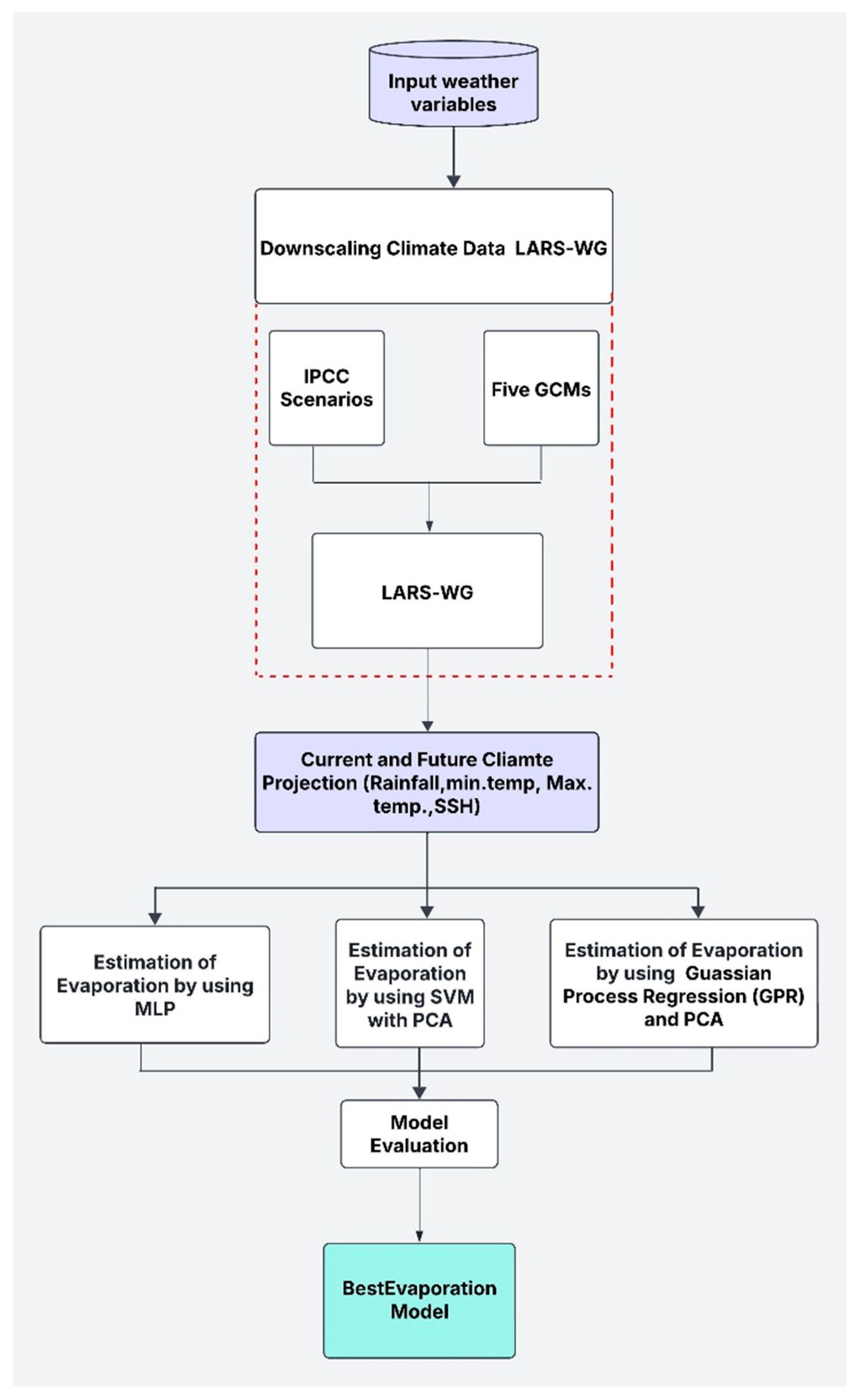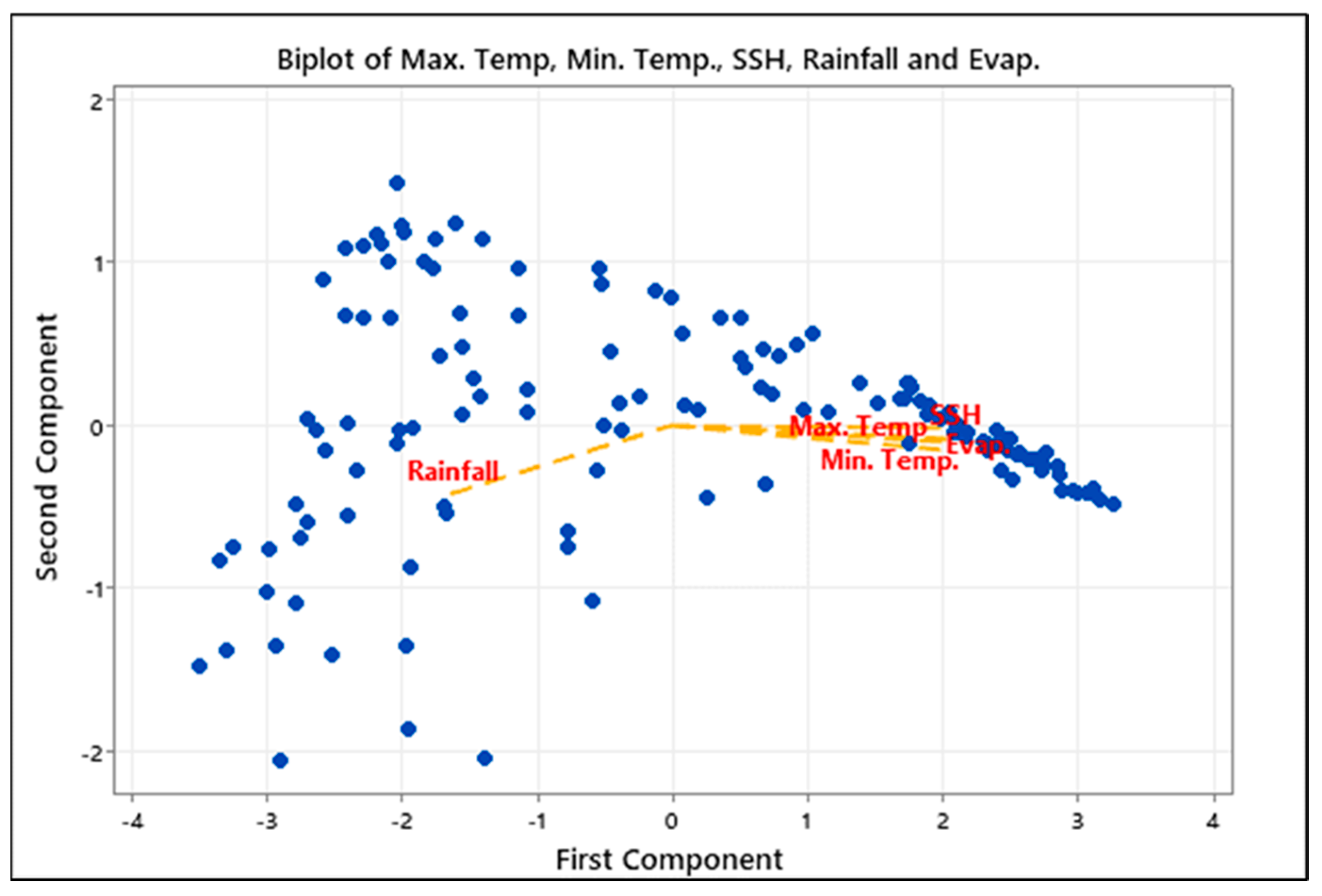Statistical metrics including the coefficient of determination (R²), the Nash–Sutcliffe coefficient of efficiency (NSE), and root mean square error (RMSE) were used to assess the efficacy of weekly pan-evaporation-estimating models for the Ranichauri station, which is situated in Uttarakhand, India’s Mid-Himalayan area. Both under- and over-predicted outcomes can be seen in the weekly pan evaporation values. However, all these researchers utilized the pan evaporation prediction in different locations, but none of these studies utilized the evaporation prediction under the impact of climate change and a future projection. This study presents an original approach by employing and comparing three advanced machine learning models—a Multi-Layer Perceptron (MLP), Support Vector Machine (SVM), and Gaussian Process Regression (GPR)—which are integrated with climate projections and climatic scenarios. A unique aspect of this research is the incorporation of Principal Component Analysis (PCA) for dimensionality reduction, enhancing the accuracy and performance of the models. Principal Component Analysis (PCA) and Linear Discriminant Analysis (LDA) are both widely used dimensionality reduction techniques, but they differ significantly in their approach and objectives. PCA is an unsupervised technique, meaning it does not take into account any class labels when reducing dimensions. It aims to maximize the variance in the data by identifying principal components in orthogonal directions in which the data vary the most. PCA is particularly useful when the goal is to capture as much information (variance) as possible from the original dataset, irrespective of any classification or group membership. This study leverages five global climate models under two significant climate scenarios: Shared Socioeconomic Pathways (SSP2-4.5 and SSP5-8.5), providing a robust analysis of the potential impacts of climate change. The research focuses on the semi-arid region of Kirkuk, in northern Iraq, to predict evaporation rates under changing climate conditions, which has critical implications for water resource management in such vulnerable environments.

The comparative analysis of three sophisticated models (MLP, SVM, and GPR), in combination for this application with the integration of PCA with these models, improves the model efficiency and highlights the most important features influencing evaporation. The application of this advanced methodology integrated under two climate scenarios (SSP2-4.5 and SSP5-8.5) is specific to a semi-arid, climate-sensitive region (Kirkuk), offering valuable insights into climate change impacts on evaporation in arid environments. The main aim of this study is to predict evaporation under the impact of climate change by developing multiple models including MLP, SVM with PCA, and GPR with PCA under the impact of climate change and GCMs, and comparing these models and choosing the best model for the evaporation prediction. This paper is organized as follows: Section 2 includes the climatic data and study region, then Section 3 illustrates the methodology, Section 4 the results and discussion, and finally, Section 5 includes the conclusion.

2. Climatic Data and Study Region

2.1. Study Region

The Kirkuk Governorate is located in northern Iraq, bordered to the northeast by the Zagros Mountains and to the west by the Lower Zab and Tigris Rivers, known for their gentle flow. Kirkuk lies about 250 km (155 miles) from Baghdad, the capital and largest city of Iraq. The study area is situated between latitudes 35°28′ N and 35°47′ N, and longitudes 44°24′ E and 44°40′ E, at an elevation of 350 m. The northeastern highlands of Iraq begin in southern Kirkuk and stretch toward the borders of Turkey and Iran. Kirkuk is divided into three distinct neighborhoods: Daquq, Al-Hawiga, and Dibis. Despite its relatively small size, the governorate spans approximately 9679 square kilometers, representing around 2.2% of Iraq’s total land area. Kirkuk holds significant importance in agriculture [15]. According to Iraqi government estimates in 2007, Kirkuk’s population was about 902,019, making up roughly 3% of Iraq’s total population.

2.2. Climatic Data

The climate in the Kirkuk Governorate ranges from semi-arid to Mediterranean, characterized by warm summers and cold, rainy winters. The region experiences four distinct seasons, with winter lasting from December to the end of February. During this time, the weather is relatively mild to cool, with average daytime temperatures ranging between 10 °C and 15 °C, though night-time temperatures can occasionally drop close to freezing. The spring season lasts from March to May, and it is mild with average temperature ranging from 16 °C to 25 °C; it is also one of the wetter seasons. Meanwhile, the summer season is from June to September; it is hot and dry, often with temperatures exceeding 40 C during the hottest months (July and August) and there is no rainfall during these months. The autumn in Kirkuk is from October to November and is mild, and the temperature starts to drop down and rainfall begins to increase during this time.

The rainfall season is mainly in winter through spring in the Kirkuk Governorate and the average annual rainfall varies from 300–400 mm.

Table 1. Average values for main climatic data.

Months	Av. Tmax. (°C)	Av. Tmin. (°C)	Av. Rainfall (mm)	Av. SSH (hours)
J	10.1	9.8	66	5.4
F	15.9	6	62.8	6.1
M	20.4	9.5	48.8	7.2
A	26.9	14.7	40	7.8
M	34	20.7	16.1	9.2
J	40.2	25.7	0.2	11.2
J	43.6	28.8	0	14.5
A	43.1	28.2	0	11.0
S	37.4	24.0	1	10.2
O	31.6	19.2	15.1	8.1
N	22.6	11.5	45.8	6.6
D	15.4	6.5	57.2	4.5

illustrates the average values for the four main climate factors (the Min. temperature, Max. temperature, rainfall, and sunshine hours for the period 1980–2022). Figure 1 shows the values of climatic data for the study region of the Kirkuk Governorate. Four climatic variables were utilized in this study (the Min. temp, Max. temp, rainfall, and sunshine hours SSH). The values of climatic data varied, and the rainfall showed variation from maximum values around 45 mm to zero values. Meanwhile, the max and min. temp. varied slightly as well. The sunshine hours variation was less than the other three climatic variables. A Pearson correlation test was performed for the climatic parameters and evaporation. The correlation test shows that there is a strong correlation between the max. temp and min. temp. as the result equals 0.969, while the correlation between SSH, the max. temp, and min. temp. equal 0.927 and 0.900, respectively, and that indicates that there is a strong correlation between those variables. Rainfall shows less of a correlation with the max. temp., min. temp, and SSH as the results were 0.699, 0.626, and 0.728, respectively. The evaporation shows a strong correlation with the max. temp, min. temp, and SSH as the results were 0.949, 0.936, and 0.905, and less of a correlation with rainfall which was equal to 0.669, as shown in Figure 2.

3. Methodology

3.1. Input Data and Calibration

The study’s method for statistically downscaling future climate variables follows the approach outlined by [16]. The downscaling employs statistical relationships between large-scale GCM outputs and local climate variables to produce high-resolution projections. This method assumes that historical climate data and large-scale atmospheric patterns (from GCMs) can be used to predict local future climate conditions based on the projected changes. Several statistical downscaling models, such as Nonhomogeneous Hidden Markov Models (NHMM), MarkSim GCM, and the Long Ashton Research Station Weather Generator (LARS-WG), have been identified [17]. The sixth Assessment Report of the Intergovernmental Panel on Climate Change (IPCC AR6) uses data from the Coupled Model Intercomparison Project Phase 6 (CMIP6) (IPCC, 2023), which is incorporated into LARS-WG 8.0 [18,19]. Numerous tests have demonstrated that this model is successful in reproducing past climatic conditions in a variety of locations [20].

Based on baseline parameters obtained from recorded weather data for the Kirkuk Governorate from 1980 to 2010, climate forecasts for future periods were generated [21]. These projections were created using CMIP6 data from the LARS-WG version 8.0 weather generator. The five global climate models (GCMs), CSIRO-Mk3.6.0, HadGEM2-ES, CanESM2, MIROC5, and NorESM1-M, were chosen for the downscaling of future precipitation projections. These GCMs simulate how the Earth’s climate system will respond to increasing greenhouse gas concentrations, providing important insights into future climate changes. CSIRO-Mk3.6.0: developed by the Commonwealth Scientific and Industrial Research Organization (CSIRO), this model focuses on understanding the interaction between the atmosphere, oceans, and land, with a specific emphasis on Australian and regional climate impacts. HadGEM2-ES: Created by the UK Met Office, this model includes a fully coupled Earth system approach, simulating physical, chemical, and biological processes. It is particularly used for climate change projections across the globe.

CanESM2: developed by the Canadian Center for Climate Modeling and Analysis, CanESM2 is an Earth system model that integrates atmospheric, oceanic, and biogeochemical processes, providing climate projections for various regions, including Canada and beyond. MIROC5: The Model for Interdisciplinary Research on Climate (MIROC) is developed by Japan. MIROC5 focuses on the interaction between atmosphere, oceans, and sea ice and provides projections related to regional and global climate impacts. NorESM1-M: the Norwegian Earth System Model (NorESM1-M) is developed to understand climate change from both a regional and global perspective, particularly focusing on high-latitude regions like the Arctic. These GCMs were selected for downscaling future precipitation under two climate scenarios: SSP2-4.5 and SSP5-8.5, which are part of the Shared Socioeconomic Pathways (SSPs) framework.

The SSP framework represents different pathways of socioeconomic development, combined with varying levels of greenhouse gas (GHG) emissions, to project possible future climate conditions. This approach allows for the evaluation of the impacts of both moderate (SSP2-4.5) and more extreme (SSP5-8.5) warming scenarios on regional precipitation patterns.

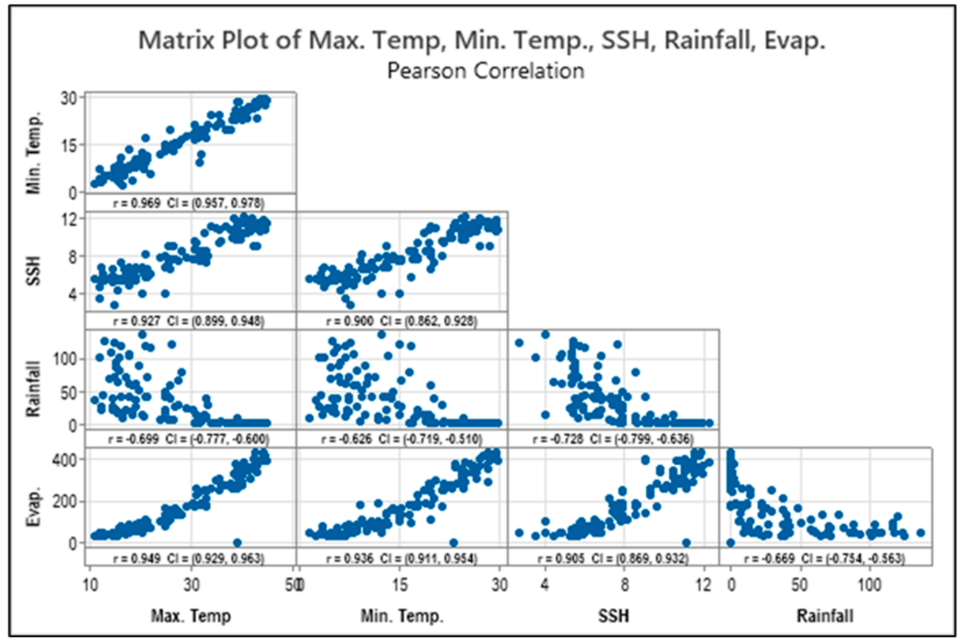
The input parameters used in this study are rainfall, minimum and maximum temperatures, and solar radiation (sunshine hours), which are utilized to predict evaporation for the same period. However, future predictions beyond 2022 and extending to 2100 are not solely based on historical data from 1980–2022. Instead, they are derived from climate projections using global and regional climate models (GCMs/RCMs) under different emission scenarios. Specifically, future climate data are generated based on Shared Socioeconomic Pathways (SSPs), including SSP2-4.5 and SSP5-8.5, which simulate future climate conditions under varying greenhouse gas emission levels.

These projected climate variables (rainfall, temperature, and solar radiation) serve as inputs into our model for estimating future evaporation rates. The model is first trained on historical data (1980–2022) to establish relationships between the input variables and evaporation. Once the model is trained, it uses the projected climate data from the SSP scenarios to predict evaporation rates for the period up to 2100.

For this study, all data were carefully calibrated, validated, and adjusted according to the specific conditions of the Kirkuk study area, following the methodology outlined in the study by [19]. The validation process involved both graphical tests (based on mean and standard deviation) and statistical tests, including the p-value and Kolmogorov–Smirnov (K-S) test, to ensure a close similarity between the measured and synthetic climate data. 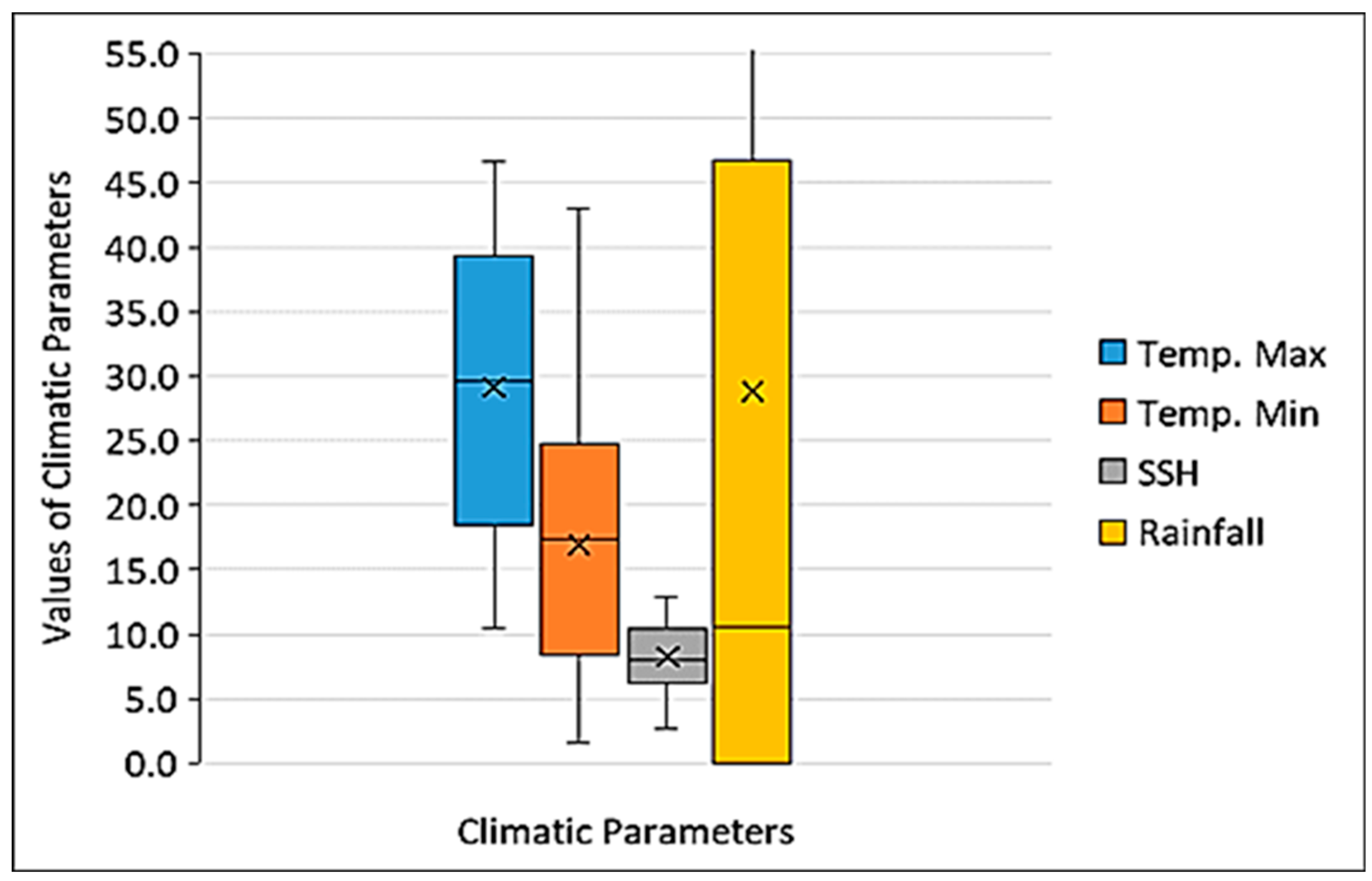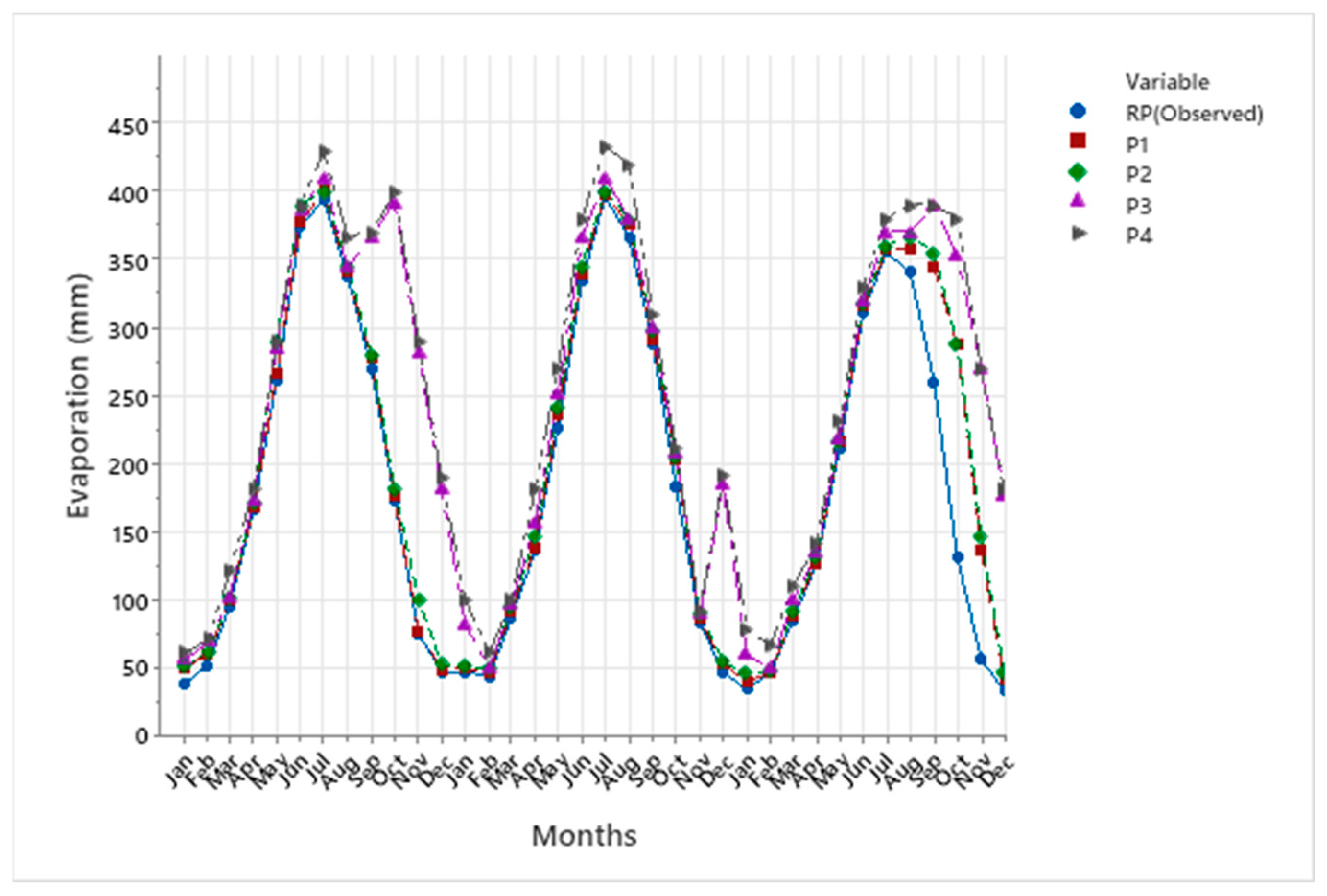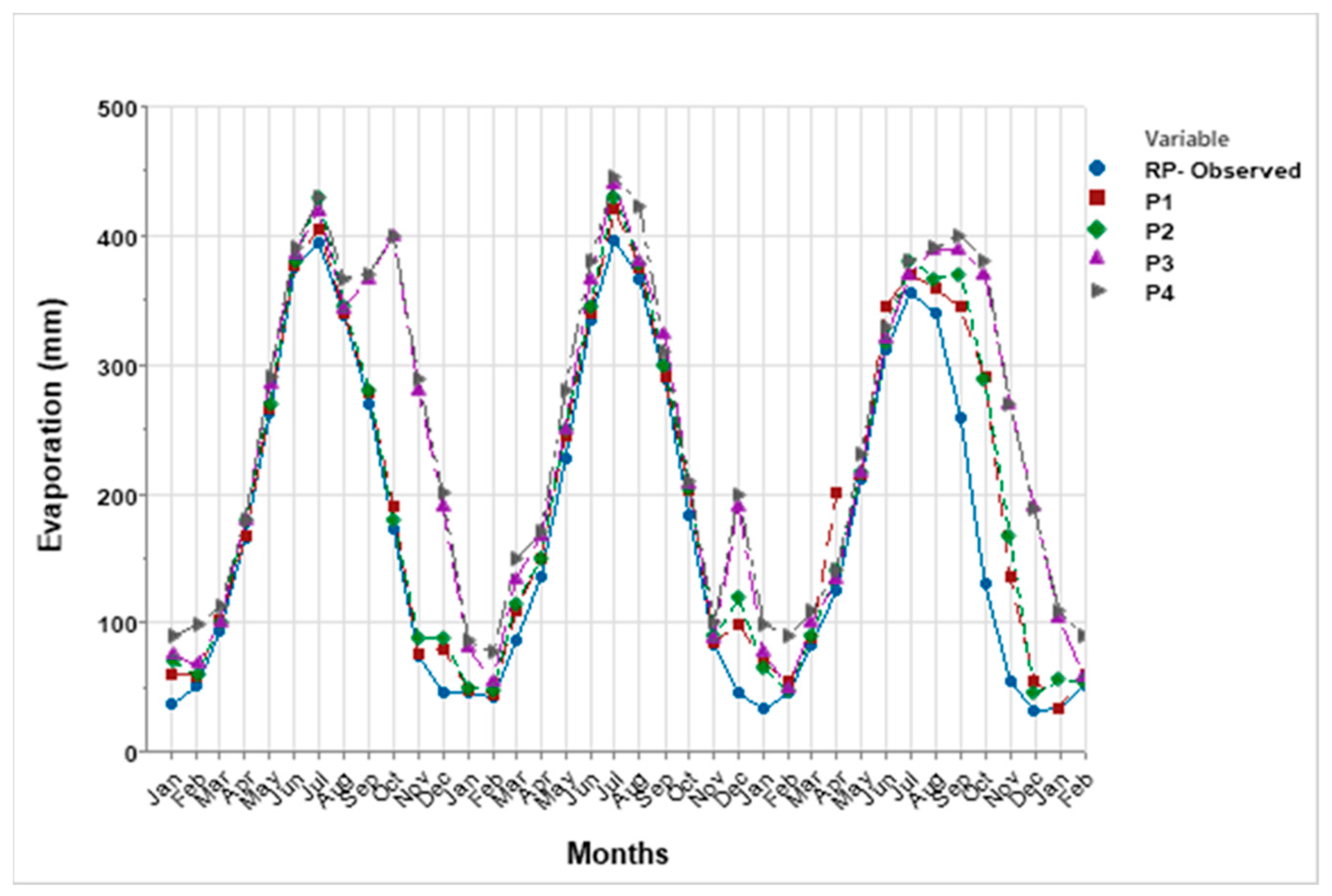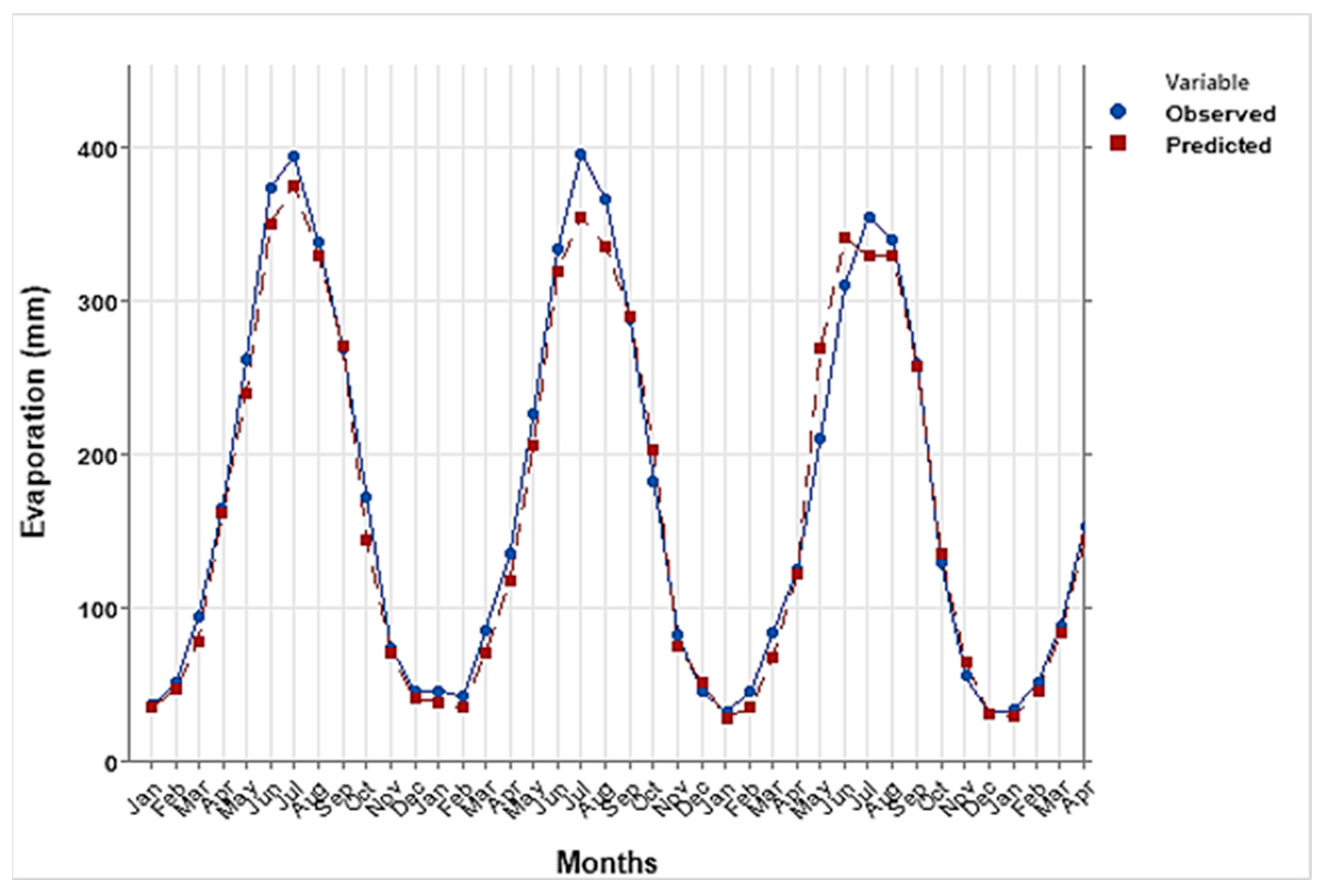Figure 3 illustrates the study’s methodological framework, providing a comprehensive overview of the steps taken in the analysis. The model uses daily input parameters, including rainfall, minimum temperature (Tmin), maximum temperature (Tmax), and sunshine hours (SSH). These daily inputs are aggregated to produce monthly evaporation estimates, which serve as the output of the model. To account for variations in the number of days per month, the model dynamically adjusts by summing or averaging daily data depending on the context. This ensures that the input dimensions remain consistent and reliable across all months, providing accurate monthly evaporation predictions. The evaporation was calculated by using Penman–Monteith evaporation method for the monthly observed evaporation.

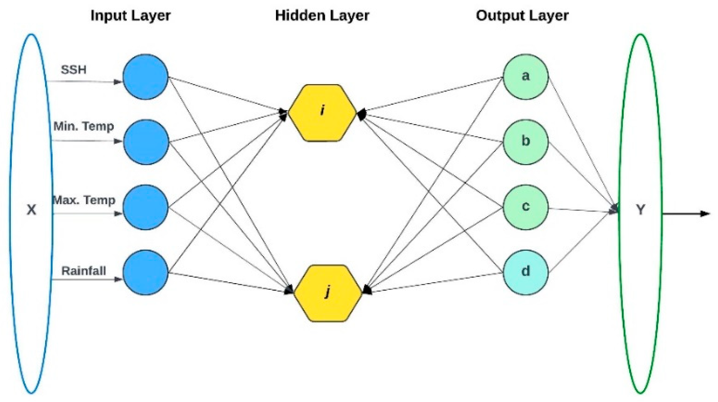
3.2. Multi-Layer Perceptron Neural Network

A multi-layer neural network, also known as a multi-layer perceptron (MLP), is an artificial neural network composed of multiple layers of interconnected nodes (neurons). Each node functions as a simple processing unit, and the network is designed to model complex relationships between inputs and outputs [8]. A multi-layer perception consists of several interconnected layers of nodes (neurons), each acting as a simple processing element. The network’s architecture is defined by the number of layers and nodes per layer [22]. These hidden layers contain neurons that serve as computational units, often described as the “black box” of the network due to their role in processing and transforming the input data through complex computations.

The architecture of an MLP is characterized by the connections between neurons, which are organized into a network of synaptic weights. Each of these weights signifies the strength of the connection between two neurons. A weight of zero indicates the absence of a connection, effectively isolating the neurons from each other.

Notably, connections between neurons are only formed between different layers; there are no intra-layer connections, meaning neurons within the same layer do not directly interact [23]. This organized structure enables the network to learn patterns and make predictions based on the input data.

Each node (neuron) in the network computes an input (I_j), which is the weighted sum of the outputs (Oj) from the nodes in the preceding layer. Mathematically, this can be expressed as:

$$I_j=i\sum Wij\times Oi$$

(1)

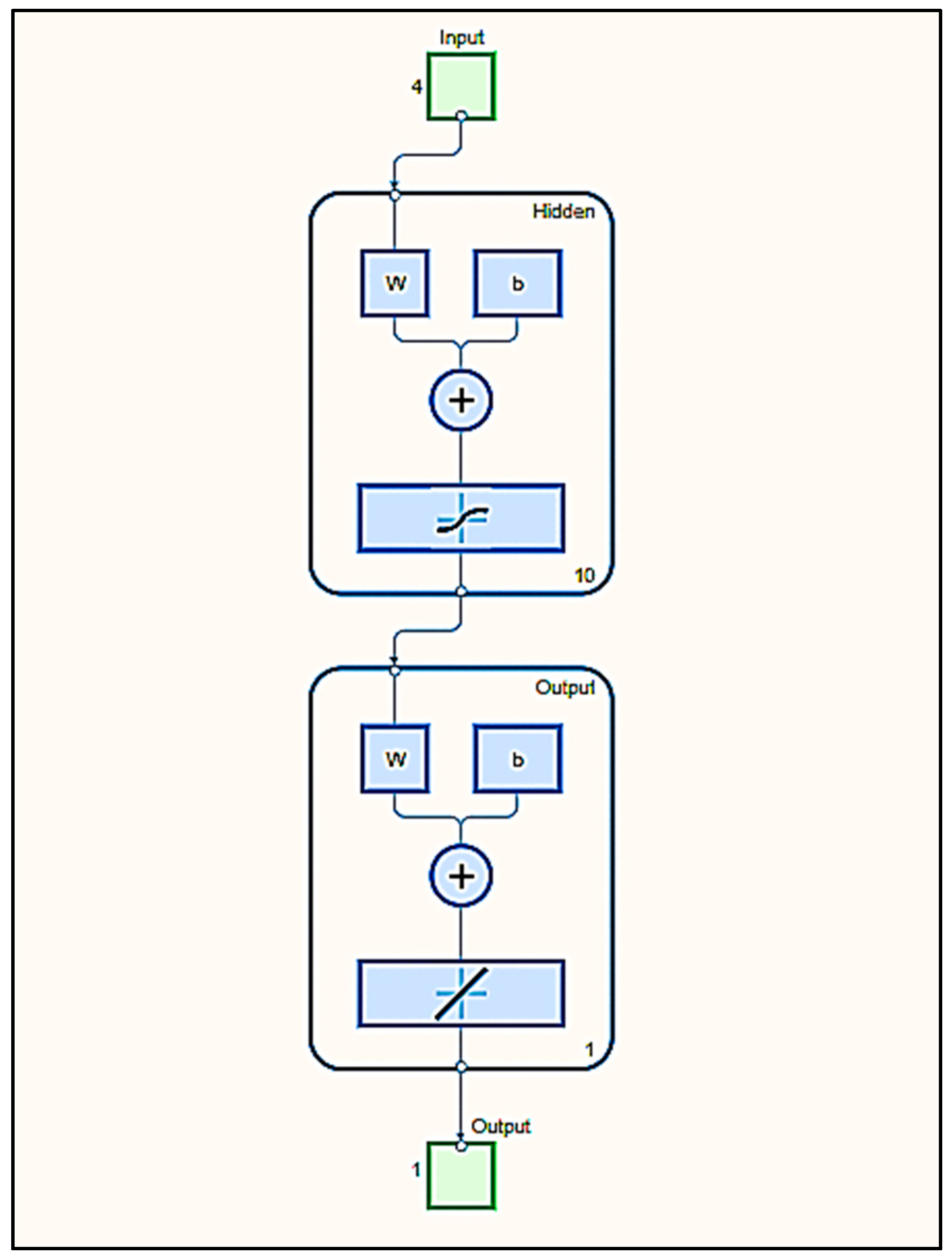
where Wij represents the weight connecting node i in the previous layer to node j in the current layer. Oi is the output of node I in the preceding layer. Figure 3 illustrates a classic MLP structure, providing a visual representation of this interconnected architecture. Figure 4 illustrates the input variables with hidden layers and output variables of MLP. Figure 5 shows the training structure of input layers and a number of variables, the hidden layers, and output layers of the multi-layer perceptron neural network of this research study.

3.3. Support Vector Machine with PCA

SVM is a powerful tool that has been extensively applied to both classification and regression tasks due to its robustness and effectiveness. SVM is not only useful for classification, but also highly effective in regression problems, where it is referred to as Support Vector Regression (SVR). The key idea behind SVM is to find a function that best fits the data while maintaining a balance between model complexity and prediction accuracy. This balance is achieved by minimizing a loss function subject to certain constraints, ensuring that the predictions are as accurate as possible while avoiding overfitting [24]. The SVM regression function can be expressed as:

$$f\left(x\right)=w.ø\left(x\right)+b$$

(2)

where w is the weight vector that defines the orientation of the hyperplane in the transformed feature space and ϕ(x) is a non-linear function that maps the input vector x into a higher-dimensional space, allowing the model to handle non-linear relationships in the data, while b is the bias term that adjusts the output to align with the target values. The objective of SVM in regression is to find the optimal weight vector w and bias b that minimize the prediction error while satisfying the margin constraints. The model tries to fit the best possible hyperplane (or line, in the case of linear regression) that lies within a predefined margin of tolerance for error. The model was combined with PCA to improve the results and minimize the error. This model was developed by using MATLAB software version 23.

3.4. Guassian Process Regression (GPR) and PCA

Gaussian Process Regression (GPR) is a non-parametric, Bayesian approach to regression that provides a probabilistic framework for modeling and predicting complex, non-linear relationships between input variables and outputs. Unlike traditional regression models, GPR offers flexibility by defining distribution over functions, allowing for the incorporation of prior knowledge and the estimation of uncertainty in predictions. The method relies on a kernel function to measure the similarity between data points, with common choices including the squared exponential and Matérn kernels [25].

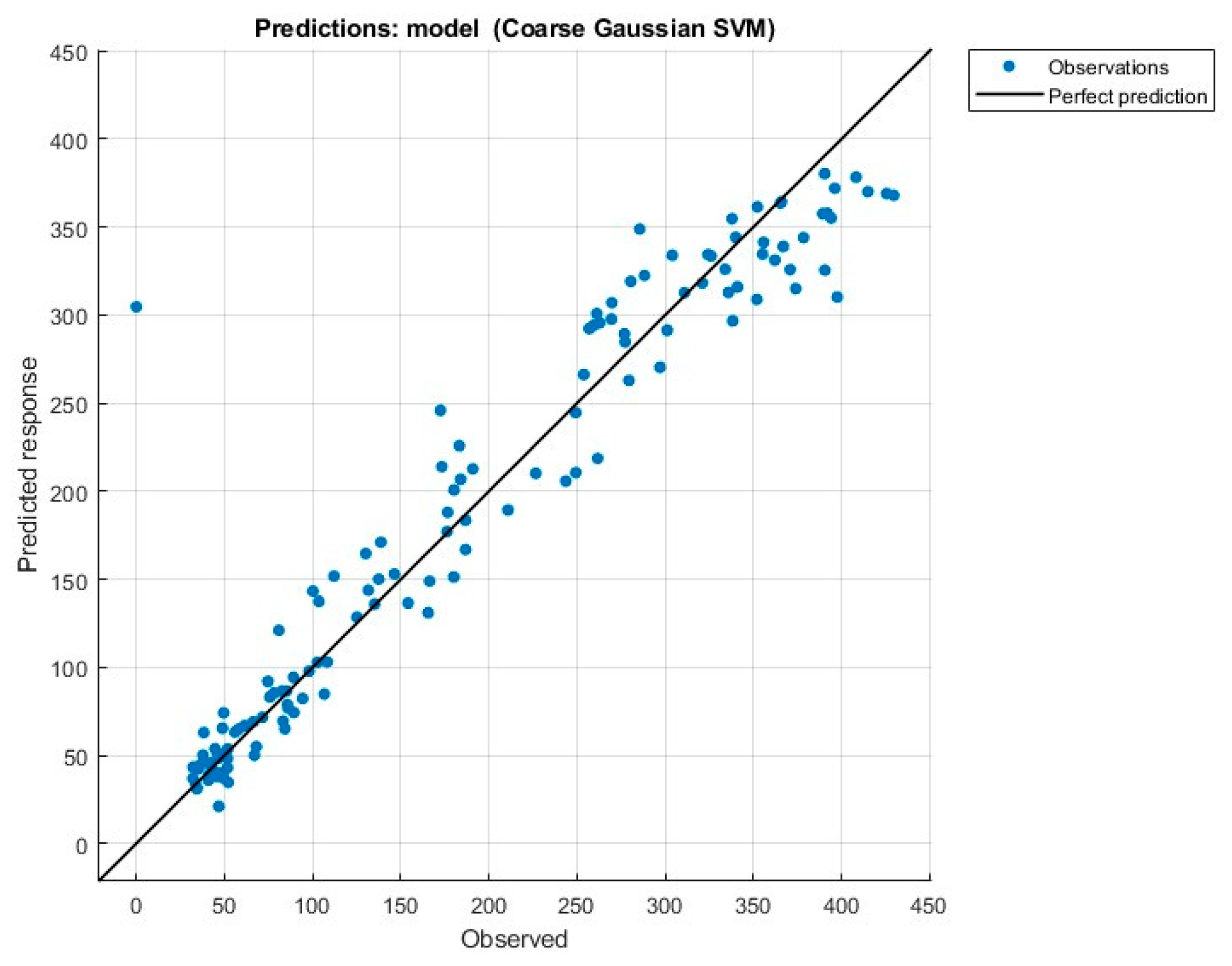
3.5. Model Evaluation and Performance

Several common statistical parameters were used to evaluate the model structures’ performance after they had been calibrated using the training dataset. According to Adamowski [24], these standards are crucial for measuring model prediction mistakes and giving a precise indication of accuracy in subsequent forecasts [25]. Several different statistical measurements, including the coefficient of correlation (R), mean absolute error (MAE), mean squared error (MSE), and root mean squared error (RMSE), will be used in the model calibration. Equations (3)–(6) provide a summary of these indications.

$$MAE={\displaystyle \frac{{\sum }_{m=1}^N\left|x_o-x_p\right|}{N}}$$

(3)

$$MSE={\displaystyle \frac{{\sum }_{m=1}^N{\left(x_o-x_p\right)}^2}{N}}$$

(4)

$$RMSE=\sqrt{{\displaystyle \frac{{\sum }_{m=1}^N{\left(x_o-x_p\right)}^2}{N}}}$$

(5)

$$R=\left[{\displaystyle \frac{{\sum }_{m=1}^N\left(x_o-\overline{x_o}\right)\left(x_p-\overline{x_p}\right)}{\sqrt{\sum {\left(x_o-\overline{x_o}\right)}^2\sum {\left(x_p-\overline{x_p}\right)}^2}}}\right]$$

(6)

where N is the sample size, x_o stands for observed water consumption, x_p for expected water demand, $\overline{x_p}$ for the mean of predicted demand, and $\overline{x_o}$ for the mean of observed consumption.

To estimate future evaporation, the projected climate data from the downscaled model are applied to an MLP. It is assumed that the model parameters, such as weights and the number of MLP neurons, remain constant in the future.

4. Results and Discussion

4.1. Evaporation Using MLP Model with PCA

To build and train the neural network for evaporation prediction, the MLP model was created using MATLAB 2023a. Numerous statistical procedures were used to evaluate the model’s functionality. The ANN model was constructed using evaporation data as its output and the daily rainfall, minimum and maximum temperature, and sunshine hour data as the input parameters. Three subsets of the dataset were created: a training set (70%), an evaluation set (15%), and a validation set (15%). The 1980–2022 timeframe for the data allowed for a rapid and effective model training approach. The data were analyzed first by applying PCA, which can help reduce overfitting and reduces dimensionality. Figure 6 illustrates the PCA analysis for the input and output climatic parameters.

The network was trained using the training set, and its performance was tracked during the training phase using the validation set. When the validation set’s error dropped to its lowest value, training was stopped. A test dataset that was not used during the training phase was then used to evaluate the model’s performance. With an R² value of 0.95, which indicates a high level of accuracy in the model’s predictions, Figure 7 shows the relationship and validation model between the observed and projected evaporation. The time series and relationship between the simulated and observed evaporation for the historical data (1980–2022) are displayed in Figure 8. The model performed well, as the observed and simulated results closely aligned, showing only an R² of 0.95, which indicates a good performance and accuracy for the model.

In comparison to the baseline era, the evaporation rate for period P1 (2031–2050) increased by about 1.5% under the SSP2-4.5 scenario. There was a 1.73% increase for P2 (2051–2070) and a 1.81% increase for P3 (2071–2090). P4 (2091–2100) had the largest increase, with the evaporation rate rising by almost 2.12% above the baseline. With rises of 1.76% and 1.87% in P1 and P2, respectively, and 1.92% and 2.23% in P3 and P4, the SSP5-8.5 scenario demonstrated higher evaporation increases than SSP2-4.5. In the Kirkuk study area, the SSP5-8.5 scenario had a greater effect on evaporation than SSP2-4.5. Figure 9 and Figure 10, respectively, display time series data for evaporation over all time periods under the SSP2-4.5 and SSP5-8.5 scenarios for MLP with PCA.

Table 2. Evaluation of Three Average Evaporation Models.

Model Input Type	MAE (mm)	RMSE (mm)	R2
MLP	0.02	0.10	0.95
SVM	0.21	0.13	0.92
GPR	0.22	0.37	0.91

presents the evaluation results for the MSE, MAE, and R² of the three average evaporation models.

4.2. Evaporation Using SVM Model with PCA

The second model was developed using Support Vector Machine (SVM) techniques to predict and estimate evaporation. An SVM is a non-statistical binary classification technique that has gained significant attention from researchers in recent years [26]. There are two types of SVM models: Support Vector Classification (SVC) and Support Vector Regression (SVR). While SVC is used for classifying data into different categories, the SVR framework is designed for prediction problems [27] This study applied the SVR model using four predictors: rainfall, minimum temperature (minT), maximum temperature (maxT), and sunshine hours (SSH). Figure 11 illustrates the validation model for the mean ensemble evaporation with an R² value of 0.92, indicating good model accuracy, although it is slightly lower than the Neural Network model. Figure 12 shows the relationship between the observed and predicted evaporation values in the time series for SVM with PCA. Under the SSP2-4.5 scenario, the evaporation rate for period P1 (2031–2050) showed a slight increase of 1.61%, while for periods P2 (2051–2070) and P3 (2071–2090), the increases were smaller, at 1.89% and 1.93%, respectively. The highest increase occurred in P4 (2091–2100), with a rate of 2.68%, compared to an observed value increase of 1.33%. Figure 13 and Figure 14 depict the evaporation time series under both the SSP2-4.5 and SSP5-8.5 scenarios for SVM with PCA.

4.3. Evaporation Gaussian Process Regression (GPR with PCA)

Figure 15 illustrates the validation model of observed values versus the predicted values for evaporation. The R² value equals 0.91. Figure 16 demonstrates the time series values for observed and predicted values for the historical data (1980–2022). While Figure 17 depicts the time series of observed and predicted evaporation values for all periods under the SSP2-4.5 scenario. The evaporation values increased under the SSP5-8.5 scenarios and as illustrated in Figure 18.

The future projection for evaporation is increased for both models MLP and SVM but the MAE, and RMSE for the MLP model are less than in SVM for all periods and under both climate scenarios. The ensemble validation R² for MLP is 0.95 and higher than in SVM which is 0.92, the MAE RMSE for MLP model values were 0.02 mm and 0.10 mm respectively, and less than the validation values of SVM of 0.21 mm, and 0.13 mm which means that MLP model is more accurate and reliable than SVM model. While GPR model showed values of model performance for MAE, and RMSE equal to 0.22 mm and 0.37 mm respectively. Therefore, the performance of the MLP technique is more adequate than the SVM and GPR models. The following

Table 3. The average annual evaporation of RP/historical compared to future projection evaporation under the SSP2-4.5 and SSP5-8.5 scenarios.

Scenario	AV. Evaporation mm year−1				Av. Evaporation Rate Change %
Baseline period	1370.9				-
SSP2-4.5	P1	P2	P3	P4	57.2%
	1634.1	1651.3	1671.8	1689.8
SSP5-8.5	1732.2	1744.2	1753.4	1764.3	85.9%

shows the average annual evaporation of the baseline compared to future projection evaporation under the SSP2-4.5 and SSP5-8.5 scenarios.

4.4. Evaporation Using SVM, MLP, and GPR with PCA

Compared to the baseline period, the evaporation rate under the SSP2-4.5 scenario shows a gradual increase across future periods. The percentage increases in evaporation rates presented in this research are based on the comparison between baseline historical evaporation rates (1980–2022) and the future predicted rates under the SSP2-4.5 and SSP5-8.5 climate scenarios. For P1 (2031–2050), evaporation rises by approximately 1.5%. This increase continues with a 1.73% rise in P2 (2051–2070) and 1.81% in P3 (2071–2090). The largest increase occurs in P4 (2091–2100), where the rate climbs by nearly 2.12% above the baseline. In contrast, the SSP5-8.5 scenario presents higher increases in evaporation across all periods compared to SSP2-4.5. For P1 and P2, the evaporation rate increases by 1.76% and 1.87%, respectively. In P3, it rises by 1.92%, while in P4, the increase reaches 2.23%. These figures demonstrate that the SSP5-8.5 scenario has a stronger impact on evaporation, particularly in the Kirkuk study area, where its effect is more pronounced than under SSP2-4.5. The MAE and RMSE values for MLP were 0.02 and 0.10, respectively; compared to the SVM values with PCA, the values were higher and equal to 0.21 and 0.13, respectively, and for the evaporation rates under the SSP2-4.5 scenario, the evaporation rate for period P1 (2031–2050) showed a slight increase of 1.61%, while for periods P2 (2051–2070) and P3 (2071–2090), the increases were smaller, at 1.89% and 1.93%, respectively. The highest increase occurred in P4 (2091–2100), with a rate of 2.68%, compared to an observed value increase of 1.33%. For GPR with PCA values of the model performance for MAE and RMSE, the results were equal to 0.22 and 0.37, respectively, and higher than the MLP and SVM with PCA. Therefore, the performance of the MLP technique is more adequate than the SVM and GPR models with PCA. The average annual evaporation was calculated by using the Penman–Monteith method as a baseline period and as following in Table 3.

The average evaporation rate change under SSP2-4.5 was 57.2 and 85.9%while under SSP5-8.5 respectively, which means that the evaporation rate is increased under the SSP5-8.5 scenario compared to baseline period and SSP2-4.5 scenario and that The MLP model has been approved and validated as the best model for evaporation prediction for this study.

5. Conclusions

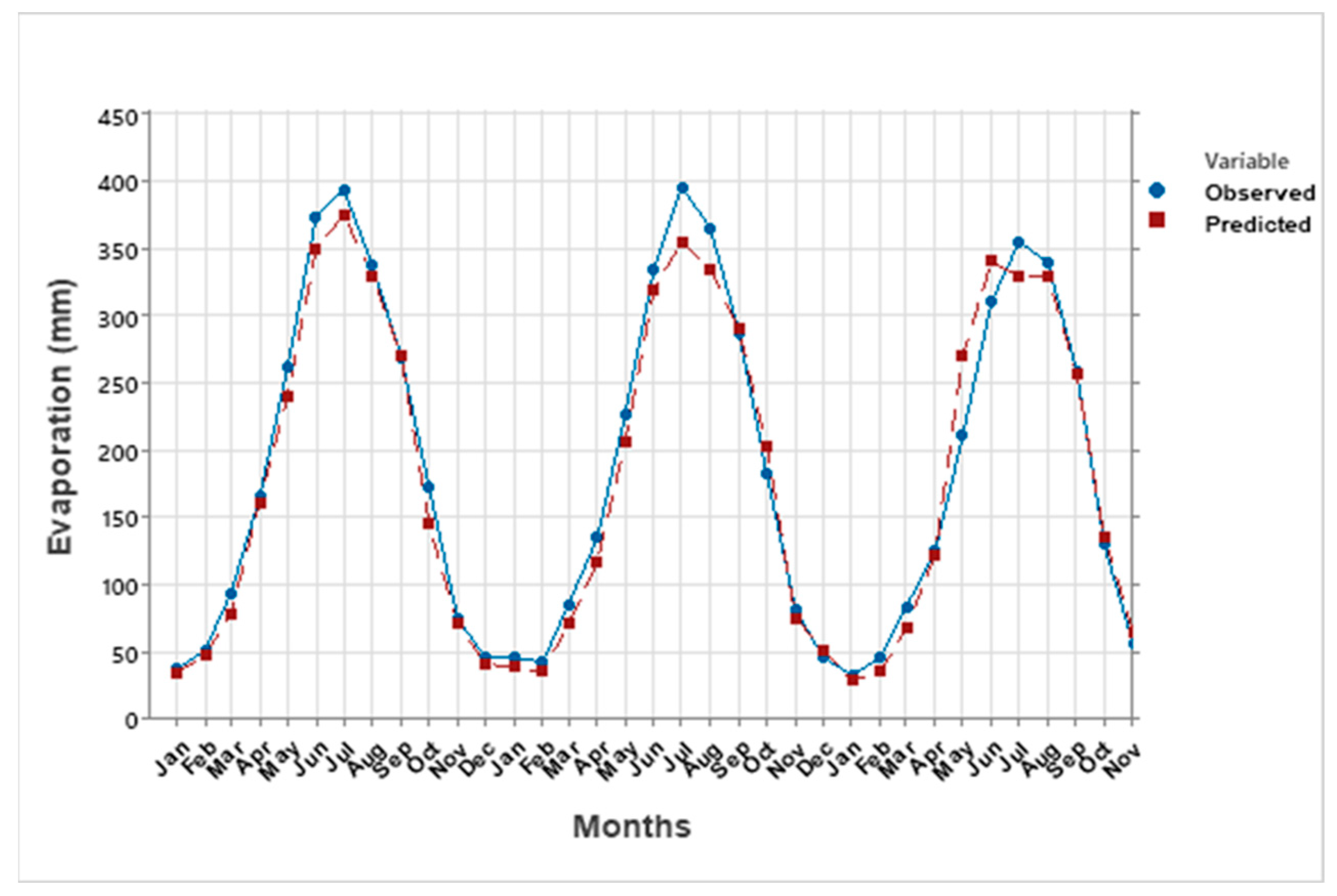
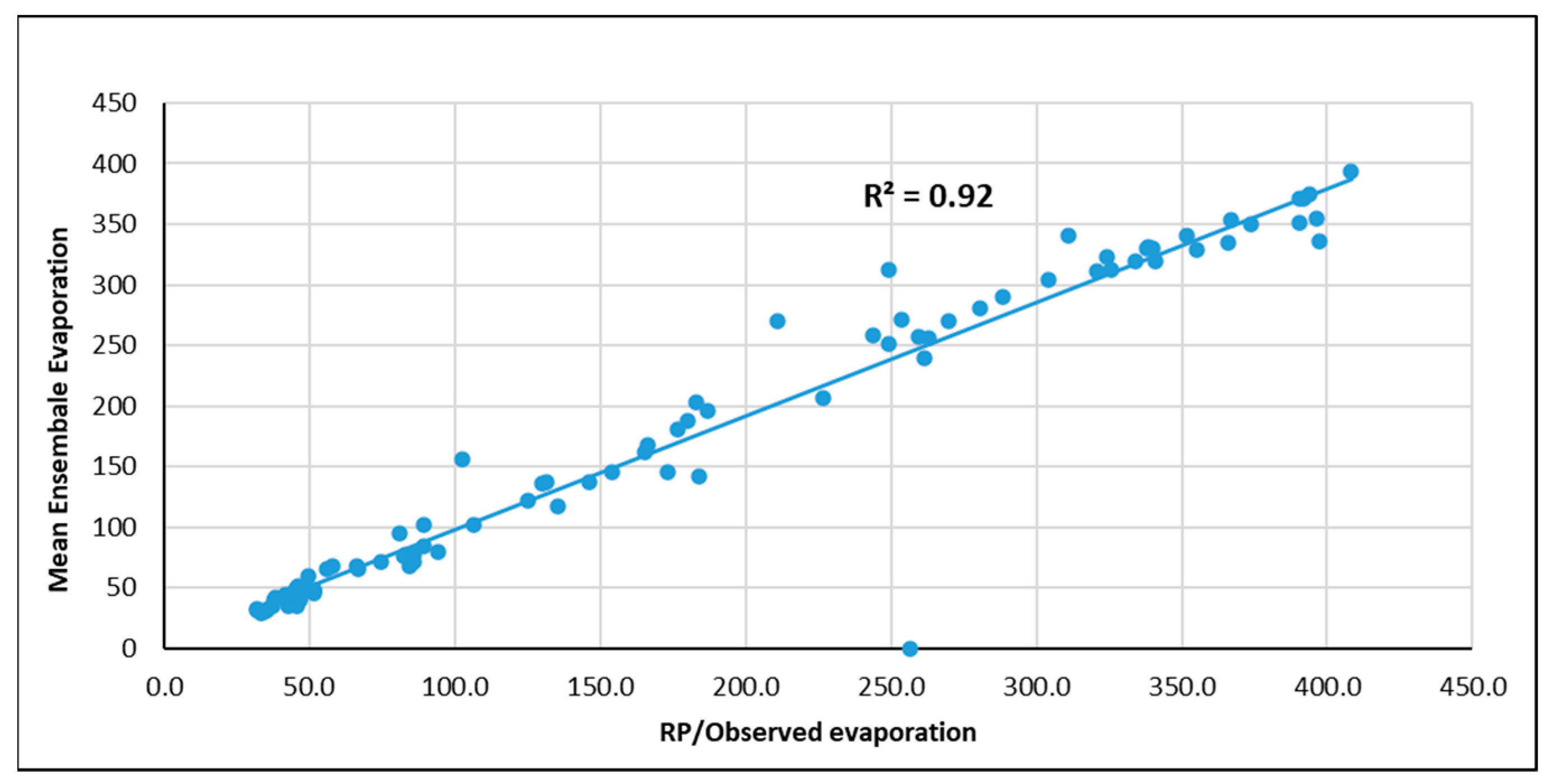
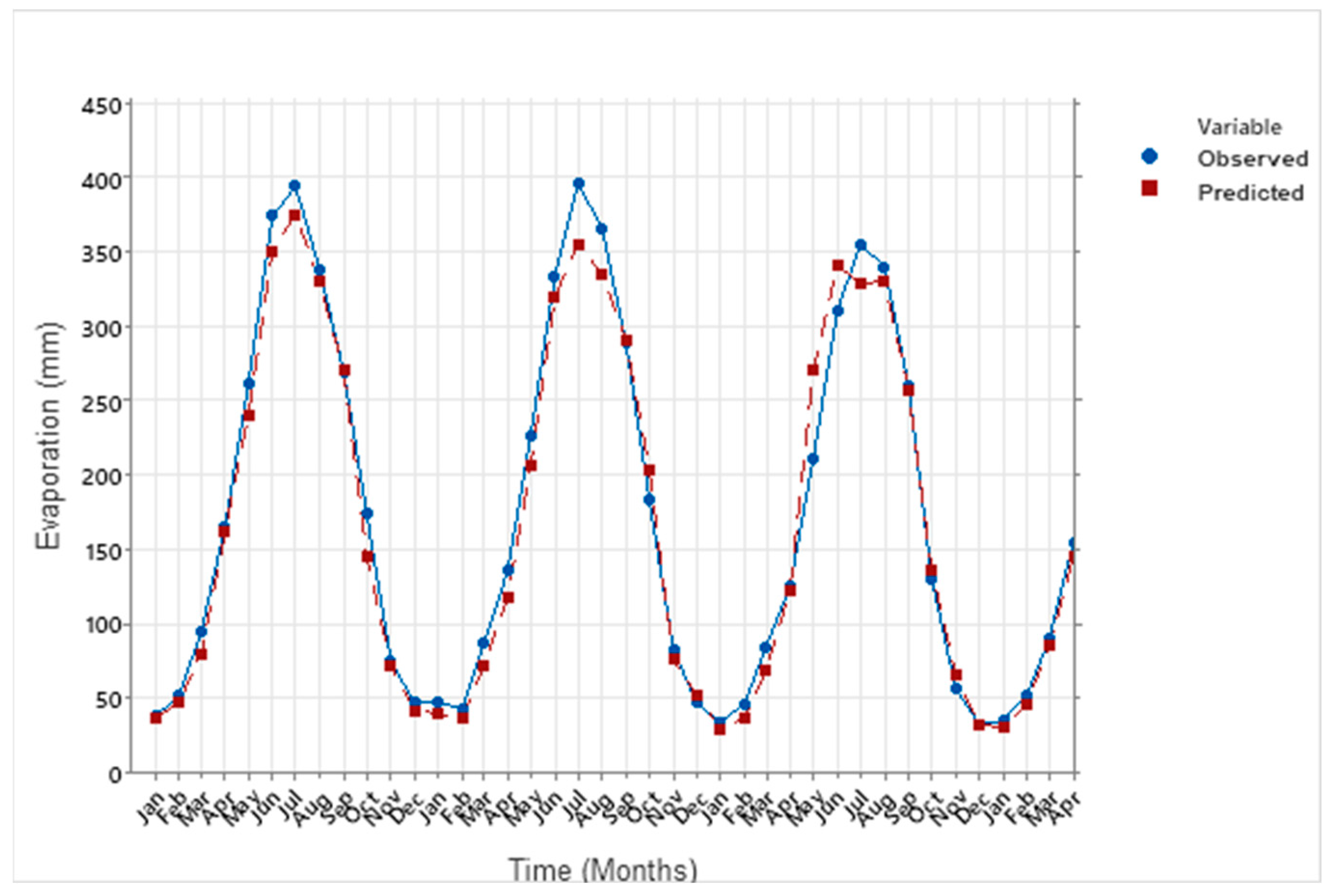
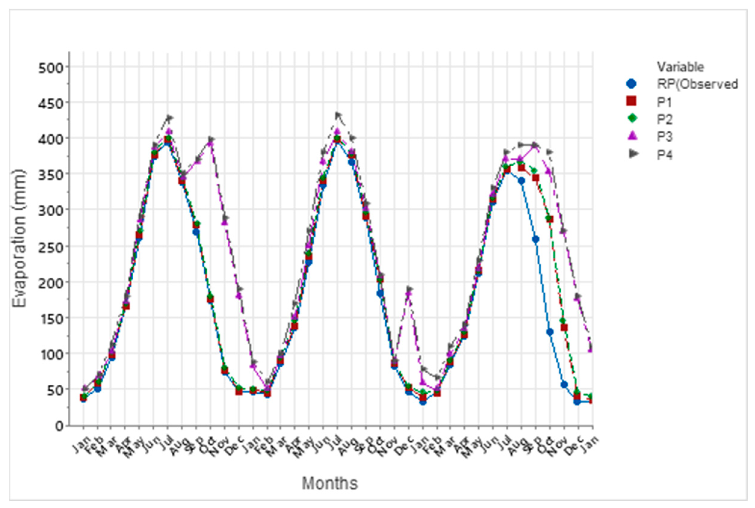
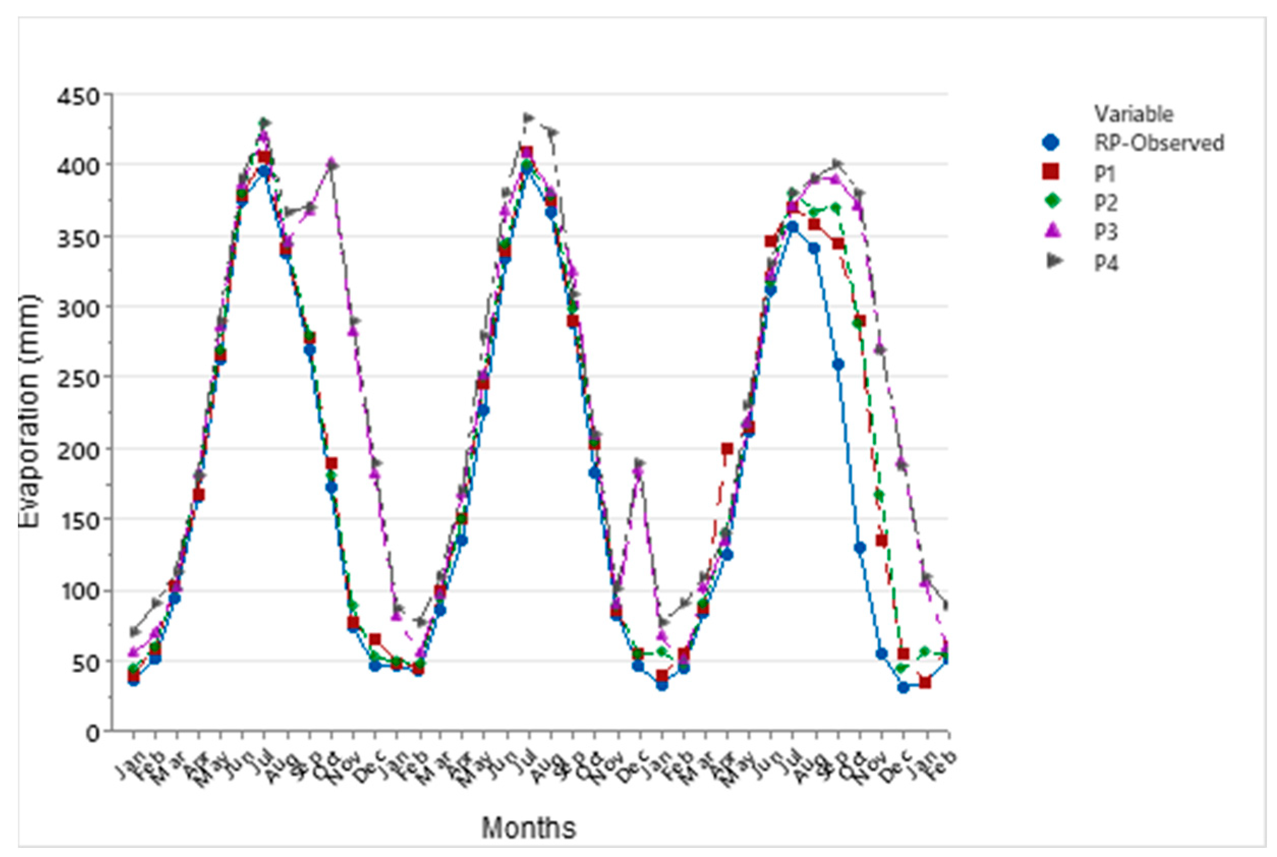
Evaporation plays a critical role in the hydrological cycle, though its natural process is inherently complex and often unpredictable. In this study, we utilized machine learning techniques, namely the Multi-Layer Perceptron (MLP), Support Vector Machine (SVM), and Gaussian Process Regression (GPR) with Principal Component Analysis (PCA), to estimate and predict evaporation rates. These models were based on historical data and future projections under two climate scenarios: SSP2-4.5 and SSP5-8.5. Among these techniques, the MLP model demonstrated a superior performance, providing the most accurate evaporation estimates compared to the SVM and GPR models, though all three were effective.

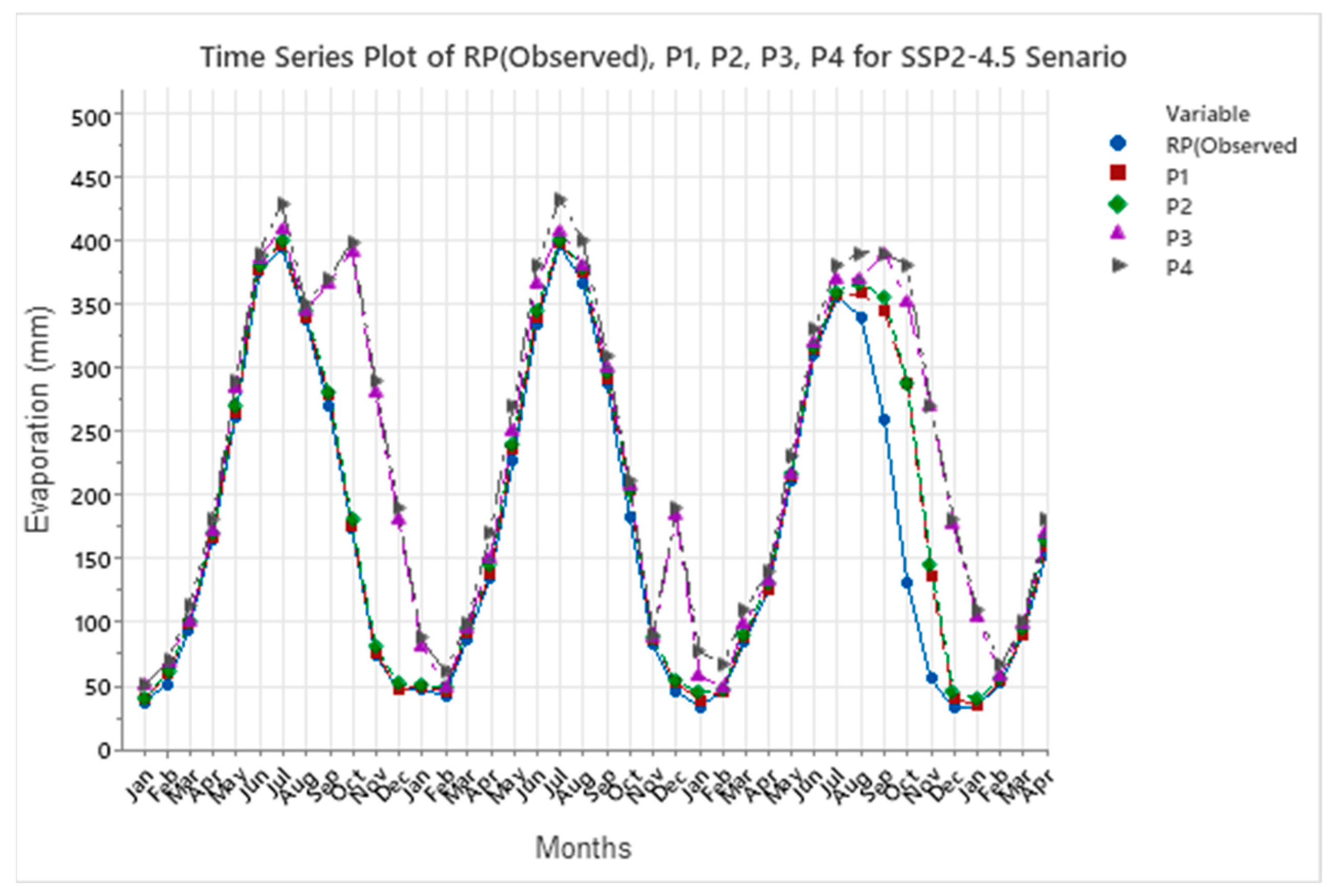
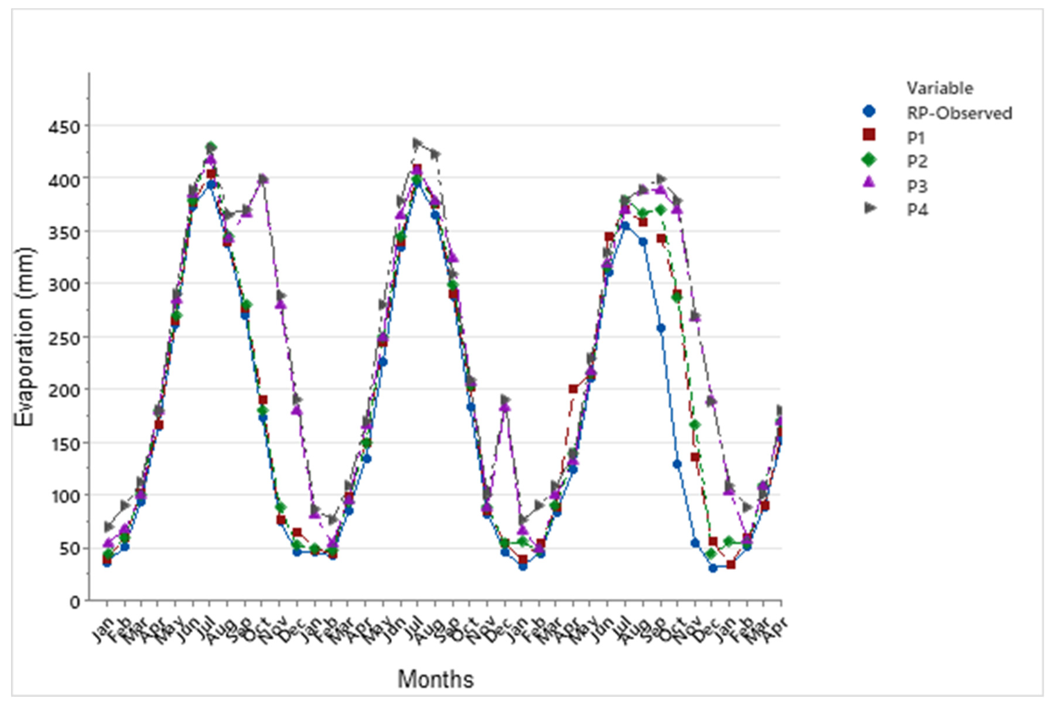
The evaporation model incorporated key input variables such as rainfall, sunshine hours (SSH), and the minimum and maximum temperatures (Tmin and Tmax). Both the SSP2-4.5 and SSP5-8.5 climate scenarios indicated an increase in evaporation rates, with SSP5-8.5 exhibiting a notably larger rise. When compared to historical evaporation rates, the SSP5-8.5 scenario projected a significantly greater increase than SSP2-4.5, highlighting the impact of more extreme climate changes.

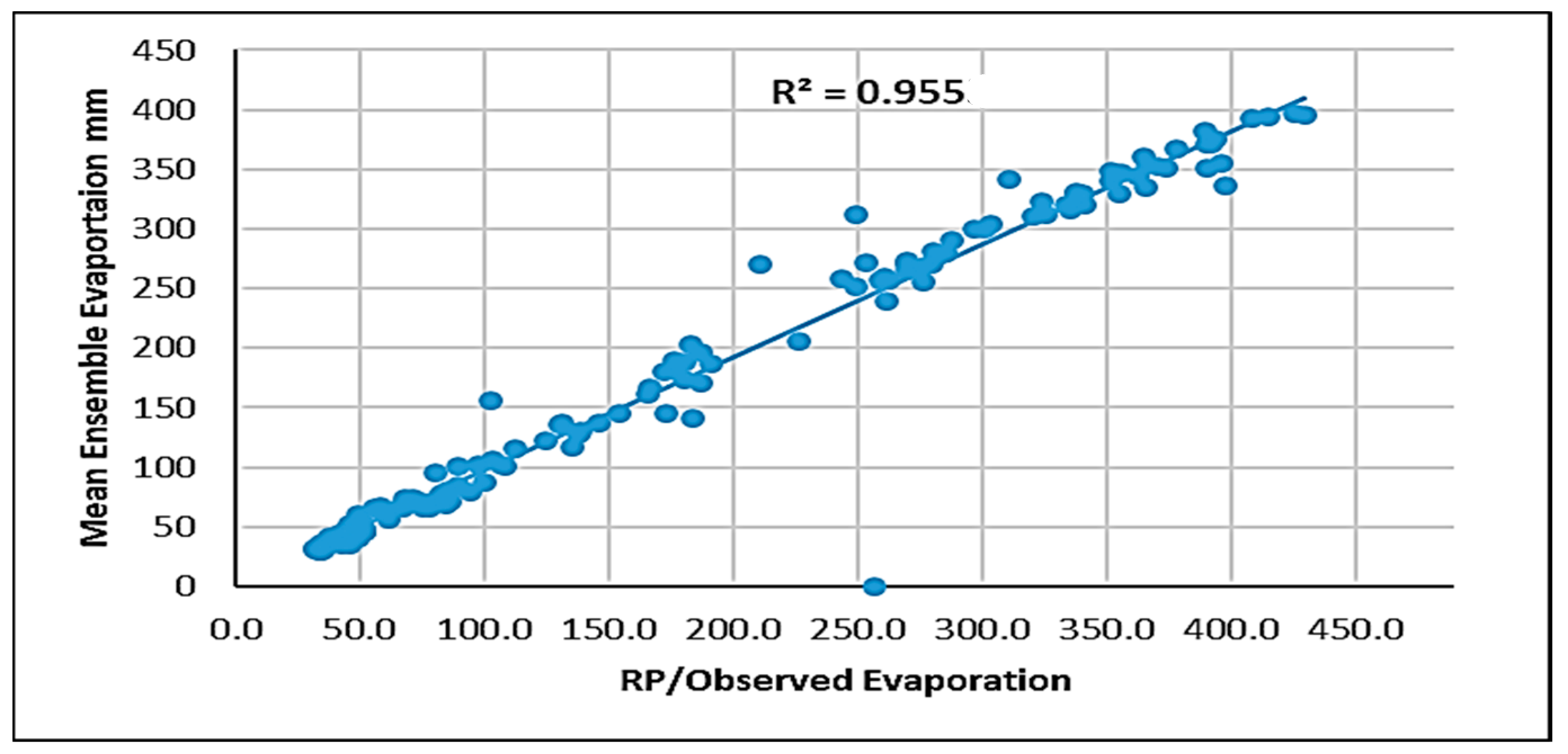
The evaluation values for GPR with PCA, MAE and RMSE are equal to 0.22 and 0.37 mm respectively, and higher than SVM with PCA and MLP equal to (0.21, 0.13, 0.02, and 0.10 mm respectively). This study underscores the importance of estimating and forecasting evaporation rates, particularly in the context of changing climates, which is especially relevant for semi-arid regions where the impacts on water resources are more pronounced. The findings emphasize the need for resilient and sustainable water management strategies to ensure future water security in these vulnerable areas.

References

1. Konapala, G.; Mishra, A.K.; Wada, Y.; Mann, M.E. Climate change will affect global water availability through compounding changes in seasonal precipitation and evaporation. Nat. Commun. 2020, 11, 3044. [Google Scholar] [PubMed]
2. Gianotti, D.J.S.; Akbar, R.; Feldman, A.F.; Salvucci, G.D.; Entekhabi, D. Terrestrial Evaporation and Moisture Drainage in a Warmer Climate. Geophys. Res. Lett. 2020, 47, e2019GL086498. [Google Scholar]
3. Ghaemi, A.; Rezaie-Balf, M.; Adamowski, J.; Kisi, O.; Quilty, J. On the applicability of maximum overlap discrete wavelet transform integrated with MARS and M5 model tree for monthly pan evaporation prediction. Agric. For. Meteorol. 2019, 278, 107647. [Google Scholar]
4. Jing, W.; Yaseen, Z.M.; Shahid, S.; Saggi, M.K.; Tao, H.; Kisi, O.; Salih, S.Q.; Al-Ansari, N.; Chau, K.-W. Implementation of evolutionary computing models for reference evapotranspiration modeling: Short review, assessment and possible future research directions. Eng. Appl. Comput. Fluid Mech. 2019, 13, 811–823. [Google Scholar]
5. Kapli, F.W.A.; Azis, F.A.; Suhaimi, H.; Shamsuddin, N.; Abas, P.E. Feasibility Studies of Rainwater Harvesting System for Ablution Purposes. Water 2023, 15, 1686. [Google Scholar] [CrossRef]
6. Fan, J.; Wu, H.; Wang, F. Evaporation-driven liquid flow through nanochannels. Phys. Fluids 2020, 32, 012001. [Google Scholar]
7. Al Sudani, Z.A.; Salem, G.S.A. Evaporation Rate Prediction Using Advanced Machine Learning Models: A Comparative Study. Adv. Meteorol. 2022, 2022, 1433835. [Google Scholar]
8. Ghorbani, M.A.; Deo, R.C.; Yaseen, Z.M.; Kashani, M.H.; Mohammadi, B. Pan evaporation prediction using a hybrid multilayer perceptron-firefly algorithm (MLP-FFA) model: Case study in North Iran. Theor. Appl. Clim. 2018, 133, 1119–1131. [Google Scholar]
9. Moghaddamnia, A.; Gousheh, M.G.; Piri, J.; Amin, S.; Han, D. Evaporation estimation using artificial neural networks and adaptive neuro-fuzzy inference system techniques. Adv. Water Resour. 2009, 32, 88–97. [Google Scholar]
10. Fahimi, F.; Yaseen, Z.M.; El-Shafie, A. Application of soft computing based hybrid models in hydrological variables modeling: A comprehensive review. Theor. Appl. Clim. 2017, 128, 875–903. [Google Scholar]
11. Gocić, M.; Motamedi, S.; Shamshirband, S.; Petković, D.; Ch, S.; Hashim, R.; Arif, M. Soft computing approaches for forecasting reference evapotranspiration. Comput. Electron. Agric. 2015, 113, 164–173. [Google Scholar]
12. Ghorbani, M.A.; Shamshirband, S.; Haghi, D.Z.; Azani, A.; Bonakdari, H.; Ebtehaj, I. Application of firefly algorithm-based support vector machines for prediction of field capacity and permanent wilting point. Soil Tillage Res. 2017, 172, 32–38. [Google Scholar]
13. Hamza, Z.A.H. Predicted evaporation in Basrah using artificial neural networks. Open Eng. 2024, 14, 20220590. [Google Scholar]
14. Rai, P.; Kumar, P.; Al-Ansari, N.; Malik, A. Evaluation of Machine Learning versus Empirical Models for Monthly Reference Evapotranspiration Estimation in Uttar Pradesh and Uttarakhand States, India. Sustainability 2022, 14, 5771. [Google Scholar] [CrossRef]
15. Abdulrahman, S.A. The drying up of the Lower Zab River and future water disputes between Iran, Kurdistan Region and Iraq. Int. J. Environ. Stud. 2018, 75, 29–44. [Google Scholar]
16. Daniels, A.E.; Morrison, J.F.; Joyce, L.A.; Crookston, N.L.; Chen, S.C.; McNulty, S.G. Climate Projections FAQ; General Technical Report RMRS-GTR-277WWW; US Department of Agriculture, Forest Service, Rocky Mountain Research Station: Fort Collins, CO, USA, 2012; 32p.
17. Trzaska, S.; Schnarr, E. A review of downscaling methods for climate change projections. United States Agency Int. Dev. By Tetra Tech. ARD 2014, 2014, 1–42. [Google Scholar]
18. Al-Hasani, B.; Abdellatif, M.; Carnacina, I.; Harris, C.; Al-Quraishi, A.; Maaroof, B.F.; Zubaidi, S.L. Integrated geospatial approach for adaptive rainwater harvesting site selection under the impact of climate change. Stoch. Environ. Res. Risk Assess. 2024, 38, 1009–1033. [Google Scholar]
19. Semenov, M.A.; Pilkington-Bennett, S.; Calanca, P. Validation of ELPIS 1980-2010 baseline scenarios using the observed European Climate Assessment data set. Clim. Res. 2013, 57, 1–9. [Google Scholar]
20. Semenov, M.A. Simulation of extreme weather events by a stochastic weather generator. Clim. Res. 2008, 35, 203–212. [Google Scholar]
21. Iraqi Meteorological Organization. Climatical Data for Kirkuk, Dakuk and Ton Kobri, Taza, Dibis Stations for Period (1980–2010); Iraqi Meteorological Organization: Baghdad, Iraq, 2017.
22. Tezel, G.; Buyukyildiz, M. Monthly evaporation forecasting using artificial neural networks and support vector machines. Theor. Appl. Clim. 2016, 124, 69–80. [Google Scholar]
23. Sayadi, A.; Monjezi, M.; Talebi, N.; Khandelwal, M. A comparative study on the application of various artificial neural networks to simultaneous prediction of rock fragmentation and backbreak. J. Rock Mech. Geotech. Eng. 2013, 5, 318–324. [Google Scholar]
24. Sadia, M. Application of Machine Learning in Analyzing Severities of Double Vehicle Crashes in Bangladesh. Master’s Thesis, Bangladesh University of Engineering and Technology (BUET), Dhaka, Bangladesh, 2023. [Google Scholar]
25. Williams, C.K.; Rasmussen, C.E. Gaussian Processes for Machine Learning; MIT Press: Cambridge, MA, USA, 2006; Volume 2, p. 4. [Google Scholar]
26. Naganna, S.R.; Deka, P.C.; Ghorbani, M.A.; Biazar, S.M.; Al-Ansari, N.; Yaseen, Z.M. Dew point temperature estimation: Application of artificial intelligence model integrated with nature-inspired optimization algorithms. Water 2019, 11, 742. [Google Scholar] [CrossRef]
27. Abed, M.; Imteaz, M.; Ahmed, A.N.; Huang, Y.F. Improved prediction of monthly pan evaporation utilising support vector machine technique. In Proceedings of the 2021 IEEE Asia-Pacific Conference on Computer Science and Data Engineering (CSDE), Brisbane, Australia, 8–10 December 2021; pp. 1–5. [Google Scholar]
Figure 1. Climatic parameters.
Water 17 01039 g001
Figure 2. Correlation test.
Water 17 01039 g002
Figure 3. Methodology flow-chart diagram.
Water 17 01039 g003
Figure 4. Structure of MLP.
Water 17 01039 g004
Figure 5. The training structure of MLP.
Water 17 01039 g005
Figure 6. PCA analysis for climatic data.
Water 17 01039 g006
Figure 7. Validation model for observed and predicted evaporation for MLP.
Water 17 01039 g007
Figure 8. Time series of observed and predicted evaporation for MLP and PCA.
Water 17 01039 g008
Figure 9. Time series evaporation under SSP2-4.5 scenario for MLP and PCA.
Water 17 01039 g009
Figure 10. Time series evaporation under SSP5-8.5 scenario for MLP and PCA.
Water 17 01039 g010
Figure 11. Validation model for observed and predicted evaporation for SVM with PCA.
Water 17 01039 g011
Figure 12. Time series of observed and predicted evaporation for SVM with PCA.
Water 17 01039 g012
Figure 13. Time series of evaporation under SSP2-4.5 scenario for SVM with PCA.
Water 17 01039 g013
Figure 14. Time series of evaporation under SSP5-8.5 scenario for SVM with PCA.
Water 17 01039 g014
Figure 15. The validation model of observed versus the predicted evaporation.
Water 17 01039 g015
Figure 16. The time series of observed and predicted evaporation.
Water 17 01039 g016
Figure 17. Time series of evaporation under SSP2-4.5 scenario.
Water 17 01039 g017
Figure 18. Time series of evaporation under SSP5-8.5 scenario.
Water 17 01039 g018