Mixing Regimes in a Shallow Lake over the Past Five Decades: Application to Laguna Carén

Abstract

This study presents a 50-year hydrodynamic simulation of Laguna Carén, a shallow lake near the capital of Chile, utilizing the 3-Dimensional coupled Hydrodynamic-Aquatic Ecosystem Model, AEM3D, to investigate the factors influencing the mixing regimes of the water column. The model incorporates key processes, such as heat and momentum exchanges with the atmosphere, light penetration, and heat diffusion in sediments, all fundamental for understanding the hydrodynamics of the lake. The obtained results allowed classifying the mixing regime of the lake in rarely mixed (RM), intermittently mixed (IM), and often-mixed (RM) regimes. Furthermore, the numerical results reveal a significant differentiation between IM and OM years, primarily driven by changes in meteorological forces, particularly wind speed. The analysis indicates that increased wind speeds enhance turbulent kinetic energy, leading to a reduction in the percentage of time the water column is stratified, whereas lower wind conditions promote stable stratification. This study shows that the mixing regime in shallow lakes can exhibit dramatic changes in response to minor alterations in meteorological conditions, particularly wind speed. Such changes in mixing regimes may result in unpredictable consequences for the ecology of the lake.

1. Introduction

Shallow lakes and wetlands are vital hotspots of biodiversity and play an active role in the carbon biochemical cycle within their catchments [1,2]. A crucial first step toward their conservation and management is to study how they depend on and interact with their surrounding natural and human-made environments. This understanding is essential for achieving global development goals related to climate change mitigation and nature restoration [3]. To comprehend the behavior and interactions of shallow lakes and wetlands with their environment, it is important to recognize that they are neither stratified lakes nor deep, well-mixed rivers. Understanding the transport and mixing regimes within these water bodies is necessary. Holgerson et al. [4] identified three categories of mixing regimes in shallow lakes—rarely, intermittently, and often mixed—based on the fraction of the day during which the vertical density gradient exceeds a specific threshold. These mixing regimes significantly influence organic matter decomposition and other biogeochemical processes, potentially leading to anoxic conditions in deeper waters [5,6]. Moreover, temporal variations in lakes have been recognized as important indicators of the impacts of climate change on both the lakes themselves and their catchments [7,8].

Turbulent diffusion is the primary vertical transport mechanism in lakes, influenced by the vertical gradient of water density, which can be either stable or unstable, thereby either dampening or promoting vertical transport within the system [9,10,11,12]. The resulting mixing regime of a lake can be understood as a manifestation of the ratio between the turbulent kinetic energy available for mixing and the potential energy that is required to mix the water column. Some of this external energy is dissipated through viscous friction, while the remainder is utilized to mix a stratified water column, contributing to the increase in the potential energy of the lake [13,14,15,16]. The primary sources of turbulent kinetic energy include wind shear stress and unstable conditions in the water column. In temperate lakes with water temperatures larger than 4 °C, these conditions may arise from surface cooling, which increases water density at the surface of the lake, or deep warming, which reduces water density in the deeper regions [9]. Conversely, the onset of stratification in temperate lakes may be driven by an increase in surface layer temperature due to shortwave solar radiation and other heat fluxes at the air–water interface (AWI) [11,13]. Alternatively, it can also result from the cooling of deep waters due to cold water intrusion or heat flux at the sediment–water interface (SWI) [17,18].

The exchange of heat and momentum at the AWI is well documented [19,20] and is influenced by meteorological factors that are changing due to climate change. To study the effects of climate change on the mixing regime of shallow lakes, it is essential to focus not only on increasing air temperatures but also on other meteorological variables that impact stratification and mixing, including wind speed, air humidity, incident shortwave radiation, and cloud cover. For instance, de la Fuente and Meruane [21] quantified a significant reduction in the latent heat of evaporation from shallow lakes in northern Chile in response to changes in maximum daytime wind speed. In lakes exhibiting seasonal stratification, climate change has been linked to both the advancement of the onset of stratification and the delay in its breakdown, influenced by wind speed and air temperature [22]. However, other long-term analyses of the hydrodynamics in shallow lakes have shown a consistent increase in temperatures of both surface and deep waters, with no significant changes in stratification [23]. In any case, wind speed and air temperature have been identified as the primary factors driving the lake’s response to climate change.

On the other hand, the magnitude and direction of heat fluxes across the SWI exhibit periodic behavior in response to meteorological forcings that modulate water temperature, such as diurnal, 12 h, and seasonal cycles [21,24]. At all these temporal scales, the heat flux at the SWI can either contribute to stratification or mixing of the water column by affecting the density of deep waters. For instance, heat flux at the SWI may heat deep waters, promoting convection, or enhance stratification in the other case [6,25]. The significance of these heat fluxes on the heat budget of the water column is contingent on water depth and the duration of the meteorological forces. In contrast to deep lakes, which are primarily influenced by seasonal or decadal heat exchanges with sediments, sediments in shallow lakes and wetlands play a crucial role in determining diurnal water temperature fluctuations [21,24]. Finally, the heat flux across the SWI is primarily driven by molecular heat diffusion within the sediments, which act as a heat reservoir, capturing or releasing heat based on the temperature difference between the sediments and deep waters [17,18].

The objective of this article is to study the long-term changes in the mixing regime in the shallow lake of Laguna Carén [26,27], which is located near Santiago, the capital city of Chile. For this aim, the 3-Dimensional coupled Hydrodynamic-Aquatic Ecosystem Model, AEM3D, with the sediment heat module of Sáez et al. [27] was used. The meteorological forcing was obtained from the ECMWF Reanalysis V5, ERA5 reanalysis [28] that was downscaled to the location of the lake in base of field observations that are available between 2016 and 2022. A 50-year period between 1973 and 2023 was used for this analysis. This article is organized as follows: In the next section, we present the methodology for the downscaling of the meteorological forcings, and the calibration and validation of the parameters of the model. Then, we present the main results in terms of the classification of the mixing regime in the annual time scale, the quantification of the meteorological forcings that determine the mixing regime, and the classification of the mixing regimes in the monthly time frame. Finally, in the discussion, we analyze the validity of the simulation and discuss the impact of the wind speed on the stratification and mixing of shallow lakes. This study shows that the mixing regime in shallow lakes can exhibit dramatic changes in response to minor alterations in meteorological conditions, particularly wind speed. This long-term study of the hydrodynamics and mixing regimes in a shallow lake represents a first step toward understanding how the aquatic ecosystem may respond to climate change and anthropogenic interventions in the catchment area.

2. Methods

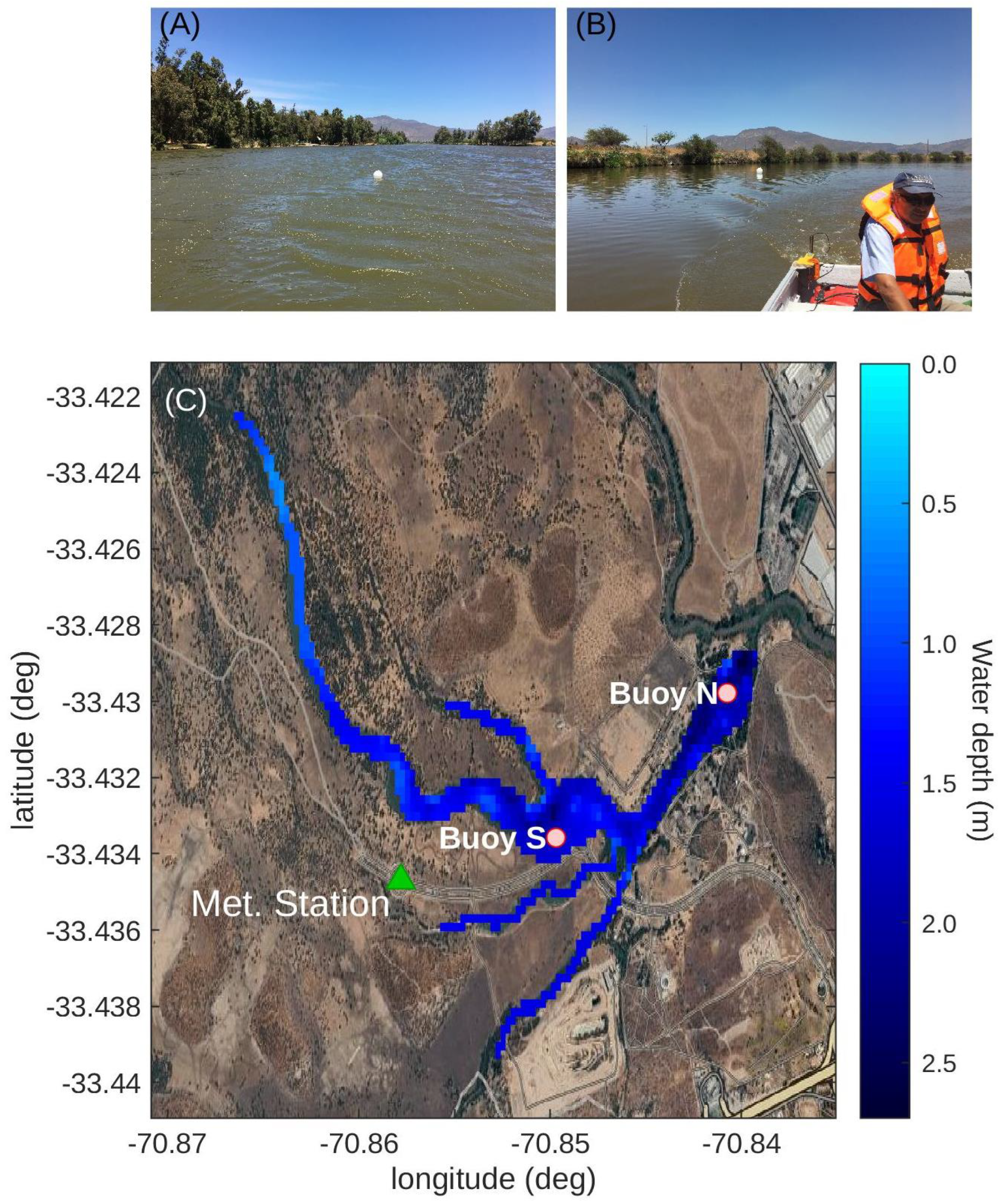
2.1. Study Site and Field Observations

Two limnological buoys have been recording vertical profiles of water temperature every 30 cm since 2016, although there have been periods with missing data that prevents computing, for example, the depth of the thermocline for the entire period of time. The buoys are designated as N (north) with nine thermistors and S (south) with five thermistors, with their locations indicated by red circles in Figure 1C. In this article, we will focus on the vertically averaged water temperature ($T_w$) and the maximum temperature difference in the vertical profile ($\Delta T_w$) used as a proxy for the stratification of the water column, and used by Holgerson et al. [4] for classifying the mixing regimes of shallow lakes. These time series are illustrated in Figure 2, where Figure 2A displays the vertically average water temperature for both buoys over the entire period, and Figure 2B shows the observed values of $\Delta T_w$ for the same period. Furthermore, Figure 2C presents the observed values of $\Delta T_w$ for a two-week period in 2018. During this time, the mixing regime of the shallow lake was characterized by well-mixed conditions with uniform water temperatures between 27 September and 30 September, followed by several days in which the maximum temperature was up to 10 °C higher than the minimum temperature observed during the day, while temperatures remained homogeneous at night.

Figure 2C also highlights significant differences between buoys N and S, with buoy S exhibiting weaker stratification (lower values of $\Delta T_w$) compared to buoy N. These differences can be attributed to the local water depth, which is 2.5 m for buoy N and 1.7 m for buoy S. Additionally, variations in the atmospheric boundary layer, influenced by the fetch length and sheltering from terrestrial vegetation, also play a role [29]. Buoy N is surrounded by tall trees (Figure 1A), while buoy S is located near the shore and surrounded by short bushes (Figure 1B). These factors, local water depth and atmospheric boundary layer, help to explain the primary differences observed in Figure 2.

Regarding the hydrology of the lake, it has two inflows and one outflow controlled by a spillway gate, which is opened sporadically. Information about the inflows and outflows is limited, characterized by sparse pulses of inflow volumes associated with surplus irrigation water entering the northern branch of the lake, as well as outflows from a small sewage treatment plant in the southern branch. Given these conditions, we estimated a retention time of one year [26]. Consequently, we assumed that both inflows and outflows are negligible, and that evaporation affects only the heat budget, not the water volume budget. Consequently, rainfall was also not included in the model, and the water level stayed constant during the entire simulation, with a small variation in the surface evalation range of 1 mm in the 50-years-long simulation.

2.2. Numerical Model

In this article, we employed a 3D numerical model to investigate the hydrodynamics of Laguna Carén (long: −70.8578; lat: −33.4347), a shallow reservoir with a maximum depth of 2.7 m, located near the capital of Chile [27]. The hydrodynamic model used is AEM3D from HydroNumerics Pty Ltd. (Brunswick, Australia), which is a parallel version of model ELCOM [13,30], and includes a heat sediment module designed to compute heat flux at the sediment–water interface (SWI) by solving the heat diffusion equation in the sediment. The AEM3D model solves the unsteady heat and momentum Reynolds-averaged hydrostatic equations in the horizontal dimensions, while the vertical transport of mass and momentum is addressed using a mixed-layer model as detailed by Hodges et al. [13]. This model computes the turbulent kinetic energy available for mixing and compares it with the energy required to mix two adjacent grid cells.

We utilized the model configuration established by Sáez et al. [27], dividing the domain into a uniform mesh grid with elements measuring 25 × 25 m in the horizontal direction and a vertical spacing of 20 cm (Figure 1C). In total, the lake is subdivided into 4277 wet points. Additionally, the heat sediment flux module was configured with 51 elements with variable vertical spacing: the first five elements below the SWI had a spacing of 1 cm, which then increased to 50 cm in the deepest element. Following Fang and Stefan [18], an adiabatic boundary condition can be applied at 12 m below the SWI, where the heat flux can be neglected. Finally, the bathymetry of the lake is assumed constant during the period of time, and to understand the long-term morphological changes in the shape of the lake is beyond the scope of this article.

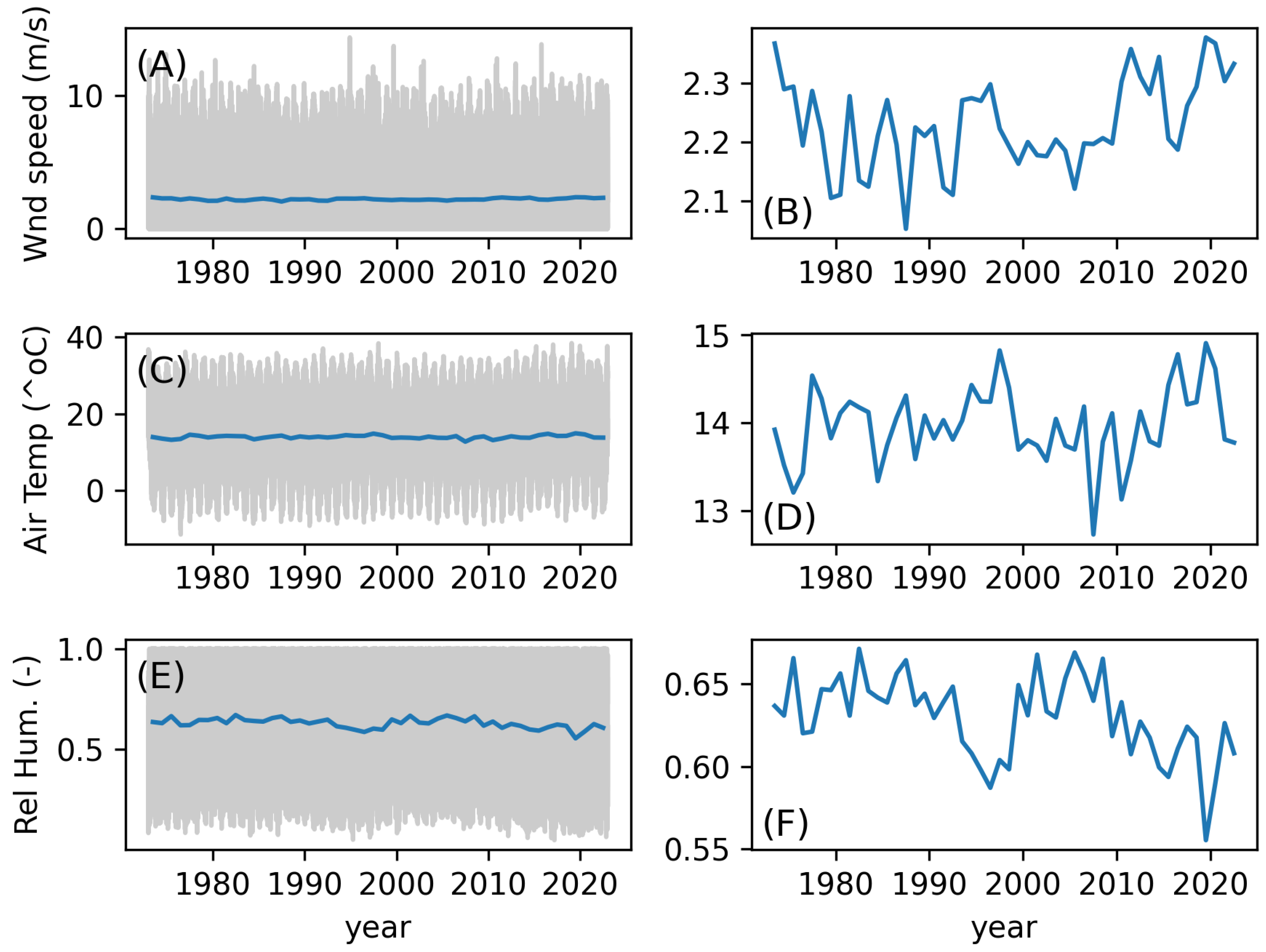
2.3. Meteorological Forcing

The green triangle in Figure 1 marks the location of the meteorological station, which collects data on wind speed and direction, air temperature and humidity, incident shortwave solar radiation, and atmospheric pressure. These observed meteorological data from the years 2017 to 2020 [27] were utilized to downscale the ERA5 reanalysis for the entire period from 1973 to 2022. To achieve this, we employed histogram equalization methods [31] for bias correction of the hourly ERA5 reanalysis data. As a result of this downscaling, Figure 3 presents the observed and corrected frequency distribution curves for wind speed, air temperature, and relative humidity. The close alignment of both curves supports the assertion that the corrected ERA5 meteorological information accurately represents local conditions in Laguna Carén. Following this downscaling, Figure 4 illustrates the time series of hourly meteorological forcing (left-hand column) and the annual averages (right-hand column).

2.4. Calibration of the Hydrodynamics Model

The calibration of the model focuses on the key parameters that significantly influence the hydrodynamics of the lake:

• Wind drag coefficient ($C_D$). This parameter determines the available turbulent kinetic energy for vertical mixing. The AEM3D model computes $C_D$ as a function of the atmospheric boundary layer stability, and it allows to specify the maximum value of $C_D$, which is considered constant and homogeneous over the lake surface and defines the surface roughness of the lake. For small lakes where the atmospheric boundary layer is not fully developed, values are typically smaller than 1.3 × ${10}^{-3}$.
• Light extinction coefficient, $k_l$, and albedo, $\alpha$. Both parameters affect light availability and penetration in the water column, depending on the lake’s trophic state. The light extinction coefficient ranges from 0.25 ${\mathrm{m}}^{-1}$ to 15 ${\mathrm{m}}^{-1}$ [4], while the surface albedo varies between 3% and 30% [32,33].
• Heat diffusion coefficient (${\kappa }_s$) and heat capacity of the sediment (${\left(\rho c_p\right)}_s$). These parameters control heat diffusion in the sediments. ${\kappa }_s$ can range between 0.01 and 0.11 ${\mathrm{m}}^2$⁄day, while ${\left(\rho c_p\right)}_s$ varies from 1.7 × ${10}^6$ to 3.8 × ${10}^6$ J/ ${\mathrm{m}}^{-3}$/°C [17,18].

To calibrate these parameters, simulations were conducted across a range of values for each parameter within their expected limits. For each simulation, time series data for vertically averaged water temperature ($T_w$) and the maximum temperature difference in the vertical profile ($\Delta T_w$) were generated. The agreement between the frequency distributions of the simulated values and observed values was assessed using the Kling–Gupta Efficiency (KGE) index [34]. This analysis was conducted for the hourly $T_w$ and $\Delta T_w$ data. The parameter combination associated with the minimum value of the product of the two KGE values was adopted for model calibration based on buoy N, with performance subsequently validated using buoy S observations.

2.5. Classification of the Mixing Regime

According to Holgerson et al. [4], the mixing regimes in shallow lakes can be classified based on the vertical gradient of the water density, estimated as the difference between the water density at the bottom and that at the surface, divided by the water depth. It was identified that if the vertical gradient of the water density exceeds 0.287 kg ${\mathrm{m}}^{-3}$ ${\mathrm{m}}^{-1}$, the water column is considered stratified. In this study, we adopted a uniform thermal expansion coefficient for water, making the threshold gradient of water density equivalent to a temperature gradient of 1.39 °C/m. Based on the local water depth, we define the water column as stratified if $\Delta T_w$ > 3.33 °C for buoy N and $\Delta T_w$ > 2.52 °C for buoy S. Using this definition, for each day, we calculated the fraction of the day during which the water column is stratified (hereafter referred to as $\%strat$). This index was averaged over the years or months to examine changes in the mixing regimes. Holgerson et al. [4] identified three mixing regimes with average $\%strat$ values of 98% for rarely mixed lakes, 74% for intermittently mixed water columns, and 25% for often-mixed water columns.

3. Results

3.1. Calibration and Validation

The calibration process resulted in the following combination of parameters: surface albedo of 9%, light extinction coefficient ($k_l$) of 3 ${\mathrm{m}}^{-1}$, wind drag coefficient ($C_D$) of 0.0004, heat diffusion coefficient (${\kappa }_s$) of 0.035 ${\mathrm{m}}^2$/day, and heat capacity of the sediment ${\left(\rho c_p\right)}_s$ at 2.3 × ${10}^6$ J/${\mathrm{m}}^3$/°C. The corresponding Kling–Gupta Efficiency (KGE) values for these parameters were 0.71 for $\Delta T_w$ and 0.79 for $T_w$, with the main results presented in Figure 5. Figure 5A,B compare the observed and simulated frequency distributions of $T_w$ for buoys N and S, respectively. For buoy N, the model accurately captures the frequency distribution of the observed $T_w$, while the model tends to overestimate the water temperatures in buoy S. The root mean square error, $rmse$, of $T_w$, of the simularion is equal to 1.32 °C and 2.16 °C in buoys N and S, respectively. The values of the $rmse$ in the other lakes are in the range of 0.5 to 2 °C [35]. Additionally, Figure 5C,D compares the observed and simulated values of $\Delta T_w$, showing that the model overestimates $\Delta T_w$ for buoy S but aligns well with the observed values for buoy N. Figure 5E,F plots the time series of the observed and simulated $\Delta T_w$ for the detailed period shown in Figure 2C. In summary, the model performs well in representing conditions observed in buoy N, but it tends to overestimate the water temperature and stratification for buoy S.

The sensitivity of the results to changes in the values of $C_D$ and ${\left(\rho c_p\right)}_s$ was analyzed. On the one hand, it is important to note that the model parameters were calibrated based on buoy N, suggesting that the spatial variability of these parameters may be significant, particularly for the wind drag coefficient. This is illustrated by the gray dashed lines, which show the results obtained with a wind drag coefficient of 0.006, highlighting the sensitivity of the model results to this parameter. Higher values of $C_D$ increase the turbulent kinetic energy available for mixing the water column (Figure 5C,D), while reducing the vertically averaged water temperature (Figure 5A,B). Consequently, the differences in model performance at buoys N and S may be attributed to the use of a homogeneous $C_D$, which could be inappropriate considering the impact of different terrestrial vegetation (Figure 1A,B) on wind sheltering over the lake. On the other hand, the solid gray lines in Figure 5 show the results obtained using a value of ${\left(\rho c_p\right)}_s=3.8\times {10}^6$ J/${\mathrm{m}}^3$/°C, quantifying the sensitivity of the results to changes in the magnitude of the heat flux exchanged between the water column and the sediments. Lower average water temperature values are obtained, and a larger value of ${\left(\rho c_p\right)}_s$ increases $\Delta T_w$, consistent with the findings of Sáez et al. [27].

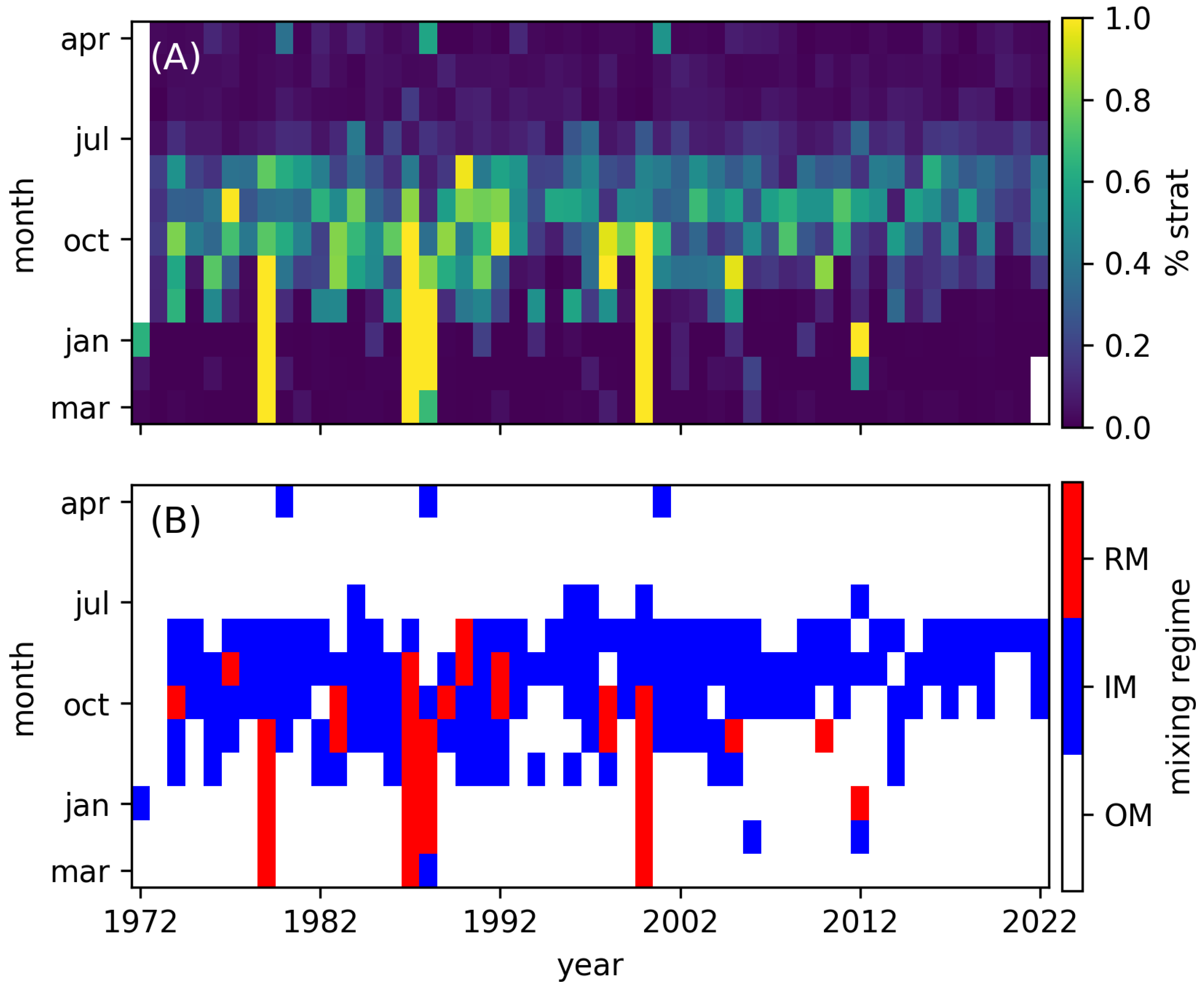
3.2. Annual Classification of Mixing Regimes

The characterization of mixing regimes in terms of annual averages of $\%strat$ is presented in Figure 6. Figure 6A,B plot the annual average simulated water temperature ($T_w$) for both buoys. The vertically average water temperature for buoy S is 18.2 ± 0.4 °C, while buoy N has an average of 17.5 ± 0.4 °C. No significant long-term changes in water temperature can be inferred from these results. However, Figure 6C,D illustrate the annual averages of $\Delta T_w$, revealing two distinct groups of years for buoy N. Most years exhibited a small average $\Delta T_w$ of 1.7 ± 0.4 °C, while four specific years, marked with red circles, showed a significant increase in average $\Delta T_w$ up to 6.2 ± 1.7 °C (Figure 6C). These peaks in $\Delta T_w$ correspond to changes in $\%strat$, which averaged 18.2 ± 5.9% for the majority of years, increasing to 57.2 ± 7.0% during the four years identified with red dots (Figure 6E). In contrast, buoy S displayed relatively constant $\Delta T_w$ and $\%strat$ values, averaging 14.8 ± 2.7%. In terms of the classifications defined by Holgerson et al. [4], the annual mixing regime for buoy S can be categorized as often mixed, while buoy N is predominantly often mixed in most years, though some years may be classified as intermittently mixed. Accordingly, the two groups of years are referred to as often-mixed years (OM years), with an average $\%strat$ of 19.7%, and intermittently mixed years (IM years), with an average $\%strat$ of 57.2%. Finally, the annual values of $\%strat$ exhibit a reduction in the last decade, when it takes values of 14.7 ± 5.2%, although the average $T_w$ has slightly increased to 17.6 ± 0.4 °C and $\Delta T_w$ reduced to 1.5 ± 0.3 °C.

The value of $\%strat$ exhibits significant seasonal variation that is hidden by the annual classification of mixing regimes. Figure 7 plots the monthly average $\%strat$, with filled areas indicating the range of values between the 16th and 84th percentiles. Figure 7A presents the results for buoy S, where $\%strat$ reaches its highest values in late winter and early spring (August and September), maintaining well-mixed conditions ($\%strat$ close to 0) for the rest of the year. On the contrary, buoy N (Figure 7B) shows significant differences between the two groups of years. In OM years, $\%strat$ increases from August to December (late winter and spring in the Southern Hemisphere) with minimal values during the remainder of the year. In contrast, the group of IM years deviates from this pattern beginning in September, when $\%strat$ begins to rise to 100% during late spring and in summer, classifying the water column as rarely mixed.

3.3. Influence of Meteorological Forcings on the Mixing Regime

In the previous section, we show that the annual mixing regimes simulated for buoy N in Laguna Carén exhibit two distinct groups of years: often-mixed (OM) and intermittently mixed (IM) years, each with differing seasonal patterns of $\%strat$. The results shown in Figure 7 reveal that both OM and IM years have similar $\%strat$ values between April and September but diverge significantly during the remaining months. Consequently, we explore which are the meteorological variables that play the most relevant role in determining the mixing regime for the remainder of spring and summer.

To investigate this correlation, we computed the average $\%strat$ for October and November alongside the average meteorological conditions for wind speed, air temperature, relative humidity, and cloud cover in the same months. We analyzed the daily maximum, daily minimum, and daily average values for these meteorological variables. Linear regression models were employed to establish relationships between these meteorological forcings and $\%strat$, with the coefficient of determination (${\mathrm{r}}^2$) serving as an indicator of the relevance of each factor in explaining $\%strat$. The coefficients from the regressions provide insights into the nature of these relationships.

These findings are summarized in

Table 1. Summary of statistical analysis for inferring the meteorological conditions that define the emergence of IM. years.

Variable	Agregation	Percentile	${\mathrm{r}}^2$	coef
		(%)	(-)	(-)
Wnd.speed	max	25	0.17	−0.23
Wnd.speed	min	21	0.14	−2.13
Wnd.speed	avg	21	0.21	−0.60
$T_a$	max	48	<0.01	0.00
$T_a$	min	53	0.02	0.05
$T_a$	avg	55	0.01	0.03
$cc$	max	53	<0.01	0.12
$cc$	min	47	<0.01	−0.16
$cc$	avg	56	<0.01	−0.02
$RH$	max	72	0.12	2.00
$RH$	min	70	0.13	1.62
$RH$	avg	73	0.14	1.68

, where the “Percentile” column reflects the average percentile of the IM years based on the calculated averages for October and November. The results indicate that wind speed is the most dominant meteorological factor influencing $\%strat$. Specifically, the average wind speed in October and November accounts for 21% of the variance in $\%strat$ during October and November, thereby explaining most of the meteorological differences between IM and OM years. For the wind speed, the coefficients of the linear regressions are negative, indicating that higher wind speeds correlate with lower $\%strat$. This aligns with the understanding that wind is the primary source of turbulent kinetic energy available for mixing in the water column; therefore, increased wind leads to greater mixing and a reduction in $\%strat$. Furthermore, IM years are associated with lower wind percentages, suggesting that these years occur when winds in October and November are weak. Although the remaining variables exhibited lower ${\mathrm{r}}^2$ values, the interpretation of the percentiles indicates that IM years are generally cooler with higher relative humidity.

However, the previously described correlations between meteorological variables and $\%strat$ exhibit seasonal variation. This is illustrated in Figure 8, which plots the ${\mathrm{r}}^2$ values obtained from linear regressions between the meteorological variables and $\%strat$ for the different months of the year. Figure 8A indicates that wind speed is a relevant variable for explaining $\%strat$ during most of the rear but in autum, with peak values of ${\mathrm{r}}^2$ values of around 0.2 for the months of October and November. The air temperature is more significant during late winter and early spring (Figure 8B), while the cloud cover of Figure 8C did not display either notable seasonal fluctuations or relevance in statistically explaining $\%strat$. Finally, the relative humidity is a relevant factor in October–November (Figure 8D).

Finally, the correlation between wind speed and mixing regimes in Laguna Carén of Table 1 helps to explain the reduction in the annual $\%strat$ that was presented in Figure 6 during the last decade. In particular, Figure 4B showed that the annual average wind increases from 2.2 m/s before 2010, up to 2.3 m/s after 2010, and this increase in the annual average wind explains the reduction in $\%strat$. Furthermore, Figure 9 plots the time series of the annual wind energy that is available for mixing the water column that shows an increase over the time at a rate equal to 0.13% per decade. The wind energy was computed following Wüest et al. [36] as

$$E=\int {\rho }_a{C}_D{U}_{wnd}^{3}dt$$

(1)

where ${\rho }_a$ is the air density and $U_{wnd}$ the wind speed.

3.4. Monthly Classifying of Mixing Regimes

So far, we have shown that the classification of the mixing regimes in buoy N depends on the season of the year and the external meteorological forcings. While the differentiation between intermittently mixed (IM) and often-mixed (OM) years is evident based on the annual values presented in Figure 6, it remains unclear whether it is possible to distinguish between mixing regimes at a monthly timescale. Figure 10 illustrates the frequency distribution of $\%strat$ for all months across both buoys. From this figure, no clear threshold values emerge to differentiate between the three mixing regimes identified by Holgerson et al. [4]. Therefore, we adopted round values of 20% to distinguish between OM and IM regimes, and 80% to differentiate between IM and rarely mixed (RM) regimes, as shown in Figure 10. Based on these threshold values, we classified the mixing regimes at a monthly timescale, with the results illustrated in Figure 11 for buoy S and Figure 12 for buoy N. In Figure 11 and Figure 12, panel A displays a year-month heatmap of $\%strat$ for all months and years within the 50-year simulation, while panel B shows the associated mixing regime.

Regarding buoy S, as noted in Figure 7, the water column exhibits stratification for a fraction of the day during late winter and spring, with less than 50% of the day classified as stratified (Figure 11B). In terms of the mixing regime, the water column is typically categorized as often mixed, and occasionally classified as intermittently mixed for just a couple of months each year (Figure 11B). The water depth at buoy S is 1.7 m, which contrasts with buoy N, where the local water depth is 2.5 m, leading to substantial differences in mixing regime classification.

Figure 12B reveals that the mixing regime for buoy N predominantly reflects OM or IM (red and blue areas), with instances of classification as rarely mixed (RM) not only during the summer months of recognized IM years, as identified in Figure 6, but also during certain other months. Wind speed is one of the factors that can explain the existence of months where the water column rarely mixes; however, the statistical exploration of the previous section indicates that it can explain at most 25% of the variance of the $\%strat$. This highlights the need for further detailed investigations into the factors influencing these observations.

Finally, the reduction in $\%strat$ simulated over the last decade has also affected the monthly classification of mixing regimes for both buoys. The number of months classified as intermittently mixed (IM) has significantly decreased in recent years for both buoys. In buoy N, the months classified as rarely mixed (RM) have been reduced to zero, while the number of months categorized as IM has decreased to just one when compared to values from the previous century.

4. Discussion

4.1. Hydrodynamics Simulation of Shallow Lakes

In this article, we presented the results of a 50-year hydrodynamic simulation of Laguna Carén, a shallow lake located near the capital city of Chile. The simulation utilized the AEM3D hydrodynamic model, which can simulate the key processes necessary to represent the stratification and mixing of the water column that define the mixing regime of shallow lakes. These processes include heat and momentum exchanges with the atmosphere, light penetration into the water column, and heat diffusion in the sediments affecting heat exchanges across the sediment-water interface. Furthermore, the use of a 3D model enables the representation of horizontal currents that can be generated by differential water temperatures in the lake [35], such as cold ponds that may form in the deepest areas, thus contributing to the stratification of the water column. The parameters controlling these processes were calibrated based on the field observations and were assumed to remain constant and uniform throughout the 50-year simulation. However, this assumption of constant and homogeneous coefficients may not always hold true. For instance, the light extinction coefficient is influenced by water turbidity (suspended solids and algae concentration) [37], which varies seasonally and is affected by the trophic state of the lake, the occurrence of algae blooms, nutrient concentration, fertilizers, terrestrial vegetation, and many other factors [38,39]. Therefore, seasonal variations in algae concentration and/or long-term changes in the trophic state of the lake could significantly impact the mixing regimes of the shallow lake. Further research is necessary to quantify the connections and feedback loops between mixing regimes and the ecology of shallow lakes.

Additionally, the AEM3D model computes heat and momentum exchanges between the atmosphere and the lake as a function of the atmospheric boundary layer stability, and the calibrated $C_D$ = 0.0004 is used by the model to specify the surface roughness, which is homogeneous across the entire lake. This assumption does not accurately reflect the development of the atmospheric boundary layer over the water body, which can be affected by proximity to the shore and surrounding terrestrial vegetation (Figure 1A,B). This could explain the issues with validation of the model in buoy S, where it overestimated both $T_w$ and $\Delta T_w$. Increasing the calibrated value of the wind drag coefficient ($C_D$) would increase the turbulent kinetic energy available for mixing, thereby reducing $\Delta T_w$, as shown in Figure 5C,D [12,36]. A higher $C_D$ would also enhance latent and sensible heat fluxes, decreasing the temperature difference between the air and water needed to balance heat fluxes across the air–water interface [19]. However, while using a larger $C_D$ could improve model performance at buoy S, it may degrade performance for buoy N (see gray lines in Figure 5). Therefore, our results shows that a better representation of the atmospheric boundary layer dynamics is needed to correctly represents spatial differences in the observed water temperature. Finally, the adopted model includes the heat flux exchanged between the water column and the sediment, and the sensitivity results shown in Figure 5 indicate that this flux can enhance the stratification [27], as the simulated values of $\Delta T_w$ increase in the simulation where a higher value of ${\left(\rho c_p\right)}_s$ was used.

4.2. Wind Speed

Climate change is typically associated with rising air temperatures (average and heat waves) and alterations in precipitation patterns (in terms of amount and timing) due to increased atmospheric concentrations of greenhouse gases [40,41,42]. However, there has been relatively less focus on the impact of other meteorological variables that are critical for the energy balance at the air–water interface, including wind speed, cloud cover, and air moisture. One of the main contributions of this article is to highlight the significant role of wind speed in the stratification and mixing of the water column in the context of climate change. Wind speed influences energy balance at the air–water interface by controlling sensible and latent heat fluxes, which generally counteract incident shortwave radiation [20,43]. Increased wind speeds necessitate smaller temperature differences between air and water, while also amplifying evaporative losses [21].

In the context of stratification and mixing processes in shallow lakes, wind speed, alongside the wind drag coefficient, dictates the amount of turbulent kinetic energy available for total or partial mixing of the water column [36]. Consequently, a reduction in wind speed may lead to changes in mixing regimes, with an increased fraction of time during which the water column stratifies. The ecological implications of these hydrodynamic changes in water bodies are not fully understood, warranting further analysis to evaluate, for example, how variations in mixing regimes affect dissolved oxygen concentrations in shallow lakes.

Our findings indicate that wind speed is the most relevant variable in explaining the emergence of the IM years of Figure 7. The mixing regime during often-mixed (OM) years is maintained by sufficiently high wind speeds; these conditions effectively mix the water column and prevent the establishment of stable stratification. This correlation is particularly significant in October and November (Figure 8A), coinciding with the onset of intermittently mixed (IM) years (Figure 7B). Conversely, the emergence of IM years appears to be linked to reduced wind speeds in spring and summer. Unfortunately, field observations of IM years are lacking, highlighting the need for validation of this phenomenon.

The 50-year simulation also showed a shift in the mixing regime of the shallow lake toward less stratified conditions, which can also be attributed to changes in wind speed. Specifically, Figure 9 demonstrates that annual wind energy has increased over time, which is consistent with the reduction in the fraction of time during which the water column is stratified. However, it is important to note that stratification also depends on air temperature, a meteorological variable that has not shown significant changes in the available records in the region [40], and it is unclear how the increase in the air temperature will interact with changes in the wind speed.

4.3. Spatial Differences in the Mixing Regime

Finally, beyond differences in wind sheltering related to terrestrial vegetation, the variations in the mixing regimes of buoys S and N can be attributed to the local depth, which measures 1.7 m for buoy S and 2.5 m for buoy N. In the context of the Monin–Obukhov length (ℓ), defined as [6,44]

$$\ell ={\displaystyle \frac{u_{*}^3}{B}}$$

(2)

where $u_{*}$ represents the wind shear velocity and B denotes the buoyancy flux associated with heat exchanges at the AWI. ℓ is typically understood as the depth scale over which wind mixing counterbalances the potential energy gained from surface heating [45]. This depth can indicate the extent of mixing in a water column that is consistently stratified by B.

In shallow lakes, ℓ can be greater or smaller than the local depth: where the local depth is greater than ℓ, the water column tends to stratify, while where it is smaller, the water column remains well mixed. This relationship primarily explains the differing mixing regimes between buoy S and buoy N in relation to their respective local water depths. However, further theoretical and experimental studies are necessary to determine how to incorporate heat flux across the sediment–water interface when estimating B, and how the Monin–Obukhov length can be applied to delineate zones within shallow lakes.

4.4. Climate Change Simulations

The 50-years-long simulation showed the emergence of IM years in the last century, and a reduction in the $\%strat$ in the last decade with the corresponding reduction of the months per year when the mixing regime is classified as IM or RM. In this context, the presented model can be utilized to define whether changes in the mixing regime of shallow lakes can be attributed to climate change. This evaluation requires downscaling the meteorological forcings from various SSP-RCP models of the CMIP6 [46] to the local conditions of Laguna Carén [47,48,49]. However, future projections of meteorological conditions are typically available on a daily timescale and often lack detail regarding sub-daily cycles of wind speed and other necessary meteorological information for modeling. Addressing this limitation is crucial prior to conducting climate change simulations in shallow lakes, as the turbulent kinetic energy available for mixing is dependent on the square of the wind speed [36] and the Monin–Obukhov length is proportional to the wind shear velocity to the power of 3. Consequently, the turbulent kinetic energy and ℓ associated with a constant wind equal to the average wind speed will be less than that of a variable wind speed throughout the day. Once this first limitation is resolved, it will be possible to determine whether changes in the mixing regime are expected in response to the different SSP-RCP scenarios.

5. Conclusions

The numerical results presented in this article enable the conclusion that the mixing regime in shallow lakes is not constant over time; rather, it can exhibit emergence of years characterized by changes in mixing regimes and decadal changes in $\%strat$. These variations in the mixing regime were attributed to alterations in meteorological forcing, particularly wind speed, which plays a crucial role in determining the turbulent kinetic energy available for mixing the water column [36]. As wind speeds increase, the potential for mixing rises accordingly. Conversely, a reduction in wind speed may lead to prolonged periods of stable stratification of the water column.

Although this study did not examine the relationship between the mixing regime and the ecology of the shallow lake, it is possible to speculate that alterations in mixing dynamics could have unpredictable consequences for the ecology of the lake. Future research is required to explore these ecological implications and to better understand the links between hydrodynamics and the ecology of shallow lakes.

References

1. Cole, J.J.; Prairie, Y.T.; Caraco, N.F.; McDowell, W.H.; Tranvik, L.J.; Striegl, R.G.; Duarte, C.M.; Kortelainen, P.; Downing, J.A.; Middelburg, J.J.; et al. Plumbing the global carbon cycle: Integrating inland waters into the terrestrial carbon budget. Ecosystems 2007, 10, 171–184. [Google Scholar] [CrossRef]
2. Tranvik, L.J.; Downing, J.A.; Cotner, J.B.; Loiselle, S.A.; Striegl, R.G.; Ballatore, T.J.; Dillon, P.; Finlay, K.; Fortino, K.; Knoll, L.B.; et al. Lakes and reservoirs as regulators of carbon cycling and climate. Limnol. Oceanogr. 2009, 54, 2298–2314. [Google Scholar] [CrossRef]
3. Strassburg, B.B.; Iribarrem, A.; Beyer, H.L.; Cordeiro, C.L.; Crouzeilles, R.; Jakovac, C.C.; Junqueira, A.B.; Lacerda, E.; Latawiec, A.E.; Balmford, A.; et al. Global priority areas for ecosystem restoration. Nature 2020, 586, 724–729. [Google Scholar] [CrossRef]
4. Holgerson, M.A.; Richardson, D.C.; Roith, J.; Bortolotti, L.E.; Finlay, K.; Hornbach, D.J.; Gurung, K.; Ness, A.; Andersen, M.R.; Bansal, S.; et al. Classifying Mixing Regimes in Ponds and Shallow Lakes. Water Resour. Res. 2022, 58, e2022WR032522. [Google Scholar] [CrossRef]
5. Davidson, T.A.; Søndergaard, M.; Audet, J.; Levi, E.; Esposito, C.; Bucak, T.; Nielsen, A. Temporary stratification promotes large greenhouse gas emissions in a shallow eutrophic lake. Biogeosciences 2024, 21, 93–107. [Google Scholar] [CrossRef]
6. Masunaga, E.; Komuro, S. Stratification and mixing processes associated with hypoxia in a shallow lake (Lake Kasumigaura, Japan). Limnology 2020, 21, 173–186. [Google Scholar] [CrossRef]
7. Adrian, R.; O’Reilly, C.M.; Zagarese, H.; Baines, S.B.; Hessen, D.O.; Keller, W.; Livingstone, D.M.; Sommaruga, R.; Straile, D.; Donk, E.V.; et al. Lakes as sentinels of climate change. Limnol. Oceanogr. 2009, 54, 2283–2297. [Google Scholar] [CrossRef] [PubMed]
8. Williamson, C.E.; Saros, J.E.; Vincent, W.F.; Smol, J.P. Lakes and reservoirs as sentinels, integrators, and regulators of climate change. Limnol. Oceanogr. 2009, 54, 2273–2282. [Google Scholar] [CrossRef]
9. Bouffard, D.; Wüest, A. Convection in Lakes. Annu. Rev. Fluid Mech. 2019, 51, 189–215. [Google Scholar] [CrossRef]
10. Fischer, H.; List, R.; Imberger, J.; Brooks, N. Mixing in Island and Coastal Waters; Academic Press: Cambridge, MA, USA, 1979. [Google Scholar]
11. Imberger, J. Environmental Fluid Dynamics; Academic Press: Cambridge, MA, USA, 2013. [Google Scholar] [CrossRef]
12. Wüest, A.; Lorke, A. Small-Scale Hydrodynamics in Lakes. Annu. Rev. Fluid Mech. 2003, 35, 373–412. [Google Scholar]
13. Hodges, B.R.; Imberger, J.; Saggio, A.; Winters, K.B. Modeling basin-scale internal waves in a stratified lake. Limnol. Oceanogr. 2000, 45, 1603–1620. [Google Scholar] [CrossRef]
14. Ivey, G.N.; Winters, K.B.; Koseff, J.R. Density stratification, turbulence, but how much mixing? Annu. Rev. Fluid Mech. 2008, 40, 169–184. [Google Scholar]
15. Winters, K.B.; Lombard, P.N.; Riley, J.J.; D’Asaro, E.A. Available potential energy and mixing in density-stratified fluids. J. Fluid Mech. 1995, 289, 115. [Google Scholar] [CrossRef]
16. Ulloa, H.N.; Wüest, A.; Bouffard, D. Mechanical energy budget and mixing efficiency for a radiatively heated ice-covered waterbody. J. Fluid Mech. 2018, 852, R1–R13. [Google Scholar] [CrossRef]
17. Fang, X.; Stefan, H.G. Dynamics of heat exchange between sediment and water in a lake. Water Resour. Res. 1996, 32, 1719–1727. [Google Scholar] [CrossRef]
18. Fang, X.; Stefan, H.G. Temperature Variability in Lake Sediments. Water Resour. Res. 1998, 34, 717–729. [Google Scholar]
19. Csanady, G.; Lumley, J. Air-Sea Interaction: Laws and Mechanisms. Appl. Mech. Rev. 2002, 55, 1508156. [Google Scholar] [CrossRef]
20. Garratt, J.R. The Atmospheric Boundary Layer; Cambridge University Press: Cambridge, UK, 1992. [Google Scholar]
21. de la Fuente, A.; Meruane, C. Spectral model for long-term computation of thermodynamics and potential evaporation in shallow wetlands. Water Resour. Res. 2017, 53, 7696–7715. [Google Scholar] [CrossRef]
22. Woolway, R.I.; Sharma, S.; Weyhenmeyer, G.A.; Debolskiy, A.; Golub, M.; Mercado-Bettín, D.; Perroud, M.; Stepanenko, V.; Tan, Z.; Grant, L.; et al. Phenological shifts in lake stratification under climate change. Nat. Commun. 2021, 12, 19. [Google Scholar] [CrossRef]
23. Piccioni, F.; Casenave, C.; Lemaire, B.J.; Moigne, P.L.; Dubois, P.; Vinçon-Leite, B. The thermal response of small and shallow lakes to climate change: New insights from 3D hindcast modelling. Earth Syst. Dyn. 2021, 12, 439–456. [Google Scholar] [CrossRef]
24. de la Fuente, A.; Meruane, C. Dimensionless numbers for classifying the thermodynamics regimes that determine water temperature in shallow lakes and wetlands. Environ. Fluid Mech. 2017, 17, 1081–1098. [Google Scholar] [CrossRef]
25. Martinsen, K.T.; Andersen, M.R.; Sand-Jensen, K. Water temperature dynamics and the prevalence of daytime stratification in small temperate shallow lakes. Hydrobiologia 2019, 826, 247–262. [Google Scholar] [CrossRef]
26. Aranguiz, C. Estudio e Identificación de los Procesos bioquíMicos Asociados a los Nutrientes N y P en Interacción con el ciclo del Carbono. Caso de Estudio: Laguna Carén, Chile. Undergraduate Thesis, Universidad de Chile, Santiago, Chile, 2019. Available online: https://repositorio.uchile.cl/handle/2250/171000 (accessed on 27 March 2024). (In Spanish).
27. Sáez, B.; Boegman, L.; Olshoorn, J.; de la Fuente, A. A model of stratification and mixing in a shallow lake with heat flux at the sediment-water interface: Application to Laguna Carén. J. Geophys. Res. 2025, submit. [Google Scholar]
28. Hersbach, H.; Bell, B.; Berrisford, P.; Hirahara, S.; Horányi, A.; Muñoz-Sabater, J.; Nicolas, J.; Peubey, C.; Radu, R.; Schepers, D.; et al. The ERA5 global reanalysis. Q. J. R. Meteorol. Soc. 2020, 146, 1999–2049. [Google Scholar] [CrossRef]
29. Markfort, C.D.; Porté-Agel, F.; Stefan, H.G. Canopy-wake dynamics and wind sheltering effects on Earth surface fluxes. Environ. Fluid Mech. 2014, 14, 663–697. [Google Scholar] [CrossRef]
30. Hodges, B.; Dallimore, C. Estuary, Lake and Coastal Ocean Model: ELCOM v2. 2 User Manual; Centre for Water Research, The University of Western Australia: Crawley, Australia, 2010. [Google Scholar]
31. Maraun, D.; Wetterhall, F.; Ireson, A.M.; Chandler, R.E.; Kendon, E.J.; Widmann, M.; Brienen, S.; Rust, H.W.; Sauter, T.; Themel, M.; et al. Precipitation downscaling under climate change: Recent developments to bridge the gap between dynamical models and the end user. Rev. Geophys. 2010, 48, 2009RG000314. [Google Scholar] [CrossRef]
32. Du, J.; Jacinthe, P.A.; Song, K.; Zhou, H. Water surface albedo and its driving factors on the turbid lakes of Northeast China. Ecol. Indic. 2023, 146, 109905. [Google Scholar] [CrossRef]
33. Du, J.; Zhou, H.; Jacinthe, P.A.; Song, K. Retrieval of lake water surface albedo from Sentinel-2 remote sensing imagery. J. Hydrol. 2023, 617, 128904. [Google Scholar] [CrossRef]
34. Gupta, H.V.; Kling, H.; Yilmaz, K.K.; Martinez, G.F. Decomposition of the mean squared error and NSE performance criteria: Implications for improving hydrological modelling. J. Hydrol. 2009, 377, 80–91. [Google Scholar] [CrossRef]
35. Zhou, W.; Melack, J.M.; MacIntyre, S.; Barbosa, P.M.; Amaral, J.H.; Cortés, A. Hydrodynamic Modeling of Stratification and Mixing in a Shallow, Tropical Floodplain Lake. Water Resour. Res. 2024, 60, e2022WR034057. [Google Scholar] [CrossRef]
36. Wüest, A.; Piepke, G.; Senden, D.V. Turbulent kinetic energy balance as a tool for estimating vertical diffusivity in wind-forced stratified waters. Limnol. Oceanogr. 2000, 45, 1388–1400. [Google Scholar] [CrossRef]
37. Devlin, M.J.; Barry, J.; Mills, D.K.; Gowen, R.J.; Foden, J.; Sivyer, D.; Greenwood, N.; Pearce, D.; Tett, P. Estimating the diffuse attenuation coefficient from optically active constituents in UK marine waters. Estuarine, Coast. Shelf Sci. 2009, 82, 73–83. [Google Scholar] [CrossRef]
38. Mitsch, W.J.; Gosselink, J.G. Wetlands, 5th ed.; John Wiley & Sons: Hoboken, NJ, USA, 2015; Volume 91. [Google Scholar]
39. Wetzel, R.G. Limnology: Lake and River Ecosystems; Academic Press: Cambridge, MA, USA, 2001; p. 1006. [Google Scholar]
40. Lagos-Zúñiga, M.; Mendoza, P.A.; Campos, D.; Rondanelli, R. Trends in seasonal precipitation extremes and associated temperatures along continental Chile. Clim. Dyn. 2024, 62, 4205–4222. [Google Scholar] [CrossRef]
41. González-Reyes, A.; Jacques-Coper, M.; Bravo, C.; Rojas, M.; Garreaud, R. Evolution of heatwaves in Chile since 1980. Weather Clim. Extrem. 2023, 41, 100588. [Google Scholar] [CrossRef]
42. Feron, S.; Cordero, R.R.; Damiani, A.; Oyola, P.; Ansari, T.; Pedemonte, J.C.; Wang, C.; Ouyang, Z.; Gallo, V. Compound climate-pollution extremes in Santiago de Chile. Sci. Rep. 2023, 13, 6726. [Google Scholar] [CrossRef]
43. Stull, R.B. An Introduction to Boundary Layer Meteorology; Springer Dordrecht: Dordrecht, The Netherlands, 1988; Volume 13, p. 666. [Google Scholar]
44. Monin, A.S.; Obukhov, A.M. Basic laws of turbulent mixing in the atmosphere near the ground. Tr. Akad. Nauk SSSR Geofiz. Inst 1954, 24, 163r187. [Google Scholar]
45. Imberger, J. The diurnal mixed layer. Limnol. Oceanogr. 1985, 30, 737–770. [Google Scholar] [CrossRef]
46. Eyring, V.; Bony, S.; Meehl, G.A.; Senior, C.A.; Stevens, B.; Stouffer, R.J.; Taylor, K.E. Overview of the Coupled Model Intercomparison Project Phase 6 (CMIP6) experimental design and organization. Geosci. Model Dev. 2016, 9, 1937–1958. [Google Scholar] [CrossRef]
47. Cannon, A.J. Multivariate quantile mapping bias correction: An N-dimensional probability density function transform for climate model simulations of multiple variables. Clim. Dyn. 2018, 50, 31–49. [Google Scholar] [CrossRef]
48. Piccolroaz, S.; Zhu, S.; Ladwig, R.; Carrea, L.; Oliver, S.; Piotrowski, A.P.; Ptak, M.; Shinohara, R.; Sojka, M.; Woolway, R.I.; et al. Lake Water Temperature Modeling in an Era of Climate Change: Data Sources, Models, and Future Prospects. Rev. Geophys. 2024, 62, e2023RG000816. [Google Scholar] [CrossRef]
49. de la Fuente, A.; Meruane, C.; Meruane, V. Expected reliability over a planning horizon of a hydraulic infrastructure and its uncertainty under hydroclimatic future projections. J. Hydrol. 2023, 622, 129700. [Google Scholar] [CrossRef]
Figure 1. (A) Location of buoy N. (B) location of buoy S. (C) Bathymetry of Carén, and location of buoys N and S, with the meteorological station marked with a green triangle.
Water 17 01007 g001
Figure 2. Field observations in buoy N (blue) and S (red) of (A) the vertically average water temperature ( T w ) and (B) the maximum water temperature difference in the vertical profile ( Δ T w ). (C) Detailed view of (B) for the period of time between 27 September and 8 October of 2018.
Water 17 01007 g002
Figure 3. Comparison between frequency distribution curves of the observed (dashed line) and downscaled meteorological forcing of the model for (A) wind speed, (B) air temperature, and (C) relatively humidity.
Water 17 01007 g003
Figure 4. Time series of meteorological forcings to the model. Left-hand-side plots the hourly information (A,C,E) and the right-hand-side column, the annual value (B,D,F). First row corresponds to the wind speed, second row to the air temperature, and third row corresponds to the relative humidity.
Water 17 01007 g004
Figure 5. Calibration and validation of the model. (A,B) compare the frequency distribution of the observed and simulated T w for buoys N and S, respectively. (C,D) compare the frequency distribution of the observed and simulated Δ T w . (E,F) plot the observed and simulated time series of Δ T w for the time period between 27 September and 8 October of 2018. Grey dashed lines correspond to a simulation with a drag coefficient equal to 0.006, and grey solid lines correspond to a simulation with ( ρ c p ) s = 3.8 × 10 6 J/ m 3 /°C.
Water 17 01007 g005
Figure 6. Time series of annual average results in buoys N (left-hand-side panels) and S (right-hand-side panels) of (A,B) vertically average water temperature ( T w ), (C,D) difference between maximum and minimum temperatures for each profile ( Δ T w ), (E,F) time series of the annual value of % s t r a t .
Water 17 01007 g006
Figure 7. Monthly average value of % s t r a t for the two groups of year identified in Figure 6. (A) buoy S and (B) buoy N.
Water 17 01007 g007
Figure 8. Seasonal variation in r 2 for the linear regressions between the daily average meteorological variables and % s t r a t for the corresponding month.
Water 17 01007 g008
Figure 9. Time series of the annual wind energy that is available for mixing.
Water 17 01007 g009
Figure 10. Frequency distribution of % s t r a t for buoys N and S, and definition of threshold of % s t r a t for classification of mixing regimes based on monthly average values of % s t r a t .
Water 17 01007 g010
Figure 11. (A) Year-month heatmap of % s t r a t in buoy S. (B) Year-month heatmap of mixing regime in buoy S. Note that the horizontal axis starts in April.
Water 17 01007 g011
Figure 12. (A) Year-month heatmap of % s t r a t in buoy N. (B) Year-month heatmap of mixing regime in buoy N. Note that the horizontal axis starts in April.
Water 17 01007 g012