
Key Calibration Strategies for Mitigation of Water Scarcity in the Water Supply Macrosystem of a Brazilian City

 , ,
, ,  and
and 
Abstract
:1. Introduction
2. Materials and Methods
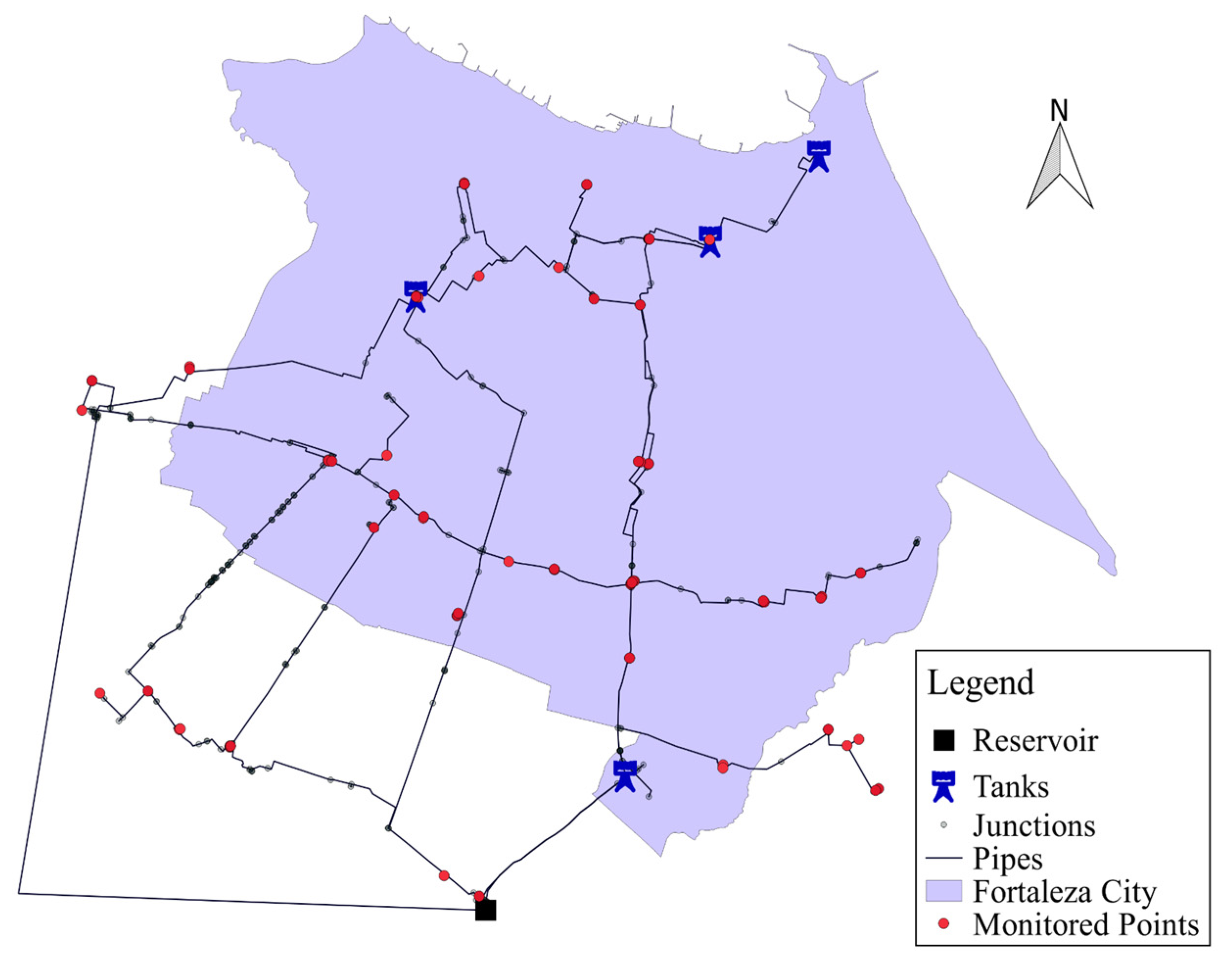
2.1. Study Area
2.2. Macrosystem of the Metropolitan Region of Fortaleza (MMF)
2.3. Methodology
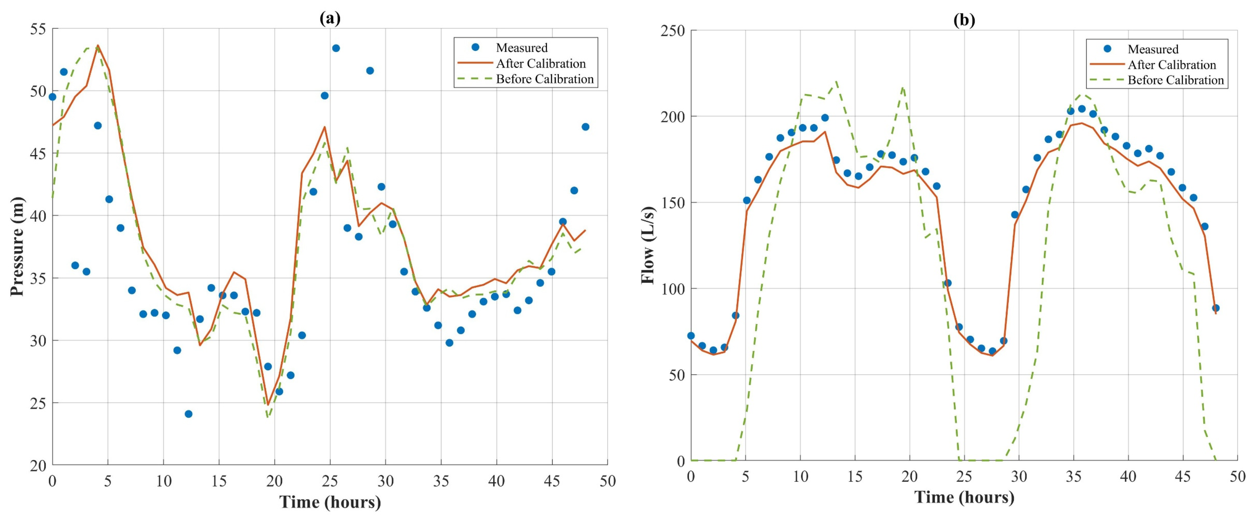
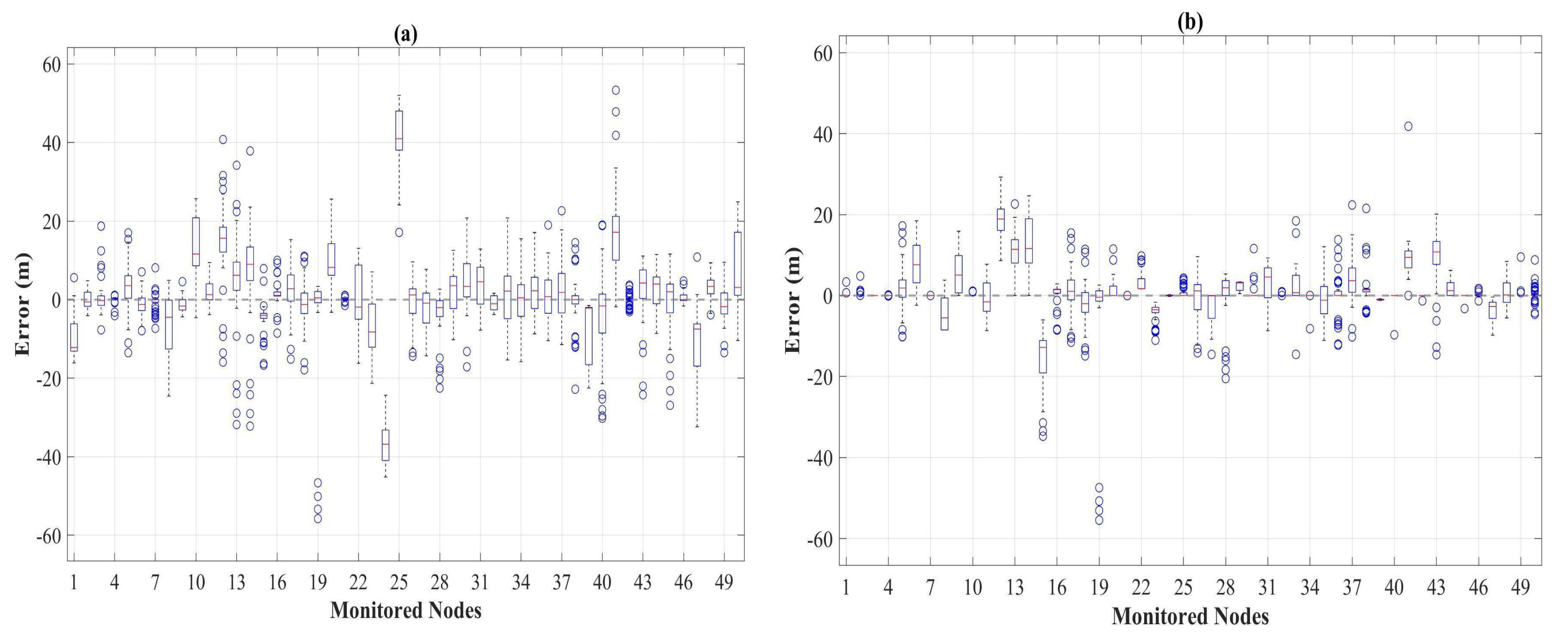
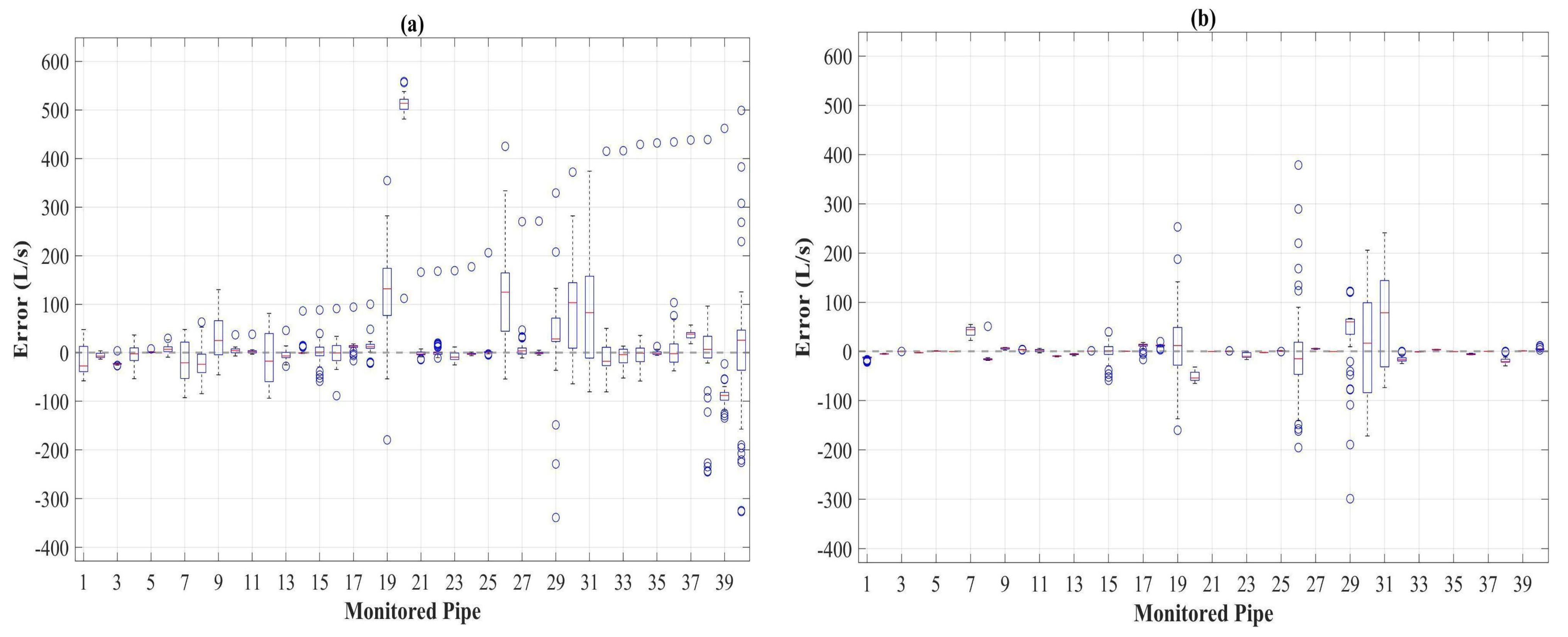
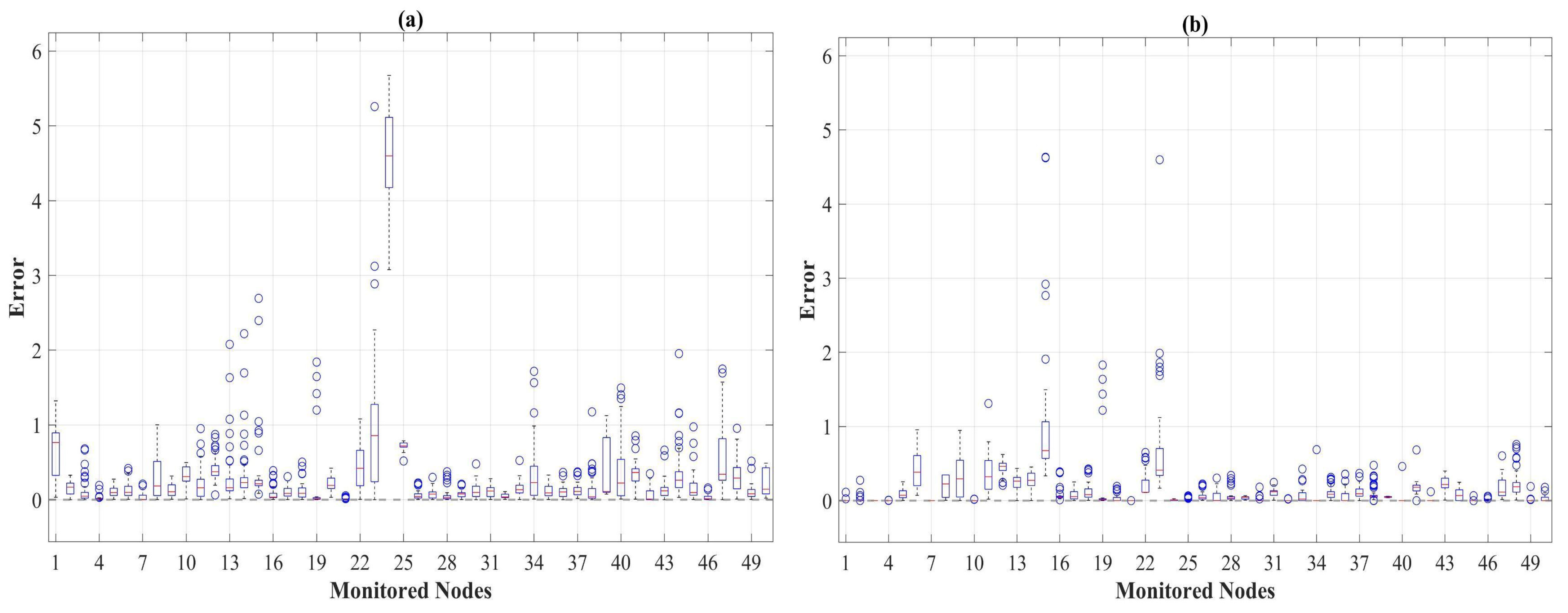
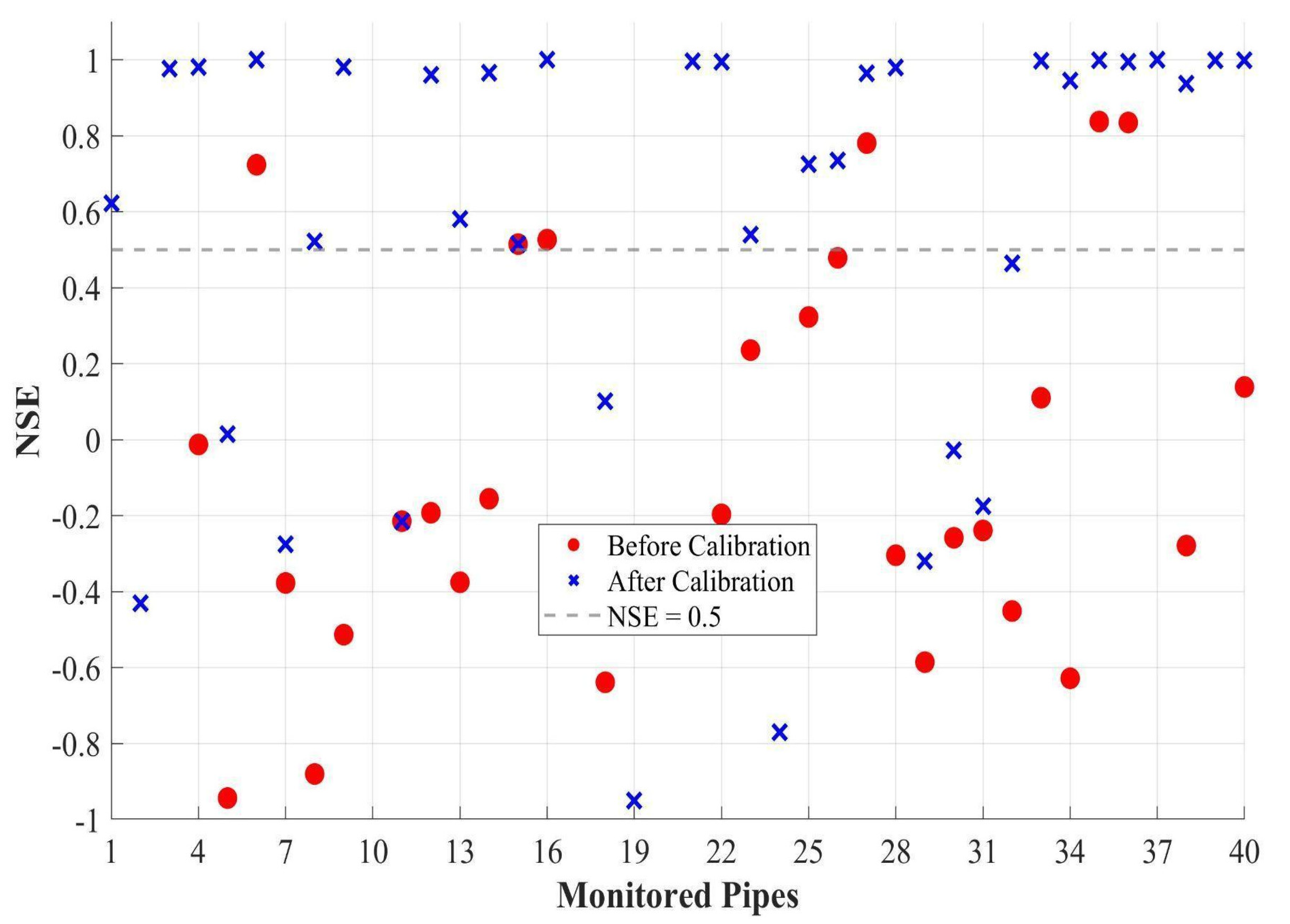
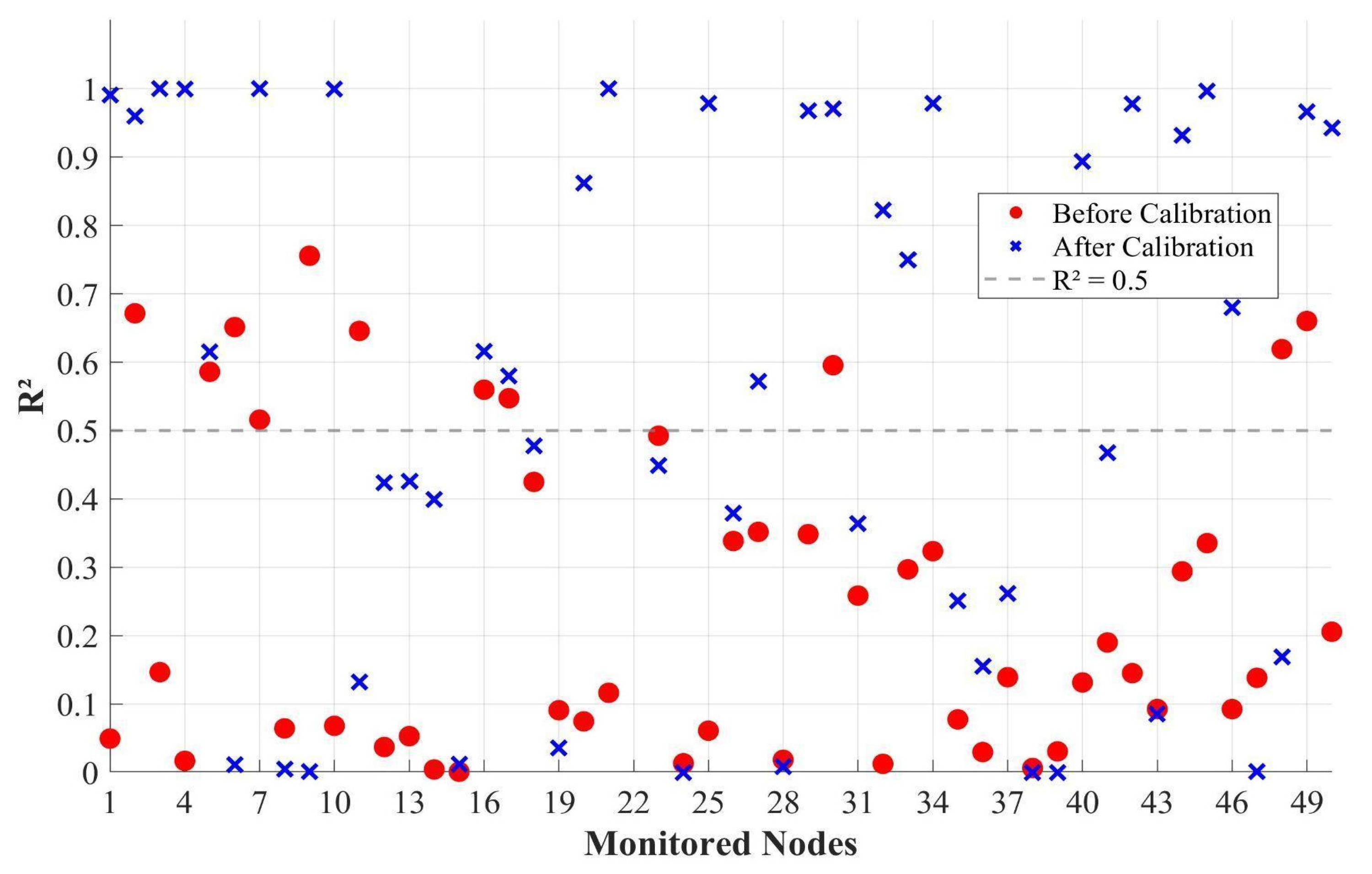
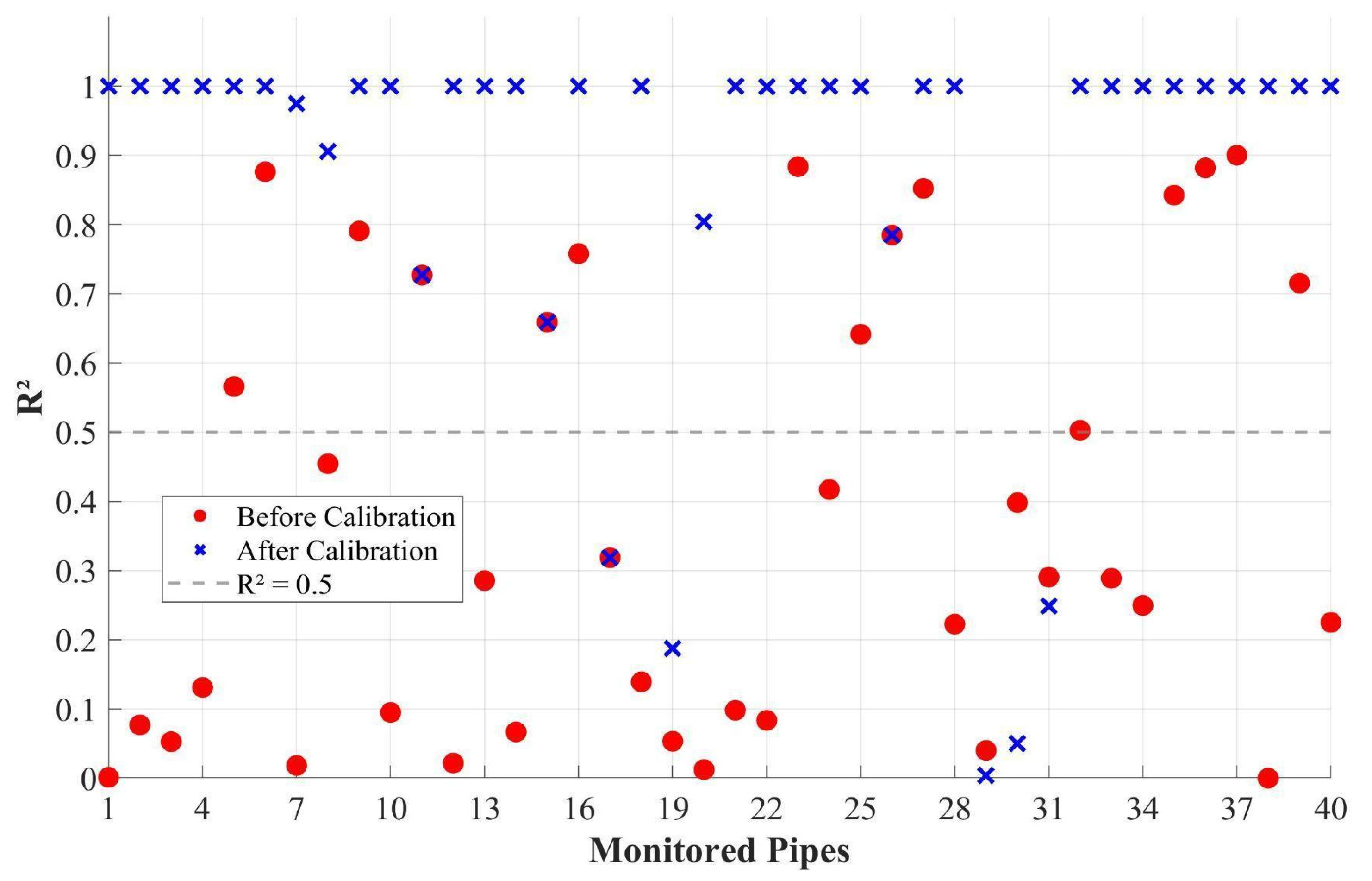
3. Results
4. Discussion
5. Conclusions
Author Contributions
Funding
Data Availability Statement
Acknowledgments
Conflicts of Interest
References
- Dighade, R.R.; Kadu, M.S.; Pande, A.M. Challenges in water loss management of water distribution systems in developing countries. Int. J. Innov. Res. Sci. Eng. Technol. 2014, 3, 13838–13846. [Google Scholar]
- Kizilöz, B. Prediction model for the leakage rate in a water distribution system. Water Sup. 2021, 21, 4481–4492. [Google Scholar] [CrossRef]
- Greve, P.; Kahil, T.; Mochizuki, J.; Schinko, T.; Satoh, Y.; Burek, P.; Fischer, G.; Tramberend, S.; Burtscher, R.; Langan, S.; et al. Global assessment of water challenges under uncertainty in water scarcity projections. Nat. Sustain. 2018, 1, 486–494. [Google Scholar] [CrossRef]
- Rustam, F.; Ishaq, A.; Kokab, S.T.; de la Torre Diez, I.; Mazón, J.L.V.; Rodríguez, C.L.; Ashraf, I. An Artificial Neural Network Model for Water Quality and Water Consumption Prediction. Water 2024, 21, 3359. [Google Scholar] [CrossRef]
- Campos, J.N.B.; Lima Neto, I.E.; Studart, T.M.C.; Nascimento, L.S.V. Trade-off between reservoir yield and evaporation losses as a function of lake morphology in semi-arid Brazil. Ann. Braz. Acad. Sci. 2016, 88, 1113–1125. [Google Scholar] [CrossRef]
- Pereira, B.; Uchôa, J.G.; Freitas, G.; Meira Neto, A.A.; Anache, J.; Wendland, E.C.; Mendiondo, E.M.; Medeiros, P. Hydrological Heritage: A Historical Exploration of Human-Water Dynamics in Northeast Brazil. Hydrol. Sci. J. 2024, 16. [Google Scholar] [CrossRef]
- Meirelles, G.; Manzi, D.; Brentan, B.; Goulart, T.; Luvizotto, E., Jr. Calibration model for water distribution network using pressure heads estimated by artificial neural networks. Water Resour. Manag. 2017, 31, 4339–4351. [Google Scholar] [CrossRef]
- Zhao, Q.; Wu, W.; Simpson, A.R.; Willis, A. Simpler Is Better—Calibration of Pipe Roughness in Water Distribution Systems. Water 2022, 14, 3276. [Google Scholar] [CrossRef]
- Savic, D.A.; Kapelan, Z.S.; Jonkergouw, P.M.R. Quo vadis water distribution model calibration? Urban Water J. 2009, 6, 3–22. [Google Scholar] [CrossRef]
- Ferreira, B.; Antunes, A.; Carriço, N.; Covas, D. Multi-objective optimization of pressure head sensor location for burst detection and network calibration. Comput. Chem. Eng. 2022, 162, 107826. [Google Scholar] [CrossRef]
- Maskit, M.; Ostfeld, A. Multi-Objective Operation-Leakage Optimization and Calibration of Water Distribution Systems. Water 2021, 13, 1606. [Google Scholar] [CrossRef]
- Zanfei, A.; Menapace, A.; Brentan, B.; Sitzenfrei, R.; Herrera, M. Shall we always use hydraulic models? A graph neural network metamodel for water system calibration and uncertainty assessment. Water Res. 2023, 242, 120264. [Google Scholar] [CrossRef] [PubMed]
- Nicolini, M.; Giacomello, C.; Deb, K. Calibration and Optimal Leakage Management for a Real Water Distribution Network. J. Water Resour. Plann. Manag. 2011, 137, 134–142. [Google Scholar] [CrossRef]
- Salvino, M.M.; Carvalho, P.S.O.; Gomes, H.P. Calibração multivariada de redes de abastecimento de água via algoritmo genético multiobjetivo. Eng. Sanit. Ambient. 2015, 20, 503–512. [Google Scholar] [CrossRef]
- Romero-Ben, L.; Alvez, D.; Blesa, J.; Cembrano, G.; Puig, V.; Duviella, E. Leak detection and localization in water distribution networks: Review and perspective. Annu. Rev. Control 2023, 55, 392–419. [Google Scholar] [CrossRef]
- Osorio, D.A.J.; Lima, G.M.; Brentan, B.M. Hydraulic and economic analysis for rehabilitation of water distribution networks using pipes cleaning and replacement and leakage fixing. Braz. J. Water Resour. 2023, 28, e6. [Google Scholar] [CrossRef]
- Garzón, A.; Kapelan, Z.; Langeveld, J.; Taormina, R. Machine Learning-Based Surrogate Modeling for Urban Water Networks: Review and Future Research Directions. Water Resour. Res. 2022, 58, e2021WR031808. [Google Scholar] [CrossRef]
- Moasheri, R.; Ghazizadeh, M.J.; Tashayoei, M. Leakage detection in water networks by a calibration method. Flow Meas. Instrum. 2021, 80, 101995. [Google Scholar] [CrossRef]
- Farghadan, A.; Zamani, M.S.; Ghazizadeh, M.J. A fault-injection-based approach to leak localization in water distribution networks using an ensemble model of Bayesian classifiers. J. Process Control 2023, 132, 103110. [Google Scholar] [CrossRef]
- Chu, S.; Zhang, T.; Zhou, X.; Yu, T.; Shao, Y. An Efficient Approach for Nodal Water Demand Estimation in Large-scale Water Distribution Systems. Water Resour. Manag. 2022, 36, 491–505. [Google Scholar] [CrossRef]
- Ostfeld, A.; Salomons, E.; Ormsbee, L.; Uber, J.G.; Bros, C.M.; Kalungi, P.; Burd, R.; Zazula-Coetzee, B.; Belrain, T.; Kang, D.; et al. Battle of the Water Calibration Networks. J. Water Resour. Plann. Manag. 2012, 138, 523–532. [Google Scholar] [CrossRef]
- Zhang, Q.; Zheng, F.; Duan, H.-F.; Jia, Y.; Zhang, T.; Guo, X. Efficient Numerical Approach for Simultaneous Calibration of Pipe Roughness Coefficients and Nodal Demands for Water Distribution Systems. J. Water Resour. Plann. Manag. 2018, 144, 04018063. [Google Scholar] [CrossRef]
- Chu, S.; Zhang, T.; Shao, Y.; Yu, T.; Yao, H. Numerical approach for water distribution system model calibration through incorporation of multiple stochastic prior distributions. Sci. Total Environ. 2020, 708, 134565. [Google Scholar] [CrossRef] [PubMed]
- Zhang, Q.; Yang, J.; Zhang, W.; Kumar, M.; Liu, J.; Liu, J.; Li, X. Deep fuzzy mapping nonparametric model for real-time demand estimation in water distribution systems: A new perspective. Water Res. 2023, 241, 120145. [Google Scholar] [CrossRef] [PubMed]
- Nicklow, J.; Reed, P.; Savic, D.; Dessalegne, T.; Harrell, L.; Chan-Hilton, A.; Karamouz, M.; Minsker, B.; Ostfeld, A.; Singh, A.; et al. State of the Art for Genetic Algorithms and Beyond in Water Resources Planning and Management. J. Water Resour. Plann. Manag. 2010, 136, 412–432. [Google Scholar] [CrossRef]
- Zhang, L.; Jiang, H.; Cao, H.; Cheng, R.; Zhang, J.; Du, F.; Xie, K. Water Supply Pipeline Failure Evaluation Model Based on Particle Swarm Optimization Neural Network. Water 2024, 16, 3248. [Google Scholar] [CrossRef]
- Minaee, R.P.; Afsharnia, M.; Moghaddam, A.; Ebrahimi, A.A.; Askarishahi, M.; Mokhtari, M. Calibration of water quality model for distribution networks using genetic algorithm, particle swarm optimization, and hybrid methods. MethodsX 2019, 6, 540–548. [Google Scholar] [CrossRef]
- Jahandideh-Tehrani, M.; Bozorg-Haddad, O.; Loáiciga, H.A. Application of particle swarm optimization to water management: An introduction and overview. Environ. Monit. Assess. 2020, 192, 281. [Google Scholar] [CrossRef]
- Souza Filho, F.A. CEARÁ 2050: Diagnóstico dos Recursos Hídricos; Ceará: Fortaleza, Brazil, 2018. [Google Scholar]
- Walker, D.W.; Oliveira, J.L.; Cavalcante, L.; Kchouk, S.; Ribeiro Neto, G.; Melsen, L.A.; Fernandes, F.B.P.; Mitroi, V.; Gondim, R.S.; Martins, E.S.P.R.; et al. It’s not all about drought: What “drought impacts” monitoring can reveal. Int. J. Disaster Risk Reduct. 2024, 103, 104338. [Google Scholar] [CrossRef]
- Silva, S.M.O.; Souza Filho, F.A.; Cid, D.A.C.; Aquino, S.H.S.; Xavier, L.C.P. Proposta de gestão integrada das águas urbanas como estratégia de promoção da segurança hídrica: O caso de Fortaleza. Eng. Sanit. Ambient. 2019, 24, 239–250. [Google Scholar] [CrossRef]
- Uchôa, J.G.S.M.; Almeida, P.P.; Marques, L.A.; Pereira, S.P.; Silva, S.M.O.; Lima Neto, I.E. Análise do impacto da usina de dessalinização no macrossistema de abastecimento de água da região metropolitana de Fortaleza—CE. In Proceedings of the I Simpósio Nacional de Mecânica dos Fluidos e Hidráulica, Ouro Preto, MG, Brazil, 22–24 August 2022. [Google Scholar]
- CAGECE—Companhia de Água e Esgoto do Ceará. Planta de Dessalinização de Água Marinha. Available online: https://www.cagece.com.br/wp-content/uploads/PDF/EditaisContratacoes/PPP/Documentos-Relatorio/Relatorio_desempenho_de_projeto_PPP-Desal-1_assdpr.pdf (accessed on 7 January 2025).
- Rathi, S.; Gupta, R.; Labhasetwar, P.; Nagarnaik, P. Challenges in calibration of water distribution network: A case study of Ramnagar elevated service reservoir command area in Nagpur City, India. Water Sup. 2020, 20, 1294–1312. [Google Scholar] [CrossRef]
- Leinæs, A.; Simukonda, K.; Farmani, R. Calibration of intermittent water supply systems hydraulic models under data scarcity. Water Sup. 2024, 24, 1626–1644. [Google Scholar] [CrossRef]
- Hossain, S.; Hewa, G.A.; Chow, C.W.K.; Cook, D. Modelling and Incorporating the Variable Demand Patterns to the Calibration of Water Distribution System Hydraulic Model. Water 2021, 13, 2890. [Google Scholar] [CrossRef]
- Kennedy, J.; Eberhart, R. Particle swarm optimization. In Proceedings of the ICNN’95-International Conference on Neural Networks, Perth, WA, USA, 27 November–1 December 1995; Volume 4, pp. 1942–1948. [Google Scholar] [CrossRef]
- Anchieta, T.F.F.; Meirelles, G.; Brentan, B.M. Optimal district metered areas design of water distribution systems: A comparative analysis among hybrid algorithms. J. Water Process Eng. 2024, 63, 105472. [Google Scholar] [CrossRef]
- Rahman, N.A.; Muhammad, N.S.; Abdullah, J.; Mohtar, W.H.M.W. Model performance indicator of aging pipes in a domestic water supply distribution network. Water 2019, 11, 2378. [Google Scholar] [CrossRef]
- Ghimire, A.B.; Magar, B.A.; Parajuli, U.; Shin, S. Impacts of Missing Data Imputation on Resilience Evaluation for Water Distribution System. Urban Sci. 2024, 8, 177. [Google Scholar] [CrossRef]
- Farmani, R.; Savic, D.A.; Walters, G.A. Evolutionary multi-objective optimization in water distribution network design. Eng. Optim. 2005, 37, 167–183. [Google Scholar] [CrossRef]
- Housh, M.; Jamal, A. Utilizing Matrix Completion for Simulation and Optimization of Water Distribution Networks. Water Resour. Manag. 2022, 36, 1–20. [Google Scholar] [CrossRef]
- Water Research Centre. Network Analysis—A Code of Practice; WRc: Swindon, UK, 1989. [Google Scholar]
- Kapelan, Z.S.; Savic, D.A.; Walters, G.A. Calibration of Water Distribution Hydraulic Models Using a Bayesian-Type Procedure. J. Hydraul. Eng. 2007, 133, 927–936. [Google Scholar] [CrossRef]
- Moriasi, D.N.; Arnold, J.G.; Van Liew, M.W.; Bingner, R.L.; Harmel, R.D.; Veith, T.L. Model Evaluation Guidelines for Systematic Quantification of Accuracy in Watershed Simulations. ASABE 2007, 50, 885–900. [Google Scholar] [CrossRef]
- Zarei, N.; Azari, A.; Heidari, M.M. Improvement of the performance of NSGA-II and MOPSO algorithms in multi-objective optimization of urban water distribution networks based on modification of decision space. Appl. Water Sci. 2022, 12, 133. [Google Scholar] [CrossRef]
- Sabbaghpour, S.; Naghashzadehgan, M.; Javaherdeh, K.; Bozorg-Haddad, O. HBMO algorithm for calibrating water distribution network of Langarud city. Water Sci. Technol. 2012, 65, 1564–1569. [Google Scholar] [CrossRef] [PubMed]
- Jadhao, R.D.; Gupta, R. Calibration of water distribution network of the Ramnagar zone in Nagpur City using online pressure head and flow rate data. Appl. Water Sci. 2018, 8, 29. [Google Scholar] [CrossRef]
- Zanfei, A.; Menapace, A.; Santopietro, S.; Righetti, M. Calibration Procedure for Water Distribution Systems: Comparison among Hydraulic Models. Water 2020, 12, 1421. [Google Scholar] [CrossRef]
- Ballarin, A.S.; Sousa Mota Uchôa, J.G.; Santos, M.S.; Almagro, A.; Miranda, I.P.; Silva, P.G.; Silva, G.J.; Gomes Júnior, M.N.; Wendland, E.; Oliveira, P.T. Brazilian water security threatened by climate change and human behavior. Water Resour. Res. 2023, 59, e2023WR034914. [Google Scholar] [CrossRef]


| Diameter | Number | Extension (km) |
|---|---|---|
| ≤200 mm | 61 | 1.73 |
| 200–400 mm | 43 | 9.94 |
| 400–600 mm | 105 | 46.19 |
| 600–1000 mm | 107 | 60.06 |
| ≥1000 mm | 77 | 84.67 |
| Total | 393 | 202.59 |
| Indicators | Equations |
|---|---|
| Mean Absolute Error | |
| Average Relative Hourly Error (%) | |
| Nash–Sutcliffe Efficiency Coefficient | |
| Coefficient of Determination | |
| Percentual Bias (%) |
| MAE | ARHE | NSE | R2 | PBIAS | |
|---|---|---|---|---|---|
| Before Calibration | 7.10 m | 31.13% | 0.597 | 0.623 | 2.64% |
| After Calibration | 3.53 m | 12.96% | 0.873 | 0.879 | 3.38% |
| MAE | ARHE | NSE | R2 | PBIAS | |
|---|---|---|---|---|---|
| Before Calibration | 43.7 L/s | 320.79% | 0.754 | 0.780 | 11.80% |
| After Calibration | 16.3 L/s | 13.09% | 0.965 | 0.965 | 1.06% |
Disclaimer/Publisher’s Note: The statements, opinions and data contained in all publications are solely those of the individual author(s) and contributor(s) and not of MDPI and/or the editor(s). MDPI and/or the editor(s) disclaim responsibility for any injury to people or property resulting from any ideas, methods, instructions or products referred to in the content. |
© 2025 by the authors. Licensee MDPI, Basel, Switzerland. This article is an open access article distributed under the terms and conditions of the Creative Commons Attribution (CC BY) license (https://creativecommons.org/licenses/by/4.0/).
Share and Cite
Rocha, J.S.; Uchôa, J.G.S.M.; Brentan, B.M.; Neto, I.E.L. Key Calibration Strategies for Mitigation of Water Scarcity in the Water Supply Macrosystem of a Brazilian City. Water 2025, 17, 883. https://doi.org/10.3390/w17060883
Rocha JS, Uchôa JGSM, Brentan BM, Neto IEL. Key Calibration Strategies for Mitigation of Water Scarcity in the Water Supply Macrosystem of a Brazilian City. Water. 2025; 17(6):883. https://doi.org/10.3390/w17060883
Chicago/Turabian StyleRocha, Jefferson S., José Gescilam S. M. Uchôa, Bruno M. Brentan, and Iran E. Lima Neto. 2025. "Key Calibration Strategies for Mitigation of Water Scarcity in the Water Supply Macrosystem of a Brazilian City" Water 17, no. 6: 883. https://doi.org/10.3390/w17060883
APA StyleRocha, J. S., Uchôa, J. G. S. M., Brentan, B. M., & Neto, I. E. L. (2025). Key Calibration Strategies for Mitigation of Water Scarcity in the Water Supply Macrosystem of a Brazilian City. Water, 17(6), 883. https://doi.org/10.3390/w17060883