Shallow Subsurface Soil Moisture Estimation in Coal Mining Area Using GPR Signal Features and BP Neural Network

Abstract

Coal mining disrupts soil structure and causes water loss, thereby affecting the ecological environment of mining areas. Rapid, accurate, and non-destructive detection of surface soil moisture is crucial for advancing ecological restoration in these regions. This study focuses on the mined and unmined areas of the Yushuquan coal mine, located on the southern slope of the Tianshan Mountains in Xinjiang, China. The soil volumetric water content (SVWC) was measured using time-domain reflectometry (TDR), while the shallow subsurface soil was investigated using ground-penetrating radar (GPR). Various features were extracted from GPR signals in both the time- and frequency-domains, and their relationships with SVWC were analyzed. Multiple features were selected and optimized to determine the optimal feature combination for building a multi-feature backpropagation neural network model for soil volumetric water content prediction (Muti-BP-SVWC). The performance of this model was compared with two single-feature-based methods for SVWC prediction: the average envelope amplitude (AEA) method and the frequency shift method. The application results of the Muti-BP-SVWC model in different regions demonstrated significant improvements in accuracy and stability compared to the AEA method and the frequency shift method. In the mined area validation set, the model achieved an determination coefficient (R²) of 0.77 and the root mean square error (RMSE) of 0.0091 cm³/cm³, while in the unmined area validation set, the R² of 0.84 and an RMSE of 0.0059 cm³/cm³. These results indicate that incorporating multiple features into the BP neural network can better capture the complex relationship between GPR signals and SVWC. This approach effectively inverts the shallow subsurface soil moisture in mining areas and provides valuable guidance for ecological restoration in these regions.

1. Introduction

Most coal mining areas in western China are situated in semi-arid regions undergoing desertification, where the ecological environment is extremely fragile. Coal mining activities result in ground subsidence and surface cracks, altering the soil’s porosity and bulk density, along with its other physical and chemical properties. These changes affect the distribution of soil moisture, leading to plant wilting and exacerbating environmental degradation [1]. Therefore, rapid and accurate measurement of soil moisture content is of great significance for environmental management and ecological restoration in mining areas [2,3]. Traditional methods for measuring soil volumetric water content (SVWC), such as the oven-drying method, time-domain reflectometry (TDR) method, and neutron probe method, although highly accurate, typically rely on point measurements. These methods are time-consuming, labor-intensive, and destructive, making large-scale, rapid detection challenging [4,5,6,7,8]. While remote sensing technology can cover extensive areas, it is constrained by limited detection depths and relatively low spatial resolution, restricting its effectiveness in meeting the needs of ecological restoration [9,10].

Ground-penetrating radar (GPR) is a non-invasive detection technique that employs high-frequency electromagnetic pulses to penetrate underground media and receive signals reflected from various depths. By analyzing the waveform, amplitude, velocity, and other characteristics of these echo signals, researchers can infer the spatial position, structure, moisture content, and other physical properties of the subsurface materials. GPR provides continuous data acquisition, high efficiency and high resolution, making it widely applicable in soil moisture detection studies [11,12].

Currently, most researchers utilize methods based on the relationship between wave velocity and dielectric permittivity, including reflected waves, ground waves, and borehole radar techniques, to estimate the dielectric permittivity of the medium by measuring the propagation speed of electromagnetic waves. The dielectric permittivity is then converted into SVWC using the TOPP equation [13,14,15,16,17,18]. However, the accuracy of these methods is often limited by the difficulties in obtaining precise wave velocities. For instance, the reflected wave method necessitates a clear underground reflective interface, and determining the depth of this interface typically requires dense drilling [15], while the ground wave method determines wave velocity by analyzing the slope of the two-way travel time of the ground waves relative to the antenna separation. Although it does not rely on an underground reflective interface, this method is easily affected by noise, such as air waves and reflected waves, making the separation and identification of ground waves challenging [19].

As research progressed, scholars increasingly recognized the challenges in obtaining accurate wave velocities. Consequently, some researchers shifted their focus to analyzing GPR signal features. Numerous theoretical derivations, numerical simulations, and laboratory experiments have demonstrated that the shape, amplitude, and onset time of the early time signal from GPR are closely related to the soil dielectric permittivity. The average envelope amplitude (AEA) method quantifies the relationship between the amplitude envelope of the early time signal and the dielectric permittivity to estimate SVWC [20,21,22,23,24]. Compared to traditional velocity–dielectric permittivity methods, this approach does not rely on a reflective interface and remains applicable even under conditions with strong electromagnetic wave attenuation or mixed ground and air waves. However, the accuracy of this time-domain method for estimating soil moisture content is influenced by the correlation model and the TOPP equation, which can introduce secondary errors [25]. The frequency shift method employs fast Fourier transform (FFT) to convert GPR signals from the time-domain to the frequency-domain. Based on Rayleigh scattering theory, it establishes a relationship between peak frequency (PF) and SVWC by utilizing the pattern of the spectrum shifting toward lower frequencies as soil moisture increases. This method does not require calculating the soil dielectric permittivity or performing complex calibration processes, allowing for rapid SVWC estimation [26,27,28]. Subsequently, more researchers have explored various spectral analysis techniques to investigate the relationships between frequency-domain features of GPR signals and the physical properties of geotechnical materials [29,30,31,32,33,34,35].

Despite significant progress in using GPR signal features to estimate SVWC, most studies use linear regression models to establish the relationship between GPR signal features and SVWC. Such an approach is insufficient for capturing the complex nonlinear relationships between GPR signals and SVWC [36,37]. In recent years, machine learning techniques have rapidly developed across various fields, demonstrating remarkable capability and accuracy in capturing the internal relationships between data variables within datasets. Some researchers have started applying machine learning methods to capture the nonlinear relationship between radar signal features and SVWC. Li Z et al. used convolutional neural networks to establish a relationship between GPR data and SVWC [38]. LI X et al. proposed a deep learning-based GPR data inversion model, PyViTENet, which integrates pyramid convolution and vision transformer for feature extraction, achieving high-precision dielectric permittivity inversion of underground tree roots and their surrounding soil [39]. Zhang X et al. proposed a GPR-CUNet model, which combines a CNN and BiLSTM for spatiotemporal feature fusion and uses a dual U-Net structure to achieve the mutual transformation between the permittivity distribution and GPR B-Scan data [40]. These models are capable of effectively handling complex nonlinear problems, improving the prediction accuracy of SVWC.

However, despite these advancements, most studies still focus on analyzing individual or specific types of features, without conducting a comprehensive analysis of the GPR signal. And many studies are carried out under laboratory conditions, where physical parameters are precisely controlled, feature analysis methods often achieve high prediction accuracy. Nevertheless, the applicability of some models in field environments remains limited, as factors such as soil heterogeneity, geological complexity, and signal noise lead to reduced accuracy in SVWC prediction [41]. Moreover, in research related to the impact of coal mining on soil moisture, most studies only focus on a single condition, either the mined or unmined area.

In this context, this study comprehensively analyzed the relationship between both time-domain and frequency-domain features of GPR signals and SVWC. We employ a backpropagation (BP) neural network to integrate multiple GPR signal features to develop an SVWC prediction (Muti-BP-SVWC) model in mined and unmined areas. The proposed approach aims to improve the accuracy and reliability of soil moisture predictions, providing technical support for rapid soil moisture detection and ecological restoration in mining areas.

2. Materials and Methods

2.1. Study Area

The Yushuquan coal mine is located at the southern foothills of the Tianshan Mountains in Xinjiang Province, within the Jiestdlik Syncline on the northern edge of the Tarim Basin. The overall terrain exhibits a basin characteristic, with higher elevations in the north and south and a lower central region, resulting in a relative difference in elevation ranging from 10 to 50 m. The surface within the coal mine area is dominated by exposed bedrock, sparse vegetation, and several small north–south oriented gullies. The bedrock features steep cliffs, unusual rock formations, and significant wind erosion, giving rise to a “Yadan” landform. The climate is classified as a northern warm temperate continental arid, with limited precipitation and considerable annual and diurnal temperature variations. The annual average temperature is 11.4 °C, with average annual precipitation of 262 mm and evaporation reaching 2860 mm. The Yushuquan coal mine employs a slope mining method and longwall mining techniques, extracting coal seams above the +1783 level with seam thicknesses ranging from 4.20 m to 4.30 m.

2.2. Data Acquisition

In a working face of the Yushuquan coal mine, the study area (Figure 1a) was divided into the mined and unmined zones (Figure 1b). Based on geological condition analysis, GPR survey lines and TDR measurement points were laid out in both regions. In the mined area, four inlines were laid in a north–south direction, each 280 m long with a 60-m spacing between lines, and one east–west crossline, 200 m long, with 17 TDR measurement points (Figure 1c). In the unmined area, three inlines were laid in a north–south direction, each 280 m long with a 40 m spacing between lines, and one east–west crossline, 100 m long, with 14 TDR measurement points (Figure 1d).

The equipment used was the GR series GPR developed by the China University of Mining and Technology, Beijing (CUMTB), with a central antenna frequency of 300 MHz, 1024 sampling points, and a 50 ns sampling time window. Position marking was performed at 10 m intervals. The common offset method was used for rapid measurement of the survey area. Raw GPR data are subject to interference across various frequencies, along with low-frequency drift, leading to baseline instability that can obscure reflection signals. To address this, a one-dimensional band-pass filter was applied to attenuate unwanted components and improve the signal-to-noise ratio. The filter parameters were selected based on the GPR antenna’s central frequency, with a lower cutoff of 140 MHz and an upper cutoff of 900 MHz. Figure 2 shows a GPR profile extracted from a survey line, with the time window of the early time signals approximately ranging from 0 ns to 14 ns. Additionally, SVWC in the 0–50 cm depth range was measured at predefined points by excavating a 0–50 cm soil profile. The five probes of the ECH₂O-5TM soil moisture sensor, developed by Meter Group, USA (Pullman, WA, USA), were evenly inserted at different depths within the 0–50 cm range, and the average soil moisture content was then calculated.

2.3. Principles for Time-Domain Feature-Based SVWC Estimation

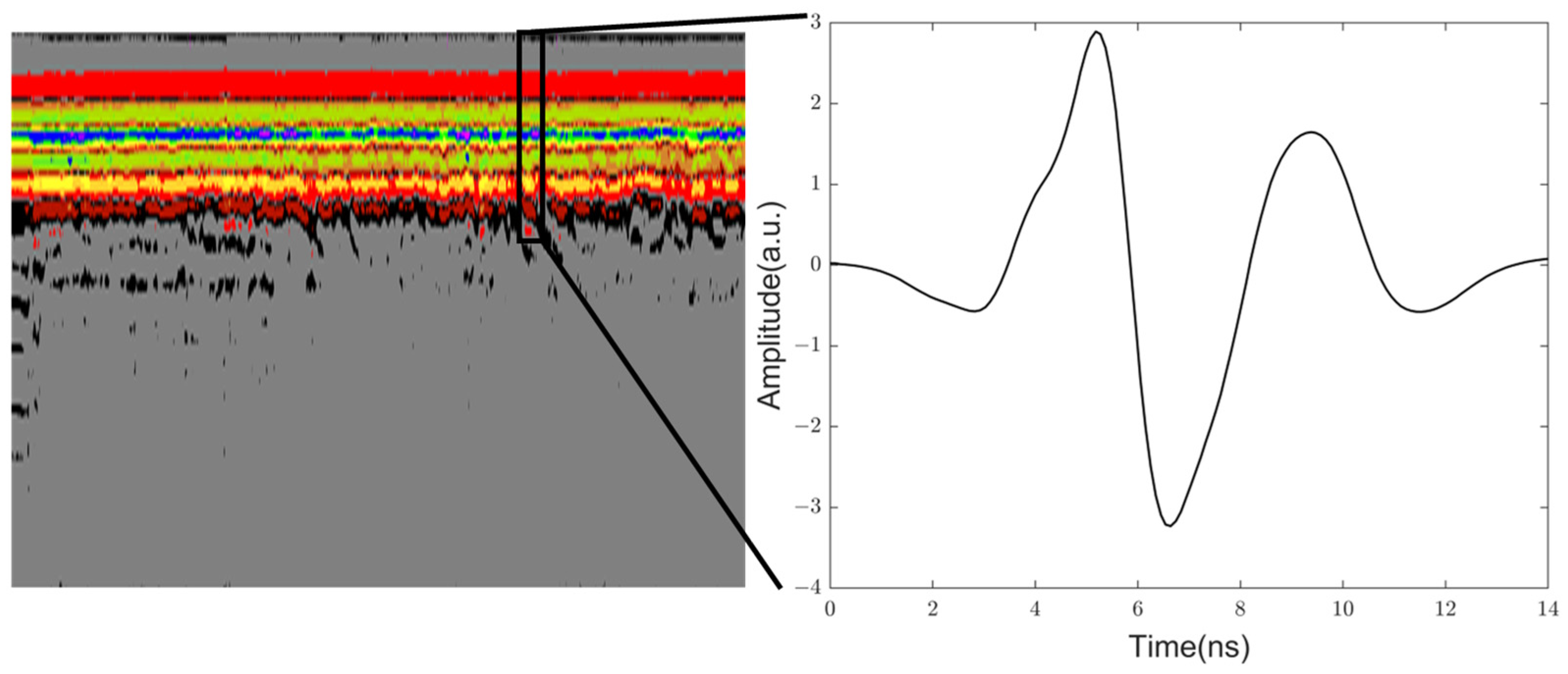
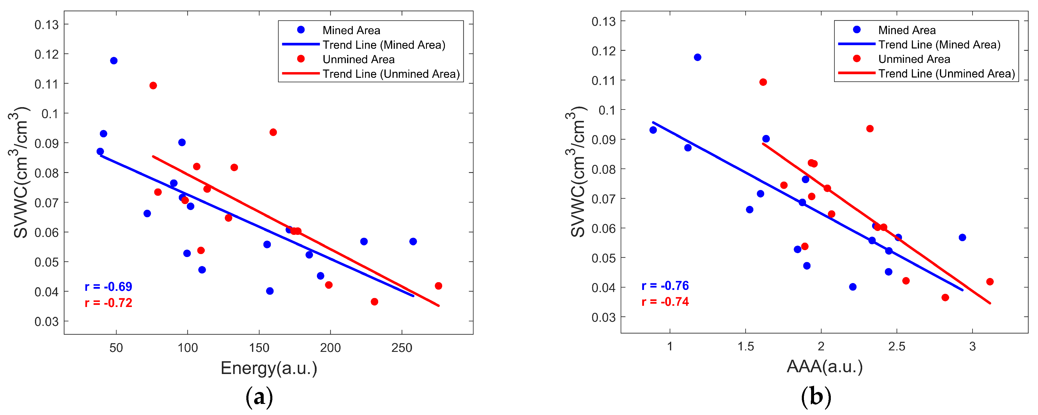
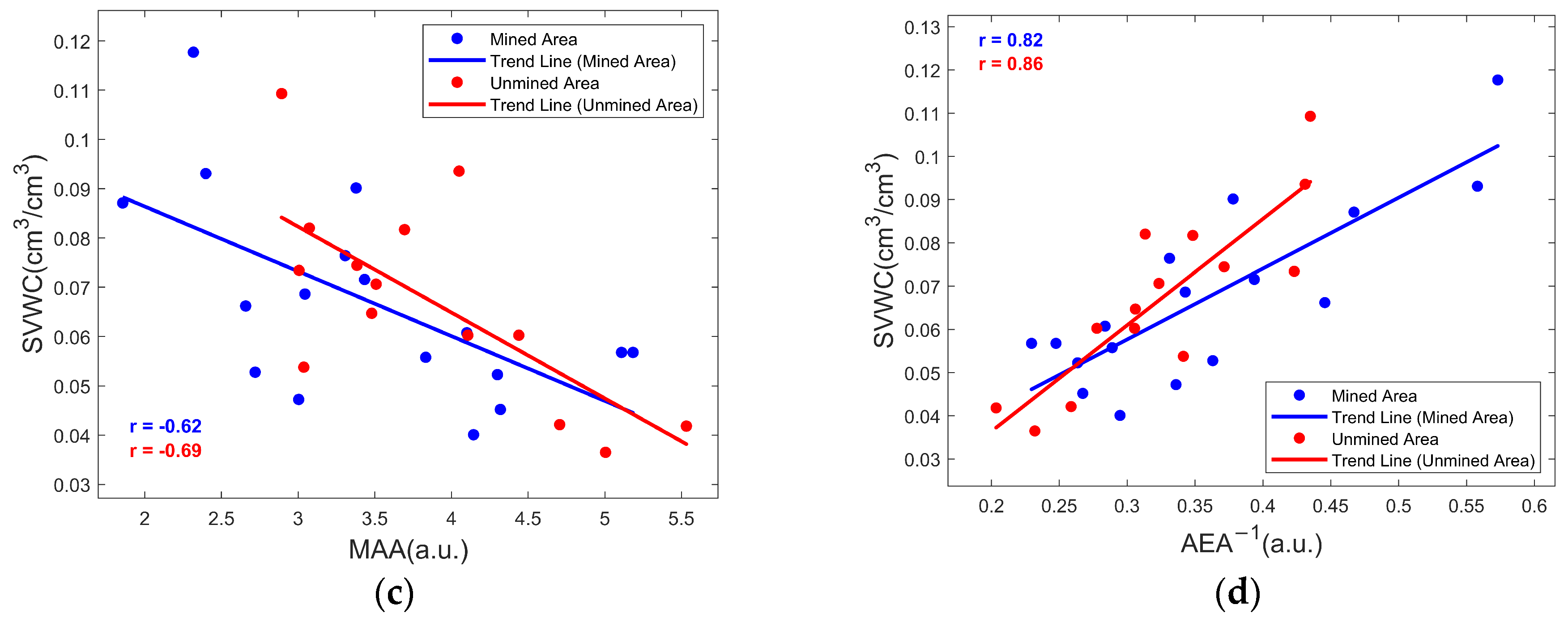
2.3.1. Raw Time-Domain Features

In the common-offset detection method, the antenna separation of the GPR is relatively short, and when this distance is smaller than the wavelength of the electromagnetic waves, the early time signals become a mixture of airwaves and ground waves. The relationships between airwaves, ground waves, and dielectric permittivity are given by the following [22]:

$$A_{air-wave}={\displaystyle \frac{\sqrt{{\epsilon }_0{\mu }_0}}{2\pi {\epsilon }_0\left({\epsilon }_r-1\right)S^2}}$$

(1)

$$A_{ground-wave}=-A_{ground-wave}^0\exp \left(-\left({\displaystyle \frac{1}{2}}\right){\displaystyle \frac{\sqrt{{\mu }_0}}{{\epsilon }_0{\epsilon }_r}}\sigma S\right)$$

(2)

$$A_{ground-wave}^0={\displaystyle \frac{\sqrt{{\epsilon }_r{\mu }_0}}{2\pi {\epsilon }_0\left({\epsilon }_r-1\right)S^2}}$$

(3)

where $A_{air-wave}$ and $A_{ground-wave}$ represent the amplitudes of the airwave and ground wave, while $A_{ground-wave}^0$ is the amplitude of the ground wave in a vacuum. ${\epsilon }_0$ and ${\mu }_0$ are the permittivity and permeability of the free space, respectively, and ${\epsilon }_r$ is the relative permittivity of the medium. $\sigma$ is the conductivity, and $S$ is the antenna separation. The exponential term in Equation (2) indicates the rapid attenuation of ground waves, and both Equations (2) and (3) show that $A_{air-wave}$ and $A_{ground-wave}$ are inversely proportional to the dielectric permittivity. Since the ${\epsilon }_r$ of air is 1, that of solid particles is approximately 3 to 6, and that of water is 81, the SVWC becomes the key factor determining soil dielectric permittivity. Therefore, by measuring the amplitude variation in the early signal, the soil moisture content can be inferred. Figure 3 shows the amplitude of the single-trace GPR early time signals collected under different SVWC conditions in the unmined area. It can be observed that the signal amplitude increases as the soil moisture content decreases.

To quantitatively describe the changes in amplitude, three original time-domain features are introduced: energy, absolute amplitude average (AAA), and maximum absolute amplitude (MAA), which are expressed as follows:

$$Energy={{\displaystyle {\int }_{t1}^{t2}A\left(t\right)}}^{2}dt$$

(4)

$$AAA={\displaystyle \frac{1}{t_2-t_1}}{\displaystyle {\int }_{t_1}^{t_2}\left|A(t)\right|}dt$$

(5)

$$MAA=\underset{t\in \left[t_1,t_2\right]}{\max }\left|A\left(t\right)\right|$$

(6)

where $A(t)$ represents the amplitude value at a given time, with $t_1$ and $t_2$ defining the limits of the time window.

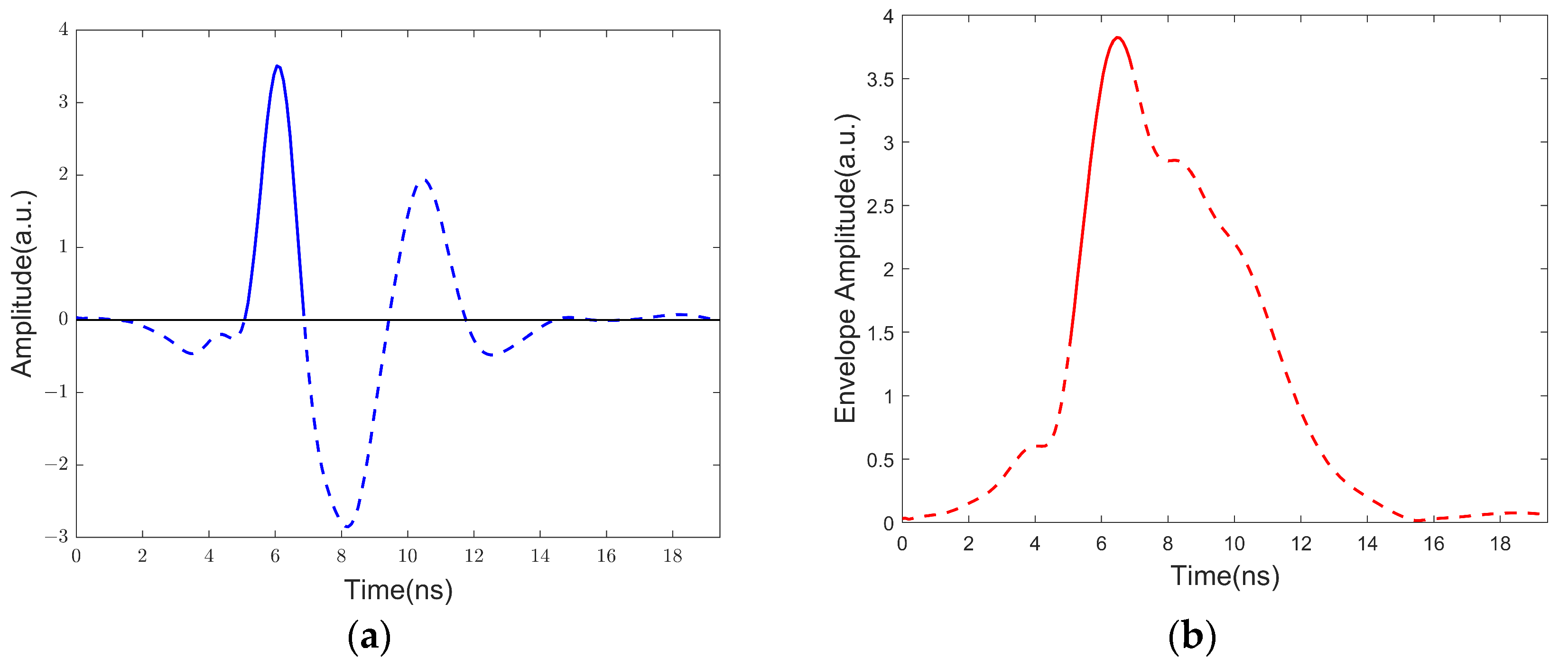
2.3.2. Average Envelope Amplitude

The raw time-domain signal contains complex waveform and phase information, while the envelope amplitude simplifies it into a real number sequence, making the variation in signal strength over time more intuitive and easier to analyze. To extract the amplitude envelope, the GPR signal, which is considered a continuous function of time, $x(t)$, is processed using a Hilbert transform [41]:

$$H\left(x(t)\right)={\displaystyle \frac{1}{\pi }}{\displaystyle {\int }_{-\infty }^{+\infty }\frac{x\left(\tau \right)}{t-\tau }}d\tau$$

(7)

The original signal, $x(t)$, is taken as the real part, and the imaginary part, $\widehat{x}(t)$, after the Hilbert transform is combined to form the analytic signal, $z(t)$, as shown in Equation (8):

$$z(t)=x(t)+j\widehat{x}(t)$$

(8)

The envelope amplitude can be obtained by calculating the modulus of $z(t)$:

$$A(t)=\left|z(t)\right|=\sqrt{x{(t)}^2+\widehat{x}{(t)}^2}$$

(9)

Research shows that the AEA⁻¹ of the first positive half-cycle of the early time signal has the strongest correlation with dielectric permittivity. Therefore, in this study, the envelope amplitude of the first positive half-cycle of the GPR signal was discretely integrated, divided by the unit length of integration, and its reciprocal was taken to obtain AEA⁻¹ [22,24]. Figure 4 illustrates the conversion of a randomly selected single-trace GPR signal into its envelope amplitude.

2.4. Principles for Frequency-Domain Feature-Based SVWC Estimation

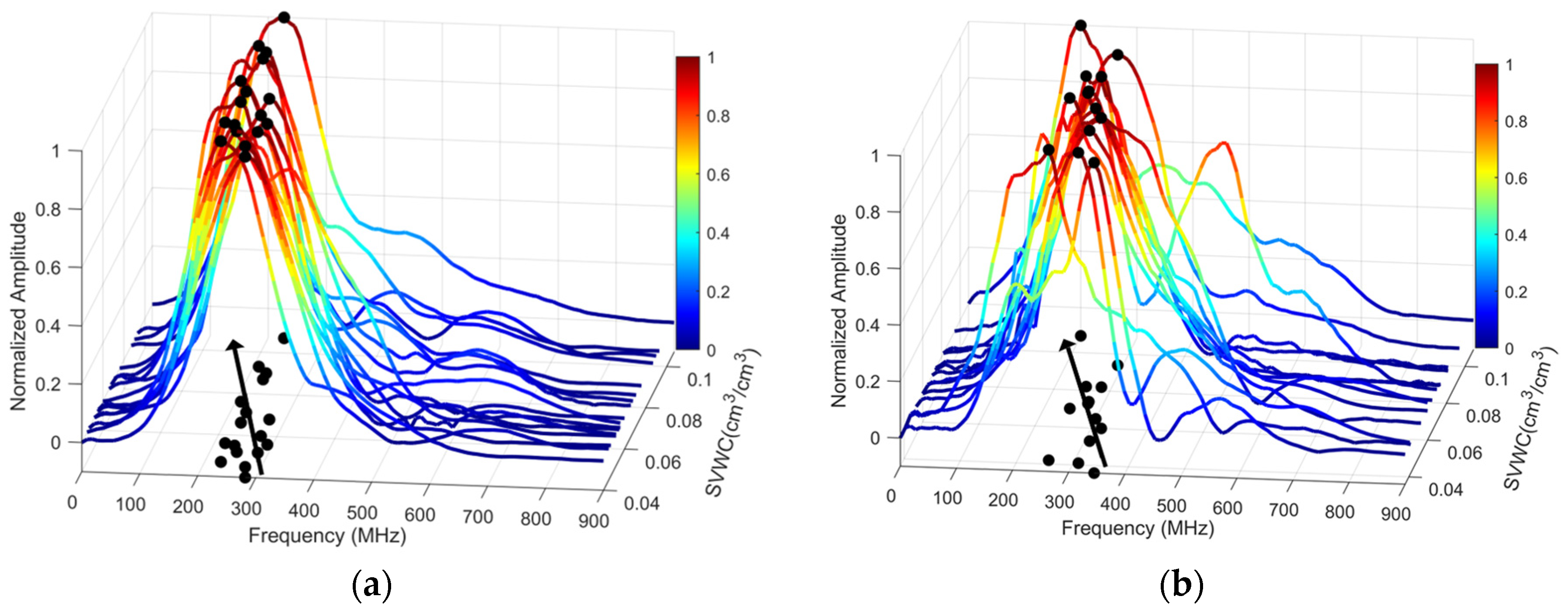
2.4.1. Rayleigh Scattering

Rayleigh scattering refers to the phenomenon where electromagnetic waves are scattered by particles much smaller than the wavelength. The scattering intensity is given by [42]:

$$I=I_0\left({\displaystyle \frac{1+{\cos }^2\theta }{2R^2}}\right){\left({\displaystyle \frac{2\pi }{\lambda }}\right)}^4{\left({\displaystyle \frac{n^2-1}{n^2+2}}\right)}^2\left({\displaystyle \frac{d}{2}}\right)$$

(10)

where $I$ is the intensity of the scattered wave, $I_0$ is the intensity of the incident wave, $n$ is the refractive index of the particle, $d$ is the diameter of the particle, $\lambda$ is the wavelength of the electromagnetic wave, $\theta$ is the scattering angle, and $R$ is the distance from the observer to the particle. From the equation, it can be seen that the intensity of the electromagnetic wave scattering is proportional to the fourth power of the frequency, meaning that higher frequencies scatter more strongly. Additionally, a larger refractive index results in stronger scattering. Assuming a non-magnetic medium, linear polarization, no free charges, and zero current density, the refractive index can be derived from Maxwell’s equations as follows [26,27]:

$$n=\sqrt{{\epsilon }_r{\mu }_r}$$

(11)

where ${\mu }_r$ is the relative magnetic permeability, which is approximately equal to 1 in non-ferromagnetic media. From the Equation (11), it can be observed that the soil’s dielectric permittivity directly affects the refractive index, which in turn influences the scattering process. The variation in dielectric permittivity is primarily determined by the amount and state of water molecules. As the SVWC increases, the dielectric permittivity rises accordingly, leading to an increase in the electromagnetic wave’s refractive index. This results in stronger wave scattering, which causes changes in the frequency spectrum. Overall, the energy of the higher frequency components decreases, while the energy of the lower frequency components increases, causing the entire spectrum to shift toward lower frequencies.

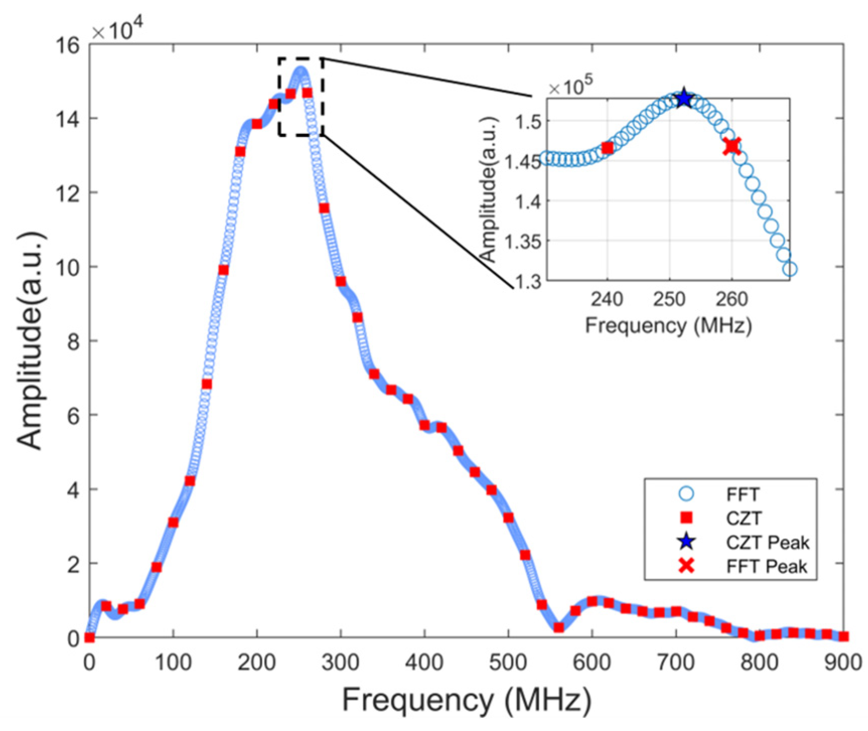
2.4.2. Chirp Z-Transform for Extracting Frequency-Domain Features

When using GPR for shallow subsurface detection, higher sampling points and shorter time windows are often employed in the acquisition settings to study the dynamic changes in electromagnetic waves over time more precisely, resulting in high temporal resolution. However, shorter sampling windows can lead to low frequency resolution in the spectrum when applying FFT, which can hinder the accurate extraction of frequency-domain features from GPR signals—“picket-fence effect”. The chirp Z-transform (CZT), on the other hand, allows for arbitrary precision sampling within a specified frequency band, enabling the extraction of more accurate features [36,43].

To demonstrate the effectiveness of using CZT to extract spectral features from GPR signals, a single-trace GPR signal was randomly selected and subjected to both FFT and CZT transformations. The sampling frequency was set to 2048 MHz, with the CZT frequency range spanning from 0 and 900 MHz, and 450 transformation points were employed. The results are presented in Figure 5. The spectral resolution of the FFT is limited by the sampling window length, resulting in a resolution of 20 MHz and a PF of 260 MHz. In contrast, CZT processing, while maintaining the spectrum calculated by FFT, successfully captured a higher-amplitude PF at 252 MHz between the 240 MHz and 260 MHz range, indicating that CZT can more accurately identify critical spectral features.

Based on previous research, this study selected the following seven frequency-domain features to comprehensively characterize the response of GPR signals to SVWC: PF, center frequency (CF); centroid frequency (CEF); frequency band energy (FBE); dominant frequency energy (DFE); and bandwidth energy percentage (BEP). The extraction methods for these features are summarized in

Table 1. Extraction of frequency-domain features.

Feature	Definition	Formula
PF	Frequency at which the power spectral amplitude is maximized	$PF=f_{p_{\max }}$
CF	Frequency at which the power spectral energy occupies half of the total energy	$CF=f_{{\displaystyle \frac{1}{2}}E}$
CEF	Weighted average frequency using the amplitude of the power spectral density as weights	$CEF={\displaystyle \frac{{\displaystyle {\int }_0^{+\infty }fP(f)df}}{{\displaystyle {\int }_0^{+\infty }P(f)df}}}$
FBE	Total energy within the frequency band	$FBE={\displaystyle {\int }_0^{+\infty }\left|P(f)\right|df}$
DFE	Maximum value of the power spectral density	$DFE=\left|\max (P(f))\right|$
BEP	Ratio of the power spectral density of a single frequency band to that of the total frequency band	$BEP={\displaystyle \frac{{\displaystyle {\sum }_{f_1}^{f_2}P(f)}}{FBE}}$

Note: $f$, denotes the frequency; $P(f)$, denotes the power spectral density corresponding to that frequency, which is the square of the amplitude.

[44].

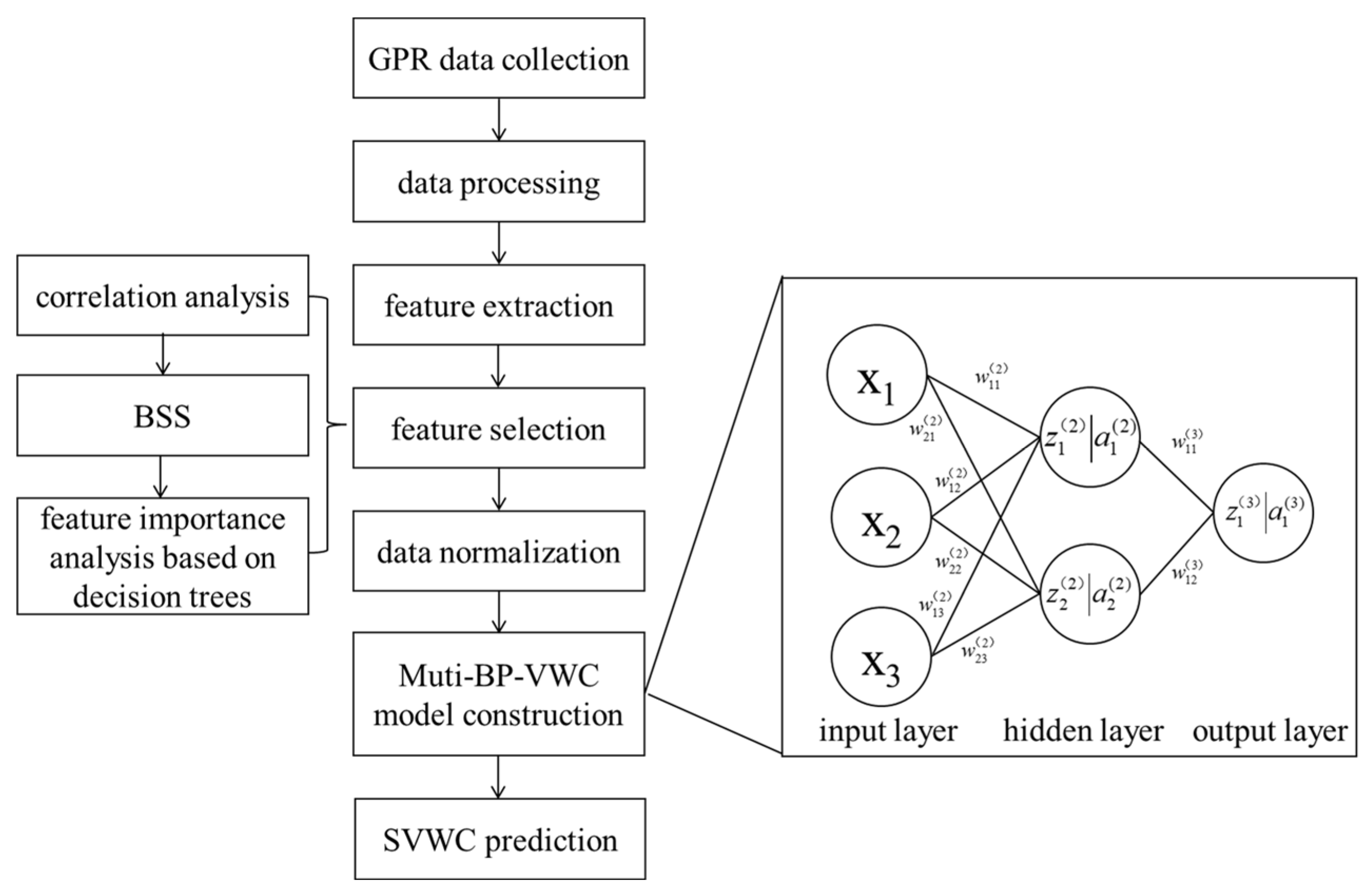
2.5. Construction of the SVWC Prediction Model Based on Multiple Signal Features

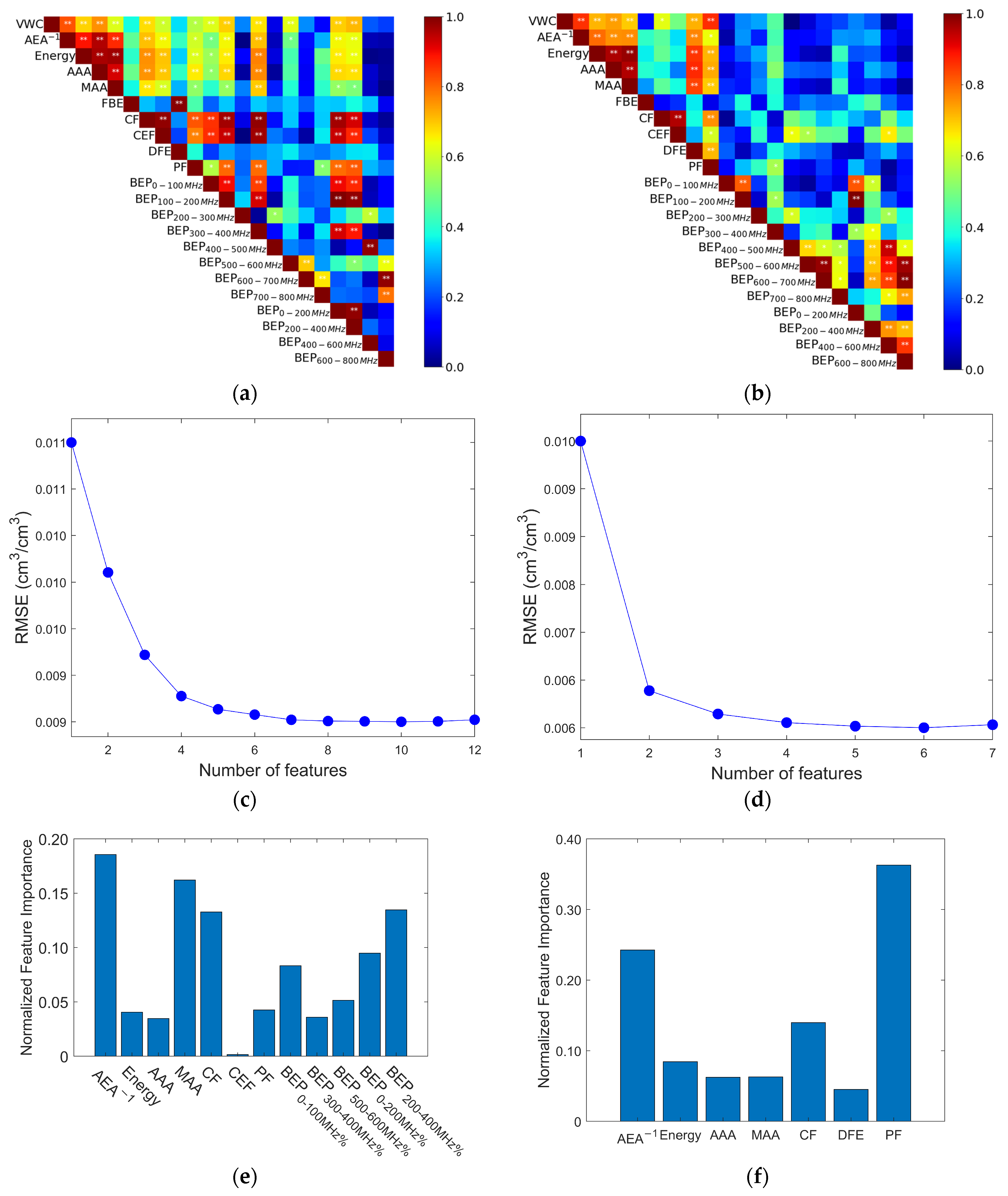
2.5.1. GPR Signal Features Selection

GPR signals exhibit a wide variety of features, but many of these features contain irrelevant variables with weak correlations to moisture content. Additionally, multicollinearity among these features may lead to data redundancy, negatively impacting model stability. Therefore, before constructing a multi-feature soil moisture prediction model, it is essential to select the most relevant features to obtain the optimal combination. The selection process involves the following three steps:

(1)

(Perform cross-correlation analysis and significance testing between SVWC and each feature, using the Pearson correlation coefficient to measure the linear relationship among variables [45].

(2)

Select the features that are significantly correlated with SVWC to form different feature sets and use the best subset selection (BSS) algorithm to plot the curve of the RMSE as a function of the number of features. The BSS algorithm evaluates all possible combinations of features [46,47]. Typically, the RMSE decreases rapidly with fewer features, and as the number of features increases, the rate of decrease in the RMSE slows down or levels off. Therefore, the optimal number of features is usually located at the inflection point where the RMSE begins to level off after a rapid decline.

(3)

Conduct a feature importance analysis based on random forests to evaluate the impact of each feature on the model’s prediction results and rank the features according to their importance [48].

2.5.2. BP Neural Network

The BP neural network is known for its strong capabilities in learning, memory, fault tolerance, nonlinearity, and adaptability. A three-layer neural network can effectively approximate any nonlinear continuous function and performs excellently when addressing problems with complex internal mechanisms [49,50], which is beneficial for capturing the nonlinear relationships between GPR signal features and SVWC. Moreover, the relatively simple structure of the BP neural network makes it computationally efficient, allowing for faster training and implementation even with limited resources.

The core structure of a BP neural network includes the input layer, hidden layers, and output layer. The input layer receives the raw feature data, the hidden layers perform nonlinear transformations on the data through neurons, and the output layer generates the prediction results. The number of neurons in the hidden layers determines the complexity of the model; more neurons help the network learn more complex patterns, but also increase the computational cost. The learning rate controls the size of the steps the model takes during the optimization process. A high learning rate can lead to poor convergence, while a low learning rate can cause the model to converge too slowly, potentially getting stuck in local minima. The activation function introduces nonlinearity into the model and the ReLU activation function is widely used in deep networks because it helps alleviate the vanishing gradient problem and improves training efficiency. By appropriately selecting these hyperparameters, the BP neural network can be better optimized and its prediction accuracy improved.

The BP neural network training process is divided into four main parts: data normalization, network design, forward propagation, and error backpropagation. A complete flowchart of the model’s construction is shown in Figure 6, which includes data collection, processing, and feature extraction, selection, and normalization. The GPR signal features are used as inputs, with the SVWC as the output and the BP neural network employed for training the Muti-BP-SVWC model.

The expression of the trained Muti-BP-SVWC model can be simplified as follows:

$$y=\sigma (W_3\cdot \sigma (W_2\cdot \sigma (W_1\cdot {\left[x_1,x_2\mathrm{\cdots }{x}_n\right]}^T+b_1)+b_2)+b_3)$$

(12)

where $W_1$, $W_2$, and $W_3$ represent the weight matrices from the input layer to the hidden layers and from the hidden layers to the output layer; the vectors $b_1$, $b_2$, and $b_3$ denote the bias vectors for each layer; $\sigma$ is the ReLU activation function; $\left[x_1,x_2\mathrm{\cdots }{x}_n\right]$ is the vector of GPR signal feature combinations; and $y$ is the predicted SVWC.

2.6. Performance Evaluation Criteria of the Models

The accuracy of the SVWC prediction model was evaluated using the determination coefficient (R²) and root mean square error (RMSE). R² reflects the proportion of total variability in the dependent variable that the model explains. Its value ranges from 0 to 1, with values closer to 1 indicating better predictive performance. The RMSE measures the difference between predicted values and actual values; a smaller RMSE value indicates a higher predictive accuracy of the model. R² and RMSE are defined as follows:

$$R^2={\displaystyle \frac{{\displaystyle \sum _{i=1}^n{(x_i-\overline{x})}^2{(y_i-\overline{y})}^2}}{{\displaystyle \sum _{i=1}^n{(x_i-\overline{x})}^2{\displaystyle \sum _{i=1}^m{(y_i-\overline{y})}^2}}}}$$

(13)

$$RMSE=\sqrt{{\displaystyle \frac{1}{n}}{\displaystyle \sum _{i=1}^n{(y_i-x_i)}^2}}$$

(14)

where $n$ represents the sample size; $x_i$ and $y_i$ denote the GPR signal features and SVWC sample values, respectively; and $\overline{x}$ and $\overline{y}$ are their corresponding sample means.

3. Results

3.1. Time-Domain Features

All the GPR signals near TDR measurement points in both the unmined and mined areas were extracted, and four time-domain features were obtained within the first positive half-cycle. Scatter plots of these features against TDR-measured SVWC were generated, and their correlation coefficients were calculated, as shown in Figure 7.

From Figure 7, it is evident that as SVWC increases, the energy and amplitude of the GPR signals exhibit an overall decreasing trend, while AEA⁻¹ is positively correlated with SVWC due to its reciprocal processing, indicating that the increase in SVWC leads to a rise in the soil’s dielectric permittivity, which enhances the attenuation of electromagnetic waves. Overall, in both areas, energy, AAA, MAA, and AEA⁻¹ all exhibit correlations with an SVWC above 0.60, demonstrating the potential of using time-domain features to estimate SVWC. Among these features, AEA⁻¹ has the strongest correlation with SVWC, reaching 0.82 in the mining area and 0.86 in the unmined area, suggesting that the envelope amplitude obtained after Hilbert transform is more sensitive to changes in SVWC and better captures these variations.

3.2. Frequency-Domain Features

The GPR signals near all TDR measurements in both the unmined and mined areas were subjected to CZT transformation, and various frequency-domain features were extracted. The correlation coefficients between these features and soil VWC were calculated, as shown in

Table 2. Correlation coefficient between GPR features of frequency-domain and SVWC.

Feature	Mined Area	Unmined Area	Feature	Mined Area	Unmined Area
FBE	−0.38	−0.13	BEP400–500MHz	0.09	−0.01
CF	−0.68	−0.63	BEP500–600MHz	0.63	0.08
CEF	−0.60	−0.49	BEP600–700MHz	0.26	0.16
DFE	−0.35	−0.72	BEP700–800MHz	−0.12	−0.20
PF	−0.57	−0.86	BEP0–200MHz	0.69	0.26
BEP0–100MHz	0.62	0.07	BEP200–400MHz	−0.71	−0.21
BEP100–200MHz	0.69	0.26	BEP400–600MHz	0.21	0.04
BEP200–300MHz	−0.26	0.29	BEP600–800MHz	0.19	0.11
BEP300–400MHz	−0.67	−0.46

. The features FBE, CF, CEF, DFE, and PF all exhibited negative correlations with VWC. The correlations between bandwidth energy percentages across different frequency ranges and VWC showed significant variation, primarily characterized by an increase in energy proportion in the low-frequency range and a decrease in the high-frequency range. This indicates that as soil moisture increases, the energy of electromagnetic waves gradually attenuates, and the spectral energy distribution shifts progressively toward lower frequencies.

Additionally, it was observed that in the unmined area, the energy proportion within the 200–300 MHz frequency range showed a positive correlation with SVWC, whereas in the mined area, it exhibited a negative correlation. This phenomenon suggests that the degree of spectral shift toward lower frequencies varies under different soil conditions.

To highlight the frequency shift phenomenon caused by the increase in SVWC, the amplitudes of the signals after CZT transformation were normalized, and the relationship between PF and SVWC was plotted. As shown in Figure 8, PF exhibits a general trend of shifting to lower frequencies as SVWC increases in both the unmined and mined areas. Within the same range of soil moisture content variation, peak frequencies in the mined area are more concentrated in the lower frequency range. This indicates that in the mined area, the scattering intensity of electromagnetic waves is greater, leading to more pronounced attenuation of high-frequency components.

3.3. Prediction of SVWC Using BP Neural Network

The SVWC, along with the corresponding GPR signal features from the two survey areas, was imported separately into SPSS (version 23.0) for cross-correlation analysis. The absolute value of the Pearson coefficient was used to assess the strength of the correlations among variables, and significance tests were conducted. As shown in Figure 9a,b, the variables that are highly significantly correlated with the SVWC in the mined area include AEA⁻¹, energy, AAA, MAA, CF, BEP_0–100MHz, BEP_100–200MHz, BEP_300–400MHz, BEP_500–600MHz, BEP_0–200MHz, and BEP_200–400MHz, while CEF and PF showed significant correlations. In the unmined area, the variables that are highly significantly correlated with SVWC include AEA⁻¹, Energy, AAA, MAA, DFE, and PF, with CF showing significant correlations.

Based on this, the BSS algorithm was employed to calculate the RMSE for different feature quantity combinations, evaluating their impact on model performance. As shown in Figure 9c,d, when the number of features was small, the RMSE decreased rapidly as additional features were introduced, indicating that adding features helps capture more information related to the target variable and enhances the model’s predictive capability. However, once the number of features reaches a certain threshold, the decrease in RMSE became less pronounced, suggesting that redundant information was being introduced into the model. Consequently, the optimal number of features for both the unmined and mined areas was determined to be four.

Finally, feature importance analysis based on random forest was used to quantify the importance of the selected features. The top four features were chosen as the final input variable combination. As shown in Figure 9e,f, the optimal feature combination for the mined area includes AEA⁻¹, MAA, BEP_200–400MHz, and CF, whereas for the unmined area, it consisted of PF, AEA⁻¹, CF, and energy.

After determining the optimal feature combinations, Muti-BP-SVWC models were constructed separately for the mined and unmined areas. To evaluate the accuracy, generalization ability, and practical application potential of the SVWC prediction models, the dataset was divided into a modeling set and a validation set. In the mined area, 12 data groups were randomly selected for modeling, while the remaining 5 groups were used for validation. In the unmined area, 9 data groups were randomly selected as the modeling set, with the remaining 5 groups serving as the validation set.

Because of the limited number of sample points in the study area, the statistical power of the dataset is constrained, making it difficult for the model to distinguish between data features and noise. Models trained on small datasets are prone to being overly sensitive to outliers and noise, leading the model to focus more on noise rather than general trends. After testing, it was found that directly using the raw data for training did not yield ideal prediction results. Therefore, we employed data augmentation by adding 0.01 times the level of noise to each feature parameter in the training set. This approach increased the training dataset size to three times the original, without significantly altering the physical meaning of the original features, in order to improve the model’s generalization ability. The validation set remained unchanged.

After data augmentation, considering the wide variety and significant dimensional differences among the radar feature parameters, all feature parameters in the dataset were normalized to ensure that each feature was within the same scale range. This step was taken to accelerate the model’s training process and improve its stability and convergence speed. After continuous adjustments, the final hyperparameters for the Muti-BP-VWC model in mined area were set as follows: a three-layer neural network with 2000 neurons in the input layer, 1000 neurons in the hidden layer, and 2000 neurons in the output layer, a learning rate of 0.01, and 1000 training iterations. For the Muti-BP-VWC model in unmined area, the hyperparameters were set as follows: a three-layer neural network with 800 neurons in the input layer, 200 neurons in the hidden layer, and 100 neurons in the output layer, a learning rate of 0.01, and 1000 training iterations.

To evaluate the performance of the Muti-BP-SVWC models, they were compared with SVWC prediction models built using the AEA method and frequency shift method on the same dataset, and their accuracy was assessed, as shown in

Table 3. SVWC prediction model accuracy evaluation.

Survey Area	Model	Modeling Set		Validation Set
		R2	RMSE (cm3/cm3)	R2	RMSE (cm3/cm3)
Mined area	AEA−1-SVWC	0.69	0.0112	0.60	0.0121
	PF-SVWC	0.30	0.0172	0.44	0.0143
	Muti-BP-SVWC	0.82	0.0086	0.77	0.0091
Unmined area	AEA−1-SVWC	0.76	0.0101	0.48	0.0106
	PF-SVWC	0.61	0.0119	0.81	0.0065
	Muti-BP-SVWC	0.90	0.0066	0.84	0.0059

. Figure 10 presents scatter plots of the validation set for each model. The closer the data points are to the 1:1 line, the higher the prediction accuracy of the model. In the mined area, the Muti-BP-SVWC model showed a significant improvement in accuracy over both the AEA method and frequency shift method in both the modeling and validation sets. In the modeling set, an R² was 0.82 and RMSE was 0.0086 cm³/cm³, while in the validation set, R² was 0.77 and RMSE was 0.0091 cm³/cm³. In the unmined area, the Muti-BP-VWC model demonstrated the best performance as well, with an R² of 0.90 and RMSE of 0.0066 cm³/cm³ in the modeling set, and an R² of 0.84 and RMSE of 0.0059 cm³/cm³ in the validation set. The PF-SVWC model also achieved good results, but it exhibited relatively lower accuracy in the modeling set and showed signs of overfitting.

3.4. SVWC Inversion of Study Area

This study aims to construct a soil volumetric water content (SVWC) prediction model using various early features of GPR signals, enabling rapid, accurate, and non-destructive detection of shallow surface soil moisture content across large areas, thus providing guidance for ecological restoration in mining areas. The Muti-BP-SVWC model developed in Section 3.3 was used to invert the soil moisture content in the mined and unmined areas. Kriging interpolation was applied to generate contour maps of the soil moisture content. For comparison, the TDR-measured soil moisture values were also plotted as contour maps. All images used the same color bar, as shown in Figure 11.

In both areas, the SVWC contour maps generated by TDR and GPR show similar trends. In the mined area, a noticeable region of soil moisture enrichment is observed in the southeast, with an overall trend of lower moisture in the west and higher moisture in the east. In the unmined area, the southern region exhibits soil moisture enrichment, with a general trend of higher SVWC in the south and lower moisture in the north. In localized regions, the GPR map shows more detailed distribution of local extreme values compared to the TDR map. This is because GPR is continuously collected with higher sampling point density and smaller intervals, reflecting variations in soil SVWC at a finer scale. For instance, a west-east high SVWC band is observed in the northern part of the central mined area, which is due to the area being an anticline, where moisture accumulates at the bottom due to gravitational forces. The TDR map fails to reflect this pattern because the distribution of TDR measurement points in this area is sparse, with large distances between points, leading to the replacement of regional moisture values by local moisture values.

The inversion results of GPR show that the soil moisture content in the mined area ranges from 0.040 cm³/cm³ to 0.131 cm³/cm³, with an average value of 0.071 cm³/cm³. In the unmined area, the soil moisture content ranges from 0.036 cm³/cm³ to 0.109 cm³/cm³, with an average value of 0.077 cm³/cm³. The shallow soil moisture content in the unmined area is slightly higher than in the mined area, possibly due to surface cracks from coal mining, which enhance water evaporation and lead to a decrease in soil moisture. However, because the study area is located in an arid region of western China, where the surface moisture is generally low, the average soil moisture content in the shallow surface layers of the unmined and mined areas differs by less than 0.01 cm³/cm³, indicating that the impact of coal mining on shallow soil moisture content is not significant.

4. Discussion

In analyzing the relationship between GPR signal features and SVWC, we found that an increase in soil moisture content intensifies the attenuation of electromagnetic waves, resulting in a decrease in the amplitude and energy of GPR signals, as well as an overall frequency shift toward the lower end of the spectrum. This aligns with previous research findings [22,26].

This indicates that linear models constructed using a single feature parameter are limited by their simplistic structure, making it difficult to fully capture the underlying information in the data. Conversely, under the same dataset, the Muti-BP-SVWC model demonstrates significantly improved accuracy and generalization capability in predicting soil moisture content. This suggests that the BP neural network, with its complex multi-layer structure, can integrate information from multiple features, effectively capturing the intricate nonlinear relationship between GPR signals and soil VWC, thereby enhancing overall predictive performance.

This study only establishes a relationship model between GPR signal features and soil VWC. However, the propagation characteristics of electromagnetic waves are also influenced by the soil’s physical properties, including bulk density, mineral composition, particle size, and porosity. The PF-VWC model performs significantly better in the unmined area compared to the mined area, likely due to the structural and compositional changes in the soil caused by mining activities and artificial maintenance. Mining processes lead to the development of shallow surface cracks and disturbances in soil layering, resulting in uneven moisture distribution. Additionally, the compaction effect of heavy machinery during the process of filling cracks alters soil surface particles and increases the bulk density, exacerbating soil heterogeneity. These changes make the dielectric properties of the soil more complex and uneven, thereby affecting the propagation characteristics of electromagnetic waves and weakening the linear relationship between PF and SVWC.

This research focuses on a very small area and compares it with a limited unmined region; future research can further explore this issue in the following ways: (1) conduct more field applications in different soil types to investigate the effects of soil properties such as bulk density, porosity, and other physical characteristics on GPR signals, thereby refining the soil moisture prediction model; (2) utilize GPR surveys both before and after coal mining in the same study area to analyze the extent of mining-induced impacts on soil moisture distribution.

5. Conclusions

This study proposed a method for constructing an SVWC prediction model by combining multiple GPR-derived feature parameters with a BP neural network, which improves the accuracy and stability compared to single-feature linear prediction models, enabling fast, accurate estimation of SVWC. The main conclusions are as follows:

(1)

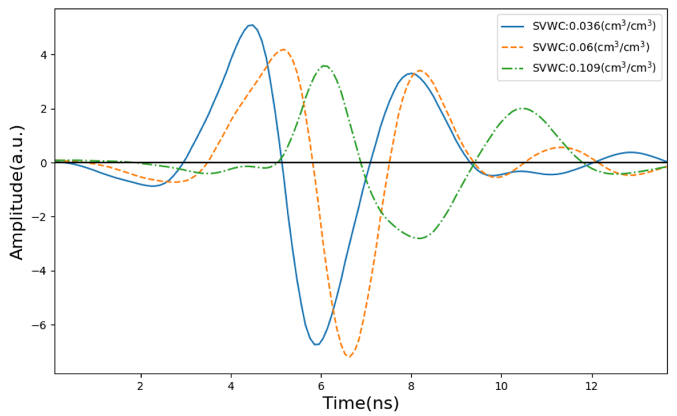
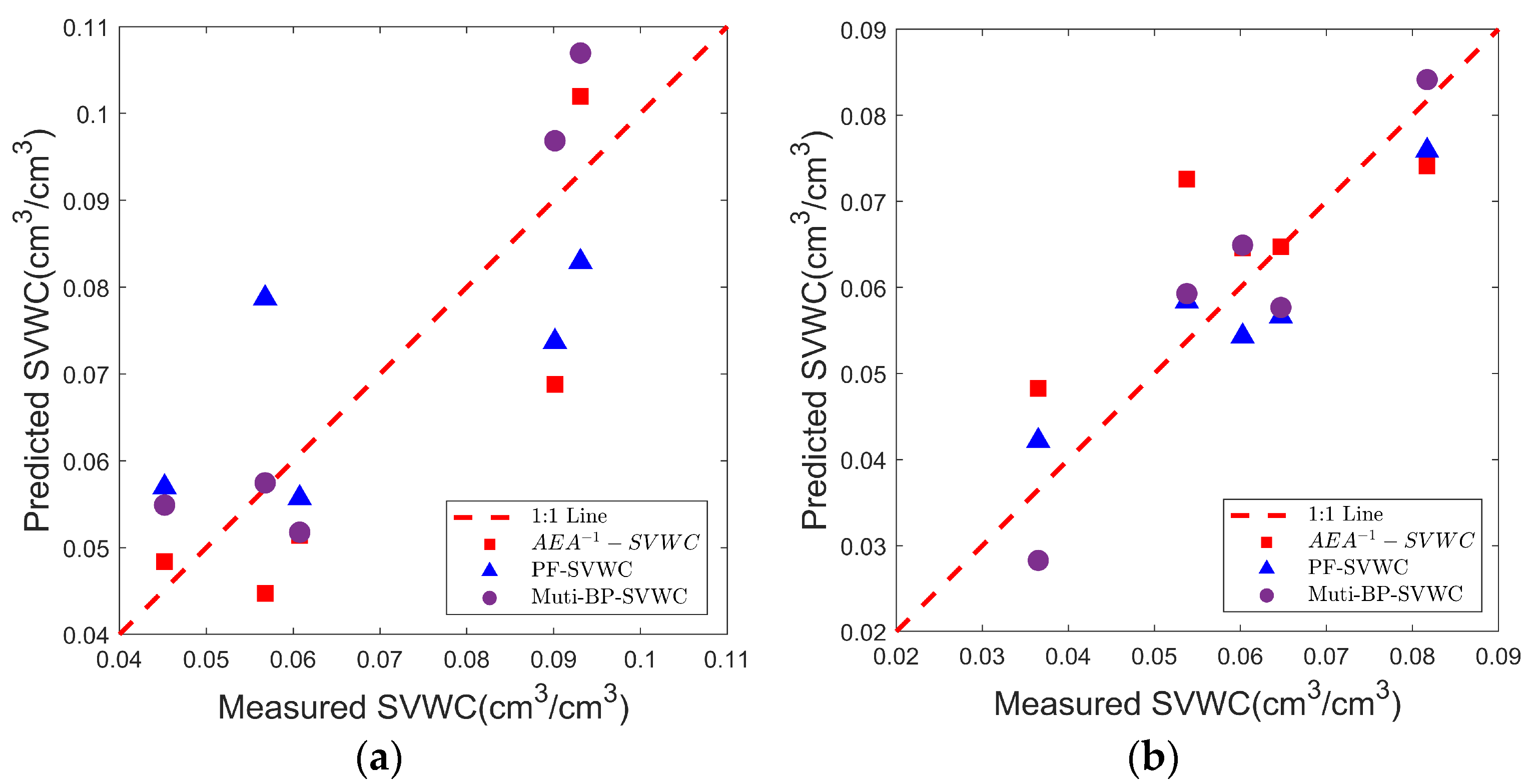
An increase in soil moisture leads to a decrease in the amplitude and energy of electromagnetic waves. Among the early GPR signal features, the AEA-1 parameter extracted from the first positive half-cycle of the signal better represents changes in SVWC compared to original time-domain features. The correlation coefficients between AEA-1 and SVWC in the unmined and mined areas reached 0.86 and 0.82, respectively, demonstrating improved predictive performance. The CZT transformation enables more precise extraction of frequency-domain features, revealing a shift of the spectrum toward lower frequencies as SVWC increases, with the shift being more pronounced in the mined area. However, the performance of the PF-based prediction model varies significantly under different soil conditions, with PF-SVWC correlations of 0.86 in the unmined area and 0.57 in the mined area.

(2)

The optimal feature parameter combination, identified through multiple feature selection methods, effectively reduces model complexity and minimizes redundant information. The Muti-BP-VWC model, compared to SVWC prediction models based on single-feature linear regression, significantly improves prediction accuracy. In the unmined area validation set, the model achieved an R² of 0.84 and an RMSE of 0.0059 cm³/cm³; in the mined area validation set, the R² was 0.77 and the RMSE was 0.0091 cm³/cm³. The model also demonstrated excellent generalization capability, making it suitable for SVWC inversion.

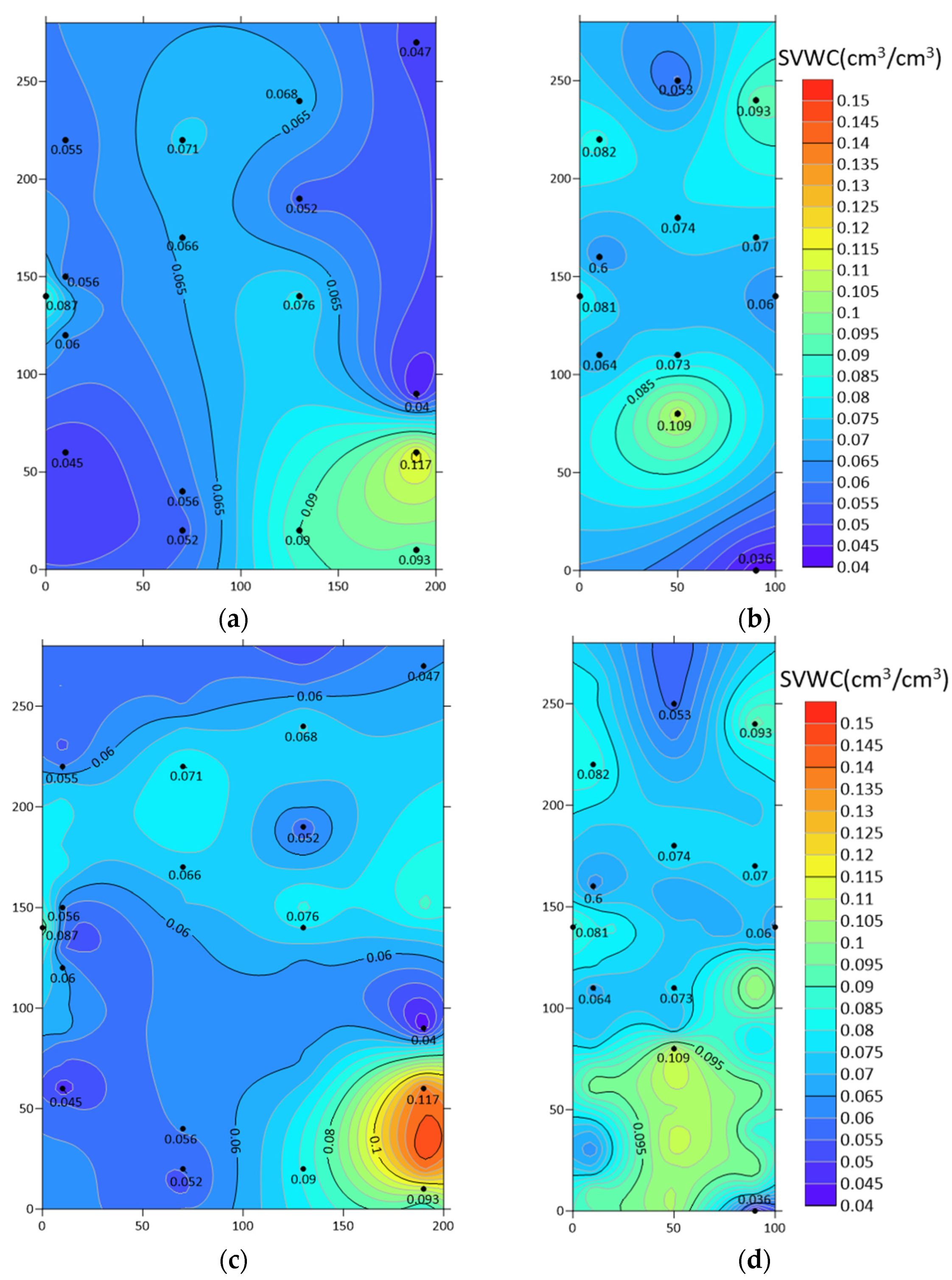
(3)

The SVWC contour maps derived from the Muti-BP-VWC model showed trends consistent with those measured by TDR. With its dense sampling points, GPR provided more detailed spatial distribution information on soil moisture in local regions, demonstrating its practical value in large-scale, rapid soil moisture detection. The inversion results indicated that the average SVWC difference between the mined and unmined areas was less than 0.01 cm³/cm³, suggesting that coal mining has minimal impact on shallow subsurface soil moisture.

References

1. Shen, X.; Foster, T.; Baldi, H.; Dobreva, I.; Burson, B.; Hays, D.; Tabien, R.; Jessup, R. Quantification of soil organic carbon in biochar-amended soil using ground penetrating radar (GPR). Remote Sens. 2019, 11, 2874. [Google Scholar] [CrossRef]
2. He, Y.; Fang, L.; Peng, S.; Liu, W.; Cui, C. A Ground-Penetrating Radar-Based Study of the Structure and Moisture Content of Complex Reconfigured Soils. Water 2024, 16, 2332. [Google Scholar] [CrossRef]
3. Wu, Z.; Xia, T.; Nie, J.; Cui, F. The shallow strata structure and soil water content in a coal mining subsidence area detected by GPR and borehole data. Environ. Earth Sci. 2020, 79, 500. [Google Scholar] [CrossRef]
4. Vereecken, H.; Huisman, J.; Bogena, H.; Vanderborght, J.; Vrugt, J.; Hopmans, J. On the value of soil moisture measurements in vadose zone hydrology: A review. Water Resour. Res. 2008, 44, 4. [Google Scholar] [CrossRef]
5. Robinson, D.A.; Campbell, C.S.; Hopmans, J.W.; Hornbuckle, B.K.; Jones, S.B.; Knight, R.; Ogden, F.; Selker, J.; Wendroth, O. Soil moisture measurement for ecological and hydrological watershed-scale observatories: A review. Vadose Zone J. 2008, 7, 358–389. [Google Scholar] [CrossRef]
6. SU, S.L.; Singh, D.N.; Baghini, M.S. A critical review of soil moisture measurement. Measurement 2014, 54, 92–105. [Google Scholar] [CrossRef]
7. Zhang, J.; Lin, H.; Doolittle, J. Soil layering and preferential flow impacts on seasonal changes of GPR signals in two contrasting soils. Geoderma 2014, 213, 560–569. [Google Scholar] [CrossRef]
8. Zreda, M.; Desilets, D.; Ferré, T.P.A.; Scott, R.L. Measuring soil moisture content non-invasively at intermediate spatial scale using cosmic-ray neutrons. Geophys. Res. Lett. 2008, 35, L21402. [Google Scholar] [CrossRef]
9. Peng, J.; Loew, A.; Merlin, O.; Verhoest, N.E. A review of spatial downscaling of satellite remotely sensed soil moisture. Rev.Geophys. 2017, 55, 341–366. [Google Scholar] [CrossRef]
10. Wang, L.; Qu, J.J. Satellite remote sensing applications for surface soil moisture monitoring: A review. Front. Earth Sci. China 2009, 3, 237–247. [Google Scholar] [CrossRef]
11. Cui, F.; Bao, J.; Cao, Z.; Li, L.; Zheng, Q. Soil hydraulic parameters estimation using ground penetrating radar data via en-semble smoother with multiple data assimilation. J. Hydrol. 2020, 583, 124552. [Google Scholar] [CrossRef]
12. Mahmoudzadeh, A.; Mohammad, R. Off- and on-ground GPR techniques for fieldscale soil moisture mapping. Geoderma 2013, 200, 55–66. [Google Scholar] [CrossRef]
13. Topp, G.C.; Davis, J.; Annan, A.P. Electromagnetic determination of soil water content: Measurements in coaxial transmission lines. Water Resour. Res. 1980, 16, 574–582. [Google Scholar] [CrossRef]
14. Zajícová, K.; Chuman, T. Application of ground penetrating radar methods in soil studies: A review. Geoderma 2019, 343, 116–129. [Google Scholar] [CrossRef]
15. Huisman, J.A.; Hubbard, S.S.; Redman, J.D.; Annan, A.P. Measuring soil water content with ground penetrating radar: A review. Vadose Zone J. 2003, 2, 476–491. [Google Scholar] [CrossRef]
16. Huisman, J.; Sperl, C.; Bouten, W.; Verstraten, J. Soil water content measurements at different scales: Accuracy of time domain reflectometry and ground-penetrating radar. J. Hydrol. 2001, 245, 48–58. [Google Scholar] [CrossRef]
17. Grote, K.; Hubbard, S.; Rubin, Y. Field-scale estimation of volumetric water content using ground-penetrating radar ground wave techniques. Water Resour. Res. 2003, 39, 1321. [Google Scholar] [CrossRef]
18. Klotzsche, A.; Lärm, L.; Vanderborght, J.; Cai, G.; Morandage, S.; Zörner, M.; Vereecken, H.; van der Kruk, J. Monitoring Soil Water Content Using Time-Lapse Horizontal Borehole GPR Data at the Field-Plot Scale. Vadose Zone J. 2019, 18, 190044. [Google Scholar] [CrossRef]
19. Huisman, J.A.; Snepvangers, J.J.J.C.; Bouten, W.; Heuvelink, G.B.M. Monitoring Temporal Development of Spatial Soil Water Content Variation: Comparison of Ground Penetrating Radar and Time Domain Reflectometry. Vadose Zone J. 2003, 2, 519–529. [Google Scholar] [CrossRef]
20. Pettinelli, E.; Vannaroni, G.; Di Pasquo, B.; Mattei, E.; Di Matteo, A.; De Santis, A.; Annan, P.A. Correlation between near-surface electromagnetic soil parameters and early-time GPR signals: An experimental study. Geophysics 2007, 72, A25–A28. [Google Scholar] [CrossRef]
21. Pettinelli, E.; Di Matteo, A.; Beaubien, S.E.; Mattei, E.; Lauro, S.E.; Galli, A.; Vannaroni, G. A controlled experiment to investigate the correlation between early-time signal attributes of ground-coupled radar and soil dielectric properties. J. Appl. Geophys. 2014, 101, 68–76. [Google Scholar] [CrossRef]
22. Di Matteo, A.; Pettinelli, E.; Slob, E. Early-time GPR signal attributes to estimate soil dielectric permittivity: A theoretical study. IEEE Trans. Geosci. Remote Sens. 2013, 51, 1643–1654. [Google Scholar] [CrossRef]
23. Ferrara, C.; Barone, P.; Steelman, C.; Pettinelli, E.; Endres, A. Monitoring shallow soil water content under natural field conditions using the early-time GPR signal technique. Vadose Zone J. 2013, 12, 1–9. [Google Scholar] [CrossRef]
24. Algeo, J.; Van Dam, R.L.; Slater, L. Early-Time GPR: A Method to Monitor Spatial Variations in Soil Water Content during Irrigation in Clay Soils. Vadose Zone J. 2016, 15, 1–9. [Google Scholar] [CrossRef]
25. LÜ, H.; NIE, J.; WANG, Z. Monitoring soil moisture content using early-signal of GPR amplitude. J. Soils 2022, 54, 169–176. [Google Scholar]
26. Benedetto, A. Water content evaluation in unsaturated soil using GPR signal analysis in the frequency domain. J. Appl. Geophys. 2010, 71, 26–35. [Google Scholar] [CrossRef]
27. Benedetto, A.; Benedetto, F. Remote Sensing of Soil Moisture Content by GPR Signal Processing in the Frequency Domain. IEEE Sens. J. 2011, 11, 2432–2441. [Google Scholar] [CrossRef]
28. Benedetto, A.; Tosti, F.; Ortuani, B.; Giudici, M.; Mele, M. Soil moisture mapping using GPR for pavement applications. In Proceedings of the 2013 7th International Workshop on Advanced Ground Penetrating Radar, Nantes, France, 2–5 July 2013; pp. 1–5. [Google Scholar]
29. Laurens, S.; Balayssac, J.P.; Rhazi, J.; Klysz, G.; Arliguie, G. Non-destructive evaluation of concrete moisture by GPR: Experimental study and direct modeling. Mater. Struct. 2005, 38, 827–832. [Google Scholar] [CrossRef]
30. Cui, F.; Wu, Z.; Wang, L.; Wu, Y. Application of the Ground Penetrating Radar ARMA power spectrum estimation method to detect moisture content and compactness values in sandy loam. J. Appl. Geophys. 2015, 120, 26–35. [Google Scholar] [CrossRef]
31. Lai, W.L.; Kind, T.; Wiggenhauser, H. A Study of Concrete Hydration and Dielectric Relaxation Mechanism Using Ground Penetrating Radar and Short-Time Fourier Transform. EURASIP J. Adv. Signal Process. 2010, 2010, 317216. [Google Scholar] [CrossRef]
32. Lai, W.L.; Kind, T.; Wiggenhauser, H. Using Ground Penetrating Radar and Time–Frequency Analysis to Characterize Construction Materials. NDT&E Int. 2011, 44, 111–120. [Google Scholar]
33. Lai, W.L.; Kind, T.; Kruschwitz, S.; Wöstmann, J.; Wiggenhauser, H. Spectral Absorption of Spatial and Temporal Ground Penetrating Radar Signals by Water in Construction Materials. NDT&E Int. 2014, 67, 55–63. [Google Scholar]
34. Zhang, S.; Zhang, L.; Ling, T.; Fu, G.; Guo, Y. Experimental research on evaluation of soil water content using ground penetrating radar and wavelet packet-based energy analysis. Remote Sens. 2021, 13, 5047. [Google Scholar] [CrossRef]
35. Bianchini Ciampoli, L.; Calvi, A.; D’Amico, F. Railway Ballast monitoring by GPR: A test-site investigation. Remote Sens. 2019, 11, 2381. [Google Scholar] [CrossRef]
36. Cheng, Q.; Zhang, S.; Chen, X.; Cui, H.; Xu, Y.; Xia, S.; Xia, K.; Zhou, T.; Zhou, X. Inversion of reclaimed soil water content based on a combination of multi-attributes of ground penetrating radar signals. J. Appl. Geophys. 2023, 213, 105019. [Google Scholar] [CrossRef]
37. Klewe, T.; Strangfeld, C.; Kruschwitz, S. Review of moisture measurements in civil engineering with ground penetrating radar–Applied methods and signal features. Constr. Build. Mater. 2021, 278, 122250. [Google Scholar] [CrossRef]
38. Li, Z.; Zeng, Z.; Xiong, H.; Lu, Q.; An, B.; Yan, J.; Li, R.; Xia, L.; Wang, H.; Liu, K. Study on Rapid Inversion of Soil Water Content from Ground-Penetrating Radar Data Based on Deep Learning. Remote Sens. 2023, 15, 1906. [Google Scholar] [CrossRef]
39. Li, X.; Cheng, X.; Zhao, Y.; Xiang, B.; Zhang, T. Deep Learning-Based Ground-Penetrating Radar Inversion for Tree Roots in Heterogeneous Soil. Sensors 2025, 25, 947. [Google Scholar] [CrossRef]
40. Zhang, X.; Zhao, X.; Li, S.; Lv, S.; Lin, C.; Wen, J. GPR-CUNet: Spatio-Temporal Feature Fusion Based GPR Forward and Inversion Cycle Network for Root Scene Survey. IEEE Sens. J. 2025, 25, 7569–7583. [Google Scholar] [CrossRef]
41. Lu, Q.; Liu, K.; Zeng, Z.; Liu, S.; Li, R.; Xia, L.; Guo, S.; Li, Z. Estimation of the Soil Water Content Using the Early Time Signal of Ground-Penetrating Radar in Heterogeneous Soil. Remote Sens. 2023, 15, 3026. [Google Scholar] [CrossRef]
42. Mie, G. Beiträge zur Optik trüber Medien, speziell kolloidaler Metallösungen. Ann. Phys. 1908, 330, 377. [Google Scholar] [CrossRef]
43. Ma, S.; Ma, Q.; Liu, X. Applications of chirp Z transform and multiple modulation zoom spectrum to pulse phase thermography inspection. NDT&E Int. 2013, 54, 1–8. [Google Scholar]
44. Xie, G.; Nie, J.; Chen, Z.; Xiong, Y.; Feng, Y.; Chen, D. Soil Moisture State Prediction Based on Ground Penetrating Radar Power Spectrum Properties Parameters. Water Saving Irrigation 2023, 10, 28–35. [Google Scholar]
45. Coscia, M. Pearson correlations on complex networks. J. Complex Netw. 2021, 9, cnab036. [Google Scholar] [CrossRef]
46. Wen, C.; Zhang, A.; Quan, S.; Wang, X. BeSS: An R Package for Best Subset Selection in Linear, Logistic and Cox Proportional Hazards Models. J. Stat. Softw. 2020, 94, 1–24. [Google Scholar] [CrossRef]
47. Hastie, T.; Tibshirani, R.; Tibshirani, R. Best subset, forward stepwise or lasso? Analysis and recommendations based on extensive comparisons. Stat. Sci. 2020, 35, 579–592. [Google Scholar] [CrossRef]
48. Menze, B.H.; Kelm, B.M.; Masuch, R.; Himmelreich, U.; Bachert, P.; Petrich, W.; Hamprecht, F.A. A comparison of random forest and its Gini importance with standard chemometric methods for the feature selection and classification of spectral data. BMC Bioinform. 2009, 10, 213. [Google Scholar] [CrossRef]
49. Zhang, Q.; Yu, H.; Barbiero, M.; Wang, B.; Gu, M. Artificial neural networks enabled by nanophotonics. Light Sci. Appl. 2019, 8, 42. [Google Scholar] [CrossRef]
50. Zador, A.M. A Critique of Pure Learning and What Artificial Neural Networks Can Learn from Animal Brains. Nat. Commun. 2019, 10, 3770–3777. [Google Scholar] [CrossRef]
Figure 1. Study area overview with GPR survey lines and TDR measurement points: (a) location map of study area; (b) Yushuquan coal mine; (c) mined area layout; (d) unmined area layout.
Water 17 00873 g001
Figure 2. A profile of ground-penetrating radar data.
Water 17 00873 g002
Figure 3. Amplitude of early time signals of GPR under different SVWC conditions.
Water 17 00873 g003
Figure 4. GPR signal, with the solid line indicating the first positive half-cycle: (a) amplitude of the GPR signal; (b) corresponding Hilbert transform of (a).
Water 17 00873 g004
Figure 5. A single-trace GPR signal was transformed using CZT and FFT. The spectrum obtained from the CZT transformation is represented by blue circles, with blue stars (★) indicating the peak frequencies extracted by CZT. The spectrum obtained from the FFT transformation is represented by red squares, with red crosses (✕) indicating the peak frequencies extracted by FFT.
Water 17 00873 g005
Figure 6. Flowchart of SVWC prediction using multiple GPR signal features combined with a BP neural network.
Water 17 00873 g006
Figure 7. Correlations between the time-domain features of the GPR signals and soil VWC. Blue circles represent samples from the mined area, and red circles indicate samples from the unmined area: (a) energy; (b) AAA; (c) MAA; (d) AEA−1.
Water 17 00873 g007aWater 17 00873 g007b
Figure 8. Frequency shift of GPR signal spectrum: (a) mined area; (b) unmined area.
Water 17 00873 g008
Figure 9. GPR signal features selection. The first column (a,c,e) shows the selection results for the mined area, while the second column (b,d,f) presents the results for the unmined area. The first row displays the cross-correlation analysis results between GPR features and moisture content, where * indicates a significant correlation and ** indicates a highly significant correlation. The second row contains the results of the BSS analysis, and the third row presents the feature importance score calculations.
Water 17 00873 g009
Figure 10. Scatter plots of SVWC prediction on validation set: (a) mined area; (b) unmined area.
Water 17 00873 g010
Figure 11. Contour maps of the SVWC. The first row (a,b) shows maps generated by TDR, and the second row (c,d) shows maps generated by GPR. The first column (a,c) represents the mined area, while the second column (b,d) represents the unmined area.
Water 17 00873 g011