Abstract
Taihu Lake is a large lake with high levels of eutrophication. Cyanobacterial outbreaks significantly affect the ecological environment and socioeconomic development. The chlorophyll-a (Chl-a) concentration, which is crucial for monitoring eutrophication, can be obtained through remote sensing inversion, and the random, sudden, and complex changes impose stringent requirements on the monitoring scale. However, single remote sensing images often fail to meet both the high temporal and spatial resolution requirements for Chl-a monitoring. This study took Taihu Lake as the research object, combined COMS-1 GOCI (1 h/500 m resolution) and Sentinel-2 MSI (5 d/10 m resolution) inverted Chl-a data, and developed a precorrection-based spatiotemporal downscaling method (PC-STDM). After eliminating systematic bias, the model used temporal weighting downscaling (TWD) and regression trend assessment downscaling (TRAD) methods to downscale the inverted Chl-a data, improving the temporal resolution of the Sentinel-2 MSI Chl-a inversion data from 5 d to 1 h. The verification resulted in an average R2 of 0.87 between the COMS-1 GOCI and Sentinel-2 MSI Chl-a data after adaptive correction. A comparison with the measured Chl-a data yielded a maximum fitting coefficient of 0.98, verifying the credibility of the model. The downscaled Chl-a concentration data detailed hourly changes and development trends, providing support for water quality monitoring in the Taihu Lake area.
1. Introduction
Eutrophication is the excessive input of nutrients into a body of water, leading to the excessive growth of aquatic plants and algae. It is currently a global environmental problem, posing serious threats to both aquatic ecosystems and human health [1]. The incidence of eutrophic lakes has been increasing worldwide since the 1960s [1], with this increasing trend being most pronounced in developing regions such as Asia and Africa [2]. By 2050, it is estimated that one-sixth and one-quarter of the world’s population will be at high risk of poor water quality due to excess nitrogen and phosphorus, respectively, making eutrophication one of the greatest threats to water quality [2]. Chlorophyll-a (Chl-a), a photosynthetic pigment present in all algae, is an important indicator of the degree of eutrophication of water bodies and can accurately reflect the abundance and biomass of aquatic plankton [3]. Therefore, timely and effective monitoring of Chl-a is of great significance for evaluating the water environment of Taihu Lake and for assisting in the management of water environments [4].
Traditional Chl-a monitoring methods include field sampling followed by laboratory analysis and in situ monitoring. The former requires both obtaining samples manually in water bodies and processing and analyzing the samples in laboratories, which is not only inefficient but also costly and time-intensive [5]. In situ monitoring automatically monitors Chl-a through preset underwater sensors, but it is easily affected by environmental factors such as the temperature and water composition. For example, waves caused by strong winds can cause the buoy of a monitoring station to shake, and water currents carrying suspended particles can dislodge sensors, leading to signal attenuation, and the performance of electronic components (such as photodiodes) fluctuates with temperature changes, among other factors, thereby reducing the monitoring accuracy [6]. The development of remote sensing technology has provided a new approach for the large-scale and dynamic monitoring of Chl-a concentrations in water environments [7]. It can frequently provide relatively accurate water quality information and is now widely used in the monitoring of Chl-a concentrations in lake water bodies. MODIS, MERIS, OLCI, and other main optical sensors perform well in monitoring Chl-a [8,9,10,11,12], despite some limitations in temporal and spatial resolutions [13].
In lake waters, the rapid proliferation of algae leads to a rapid increase in the Chl-a concentration. Under sustained specific environmental conditions (high temperatures, nutrient concentration, and stagnant water), the biomass of algae can increase by 2–3 times within 24 h [14], causing cyanobacteria blooms. To monitor and warn of this phenomenon in a timely manner, the monitoring frequency of Chl-a must be daily or even hourly. In addition, small lakes and areas infested with cyanobacterial blooms have high requirements for the spatial resolution of the monitoring data. Lekki et al. [15] pointed out that the minimum spatial resolution for accurately measuring changes in algae bloom concentrations in large lakes (area ≥ 500 km2) using remote sensing technology is 50 m, with a 25 m or higher resolution being the most suitable for identifying areas that have significant impacts on human health and ecological damage. It is currently believed that satellites such as Landsat (30 m resolution) and Sentinel-2 MSI (10 m resolution) can better meet spatial scale requirements [16]. However, most satellite data currently used for Chl-a monitoring do not meet the dual requirements for the monitoring time and spatial resolution. MODIS is widely regarded as a relatively accurate remote sensing data source [17]. However, its spatial resolution of 1 km hinders Chl-a monitoring in inland lakes and complex coastal areas. As a mainstream water color satellite, VIIRS has a revisit time as short as 14 h and has improved its spatial accuracy to a certain extent [18]. However, its minimum resolution of 750 m is still unsuitable for fine-grained monitoring. Landsat has great potential for estimating a variety of water quality parameters, with a spatial resolution of 30 m and good detection ability [19]. However, its 16-day revisit period makes Chl-a monitoring difficult. Sentinel-2 MSI has a higher spatial resolution than MODIS, Landsat, and VIIRS, among other factors, and can accurately monitor the process of Chl-a [20] development in algal blooms on a 5-day time scale. The geostationary ocean color imager (GOCI), launched in 2010 by the Korea Ocean Satellite Center (KOSC), has a temporal resolution of 1 h, which meets the need for monitoring dynamic changes in Chl-a [21]. However, its spatial resolution is coarse and is unable to satisfy the requirements for fine-grained monitoring.
To improve the data’s accuracy and meet the need for high-resolution monitoring, it is, therefore, necessary to use downscaling methods for data fusion. Downscaling is the process of converting low-resolution data into high-resolution data that can be applied to both spatial and temporal dimensions. Spatial downscaling methods are relatively common in remote sensing research. Wang et al. [22] proposed a spatial downscaling method for the GPM IMERG precipitation dataset, optimizing precipitation data with a spatial resolution of 11 × 11 km to 1 × 1 km; Chu et al. [23] used a random forest model to improve the spatial resolution of GRACE data from 300–400 km to 0.25 × 0.25 km based on three spatial downscaling ideas: grid point, watershed, and national scale. While retaining the characteristics of GRACE data, they obtained a refined water storage change situation. Nomura et al. [24] constructed a downscaling model based on a convolutional neural network (CNN) and used SAR data to increase the spatial resolution of MODIS NDVI products from 250 m to 10 m. Zhang et al. [25] proposed a Chl-a downscaling model based on multivariate analysis (MVA) and gradient boosting decision tree (GBDT), which increased the spatial resolution of Sentinel-3 Chl-a data from 300 m to 30 m, making it particularly suitable for inland lakes in different environments. Relevant studies have also been conducted on temporal downscaling. He et al. [26] proposed the SRF-MF method based on the random forest (RF) model, which uses satellite products to fuse station data and generate high-quality daily precipitation data. Adrien et al. [27] proposed an enhanced Delta method to improve the climate change index from a daily resolution to hourly resolution and verified the versatility of this method within a certain range.
In contrast, temporal downscaling is mainly applied in the fields of meteorology and climate. For water environment monitoring, especially for downscaling water quality parameters such as Chl-a, research is still limited. And the short-term analysis of remote sensing data still faces challenges in terms of accuracy and frequency. Although there are some daily or hourly satellite products, most studies have focused only on annual or monthly products, such as soil moisture and precipitation. These parameters change relatively slowly and have low temporal resolution requirements. This may be one of the reasons for the limited attention given to temporal downscaling in the current remote sensing field. Simultaneously, owing to the randomness, mutability, and complexity of Chl-a concentration changes, higher requirements are placed on its accuracy and frequency in water quality monitoring. Therefore, high-precision temporal downscaling research on water quality parameters such as Chl-a holds practical significance and application value.
To address these issues, this study proposed a precorrection-based spatiotemporal downscaling method (PC-STDM). This approach adaptively corrects the Chl-a concentration inversion data obtained from the Sentinel-2 MSI and the COMS-1 GOCI, and the Sentinel-2 MSI inversion data were temporally downscaled according to the calibrated COMS-1 GOCI hourly Chl-a concentration change trend to generate Chl-a concentration data with both a 10 m spatial resolution and a 1 h temporal resolution. This process achieves an effective fusion of Chl-a data at different scales, overcomes the resolution limitations of traditional remote sensing data, and can more accurately reflect the spatiotemporal variation characteristics of Chl-a in lake waters, providing reliable data support for water quality monitoring, ecological environmental assessment, and the construction of an early warning system in the Taihu Lake area.
2. Study Area and Data
2.1. Overview of the Study Area
Taihu Lake (30°55′40″–31°32′58″ N, 119°52′32”–120°36′10″ E) is the third largest freshwater lake in China and an important source of drinking water and fishery resources in the Yangtze River Delta region, covering an area of approximately 2427 km2. In recent years, with the increase in social and economic activities and irrational exploitation of lake resources, Taihu Lake is facing serious eutrophication problems, resulting in frequent outbreaks of cyanobacterial blooms, which have had a serious impact on the ecological environment and social economic development of Taihu Lake and its surrounding basins [28]. Since 1998, the total economic losses caused by cyanobacteria blooms in Taihu Lake reached RMB 46.5 billion, accounting for 5.9% of the region’s GDP [29], which has seriously restricted the sustainable development of the regional economy. Currently, Taihu Lake is one of the lakes with the most serious cyanobacteria bloom problem in China and is also one of the eutrophic water bodies that the country focuses on [30].
Taihu Lake (30°55’40″–31°32’58″ N, 119°52’32”–120°36’10″ E) is the third largest freshwater lake in China and an important source of drinking water and fishery resources in the Yangtze River Delta region, covering an area of approximately 2427 km2. In recent years, with the increase in social and economic activities and irrational exploitation of lake resources, Taihu Lake is facing serious eutrophication problems, resulting in frequent outbreaks of cyanobacterial blooms, which have had a serious impact on the ecological environment and social economic development of Taihu Lake and its surrounding basins [28]. Since 1998, the total economic losses caused by cyanobacteria blooms in Taihu Lake reached RMB 46.5 billion, accounting for 5.9% of the region’s GDP [29], which has seriously restricted the sustainable development of the regional economy. Currently, Taihu Lake is one of the lakes with the most serious cyanobacteria bloom problem in China and is also one of the eutrophic water bodies that the country focuses on [30].
2.2. Remote Sensing Data
This study used Sentinel-2 MSI and COMS-1 GOCI remote sensing data from the Taihu Lake area from 2019 to 1 May 2024. The two sensors complement each other in terms of temporal and spatial resolution, providing a data basis for downscaling.
Sentinel-2 MSI remote sensing data L2A products are atmospherically corrected surface reflectance products that can be downloaded from the Google Earth Engine (https://earthengine.google.com/, accessed on 13 March 2025) platform. The satellite consists of two constellations, Sentinel-2A and -2B, with a global revisit frequency of five days; a spatial resolution of 10 m; and 13 spectral bands, including several bands, B4, B5, B6, B7, and B8A, that are sensitive to Chl-a [31].
GOCI I and GOCI II remote sensing data were obtained from the Korea Ocean Satellite Center (https://www.nosc.go.kr, accessed on 13 March 2025), and two generations were launched. GOCI I, which provided the 2019–2020 data, was launched in 2010 and operated until March 2021. It contains eight bands, has a spatial resolution of 500 m, and provides observation data at eight moments per day with a time resolution of 1 h. GOCI II, which provided the 2021–2024 data, was launched in February 2020 and contained 13 bands, featuring a higher spatial resolution of 250 m. It captures data 10 times per day with a time resolution of 1 h and has excellent performance in water color inversion [32,33].
Because the atmospheric correction products provided by the Korea Ocean Satellite Center include land masking and cannot cover the Taihu Lake area, it is necessary to perform atmospheric correction on the L1B products. In this study, the atmospheric correction method was based on the Second Simulation of the Satellite Signal in the Solar Spectrum (6S) model, which is widely used in the atmospheric correction processing of COMS-1 GOCI data [34,35,36]. The specific correction method is as follows: first, the radiance of the image was calculated to obtain the Top of the Atmosphere (TOA) reflectivity and generate a preliminary reflectivity image; then, the Rayleigh scattering reflectivity was calculated using the 6S model and removed; finally, the TOA reflectivity after removing the Rayleigh scattering, path radiation reflectivity, downward transmission rate, and upward transmission rate of the atmosphere were integrated to derive the final surface reflectivity.
2.3. In Situ Measured Data
Validation data of the daily variation trend of Chl-a in Taihu Lake were obtained from the China National Surface Water Quality Automatic Monitoring Real-time Data Release System (https://szzdjc.cnemc.cn:8070/GJZ/Business/Publish/Main.html, accessed on 13 March 2025), with 1-hour or 4-hour sampling intervals. The measured data were collected using the fluorescence detection method: after the Chl-a molecule is excited by blue light, it emits longer-wavelength light (usually red light or near-infrared light), which is fluorescence. In the in situ measurement, the monitoring equipment emits blue light to excite the Chl-a in the water sample and detects the returned fluorescence signal. Based on the characteristic that the fluorescence intensity of Chl-a is proportional to its concentration, the concentration of Chl-a in the water can be calculated. However, the fluorescence signal is susceptible to interference from the water body (such as temperature, turbidity, and colored dissolved organic matter (CDOM)). A correction algorithm is usually used to adjust the measurement data to eliminate or compensate for the influence of these interfering factors. The hydrological monitoring data of the four monitoring sections from 2020 to 2023 (Table 1) were selected according to our data verification needs in this study. The section distribution and detailed information are shown in Figure 1.

Table 1.
Hydrological monitoring section information.
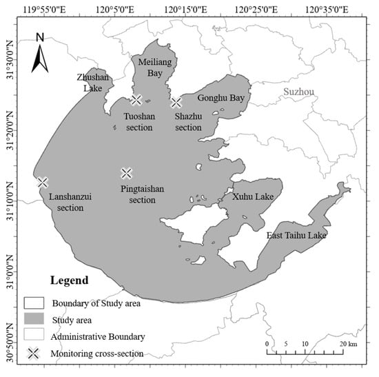
Figure 1.
Geographical location of the study area.
3. Methods
3.1. Project Research Framework
This study developed a spatiotemporal downscaling model based on a machine learning precorrection method. We used an empirical model to derive Chl-a concentrations from Sentinel-2 MSI and COMS-1 GOCI images with complementary spatial and temporal resolutions. The COMS-1 GOCI inversion data were adaptively corrected using a random forest model to reduce the deviation of the inversion results between different data sources. After correction, downscaling methods based on time weight and regression trend evaluation were used to extract the temporal characteristics of COMS-1 GOCI high-temporal-resolution inversion data and coupled with Sentinel-2’s high-spatial-resolution data to generate high-spatiotemporal-resolution Chl-a concentration data. Finally, the measured data were used to validate the accuracy of the daily variation trend of Chl-a concentration. The overall framework of this study is shown in Figure 2.
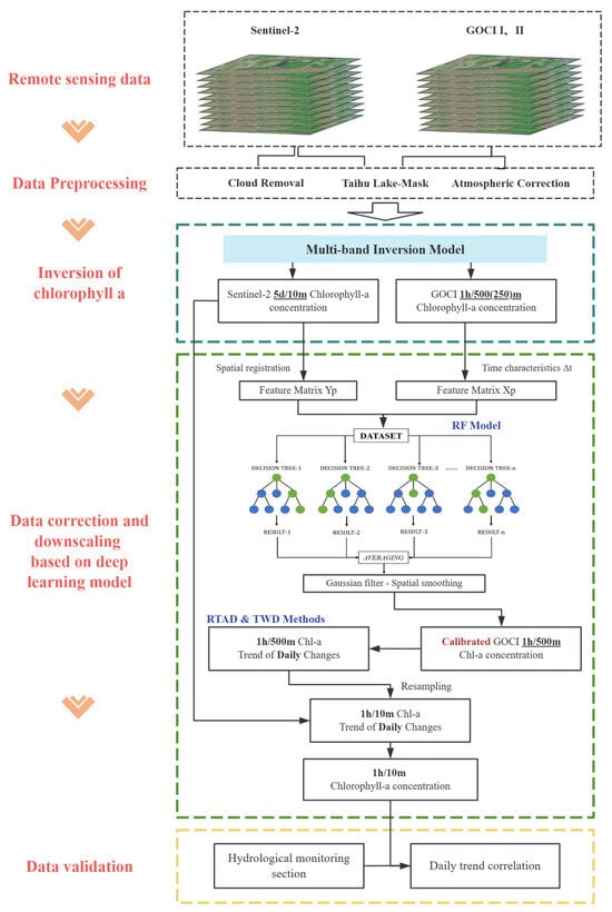
Figure 2.
Technology roadmap.
3.2. Chlorophyll-a Concentration Inversion
This study employs a multispectral remote sensing inversion model to achieve a quantitative estimation of the Chl-a concentration. In water environment remote sensing, satellite sensors can capture reflectance from the visible to near-infraredspectral range (400–900 nm). Based on the wavelength-specific absorption and scattering effects of Chl-a and coexisting substances on light of specific wavelengths, their specific spectral characteristics can be captured. Combined with the spectral characteristics of other optical components in the water body (such as suspended particulate matter and colored soluble organic matter, among other factors.), a multivariate reflectance combination relationship model for separating interference factors can be constructed. Based on the in situ calibration dataset, the model parameters are optimized, and a quantitative mapping relationship between reflectance and Chl-a concentration is established to achieve the estimation of Chl-a concentration. The specific inversion model is as follows.
3.2.1. COMS-1 GOCI Inversion Model
The Chl-a inversion of the COMS-1 GOCI remote sensing data adopted the three-band model expanded by Guo et al. [37], initially developed by Dall’ Olmo and Gitelson [38]. The formula is as follows:
where is the concentration of Chl-a after inversion correction; is the reflectance value at wavelength ; (680 nm) is in the Chl-a absorption peak band, (660 nm) is in the absorption valley band, and (745 nm) is located in the near-infrared band, which is used to eliminate the influence of backscattering.
The final fitting model is as follows:
The inversion model does not involve optical parameters and is easier to promote and apply [37]. This model introduced total suspended matter (TSM) and colored dissolved organic matter (CDOM) in the water body and included a lot of tests and calibrations, which can effectively eliminate the interference of turbid water in Taihu Lake on the inversion accuracy. It had good inversion performance, a low MAPE (0.463), and a high R2 (0.82) during model calibration and has been used to invert Chl-a in lake waters in Eastern China currently.
3.2.2. Sentinel-2 MSI Inversion Model
The Chl-a inversion of Sentinel-2 MSI remote sensing data adopted the four-band model proposed by Wang [39], which performed well, with an R2 value of 0.78. The model uses the fact that the absorption coefficients of total suspended matter (TSM) and colored dissolved organic matter (CDOM) in the two bands of 660–690 nm and 660–730 nm are very small to reduce the impact of TSM and CDOM and introduces the fourth band after 730 nm using as the new parameter to further reduce the interference of turbid water bodies. The final fitting model is as follows:
3.3. Temporal Downscaling of Chlorophyll-a Inversion Data
3.3.1. COMS-1 GOCI Chlorophyll-a Inversion Correction
Due to the differences between the Sentinel-2 MSI and COMS-1 GOCI remote sensing satellites in terms of orbital configurations, observation time, instrument parameters, and band settings, the source data obtained in this study exhibit systematic discrepancies (Table 2). The Sentinel-2 satellite is designed for inland environmental monitoring, and its multispectral instrument (MSI) can provide a unique spectral band suitable for the quantification of Chl-a [40]. The COMS-1 GOCI satellite is designed for ocean monitoring and performs well in ocean observations, but its application in complex water bodies, such as inland lakes, is not as good as that of Sentinel-2 MSI. The differences in subsequent atmospheric correction processing methods and inversion models further magnified the deviation between Sentinel-2 MSI and COMS-1 GOCI inversion data. In addition, in the comparison of Chl-a inversion data with the measured data of the water quality monitoring sections, the COMS-1 GOCI Chl-a inversion concentration was generally higher, while Sentinel-2 retrievals showed good agreement.
Table 2.
Data deviations between Sentinel-2 and COMS-1 satellites.
The proposed downscaling method was based on the idea of trend acquisition and data fusion. The large difference between the two data sources causes the daily variation trend obtained in the COMS-1 GOCI inversion results to not match the fusion process with Sentinel-2 MSI, affecting the reliability of the final product. Therefore, it is necessary to pre-correct the COMS-1 GOCI inversion results to bring the COMS-1 GOCI closer to Sentinel-2 MSI, which had a better inversion effect.
To this end, this study proposed an adaptive bias correction method based on a random forest model. This method established a nonlinear mapping relationship with time adaptability through multilayer feature analysis and an ensemble learning strategy. Experimental results showed that this method can not only effectively reduce the system error but also maintain the temporal dynamic characteristics of the COMS-1 GOCI inversion data. The process of adaptive correction included three parts: spatial registration, feature construction, and model structure construction.
Considering the difference in spatial resolution between COMS-1 GOCI and Sentinel-2 MSI data, spatial registration was required first. Let the COMS-1 GOCI data matrix be , and the Sentinel-2 MSI data matrix be , where b is the number of bands (1 in this study, indicating Chl-a concentration); and are the height and width dimensions of the two types of data, respectively. Sentinel-2 MSI data were resampled using the bicubic interpolation method.
where is the Sentinel-2 MSI data matrix, is the Sentinel-2 MSI resampled data matrix, and represents the bicubic interpolation resampling function, which ensures that the two types of data have the same spatial resolution and georeference.
After obtaining the registered dataset, a feature vector was constructed for each grid point of the COMS-1 GOCI inverted Chl-a data, and the inverted data of Sentinel-2 MSI was used as the corresponding target vector. The image data were reorganized into a feature matrix to establish an effective mapping relationship. Simultaneously, to retain the daily variation trend of the COMS-1 GOCI inversion results, the difference in transit time () between the Sentinel-2 MSI (UTC 3:00) and COMS-1 GOCI was considered in the inversion model training process. The time difference feature () as the model input enable the model to take into account the influence of the observation time on the inversion results, maintain the time continuity of the data to a certain extent, and make the model’s correction of data at different time points continuous and smooth, without sudden changes or distortions in the median of the time series.
The random forest model was an integrated learning system comprising T-decision trees. Each decision tree used a recursive binary method to divide the feature space through node impurity measurement (using the mean square error method), partition parameters, and a number of samples of the left and right child nodes. The output was the average of the prediction results for all decision trees. To process large-scale remote sensing data, model training was performed to adopt a batch processing strategy. When the data volume exceeded the threshold, the dataset was divided into batches and processed separately. Finally, Gaussian filtering was applied to the output results for spatial smoothing, which indirectly enhances the stability of the time series. This processing method assumes that the spatial variation trends of adjacent regions have certain similarities, which helps to suppress abnormal fluctuations and make the time trend more reliable.
In this study, the model training adopted multithreaded parallel training with 100 decision trees, a random selection of features ( total number of features), and a minimum leaf node sample number of 5. The mean absolute percentage error () and determination coefficient () were used to evaluate the model performance.
3.3.2. Sentinel-2 MSI Chlorophyll-a Temporal Downscaling
The variation characteristics of Chl-a concentration vary under different aquatic environments, which necessitates different requirements for downscaling methods. On the one hand, in open waters, where the water body is deeper, the mixing of waves and currents in open waters is more sufficient, making the spatial distribution of Chl-a concentration more uniform and the daily variation trend of Chl-a concentration relatively stable, requiring the downscaling method to have the ability to capture the pattern of this trend change; in contrast, the water body in bays and other areas has restricted hydrodynamic activity and prolonged residence times, which makes it easy to induce localized stagnation and nutrient accumulation. It is also greatly affected by human activities and river input, making the Chl-a changes exhibit high complexity. So, it is necessary to improve the ability of downscaling methods to capture mutation while minimizing the impact of certain abnormal concentration values on the overall results during the study period.
Based on the above requirements, this study used two methods, regression trend assessment (RTAD) and time weight (TWD), to perform temporal downscaling on the Chl-a inversion data. While retaining the accurate spatial characteristics of Sentinel-2 MSI, the temporal variation characteristics of COMS-1 GOCI were integrated to extrapolate the Chl-a concentration data with a temporal resolution of 1 h and a spatial resolution of 10 m. The study verified the reliability of the two methods and included a multi-dimensional analysis of the reasons for the differences in the methods, improving the overall applicability of the model, providing more accurate Chl-a concentration downscaling methods for different types of waters, and addressing operational requirements for water quality surveillance in the Taihu Lake area.
- Regression-based Trend Assessment Downscaling Method (RTAD)
In the downscaling method based on regression trend assessment, the study used COMS-1 GOCI data at different hours of the day to perform pixel-by-pixel regression analysis, with time as the independent variable and Chl-a concentration as the dependent variable, fitting three models: linear regression, quadratic trend regression, and Theil-Sen fitting (robust regression). The regression equation is as follows. The goodness of fit was evaluated for each pixel by calculating the regression model R2, and the best regression equation under the daily trend of the pixel was selected.
where represents the COMS-1 GOCI data at time ; are the regression model coefficients obtained by fitting.
The equation coefficients were stored in the form of raster data, and the trend raster data were resampled to the Sentinel-2 MSI data scale using the nearest neighbor method:
where is the target grid position; the coordinates of the neighboring grid with the closest Euclidean distance; is the value of the grid before resampling; is the value of the grid after resampling.
To adjust for systematic differences between COMS-1 GOCI and Sentinel-2 MSI, first for each grid , the value of COMS-1 GOCI at the reference time (i.e., the time of Sentinel-2 MSI transit, UTC 3:00) is calculated:
where is the reference value of the grid ; is the predicted value of the fitting function of the grid at the corresponding time ; is the reference time, that is, UTC 3:00.
Then, the ratio between the predicted value of the COMS-1 GOCI benchmark time and the inversion result of Sentinel-2 MSI was calculated as
where is the proportional relationship between the COMS-1 GOCI benchmark value and the Sentinel inversion result in the grid; is the value of the Sentinel-2 MSI inverted Chl-a result in the grid ; is the benchmark value of the grid .
The overall prediction value was adjusted based on the proportional relationship to retain the spatial characteristics of the Sentinel-2 MSI inversion results in the resulting data. Finally, time series interpolation was performed for each time and each grid to complete the data extrapolation of the Sentinel data within the COMS-1 GOCI time range.
where is the extrapolated data of the grid at time ; is the predicted value of the fitting function of the grid at the corresponding time ; is the proportional relationship between the COMS-1 GOCI benchmark value and the Sentinel inversion result in the grid , which is used to adjust the system difference.
- 2.
- Time-weighted downscaling method (TWD)
In the downscaling method based on time weight, the study used COMS-1 GOCI data at different hours of the day to calculate the grid-by-grid time weight, that is, , the ratio between the COMS-1 GOCI inverted Chl-a concentration data at each time point and the base time (UTC 3:00) data, was applied the weight to the Chl-a concentration data inverted by the sentinel, along with smoothing at the same time. The weight equation is as follows:
where represents the COMS-1 GOCI data at time ; is the base time (UTC 3:00); is the time weight, which reflects the ratio between the time point and the base time.
The temporal weights were stored in the form of raster data, and the weighted raster data were resampled to the spatial scale of the Sentinel-2 MSI data (10 m resolution) using the nearest neighbor method. The resampling formula is as follows:
where is the target grid; are the coordinates of the nearest neighbor grid with the Euclidean distance; is the value of the grid before resampling; is the value of the grid after resampling. The nearest neighbor method assigns the value to the target grid by selecting the closest grid; therefore, no weighted average is performed.
To reduce the noise that may be introduced during the resampling process, Gaussian filtering was used to smooth the resampled weight image. The formula is
where is the resampled weight image; is the smoothed weight image; is the standard deviation of the Gaussian filter, which controls the degree of smoothing. Larger values produce stronger smoothing effects and help remove noise.
Finally, the smoothed weighted image was multiplied by the Sentinel-2 MSI image to calculate the temporal downscaling result of the Sentinel data at the corresponding time :
where represents the inverted image data of the Sentinel image at time ; is the weighted image after smoothing; are the Chl-a data corresponding to the time after time downscaling. Through the time weight , the time variation characteristics of the COMS-1 GOCI Chl-a inversion results are combined with the sentinel inversion data to complete the data extrapolation of the sentinel data within the COMS-1 GOCI time range. Data downscaling corresponding to the COMS-1 GOCI transit time point is achieved.
3.4. Accuracy Assessment of Downscaling Data Based on In Situ Measured Data
This study used observed data from the Taihu Lake hydrological monitoring sections (Table 1) to evaluate the accuracy of the downscaled Chl-a data. The dynamic process of lake water is complex. Due to the combined effects of wind, water flow, algae aggregation, and other factors, the spatial distribution of Chl-a often shows significant differences. As the water body of Taihu Lake is relatively shallow, wind and waves can induce sediment resuspension in the water body while promoting horizontal algal drift, causing algae aggregation and significantly increasing the local Chl-a concentration [41]. The flow of water bodies causes a horizontal diffusion effect on the lake, causing the Chl-a concentration to show a frontal gradient change in estuaries or areas with significant lake flow (such as Meiliang Bay, Taihu Lake) [42]. These dynamic changes in water bodies cause uneven distribution of Chl-a, resulting in numerical discrepancies between single-point hydrological stations and remote sensing inversion data that measure the average value of the surface water area. At the same time, considering the differences in time and space between field hydrological stations and remote sensing data, this study includes the notion that there are certain limitations in comparing the downscaling results with the absolute values of the station measured data. Therefore, this study proposed a validation method based on variation trends. The key concept is to disregard the systematic deviation between the absolute values of the downscaled Chl-a inversion values and the site-measured values and focus on the temporal variation trend of Chl-a concentration after downscaling. If the downscaled results can accurately reflect the daily variation characteristics of Chl-a concentration similar to the site-measured data, the downscaling method can be considered credible.
First, the Chl-a data were spatially aligned with the measured data. A grid window of the size around each station was obtained. If more than 50% of the pixels in the window contained valid values, the window was considered valid, and the average value of the data in the window was calculated as the Chl-a concentration value ; if the window was invalid, it slid the window in other directions according to the algorithm until a valid window was obtained or the area was exceeded.
Next, the measured values and downscaled data of the stations were normalized.
where is the normalized result; is the original data; and are the minimum and maximum values of the data, respectively.
The two normalized sets of data were fitted using cubic polynomials:
where is the inverted value or measured value of Chl-a; is the sampling time (hours); are the fitting coefficient.
Finally, the trend correlation between the two was evaluated. A total of 100 points were sampled at equal intervals within the time range of [6:00, 18:00] Beijing time, and the Pearson correlation coefficient of these points was calculated as the fitting coefficient to evaluate the accuracy of the daily trend of the Chl-a inversion value after downscaling while calculating significance statistics to determine the credibility of the fitting coefficient r:
4. Result
4.1. Correction of Chlorophyll-a Inversion Data
Sentinel-2 MSI and COMS-1 GOCI images of the Taihu Lake area (2019–2024) were screened for visual quality; images with no obvious cloud cover and high-value areas of the inversion results coinciding with the algal bloom areas of the true-color images at the same time were selected to construct a dataset. A total of 92 Sentinel-2 MSI images and 627 COMS-1 GOCI images were selected.
Due to differences in data sources, preprocessing methods, and inversion models, the spatial distribution of the Chl-a concentration data inverted using COMS-1 GOCI and Sentinel-2 MSI exhibited seasonal discrepancies (Figure 3). In spring (Figure 3a) and winter (Figure 3d), the high-value areas of Chl-a were mainly concentrated on the west and south sides of the lake. According to the inversion values of Sentinel-2 MSI and the measured values, the highest concentrations of Chl-a in the high-value areas can reach approximately 30 μg/L and 45 μg/L during spring and winter, respectively, and those in the low-value areas are relatively low, in the range of 0–10 μg/L in both two seasons. The spatial patterns of the COMS-1 GOCI data before correction were roughly correlated with those of Sentinel-2 MSI, which reflected the spatial heterogeneity of Chl-a, but the inversion values were generally high, reaching 550 μg/L at the highest concentration and 17 μg/L at the lowest concentration. The maximum deviation reached 18 times the inversion value of Sentinel-2 under the same conditions. In summer (Figure 3b), Chl-a exhibited proliferation along western zones and spread to the center of the lake, with a maximum concentration of 50–70 μg/L. However, the COMS-1 GOCI Chl-a data before correction did not adequately capture the scope of the large-scale explosion. Instead, it showed extremely high values (approximately 550 μg/L) sporadically on the northwest coast. The overall spatial distribution was poor. The corrected COMS-1 GOCI inversion data (Figure 3(b3)) effectively restored the spatial characteristics of this large-scale explosion. In autumn (Figure 3c), there were occasional high-value areas of Chl-a on the northwest and north coasts, with the highest value in the range of 40–50 μg/L and the average value in the range of 5–10 μg/L. The COMS-1 GOCI data before correction covered almost the entire lake in the high-value area, with the highest reaching 760 μg/L, and even negative values in the low-value area. The corrected inversion data (Figure 3(c3)) solved the problems of disordered spatial distributions and negative values.
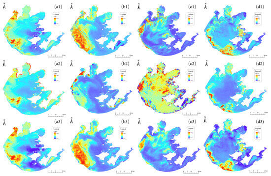
Figure 3.
Comparison of Chl-a inversion data for Sentinel-2 MSI. (1) COMS-1 GOCI before correction (2) and after correction (3) in spring (a1–a3), summer (b1–b3), autumn (c1–c3), and winter (d1–d3).
The above information demonstrates that there are serious inconsistencies between the inversion data from COMS-1 GOCI and Sentinel-2 MSI. This inconsistency was reflected in the large deviation of values in winter and spring, and in the summer and autumn, when algal blooms were more serious; it was reflected in the double deviation of spatial distribution and values, which was more serious. Therefore, before the actual downscaling process, this study first corrected the inversion data. While correcting the Chl-a values of COMS-1 GOCI to the inversion data of Sentinel-2 MSI, the daily variation characteristics of Chl-a were retained, providing better data preparation for subsequent downscaling work.
After correction, the COMS-1 GOCI inversion data were validated against Sentinel-2 MSI data at the same time, and the scatter plot is shown in Figure 4. It can be seen that the pre-corrected COMS-1 GOCI and Sentinel-2 MSI inversion results in different seasons showing large deviations, with the most severe deviations in summer. After model correction, the consistency of the data was significantly improved, the coefficient of determination (R2) increased to above 0.9, and the correction effect was obvious. The verification results showed that the highest value of R2 reached 0.93, with an average value of 0.87, indicating that the machine learning model correction used in this study effectively reduced system bias and improved the reliability of the data.
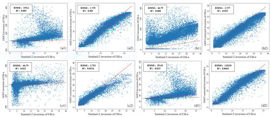
Figure 4.
Scatter plot of the fit degree between the corrected and uncorrected COMS-1 GOCI inversion data and Sentinel-2 MSI data. (1, 2) Uncorrected and corrected (unit: μg/L); (a1–d2): spring, summer, autumn, and winter.
4.2. Method Performance Comparison
When temporally downscaling the Chl-a inversion results of Sentinel-2, in order to adapt to the differences in chlorophyll changes under different environmental characteristics, this study used two methods: regression trend assessment downscaling (RTAD) and Time Weight Downscaling (TWD), to temporally downscale the Chl-a inversion data. In order to specifically compare the model performance and adaptability to the environment, this study conducted the following analysis based on the model principle.
The RTAD method used the GOCI daily variation data to fit the trend equation, which was later used to extrapolate the Chl-a concentration data from Sentinel-2 at different times of the day. However, this downscaling result based on the temporal trend assessment method exhibits strong functional dependence on the constructed trend equation. In order to judge the overall performance of the RTAD method, the accuracy of the trend equation in different seasons is quantitatively statistically analyzed, and the results are shown in Figure 5.
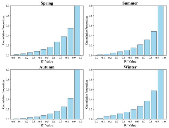
Figure 5.
R2 distribution of the fitting trend equation of the daily variation of Chl-a in each season using the RTAD method.
As can be seen in the figure, the overall R2 of the daily trend fitting equation of the RTAD method is relatively high, which exceeded 0.9 in over 50% of cases. Among the four seasons, autumn demonstrates the best fit to the overall trend, likely attributed to its relatively stable meteorological conditions and gentle hydrological variations. These favorable environmental factors promote Chl-a accumulation, resulting in a more concentrated and stable distribution of Chl-a concentrations that facilitates model fitting. In contrast, the method exhibits its lowest R² values in winter, possibly because the lower Chl-a values and less pronounced seasonal variations during this period reduce the model’s sensitivity to parameter changes.
In addition, in order to evaluate the significance of the regression model fitting of the RTAD method, the significance analysis was conducted. The t-test assessed linear/quadratic fits, while the Mann–Kendall test evaluated Theil–Sen regression. The statistically significant fitting part (p < 0.05) accounted for 57.24%, of which the p < 0.01 part accounted for 36.61%, which was within the acceptable range.
The TWD method uses the ratio of the benchmark time data to the target time data as the time weight to extrapolate the downscaled data. While independent of current remaining time data, this approach suffers from strong dependence on the quality of the benchmark time data. It can be observed in Figure 6 that the downscaled data restore the spatial characteristics of the Sentinel-2 inversion results and the time trend of the GOCI inversion results well, but some irregular noise artifacts are generated in the image. This is because the TWD method relies on the weight value of the Chl-a data of the benchmark time and the target time, which makes the data quality of the downscaled results have a greater correlation with the quality of the benchmark data. If there is noise in the GOCI data at the benchmark time point, the downscaling results of the TWD method inherit or even amplify the characteristics of this noise, leading to instability in output quality.
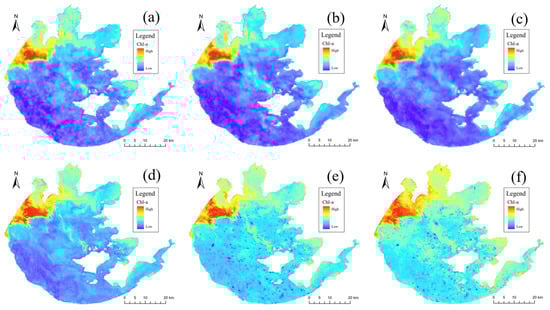
Figure 6.
Comparison of the downscaling results of the benchmark data and the TWD method. (a–c) The COMS-1 GOCI corrected data at 11:00, 14:00, and 16:00 local time, respectively. (d) The Sentinel Chl-a inversion data at 11:00 local time. (e,f) The downscaling results at 14:00 and 16:00 local time, respectively.
4.3. Accuracy Verification
This study selected the measured data of hydrological monitoring sections at four different locations in Taihu Lake from 2020 to 2023 to validate the downscaling results. The reliability of the downscaling method was confirmed by comparing the daily variation trend of the downscaling results with the measured data. Figure 7 shows the verification results for sections in different seasons and locations.
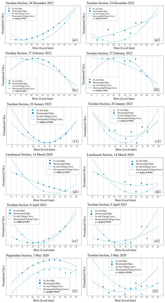
Figure 7.
Comparison of daily trends of measured and downscaled Chl-a concentrations (normalized to the range of 0–1) using (1) RTAD and (2) TWD methods in (a1–f2) typical dates from different seasons and sections.
As shown in Figure 7, the daily variation trend of the Chl-a concentration obtained using the two downscaling methods was consistent with the measured trend. Among all samples, the fitting coefficient r reached 0.98 and 0.96 at the highest, and it performed well at monitoring sections at different locations, indicating that the downscaling method proposed in the study can provide a significant optimization of the temporal resolution of Sentinel-2 MSI Chl-a data while maintaining the spatial characteristics. However, environmental factors such as weather conditions and hydrological characteristics in different seasons affected the daily variation trend and the degree of fitting to varying degrees, potentially degrading fit quality.
In order to display the verification results more intuitiveely, the fitting coefficient r was graded to show the degree of fitting of the trend: for r > 0, the trend is considered correctly fitted, and the proportion of correctly fitted days to the total number of days is the overall fitting rate; for r > 0.5, the trend is considered well fitted, and for r > 0.8, the trend is considered highly fitted; the proportion of days with each degree of fitting to the total number of fitting days is the fitting rate of each degree.
As can be seen in Table 3, both RTAD and TWD downscaling methods can effectively capture the daily variation trend of Chl-a with good overall results, and the maximum fitting degree reached 0.98 and 0.96, respectively, reflecting the credibility of the PC-STDM model. Among them, the overall fitting rate of the RTAD method was lower than that of the TWD method; however, in the correctly fitted part, the fitting degree of the RTAD method was higher, with a good fitting rate of 16 percentage points higher than that of the TWD method, and the high fitting rate was twice that of the TWD method. Although the maximum fitting coefficients of the two methods were above 0.95, both methods still exhibited uncertainty during the frequent occurrence of cyanobacterial blooms in lakes.
Table 3.
Comparison of downscaling effects between RTAD and TWD.
4.4. Case Study
According to an article published by the Jiangsu Provincial Environmental Monitoring Center, on 26 February 2022, a large area of yellow cyanobacteria blooms appeared along the Meiliang Bay of Taihu Lake and its surrounding rivers, attracting great attention from the environmental department and the public. The local ecosystem has significant impact on residents’ lives [43]. In order to further validate the practicality of the research results, this study targeted the above-mentioned algal bloom event and selected Chl-a downscaling results on 27 February 2022, for verification and analysis. The results are shown in Figure 8 and Figure 9.
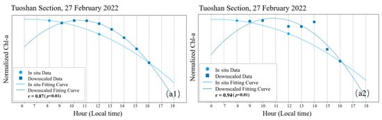
Figure 8.
Comparison of daily trends of measured and downscaled Chl-a concentrations (normalized to 0–1 range) on 27 February 2022. (a1) RTAD method (a2) TWD method.
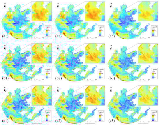
Figure 9.
Chl-a concentration distribution on 27 February 2022; 1–3 are 9:00, 13:00, and 16:00 local time, respectively; (a1–a3) COMS-1 GOCI inversion data after correction; (b1–b3) data after downscaling using the RTAD method; (c1–c3) data downscaled using TWD method.
Figure 8 demonstrates that the Chl-a concentration on that day showed an overall trend of first increasing and then decreasing. Compared with the measured data at Tuoshan Station in Northwest Taihu Lake, the daily variation trend of Chl-a obtained using the RTAD and TWD downscaling methods was consistent with the measured data. The fitting coefficients of the trends reached 0.87 and 0.94, respectively, indicating that the downscaling results on that day were consistent with the actual situation.
As can be seen in Figure 9, during the period of 9:00–16:00 local time on February 27, the downscaled data successfully captured the spatial distribution characteristics and temporal variation trends of Chl-a, which was consistent with the measured results.
In terms of spatial distribution characteristics, the original COMS-1 GOCI inversion data were consistent with the Chl-a data obtained using the two downscaling methods. The main high-value areas were concentrated along the southwestern coast of Meiliang Bay and the southern lakeshore area. However, compared with the original COMS-1 GOCI inversion data, the downscaling results showed more spatial distribution details of Chl-a. For example, a regional Chl-a concentration of 38.44 μg/L was detected on the northwest coast, whereas the data before downscaling failed to observe this high-value area. The capture of this detail further confirms the importance of the high spatial resolution in algal bloom monitoring.
In terms of the time change trends, the downscaling results were highly consistent with the original COMS-1 GOCI inversion data. Taking the northwest region with obvious changes as an example, the average high value of Chl-a concentration that day increased from 33.36 μg/L at 9:00 to 37.04 μg/L at 13:00 and then gradually declined to 27.64 μg/L at 16:00 after reaching the peak; the overall trend exhibited a slight increase at first and then a sharp decrease. This trend was successfully captured in the hourly scale results after downscaling and was inferred to be the reduction period after the algal bloom outbreak.
In summary, the downscaled Chl-a concentration retains the daily variation trend of the original GOCI inversion data, shows more spatial details, and significantly improves the accuracy of the data. Through the tracking of this algal bloom event, it is once again confirmed that the downscaling work of this study is feasible and effective in practical applications. High-frequency and high-precision Chl-a monitoring has application value in supporting emergency response decisions, pollutant tracking and tracing, and quantitative evaluation of ecological restoration. It also reveals the important practical significance of high-frequency Chl-a monitoring in water environment management and cyanobacteria bloom early warning.
4.5. Temporal and Spatial Distribution Characteristics of Chlorophyll-a Concentration in Taihu Lake
Based on the downscaling results, the revealed spatiotemporal patterns of the Chl-a concentration in Taihu Lake were obtained. In terms of the time scale, the variation characteristics at three levels, namely, interannual, seasonal, and daily scales, were shown. Among them, interannual variation was derived from annual averages (2019–2023), seasonal variation in the triennial averages of different seasons (2019–2023), and daily scale variation from Chl-a concentration data within 7 h from 9:00 to 16:00 on a day when algal blooms occurred and the daily trend was obvious.
As can be seen in Figure 10, the high-value areas of Chl-a in Taihu Lake are mainly distributed in the nearshore and estuaries on the west and north sides, mainly including the Taige Canal on the north bank, Changxing Port on the west bank, and Dongshaoxi and Xishaoxi on the southwest bank, whereas the low-value areas are mainly distributed in the open waters in the center of the lake and the eastern region. The multi-year average Chl-a concentration exhibited a persistent northwest–southeast gradient, which was high in the northwest and low in the southeast. Over the past five years, the spatial distribution range and concentration level of Chl-a generally increased and then decreased. The annual average Chl-a concentration was 3.76 µg/L in 2019 and rose to 3.87 µg/L in 2020. It began to decline thereafter and reached 1.85 µg/L in 2023, which was only half of that in 2019. Simultaneously, the high-value area in the north was suppressed well. This interannual variation trend was mainly related to the water resource management of the relevant departments of Taihu Lake.
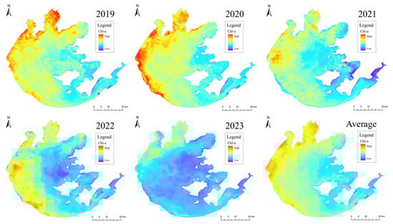
Figure 10.
Spatial distribution and interannual variation of Chl-a concentration in Taihu Lake.
As shown in Figure 11, Chl-a showed significant changes in the different seasons. The overall high-value range in spring was small and the concentration level was low, mainly distributed on the northwest coast, with an average concentration of 2.59 μg/L; summer was the season with the most severe Chl-a outbreaks, in Zhushan Lake, Meiliang Bay, and Gonghu Bay in the north, which were key outbreak areas. In severe cases, it covered the entire lake, and the average concentration over many years can reach 4.91 μg/L. In autumn, the Chl-a concentration declined, but there were still high-value areas in the Dapukou area in the west, with the average concentration reaching 3.57 μg/L; in winter, it is the season with the lowest Chl-a concentration level. There was no obvious high-value area, and the average concentration was 1.65 μg/L.
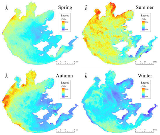
Figure 11.
Spatial distribution and seasonal variation characteristics of Chl-a concentration in Taihu Lake.
Seasonal differences were mainly related to light and temperature. In summer, rising water temperatures and long sunshine hours can accelerate the photosynthesis of phytoplankton, promote an increase in the number of algae, and maintain a high concentration of Chl-a. At the same time, summer was usually accompanied by an increase in rainfall and runoff, which brought a large amount of N, P, and other substances into the lake, providing a rich source of nutrients for algae [44,45]. In winter, the temperature was lower and the water temperature dropped, which significantly inhibited photosynthesis and the growth of phytoplankton [46], leading to a decrease in the Chl a concentration.
On a daily scale (Figure 12), the Chl-a concentration changed regularly and dynamically at different times. Within a single day, the spatial distribution pattern of Chl-a was basically stable, and the changes were mainly manifested in that the concentration in the high-value area in the morning (9:00–10:00) was low, within the range of 5–15 μg/L, and at the same time, it diffused over time with 1–2 high-value points as the source. At noon (13:00–14:00), owing to the increase in temperature and enhanced light, Chl-a reached its maximum value in both range and concentration, and sometimes, multiple high-value points appeared in the northern, eastern, and western coastal areas, with concentrations reaching more than 30 μg/L; in the afternoon (15:00–16:00), the concentration of Chl-a gradually decreased and returned to normal levels, and the range of the high-value area shrank toward the coast. However, unlike the relatively stable patterns between years and seasons, the daily variation trend of Chl-a was affected not only by temperature but also by multiple factors such as nutrient levels on different dates, water mixing conditions, and human activities. It exhibited context-dependent variability. The purpose of this study’s temporal downscaling was to capture such diverse and complex changes.
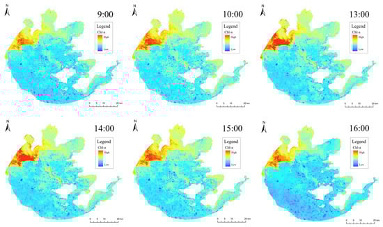
Figure 12.
Spatial distribution and daily variation characteristics of Chl-a concentration in Taihu Lake.
Based on the above characteristics, it can be considered that the spatial distribution pattern of Chl-a in nearshore and estuary areas is mainly related to the discharge of coastal agricultural runoff, domestic sewage, and industrial wastewater, which is consistent with the conclusions of many previous studies [47,48,49,50]. The specific reason is that the large-scale discharge of sewage has led to a significant increase in the content of nutrients such as nitrogen and phosphorus in the lake water, providing conditions for the reproduction of phytoplankton. At the same time, differences in hydrodynamic conditions made it easier for nutrient salt to accumulate in estuary areas, leading to an increase in Chl-a concentration in these areas [51]. The temporal variation characteristics of the Chl-a concentration were the result of the joint action of water temperature, light, and other natural environmental factors. During periods of insufficient light and low temperatures, algal photosynthesis was weak. When the light intensity increased, the temperature also increased, prompting algae to reproduce and accumulate in large numbers, showing the characteristics of a concentrated distribution of high Chl-a concentration.
The above findings were consistent with the results of Xue et al. and Ma et al. [51,52] on lake algae, further confirming the advantages of high-precision remote sensing data in dynamically monitoring changes in lake water quality.
5. Discussion
5.1. Pre-Correction of Chlorophyll-a Inversion Data
It was necessary to correct inversion data before downscaling, which was reflected in the following aspects:
First, there were discrepancies across technical specifications such as resolution, sensor design, orbit characteristics, observation geometry, and processing methods between the two data sources, which caused objective systematic biases, as shown in Table 2 above.
For data preprocessing, Yang et al. [53] proposed that the atmospheric correction process of ocean satellites would fail for inland turbid water bodies when using COMS-1 GOCI data to invert the Chl-a concentration in Hangzhou Bay in 2020. Zhang et al. [54] further noted that the opacity of high-concentration suspended matter (TSM) would interfere with the spectral measurement of Chl-a concentration and thus affect the inversion accuracy of Chl-a concentration when using COMS-1 GOCI data to invert Chl-a in the Yellow River estuary. Zeng et al. [55] found that the 6S model would slightly over-correct when processing COMS-1 GOCI data using COMS-1 GOCI . In summary, our study may have introduced data errors into the atmospheric correction process of COMS-1 GOCI, which reduced the data accuracy compared with the official atmospheric correction process used in the Sentinel-2 L2A product.
In terms of inversion algorithms, the COMS-1 GOCI had fewer band settings, limiting the application of high-precision multiband models. In addition, owing to differences in water body components and their bio-optical properties, there was a large variability in the optimal band position of the inversion factor and the inversion model parameters, which greatly reduced the universality of the multiband Chl-a inversion model [56]. The COMS-1 GOCI three-band inversion model used in this study was constructed based on a sample dataset collected from 17 inland lakes in China from 2013 to 2020 [37], and the Sentinel-2 MSI inversion model was constructed based on an actual sampling dataset at 22 stations in the Taihu Lake area, according to the waterway and actual hydrological conditions [57]. Compared to COMS-1 GOCI, the Sentinel-2 MSI inversion model was more suitable for Taihu Lake.
Satellite-derived versus in situ comparisons revealed that the inverted COMS-1 GOCI Chl-a concentrations were generally higher, whereas those of Sentinel-2 MSI were normal, which also confirms the above point of view. If this systematic bias were not corrected, it would significantly affect the accuracy of subsequent temporal downscaling results.
Secondly, from the downscaling method perspective, temporal downscaling requires comparable data from COMS-1 GOCI and Sentinel-2 MSI. Large differences between these datasets can introduce errors during data fusion, reducing the reliability of the final product. Thus, the correction step is crucial for ensuring result quality.
Judging from the final actual results, the correlation between the COMS-1 GOCI data corrected by the random forest model and the Sentinel-2 MSI data was greatly improved, with the determination coefficient R2 reaching a maximum of 0.93, while still maintaining the original spatiotemporal distribution characteristics, reflecting the necessity and correctness of the correction process.
This study adopted an important assumption when correcting the COMS-1 GOCI data: the time trend of the corrected COMS-1 GOCI data was still reliable. The rationality of this assumption was based on the following aspects:
Firstly, from a methodological point of view, this study used a machine learning model for correction, which mainly focused on the adjustment of numerical ranges rather than the reconstruction of time-series patterns. The training process of the model was based on feature mapping of the corresponding spatial points rather than the time series reconstruction, which ensured that the time-varying information contained in the original data was not significantly disturbed.
Secondly, the introduction of the time difference characteristics () in the correction process and the spatial smoothing of the Gaussian filtering method not only enable the model to retain the influence of the observation time on the inversion results but also indirectly enhance the stability of the time series, which helps to suppress abnormal fluctuations and make the assumption of time trend more reliable.
However, this assumption had several limitations. The random forest correction method itself did not focus on the autocorrelation of the time series and may ignore complex time dependencies. If multiple consecutive days of data were processed, the correlation between the different dates may be weakened. Although the non-parametric characteristics of the random forest model provided better nonlinear fitting capabilities, they may also overfit spatial features in some cases, thereby affecting the reliability of time trends.
In practical applications, especially in lakes with more complex water types (such as the coexistence of bays and open waters, many rivers entering the lake, and complex ecological composition), or under certain special meteorological conditions (such as severe convective weather), the daily variation pattern of Chl-a may be affected by many factors, and the actual temporal variation of Chl-a showed a large mutation. At this time, assumptions based on the temporal variation trend may not accurately reflect the actual change process.
5.2. Comparison of RTAD and TWD Downscaling Methods
In the RTAD method, since constructed trend equations are temporally continuous, extended data beyond baseline timepoints t can be obtained. However, the construction of the trend equation is limited by the time attribute of the basic data, and the downscaling results are heavily affected by the data in the time period before and after the target time point. The independence of the model is low. When there are abnormal changes in some interval values, it will have a certain impact on the result values of the remaining data, making it difficult to capture abnormal value changes, thereby affecting the overall data accuracy. In terms of the statistical data of many years (Figure 5), when the Chl-a concentration distribution is close to a random trend as a whole, the regression trend fitting model is not able to obtain trend changes, which leads to a decrease in the overall fitting R2.
The TWD method uses the ratio between the base time and target time data as the time weight to obtain trend changes and extrapolates Chl-a concentration data of Sentinel-2 MSI at different times according to the weight. Compared with the RTAD method, the TWD input data correspond to the time of the output result one by one, and data outside the basic data time point cannot be obtained. However, the model trend acquisition only depends on the relevant two-time data. The method has high independence and is not affected by the data of non-target time in the time period. It has a strong ability to capture abnormal value changes.
The downscaling results obtained using the two methods were verified for accuracy (Table 2). Table 2 indicates that the overall fitting rate of the TWD method was higher than that of the RTAD method. In the correctly fitted part, the RTAD method had a higher proportion of good and high fit, and the highest fitting coefficient was larger, reaching 0.98.
The difference between the two methods was related to the mechanism of each method. The TWD method had strong independence owing to the calculation of time weight at a single moment, and the overall effect was not easily disturbed by abnormal data. It performed better when downscaling data with complex trend changes; therefore, the overall fitting rate was higher. Although the RTAD method reduced the ability to capture details in the process of fitting daily changes by constructing a trend equation, it produced good results when processing data series with clear trends. It can be considered that the more regular the trend of the Chl-a change, the higher the accuracy of the downscaling results of the RTAD method. Therefore, in the fitting part, the RTAD method exhibited a higher degree of fitting.
In general, the results of the two downscaling methods performed well, and the data results were reasonable; however, some results were inconsistent with the site data. When analyzing the entire research process, this inconsistency may be caused by the accumulation of errors in multiple links:
First, this study referred to the inversion models developed by scholars based on different datasets and research periods, which cannot be fully applied to the data inversion of this study, especially in the high-turbidity water area of Taihu Lake. The accuracy of Chl-a inversion is affected by the scattering and absorption of total suspended matter (TSM), and colored dissolved organic matter (CDOM) also masks the characteristic spectrum of Chl-a through strong absorption in certain bands. Although this factor has been taken into account during the construction of the inversion model and the influence of TSM and CDOM has been reduced as much as possible, this interference cannot be completely eliminated. The R2 test of the inversion model is 0.82 and 0.78, which has a certain impact on the accuracy of the data. Secondly, the random forest correction model used in the study weakens the temporal continuity characteristics of the data to a certain extent based on the pixel processing method. The subsequent addition of Gaussian filtering may also blur local changes with ecological significance while reducing spatial noise.
The biggest reason for the inconsistency between the model and the actual trend was that both downscaling methods were based on simplified assumptions and did not consider the influence of environmental factors such as hydrodynamic processes, meteorology, and climate. Under certain circumstances, they may not be able to fully express the complexity of the dynamic changes in Chl-a. In current research, downscaling methods can be divided into two parts: dynamic downscaling and statistical downscaling. The dynamic downscaling model was complex, the data volume was large, and it was difficult to transfer. The statistical downscaling model was relatively simple [58]. The downscaling methods used in this study were all statistical. Compared with other current statistical downscaling techniques, including quantile mapping (QM) [59], tectonic simulation (CA) [60], spatial decomposition bias correction (BCSD) [61], and more complex deep learning algorithms [62,63,64,65,66,67], the downscaling model constructed in this study was relatively simple and did not introduce environmental factors as model parameters. Deng et al. [68] collected field monitoring data in Meiliang Bay and concluded that the key driving factors affecting the Chl-a concentration included the water temperature, light, and simulation time, which were closely related to hydrodynamic processes and meteorological conditions. Shi et al. [69] also emphasized the impact of meteorological conditions on the Chl-a concentration in Taihu Lake, pointing out that high air temperature and low air pressure levels were closely related to the outbreak of cyanobacteria and that the degree of influence of air temperature on cyanobacteria growth varies in different areas, such as Meiliang Bay and Gonghu Bay. The lack of model-related environmental parameters might be an important reason for the poor performance of this method during rapid environmental changes or concentrated outbreaks of algal blooms.
In addition to the limitations of the research methods, the complex ecological environment of the region itself also increases the possibility of sudden changes in the Chl-a concentration. Against the backdrop of global warming, the frequency and intensity of extreme weather events in coastal areas have also increased significantly, and these events have a significant impact on the entire ecosystem around Taihu Lake. Taihu Lake has a large area and frequent water exchanges with the outside world. Its water bodies are susceptible to environmental factors such as complex wind-driven circulation and input from surrounding rivers. Under extreme conditions, these factors may lead to sudden changes in Chl-a [70]. In this process, biological processes such as the vertical migration of algae and their specific response to environmental conditions also make the temporal variation pattern more complex [71]. Under such special conditions, the response mechanism of Chl-a concentration to extreme environmental stress may exceed the training scope of the research model, increasing downscaling errors.
In summary, the Chl-a concentration downscaling method proposed in this study had errors accumulating in multiple links, which may cause uncertainty in the final results. Nevertheless, this study achieved an effective improvement in the spatiotemporal resolution of traditional remote sensing data, and the method had a certain degree of credibility.
5.3. Generalizability of Spatiotemporal Downscaling Model
This study selected COMS-1 GOCI and Sentinel-2 MSI data for downscaling, but the application scope of this method was not limited to these two specific data sources. As long as the data meet the characteristics of complementary temporal and spatial resolutions, this method can be applied for downscaling, for example, the combination of MODIS and Landsat, VIIRS, and Gaofen series. The flexibility of this data source allows different studies to select the most appropriate data combination according to the actual situation of the region and data availability, providing a reliable data foundation for the subsequent downscaling.
In terms of the practical application of the model, the efficiency of information acquisition and decision making was particularly important for water quality monitoring (especially large-scale, real-time monitoring). Therefore, improving the computational efficiency of the model and reducing the computational cost was important for ensuring its wide application in actual monitoring. The downscaling model established in this study based on statistical methods was relatively simple, had a low demand for computing resources, and could quickly obtain downscaling results, providing data support for subsequent analyses.
In addition to Chl-a, the method proposed in this study can be extended to downscale other water quality and meteorological parameters, especially those with obvious daily variation characteristics. In water quality monitoring, it can also be applied to other water quality indicators, such as turbidity, dissolved oxygen (DO), suspended matter concentration, temperature, and pH, to provide more accurate spatiotemporal data for dynamic monitoring of water quality or atmospheric changes.
5.4. Limitations of Spatiotemporal Downscaling Model and Future Work
This study used Sentinel-2 MSI and COMS-1 GOCI to invert Chl-a data for data downscaling. The source data were mature and had a high resolution, which met the monitoring needs of Chl-a in both time and space. However, due to systematic differences in data sources, coupled with the limitations of preprocessing and inversion methods, there were deviations in the inverted data. This study used a precorrection model to improve it, but this deviation could not be completely eliminated.
The random forest model correction method used in this study also has some limitations, mainly reflected in the fact that the correction process is based on the independent processing of pixels, which may cause spatial discontinuity problems due to the lack of consideration of the spatial correlation between adjacent pixels. Additionally, the correction process may introduce new uncertainties, which were transmitted to the subsequent downscaling process and affect the accuracy of the final data.
In the process of data verification, this study compared the daily variation trend of the Chl-a inversion value after downscaling with the measured Chl-a concentration value. The high fitting coefficient and significance became a strong indication of the feasibility of the research method. However, since the inversion model used was constructed under a dataset with a lower time resolution, the influence of fluorescence changes caused by the diurnal cycle at the sub-daily scale on the Chl-a inversion results and the measured results was not considered, which limited the data accuracy of the study to validate the downscaling results.
The downscaling model constructed in this study was relatively simple and relied only on the Chl-a inversion results, without involving relevant hydrological and meteorological parameters, which further limited the ability of the model to capture the distribution and changes in Chl-a.
In view of the current limitations of the research, the team will further optimize the following aspects in future research:
- We will introduce satellite data with a higher temporal resolution, such as Japan’s Himawari-9 and China’s Fengyun-4 series, to improve the downscaling effect and quickly capture the dynamic changes in elements.
- We plan to construct an inversion model suitable for the study area based on the water characteristics of different lakes, with a particular focus on developing differentiated inversion strategies according to water body zoning and the impact of non-Chl-a factors on the diurnal variation of fluorescence.
- We will enhance the overall ability of the model to capture trend changes by considering the introduction of more complex machine learning algorithms, given that the model constructed in this study was relatively simple to apply compared to current downscaling methods.
- We intend to expand the input parameters of the model by including hydrological data such as hydrodynamic models. This will improve the physical mechanisms and interpretability of the model, enhance its generalization ability, and lay the foundation for further research on constructing an early warning system for harmful cyanobacterial blooms.
6. Conclusions
Based on high-temporal-resolution COMS-1 GOCI and high-spatial-resolution Sentinel-2 MSI Chl-a inversion data, a spatiotemporal downscaling model based on the machine learning pre-correction method was successfully constructed. The model effectively reduced the data deviation caused by a series of tasks before downscaling through the adaptive bias pre-correction method of the random forest model and increased the R2 of the two data sources to 0.93 while retaining the temporal trend of GOCI. The corrected data were used to perform downscaling based on the RTAD and TWD methods, and the temporal resolution of the Sentinel-2 MSI Chl-a data was successfully increased from 5 d to 1 h. Verified by the measured data, the overall fit of the model was ideal, and the best fit was 0.98. The credibility of the inversion results was further proven by combining the actual cyanobacteria bloom events in Taihu Lake.
After comparative analysis, the overall fitting rate of the TWD method was higher than that of the RTAD method, which had strong independence and was not easily affected by data from other time points. In terms of the already fitted parts, the RTAD method had a higher proportion of good fit and high fit, which can better capture daily trend changes. The downscaling results were more accurate in the data interval, with more obvious trends. For wide water, where the Chl-a value exhibits regular variations, the RTAD method can be used. The TWD method is more suitable for areas such as lakes and bays, where the changing trend is difficult to capture.
The downscaling method constructed in this study successfully obtained high-precision Chl-a monitoring data with a temporal resolution of 1 h and a spatial resolution of 10 m, effectively captured the trend of intraday Chl-a changes, improved data accuracy, and helped in related water environment management and cyanobacteria bloom early warning monitoring. This method can be applied to the downscaling of water quality parameters, such as Chl-a in other waters, has great promotion potential, meets the needs of refined water body monitoring, and provides data support for water environment management.
Author Contributions
Conceptualization, C.W., M.X., L.L., S.H. and C.L.; methodology, C.W., M.X. and L.L.; software, C.W., M.X. and L.L.; validation, C.W. and M.X.; formal analysis, C.W. and M.X.; investigation, L.L.; data curation, C.W., M.X. and L.L.; writing—original draft preparation, C.W., M.X. and L.L.; writing—review and editing, S.H., C.L. and H.D.; visualization, C.W. and M.X.; supervision, S.H. and H.D.; project administration, C.W. All authors have read and agreed to the published version of the manuscript.
Funding
This research was financially supported by the 2024 Hubei National College Students Innovation and Entrepreneurship Training Program (project No. 202410497041); 2024 Ningbo Municipal Public Welfare Research Plan Project, grant number 2024S008.
Data Availability Statement
The raw data required to reproduce the study results are included in this article.
Acknowledgments
We thank Heng Dong, Sicong He and Chichang Luo for their suggested comments for the manuscript.
Conflicts of Interest
The authors declare that they have no known competing financial interests or personal relationships that could appear to influence the work reported in this article.
References
- Zhang, Y.; Li, M.; Dong, J.; Yang, H.; Van Zwieten, L.; Lu, H.; Alshameri, A.; Zhan, Z.; Chen, X.; Jiang, X.; et al. A Critical Review of Methods for Analyzing Freshwater Eutrophication. Water 2021, 13, 225. [Google Scholar] [CrossRef]
- Suresh, K.; Tang, T.; van Vliet, M.; Bierkens, M.; Strokal, M.; Sorger-Domenigg, F.; Wada, Y. Recent advancement in water quality indicators for eutrophication in global freshwater lakes. Environ. Res. Lett. 2023, 18, 063004. [Google Scholar] [CrossRef]
- Chen, C.; Chen, Q.; Yao, S.; Mengnan, H.; Zhang, J.; Li, G.; Lin, Y. Combining physical-based model and machine learning to forecast chlorophyll-a concentration in freshwater lakes. Sci. Total Environ. 2023, 907, 168097. [Google Scholar] [CrossRef]
- Cao, Z.; Ma, R.; Melack, J.; Duan, H.; Liu, M.; Kutser, T.; Xue, K.; Shen, M.; Qi, T.; Yuan, H. Landsat observations of chlorophyll-a variations in Lake Taihu from 1984 to 2019. Int. J. Appl. Earth Obs. 2022, 106, 102642. [Google Scholar] [CrossRef]
- Makwinja, R.; Inagaki, Y.; Tesfamichael, S.; Curtis, C. Novel methods for monitoring low chlorophyll-a concentrations in the large, oligotrophic Lake Malawi/Nyasa/Niassa. J. Environ. Manag. 2024, 364, 121462. [Google Scholar] [CrossRef]
- Qin, B.; Li, W.; Zhu, G.; Zhang, Y.; Wu, T.; Gao, G. Cyanobacterial bloom management through integrated monitoring and forecasting in large shallow eutrophic Lake Taihu (China). J. Hazard. Mater. 2015, 287, 356–363. [Google Scholar] [CrossRef]
- Yang, H.; Kong, J.; Hu, H.; Du, Y.; Gao, M.; Chen, F. A Review of Remote Sensing for Water Quality Retrieval: Progress and Challenges. Remote Sens. 2022, 14, 1770. [Google Scholar] [CrossRef]
- Buma, W.; Lee, S. Evaluation of Sentinel-2 and Landsat 8 Images for Estimating Chlorophyll-a Concentrations in Lake Chad, Africa. Remote Sens. 2020, 12, 2437. [Google Scholar] [CrossRef]
- Kravitz, J.; Matthews, M.; Bernard, S.; Griffith, D. Application of Sentinel 3 OLCI for chl-a retrieval over small inland water targets: Successes and challenges. Remote Sens. Environ. 2019, 237, 111562. [Google Scholar] [CrossRef]
- Li, H.; He, X.; Shanmugam, P.; Bai, Y.; Wang, D.; Li, T.; Gong, F. Assessing and Improving the Accuracy of Visible Infrared Imaging Radiometer Suite Ocean Color Products in Environments with High Solar Zenith Angles. Remote Sens. 2024, 16, 339. [Google Scholar] [CrossRef]
- Ogashawara, I. The Use of Sentinel-3 Imagery to Monitor Cyanobacterial Blooms. Environments 2019, 6, 60. [Google Scholar] [CrossRef]
- Tilstone, G.; Pardo, S.; Dall’Olmo, G.; Brewin, B.; Nencioli, F.; Dessailly, D.; Kwiatkowska, E.; Casal, T.; Donlon, C. Performance of Ocean Colour Chlorophyll a algorithms for Sentinel-3 OLCI, MODIS-Aqua and Suomi-VIIRS in open-ocean waters of the Atlantic. Remote Sens. Environ. 2021, 260, 112444. [Google Scholar] [CrossRef]
- Fu, Y.; Xu, S.; Zhang, C.; Sun, Y. Spatial downscaling of MODIS Chlorophyll-a using Landsat 8 images for complex coastal water monitoring. Estuar. Coast. Shelf Sci. 2018, 209, 149–159. [Google Scholar] [CrossRef]
- Jöhnk, K.D.; Huisman, J.; Sharples, J.; Sommeijer, B.; Visser, P.M.; Stroom, J.M. Summer heatwaves promote blooms of harmful cyanobacteria. Glob. Change Biol. 2008, 14, 495–512. [Google Scholar] [CrossRef]
- Lekki, J.; Deutsch, E.; Sayers, M.; Bosse, K.; Anderson, R.; Tokars, R.; Sawtell, R. Determining remote sensing spatial resolution requirements for the monitoring of harmful algal blooms in the Great Lakes. J. Great Lakes Res. 2019, 45, 434–443. [Google Scholar] [CrossRef]
- Shi, K.; Zhang, Y.; Qin, B.; Zhou, B. Remote sensing of cyanobacterial blooms in inland waters: Present knowledge and future challenges. Sci. Bull. 2019, 64, 1540–1556. [Google Scholar] [CrossRef]
- Park, M.; Lee, S.; Ahn, J.; Lee, S.; Choi, J.; Ryu, J. Decadal Measurements of the First Geostationary Ocean Color Satellite (GOCI) Compared with MODIS and VIIRS Data. Remote Sens. 2021, 14, 72. [Google Scholar] [CrossRef]
- Liu, X.; Wang, M. Filling the gaps of missing data in the merged VIIRS SNPP/NOAA-20 ocean color product using the DINEOF method. Remote Sens. 2019, 11, 178. [Google Scholar] [CrossRef]
- Bonansea, M.; Rodriguez, C.; Pinotti, L. Assessing the potential of integrating Landsat sensors for estimating chlorophyll-a concentration in a reservoir. Hydrol. Res. 2017, 49, 1608–1617. [Google Scholar] [CrossRef]
- Zhao, D.; Huang, J.; Li, Z.; Yu, G.; Shen, H. Dynamic monitoring and analysis of chlorophyll-a concentrations in global lakes using Sentinel-2 images in Google Earth Engine. Sci. Total Environ. 2024, 912, 169152. [Google Scholar] [CrossRef]
- Xu, Y.; Chen, J.; Yang, Q.; Jiang, X.; Fu, Y.; Pan, D. Trend of harmful algal bloom dynamics from GOCI observed diurnal variation of chlorophyll a off Southeast coast of China. Front. Mar. Sci. 2024, 11, 1357669. [Google Scholar] [CrossRef]
- Bai, J.; Cui, Q.; Zhang, W.; Meng, L. An approach for downscaling SMAP soil moisture by combining Sentinel-1 SAR and MODIS data. Remote Sens. 2019, 11, 2736. [Google Scholar] [CrossRef]
- Chu, J.; Su, X.; Zhang, T.; Lei, Y.; Jiang, T.; Wu, H.; Wang, Q. Comparison of three spatial downscaling concepts of GRACE data using random forest model. J. Lake Sci. 2024, 36, 951–962. (In Chinese) [Google Scholar] [CrossRef]
- Nomura, R.; Oki, K. Downscaling of MODIS NDVI by Using a Convolutional Neural Network-Based Model with Higher Resolution SAR Data. Remote Sens. 2021, 13, 732. [Google Scholar] [CrossRef]
- Zhang, S.; Liu, N.; Luo, M.; Jiang, T.; Chan, T.; Yau, C.; Sun, Y. Downscaling Sentinel-3 Chlorophyll-a Concentration for Inland Lakes Based on Multivariate Analysis and Gradient Boosting Decision Trees Regression. IEEE J. Sel. Top. Appl. Earth Obs. Remote Sens. 2023, 16, 7850–7865. [Google Scholar] [CrossRef]
- He, Q.; Chen, C.; Wang, Y.; Sun, Y.; Liu, Y.; Hu, B. Fusion Method for Multi-Source Remote Sensing Daily Precipitation Data: Random Forest Model Considering Spatial Autocorrelation. J. Geo-Inf. Sci. 2024, 26, 1517–1530. [Google Scholar] [CrossRef]
- Michel, A.; Sharma, V.; Lehning, M.; Huwald, H. Climate change scenarios at hourly time-step over Switzerland from an enhanced temporal downscaling approach. Int. J. Climatol. 2021, 41, 3503–3522. [Google Scholar] [CrossRef]
- Qin, B.; Paerl, H.; Brookes, J.; Liu, J.; Jeppesen, E.; Zhu, G.; Zhang, Y.; Xu, H.; Shi, K.; Deng, J. Why Lake Taihu continues to be plagued with cyanobacterial blooms through 10 years (2007–2017) efforts. Sci. Bull. 2019, 64, 354–356. [Google Scholar] [CrossRef]
- Le, C.; Zha, Y.; Li, Y.; Sun, D.; Lu, H.; Yin, B. Eutrophication of Lake Waters in China: Cost, Causes, and Control. Environ. Manag. 2010, 45, 662–668. [Google Scholar] [CrossRef]
- Qin, B.; Xu, P.; Wu, Q.; Luo, L.; Zhang, Y. Environmental issues of Lake Taihu, China. Hydrobiologia 2007, 581, 3–14. [Google Scholar] [CrossRef]
- Hu, H. Remote Sensing Monitoring and Early Warning of Algal Bloom in Chaohu Lake Based on Deep Learning. Master’s Thesis, Anhui University, Hefei, China, 2022. [Google Scholar]
- Bingchuan, Z.; Kai, Y.; Junze, S.; Wei, W.; Liang, Y. Retrieval of Chlorophyll-a Concentration and Remote Sensing Monitoring of Cyanobacterial Blooms in Lake Taihu Based on GOCI Data. Environ. Pollut. Its Prev. 2020, 42, 1021–1025. [Google Scholar] [CrossRef]
- Guo, Y.; Wei, X.; Huang, Z.; Li, H.; Ma, R.; Cao, Z.; Shen, M.; Xue, K. Retrievals of Chlorophyll-a from GOCI and GOCI-II Data in Optically Complex Lakes. Remote Sens. 2023, 15, 4886. [Google Scholar] [CrossRef]
- Bai, L.; Gao, J.; Sun, Z.; Tian, S. Monitoring Water Transparency in Shallow and Eutrophic Lake Waters Based on GOCI Observations. Remote Sens. 2020, 12, 163. [Google Scholar] [CrossRef]
- Huang, C.; Shi, K.; Yang, H.; Li, Y.; Zhu, A.; Sun, D.; Xu, L.; Zou, J.; Chen, X. Satellite observation of hourly dynamic characteristics of algae with Geostationary Ocean Color Imager (GOCI) data in Lake Taihu. Remote Sens. Environ. 2015, 159, 278–287. [Google Scholar] [CrossRef]
- Cao, H.; Han, L. Hourly remote sensing monitoring of harmful algal blooms (HABs) in Taihu Lake based on GOCI images. Environ. Sci. Pollut. Res. 2021, 28, 35958–35970. [Google Scholar] [CrossRef]
- Guo, Y.; Du, C.; Li, Y.; Chen, W.; Shi, L.; Ji, G. An Expanded Three Band Model to Monitor Inland Optically Complex Water Using Geostationary Ocean Color Imager (GOCI). Front. Remote Sens. 2022, 3, 803884. [Google Scholar] [CrossRef]
- Dall Olmo, G.; Gitelson, A.A. Effect of bio-optical parameter variability on the remote estimation of chlorophyll-a concentration in turbid productive waters: Experimental results. Appl. Opt. 2005, 44, 412–422. [Google Scholar] [CrossRef]
- Wang, Y. Research and Application of the Extraction Method of Cyanobacteria Bloom in Taihu Lake based on Sentinel-2A Images. Master’s Thesis, China University of Geosciences, Beijing, China, 2020. [Google Scholar]
- Salls, W.; Schaeffer, B.; Pahlevan, N.; Coffer, M.; Seegers, B.; Werdell, J.; Ferriby, H.; Stumpf, R.; Binding, C.; Keith, D. Expanding the Application of Sentinel-2 Chlorophyll Monitoring across United States Lakes. Remote Sens. 2024, 16, 1977. [Google Scholar] [CrossRef]
- Huang, L.; Fang, H.; He, G.; Jiang, H.; Wang, C. Effects of internal loading on phosphorus distribution in the Taihu Lake driven by wind waves and lake currents. Environ. Pollut. 2016, 219, 760–773. [Google Scholar] [CrossRef]
- Qin, B.; Hu, W.; Chen, W.; Fan, C.; Ji, J.; Chen, Y.; Gao, X.; Yang, L.; Gao, G.; Huang, W.; et al. Studies on the Hydrodynamic Processes and Related Factors in Meiliang Bay, Northern Taihu Lake, China. J. Lake Sci. 2000, 12, 327–334. [Google Scholar] [CrossRef]
- Song, T.; Zhang, J.; Li, X.; Zhu, J.; Hu, J. Cyanobacterial blooms in yellow. J. Lake Sci. 2022, 34, 1384–1391. [Google Scholar] [CrossRef]
- Liu, X.; Liu, H.; Chen, H.; Liu, Y.; Xu, Z.; Cao, X.; Ma, L.; Pan, B.; Wang, L. Spatiotemporal distribution and prediction of chlorophyll-a in Ulansuhai lake from an arid area of China. Front. Environ. Sci. 2023, 11, 1045464. [Google Scholar] [CrossRef]
- Kim, W.; Moon, J.; Park, Y.; Ishizaka, J. Evaluation of chlorophyll retrievals from Geostationary Ocean Color Imager (GOCI) for the North-East Asian region. Remote Sens. Environ. 2016, 184, 482–495. [Google Scholar] [CrossRef]
- Armonies, W.; Herre, E.; Sturm, M. Effects of the severe winter 1995/96 on the benthic macrofauna of the Wadden Sea and the coastal North Sea near the island of Sylt. Helgol. Mar. Res. 2001, 55, 170–175. [Google Scholar] [CrossRef]
- Li, J.; Yan, D.; Qi, L.; Shi, D.; Luan, Z. Temporal and spatial variation characteristics and driving mechanisms of vegetation in Taihu Lake wetlands. J. Beijing Norm. Univ. 2021, 57, 94–103. [Google Scholar]
- Wu, Z.; Xu, Z.; Zeng, J.; Liu, X. Analysis on the spatiotemporal characteristics of chlorophyll-a concentration in Chinese lakes over the past 40 years. Ocean. Lakes 2024, 55, 347–362. [Google Scholar]
- Zhao, Y.; Lu, X.; Ma, Y.; Li, Z.; Liu, Y.; Fan, Y. Characteristics of benthic diatom communities and water environment health assessment in the Ash River Basin. Ocean. Lakes 2020, 51, 307–317. [Google Scholar]
- Huang, H.; Wang, W.; Lv, J.; Liu, Q.; Liu, X.; Xie, S.; Wang, F.; Feng, J. Relationship between Chlorophyll a and Environmental Factors in Lakes Based on the Random Forest Algorithm. Water 2022, 14, 3128. [Google Scholar] [CrossRef]
- Ma, R.; Kong, F.; Duan, H.; Zhang, S.; Kong, W.; Hao, J. Spatio-temporal distribution of cyanobacteria blooms based on satellite imageries in Lake Taihu, China. J. Lake Sci. 2008, 20, 687–694. [Google Scholar] [CrossRef]
- Xue, K.; Ma, R.; Cao, Z.; Shen, M.; Hu, M.; Xiong, J. Monitoring fractional floating algae cover over eutrophic lakes using multisensor satellite images: MODIS, VIIRS, GOCI, and OLCI. IEEE Trans. Geosci. Remote. Sens. 2022, 60, 1–15. [Google Scholar] [CrossRef]
- Yang, Y.; He, S.; Gu, Y.; Zhu, C.; Wang, L.; Ma, X.; Li, P. Retrieval of Chlorophyll a Concentration Using GOCI Data in Sediment-Laden Turbid Waters of Hangzhou Bay and Adjacent Coastal Waters. J. Mar. Sci. Eng. 2023, 11, 1098. [Google Scholar] [CrossRef]
- Zhang, X.; Wan, J.; Liu, S.; Song, D. Construction of chlorophyll a extraction index and concentration inversion in the Yellow River Estuary with high suspended matter concentration based on GOCI data. J. Mar. Technol. 2022, 41, 20–29. [Google Scholar]
- Rodrigues, T.; Alcantara, E.; Watanabe, F.; Imai, N. Retrieval of Secchi disk depth from a reservoir using a semi-analytical scheme. Remote Sens. Environ. 2017, 198, 213–228. [Google Scholar] [CrossRef]
- Huang, C.; Li, Y.; Xu, L.; Yang, H.; Lv, H.; Chen, X.; Wang, Y. Study on the universality of chlorophyll inversion model for inland waters and its influencing factors. Environ. Sci. 2013, 34, 525–531. [Google Scholar] [CrossRef]
- Wang, Y. Research and Application of Cyanobacterial Bloom Extraction Methods for Lake Taihu Based on Sentinel-2A Imagery. Master’s Thesis, China University of Geosciences, Beijing, China, 2020. [Google Scholar]
- Wang, F.; Tian, D.; Lowe, L.; Kalin, L.; Lehrter, J. Deep Learning for Daily Precipitation and Temperature Downscaling. Water Resour. Res. 2021, 57, e2020WR029308. [Google Scholar] [CrossRef]
- Enayati, M.; Bozorg-Haddad, O.; Bazrafshan, J.; Hejabi, S.; Chu, X. Bias correction capabilities of quantile mapping methods for rainfall and temperature variables. J. Water Clim. Change 2020, 12, 401–419. [Google Scholar] [CrossRef]
- Praskievicz, S. Downscaling climate-model output in mountainous terrain using local topographic lapse rates for hydrologic modeling of climate-change impacts. Phys. Geogr. 2018, 39, 99–117. [Google Scholar] [CrossRef]
- Xu, L.; Wang, A. Application of the Bias Correction and Spatial Downscaling Algorithm on the Temperature Extremes From CMIP5 Multimodel Ensembles in China. Earth Space Sci. 2019, 6, 2508–2524. [Google Scholar] [CrossRef]
- Ahmed, K.; Shahid, S.; Haroon, S.B.; Wang, X. Multilayer perceptron neural network for downscaling rainfall in arid region: A case study of Baluchistan, Pakistan. J. Earth Syst. Sci. 2015, 124, 1325–1341. [Google Scholar] [CrossRef]
- Niazkar, M.; Goodarzi, M.R.; Fatehifar, A.; Abedi, M.J. Machine learning-based downscaling: Application of multi-gene genetic programming for downscaling daily temperature at Dogonbadan, Iran, under CMIP6 scenarios. Theor. Appl. Climatol. 2023, 151, 153–168. [Google Scholar] [CrossRef]
- Su, Q.; Shi, X.; Wang, W.; Zhang, D.; Deng, K.; Ren, K. A Novel Generative Adversarial Network Based on Gaussian-Perceptual for Downscaling Precipitation. IEEE Geosci. Remote Sens. Lett. 2024, 21, 1003705. [Google Scholar] [CrossRef]
- Sachindra, D.A.; Ahmed, K.; Rashid, M.M.; Shahid, S.; Perera, B.J.C. Statistical downscaling of precipitation using machine learning techniques. Atmos. Res. 2018, 212, 240–258. [Google Scholar] [CrossRef]
- Yazdian, H.; Salmani-Dehaghi, N.; Alijanian, M. A spatially promoted SVM model for GRACE downscaling: Using ground and satellite-based datasets. J. Hydrol. 2023, 626, 130214. [Google Scholar] [CrossRef]
- Sulaiman, N.; Shaharudin, S.; Ismail, S.; Zainuddin, N.; Tan, M.L.; Jalil, Y. Predictive Modelling of Statistical Downscaling Based on Hybrid Machine Learning Model for Daily Rainfall in East-Coast Peninsular Malaysia. Symmetry 2022, 14, 927. [Google Scholar] [CrossRef]
- García del Toro, E.M.; Mateo, L.F.; García-Salgado, S.; Más-López, M.I.; Quijano, M.Á. Use of Artificial Neural Networks as a Predictive Tool of Dissolved Oxygen Present in Surface Water Discharged in the Coastal Lagoon of the Mar Menor (Murcia, Spain). Res. Public Health 2022, 19, 4531. [Google Scholar] [CrossRef] [PubMed]
- Shi, K.; Zhang, Y.; Zhou, Y.; Liu, X.; Zhu, G.; Qin, B.; Gao, G. Long-term MODIS observations of cyanobacterial dynamics in Lake Taihu: Responses to nutrient enrichment and meteorological factors. Sci. Rep. 2017, 7, 40326. [Google Scholar] [CrossRef]
- Liu, J.; He, Y.; Deng, J.; Tang, X. Analysis of Influencing Factors of Chlorophyll-a in Lake Taihu Based on Bayesian Network. Huan Jing ke Xue= Huanjing Kexue 2023, 44, 2592–2600. [Google Scholar] [CrossRef]
- Salonen, K.; Järvinen, M.; Aalto, T.; Likolammi, M.; Lindblom, V.; Münster, U.; Sarvala, J. Dynamic adaptation of phytoplankton vertical migration to changing grazing and nutrient conditions. Hydrobiologia 2024, 851, 3639–3663. [Google Scholar] [CrossRef]
Disclaimer/Publisher’s Note: The statements, opinions and data contained in all publications are solely those of the individual author(s) and contributor(s) and not of MDPI and/or the editor(s). MDPI and/or the editor(s) disclaim responsibility for any injury to people or property resulting from any ideas, methods, instructions or products referred to in the content. |
© 2025 by the authors. Licensee MDPI, Basel, Switzerland. This article is an open access article distributed under the terms and conditions of the Creative Commons Attribution (CC BY) license (https://creativecommons.org/licenses/by/4.0/).