Estimation of the Rainfall Erosivity Factor (R-Factor) for Application in Soil Loss Models

Abstract

Soil erosion, particularly in data-scarce areas, is among the significant challenges to sustainable land and watershed management. This study develops an empirical equation to estimate the rainfall erosivity factor (R-factor), a key parameter in soil loss models. The specific objectives were to evaluate existing R-factor equations representing similar climatic regions and to propose an applicable equation for the study site. The rainfall data from Porac, Pampanga, Philippines, and surrounding areas were analyzed using the inverse distance weighted (IDW) method. Eight global R-factor equations were tested for applicability, and a new equation obtained was derived incorporating locally scaled variables. Results show that August accounted for the highest value of R-factor, equal to 371.3 MJ/ha·mm/h, while February received the lowest, ranging from 0.096 to 2.901 MJ/ha·mm/h. Thus, the results suggest that the derived equation aligns with existing R-factor formulas but shows discrepancies with certain formulas designed for highly specific conditions. These findings provide a well-grounded framework for soil loss estimation where rainfall data might be scarce, thus supporting improved soil conservation strategies due to better predictions of soil erosion, particularly in tropical and developing regions exposed to severe erosion risks.

1. Introduction

Erosion is a natural phenomenon that presents a significant danger to natural resources, ecosystems, and the economy of impacted regions [1]. Soil erosion can result in the degradation of soil properties, nutrient loss, diminished agricultural yield, and loss of arable land [2]. The phenomenon arises from the degradation of the soil surface and the relocation of its constituents due to energy produced by natural events, such as strong winds, intense rainfall, and rushing water [3]. Precipitation is the principal cause of soil erosion, directly influencing the disaggregation of soil particles, the breakdown of soil aggregates, and the transport of eroded materials; the extent of soil erosion caused by erosive rainfall is the majority of the overall erosion [4]. Rainfall can damage and displace soil aggregates over short distances, and the separated particles may be transported downstream by running water. Soil erosion often transpires gradually and is sometimes hard to see without ongoing surveillance, even though intense rainstorms can result in noticeable erosion.

Soil loss models are essential tools for addressing the myriad challenges caused by soil erosion, allowing authorities and researchers to assess soil loss potential, comprehend erosion patterns, identify vulnerable areas, and formulate targeted erosion control methods. Models of soil erosion, differing in complexity and input requirements, have been developed, with their usefulness contingent upon the region’s specific soil type and climate [5]. A study analyzed and contrasted several soil erosion modeling strategies, encompassing peer-reviewed research published from 1994 to 2017 and generated a chart illustrating the frequency of each modeling strategy utilized [6]. The most frequently used modeling application is the revised universal soil loss equation (RUSLE), succeeded by the universal soil loss equation (USLE), the revised universal soil loss Equation (2) (RUSLE2), the modified universal soil loss equation (MUSLE), the soil and water assessment tool (SWAT), and the water and tillage erosion model and sediment delivery model (WaTEM/SEDEM). All soil loss models account for several variables, including precipitation, gradient, soil composition, land cover, and hydrological parameters, to predict soil erosion and facilitate decision-making in erosion control and watershed management [7]. The R-factor is a prevalent and significant parameter in soil loss models since it quantifies the erosive capacity of rainfall and evaluates the effects of rainfall intensity and duration on soil erosion.

Recent studies conducted in the Philippines applied soil loss models that made use of the R-factor to address erosion risk within their study areas. Delgado and Canters [8] used RUSLE and WaTEM/SEDEM to study the effects of agroforestry and traditional monocropping systems on the spatial patterns of soil erosion risk in three Claveria catchment areas. The results of the model show that soil erosion risk patterns vary greatly throughout space, with larger risks on slopes greater than 8% on non-agroforestry land. Similarly, Schmitt [9] developed a model for Negros Island based on RUSLE and includes significant improvements such as the movement of eroded soil across the landscape. According to the model, streams will lose 2.7 million cubic meters of sediment per year, rendering more than 416,000 acres of agricultural land unproductive by 2050. These studies present the importance of reliable soil loss modeling on the accuracy of prediction related to soil erosion risk.

The R-factor quantifies the erosive impact of rainstorm events on surfaces by evaluating the kinetic energy and volume of rainfall [10]. This measure is essential in soil erosion research and models for assessing potential soil loss due to rainfall-induced erosion since it evaluates the contribution of rainfall to soil erosion by quantifying the intensity, duration, and frequency of rainfall [11]. Rain-induced soil erosion remains prevalent mainly in tropical and developing countries, where insufficient rainfall data hinder erosion monitoring and control efficacy. Despite the crucial role that the R-factor plays in soil erosion modeling, accurate estimation remains challenging especially in data-scarce regions. Most methodologies require extensive rainfall datasets and advanced geostatistical techniques, which are not readily available in developing countries. This gap limits the efficiency of soil conservation efforts and points out the need for adaptable approaches to estimate the R-factor using limited data.

Thus, this study aimed to formulate an empirical equation for determining the R-factor, intended for use as input in multiple soil loss models. The established approach may be employed in data-deficient regions to derive the R-factor, facilitating its use in various soil erosion models. Additionally, the study introduced a technique for acquiring absent or partial precipitation data. The primary aim of this work was to formulate an empirical equation to estimate the R-factor, including watershed management analyses to alleviate rainfall-induced soil erosion in forthcoming developments. Future researchers may utilize the generated equation to investigate various factors in soil loss models, assess the yearly soil loss in the region, and develop an effective management method to mitigate soil loss.

2. Materials and Methods

2.1. Study Area

The research site denoted by the Porac station on the map was geographically located at Porac, Pampanga, Philippines (15.107492 N and 120.507642 E), with an elevation of 79 m above sea level, and an area of 24-hectares (Figure 1). Porac, Pampanga was located roughly 76 km north of Manila in the Central Luzon region of the Philippines. The elevation in Pampanga spans from 3 m below sea level as the lowest point to 1408 m above sea level as the highest point. Agriculture serves as the main source of livelihood for residents in the area as the province is known for its agricultural productivity, specifically in farming, fishing, and agro-industrial activities.

Consultations with local authorities obtained preliminary information and an understanding of the site. The consultations disclosed forthcoming development plans for the property, encompassing the construction of infrastructure for residential, commercial, and recreational uses. Erosion has been observed at the site, especially during rainfall events, leading to minor landslides from elevated regions. The observed erosion was identified as sheet erosion, defined by the loss of topsoil from rainfall or other precipitation types.

A site survey revealed that the region inclined downward, including reasonably level terrain to the south and a steady decline alongside a tiny water stream. The eastern section of the site had impassable portions characterized by long, steep slopes, signifying a more significant elevation relative to other regions. The steep hill ranges were recognized as water conduits, channeling water from the elevated areas southward to the stream of a botanical garden. Rill and gully erosion were identified as the primary sources of these water channels. No definitive plans for future projects and constructions have been established, and formulating a master plan for site development remains in process.

Several reasons contribute to the lack of rainfall data in the Philippines. Establishing and maintaining meteorological instruments, such as rain gauges and weather sensors, throughout diverse areas of the country entail significant costs. Insufficient financing and logistical obstacles also impede the acquisition of comprehensive and precise rainfall data. The interplay of these variables has led to a deficiency of rainfall data in the Philippines, underscoring the necessity to improve data-collecting initiatives and investigate alternate methods to address the information voids.

2.2. Rainfall Data Collection and Analysis

The primary source of local precipitation data was the Hydrometeorological Data Application Section (HMDAS) and the Climate and Agrometeorological Data Section (CADS) divisions of the Philippine Atmospheric, Geophysical, and Astronomical Services Administration (PAGASA). The study examined four rain gauge sites located in Central Luzon: Clark station, Iba station, Cubi Pt. station, and Porac station, as shown in Figure 1. Like the Porac station, the Clark station was situated in the province of Pampanga. The Iba station, conversely, was located in a seaside town inside the province of Zambales. Likewise, the Cubi Pt. station was situated in the province of Zambales, specifically inside the city of Olongapo. These stations have a tropical monsoon environment characterized by pronounced wet and dry seasons, higher yearly temperatures, and high humidity. The rainy season typically extends from June to October, with July and August experiencing the highest precipitation levels—the dry season, characterized by reduced humidity levels, extends from November to May. The rainfall data from these stations span 2012 to 2021, including a decade of precipitation measurements.

The rainfall datasets from PAGASA were utilized to interpolate the precipitation data for the Porac station using the inverse distance weighted (IDW) method. The method calculates a weighted average of the values at known points surrounding the unknown point, with the weight determined by the inverse of the distance between the unknown point and each known point [12]. The simplicity and efficiency of the method make it a suitable application for this study. In the IDW method, however, this uniform distance might overlook directional variations of wind or topography which could help provide more accurate models in regions with low station concentration. Despite these limitations, the IDW method still allows interpolation of rainfall data within the area of the study as there are reliable nearby datasets that are available for use. The daily and monthly point rainfall for the Porac station was determined based on the distances from the nearest PAGASA stations to the study location, as detailed in

Table 1. Computed distances from the research site to each obtained PAGASA station.

Station Number	Location	Latitude (o)	Longitude (o)	Elevation (m)	Distance (km)
1	Clark, Pampanga	15.1717	120.5617	151.6	9.19
2	Iba, Zambales	15.3284	119.9657	5.538	63.13
3	Cubi Pt., Olongapo	14.7877	120.2666	19.09	43.99
4	Porac, Pampanga	15.1074	120.5076	79.02	-

. The distance from the study site to each point of interest was calculated utilizing the spherical law of cosines, employing the formula where d represents the distance to station n, φ_n denotes the latitude at station n, λ_n signifies the longitude at station n, and R indicates the Earth’s radius (Equation (1)).

$$d={cos}^{-1}\left[\left(sinsin{\phi }_1\times sinsin{\phi }_2\right)+\left(coscos{\phi }_1\times coscos{\phi }_2\times coscos{(\lambda }_1-{(\lambda }_2\right))\right]\times R$$

(1)

After acquiring the distances and rainfall amounts for each location, the new point rainfall was calculated using the IDW method, where P_new represents the new point rainfall, P_n denotes the daily rainfall amount at station n, and d_n indicates the distance from station n to the study site. The newly recorded daily point rainfall was subsequently processed, yielding the total and average monthly rainfall quantities for the research location (Equation (2)).

$$P_{new}={\displaystyle \frac{\sum \left(P_n\times d_n^2\right)}{\sum d_n^2}}$$

(2)

Global rainfall data were obtained from the Prediction of Worldwide Energy Resources (POWER) project of the National Aeronautics and Space Administration (NASA) and the Global Weather and Climate (GWC) platform of the National Oceanic and Atmospheric Administration (NOAA). The daily and total precipitation averages were sourced from NASA–POWER for 2012 to 2021 for comparison with the interpolated daily rainfall data from PAGASA and other rainfall datasets utilized in the study. For global weather and climate, the rainfall data collected are limited to 2011 to 2020, resulting in a decade’s worth of rainfall information due to insufficient data from this source. The global rainfall datasets were built on the Porac station to compare local and global information.

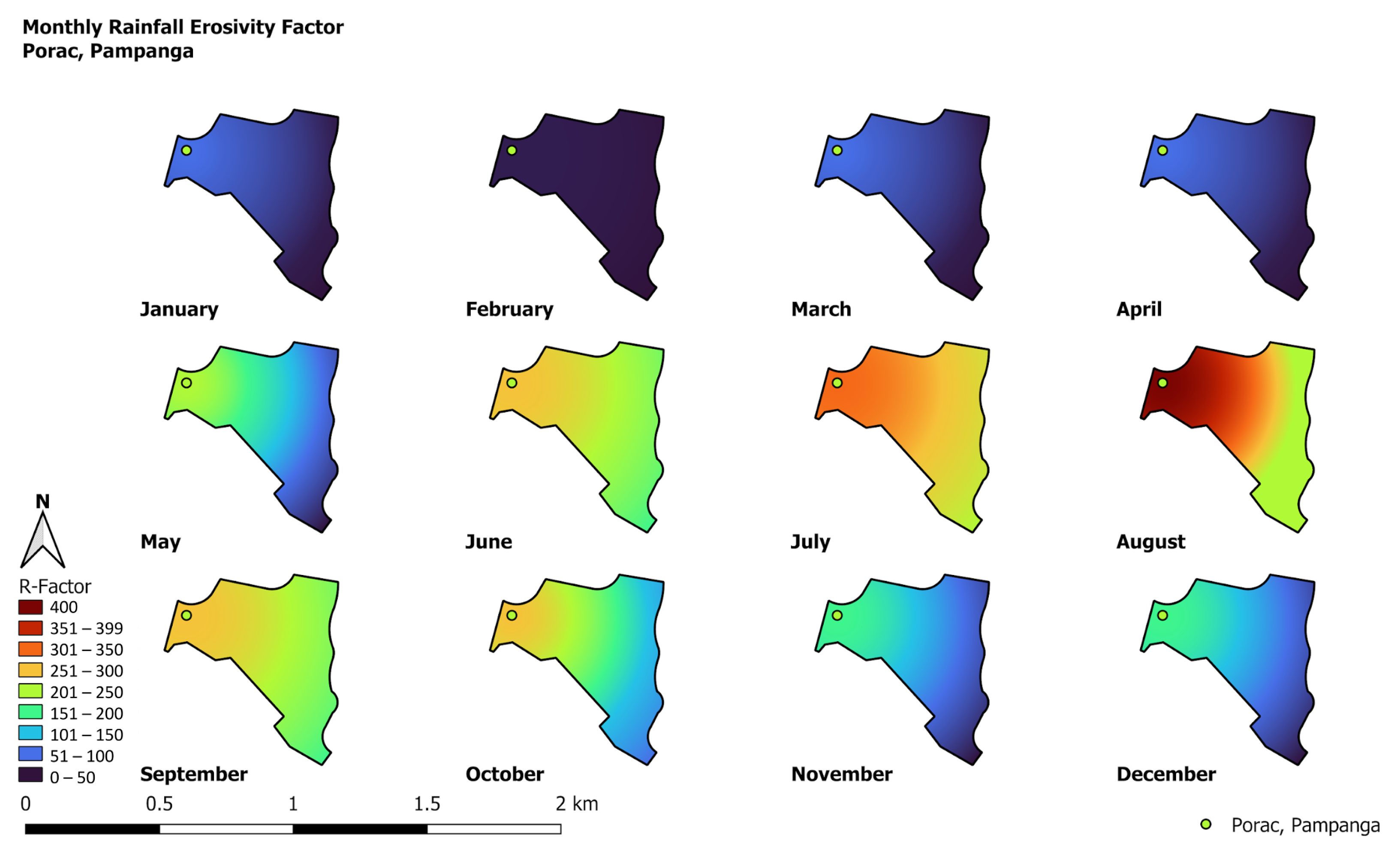
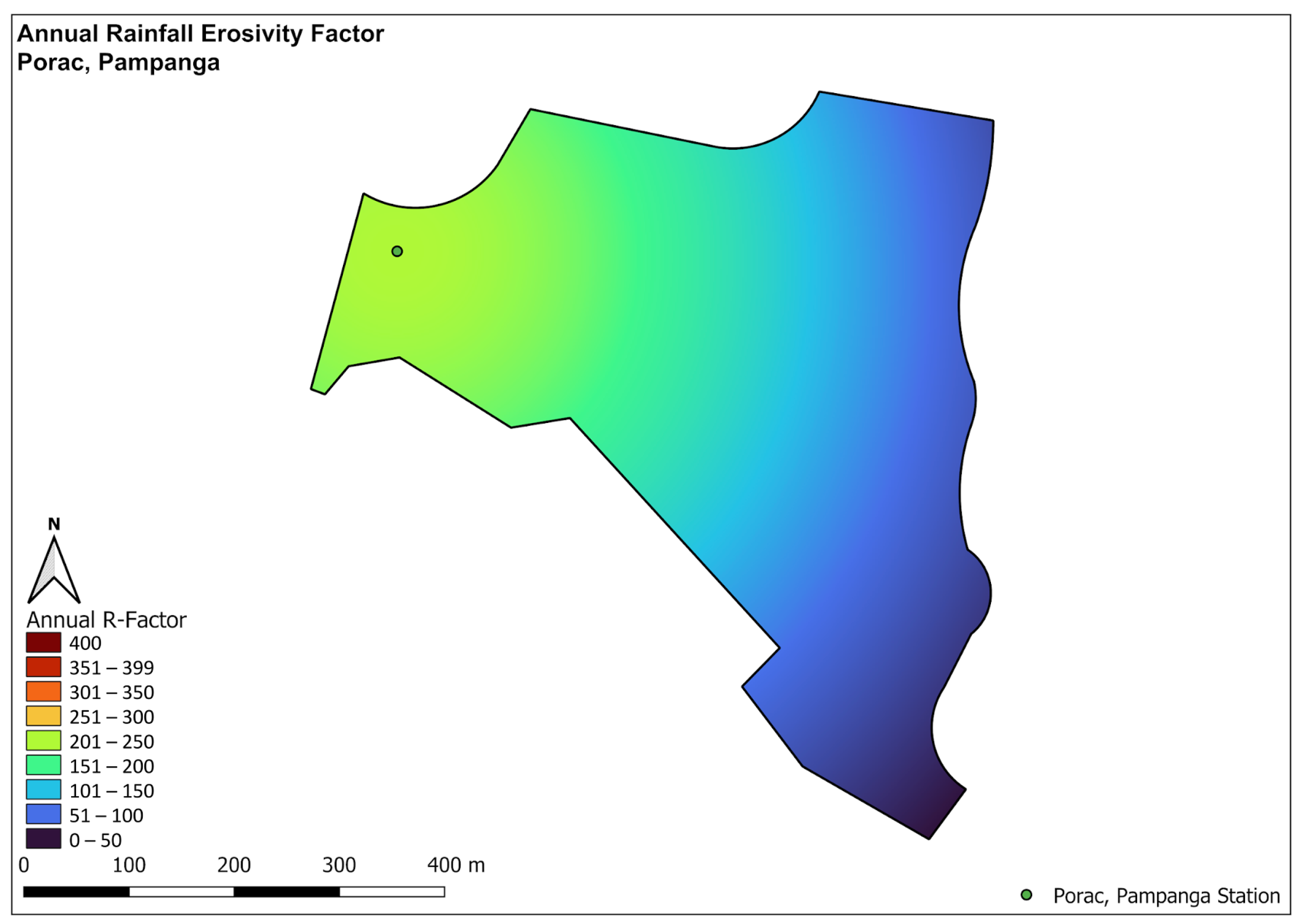
2.3. R-Factor Determination and Mapping

A strategy was established for deriving an empirical equation to determine the R-factor for the research location. During the development phase, the collected rainfall statistics were utilized as trial data for the study site.

As a result, several R-factor equations utilized in diverse global regions were compiled from previously published research. The relevance of these existing equations was subsequently evaluated according to the site classification obtained from the site analysis to ascertain their application under the conditions of the research site.

Adjustments were implemented to the R-factor equations across several climatic zones, considering alterations in precipitation characteristics, climatic patterns, and soil properties, which influence the erosive potential of rainfall in distinct geographical regions. Eight R-factor equations were chosen to apply in areas with comparable climatic circumstances to the research site, characterized by a tropical environment with two seasons.

Table 2. Summary of the R-factor formulas used in the development of the empirical R-factor equation on the study site.

Reference	Equation	Variables	Equation Number	Remarks
1957 [10]	$R={\displaystyle \frac{E\times I_{30}}{100}}$	E = total kinetic energy I30 = maximum 30 min rainfall intensity	(3)
2001 [13]	$R={\displaystyle \frac{1}{N}}{\displaystyle \sum _{i=1}^N}{\displaystyle \sum _{m=1}^{12}}{(7.05{rain}_{10}-88.92{\times days}_{10})}_{m,i}$	N = number of years of analysis rainn = monthly rainfall amount when rainfall ≥ 10 mm daysn = number of days when rainfall ≥ 10 mm m = month index i = year index	(4)
1996 [14]	$R=r\times a$	r = mean annual rainfall a = constant variable	(5)	Tested a = 0.5445
1992 [15]	$R=117.6\times \left({1.00105}^{AAP}\right)$	AAP = average annual precipitation	(6)	Tested a = 0.7824
1980 [16]	$R={\displaystyle \sum _{i=1}^{12}}1.735\times {10}^{(1.5\left({\displaystyle \frac{P_i}{P}}\right)-0.08188)}$	P = average annual rainfall amount Pi = average monthly rainfall amount	(7)	Tested a = 0.1345
1985 [17]	$R=-8.12+(0.562\times P)$	P = average annual rainfall amount	(8)
1986 [18]	$R=P\times 0.5$	P = average annual rainfall amount	(9)	Tested a = 0.1701
1981 [19]	$R=79+0.363AAP$	AAP = average annual precipitation	(10)	Tested a = 0.1868

summarizes the R-factor equations employed in formulating the empirical R-factor equation at the research location.

The equations compiled in Table 2 served as the primary foundation for the development. The similarities among these equations were evaluated using rainfall data, and the most accurate description of the research site was identified. The R-factor estimations derived from the evaluation were further analyzed using the generic R-factor equation.

Equation (3) delineates the often-employed general formula for determining the rainfall erosivity factor, as established by Wischmeier and Smith. This equation employs rainfall intensity and kinetic energy to assess the erosive potential of a particular rainfall event [11]. The intensity of rainfall may fluctuate considerably between various occurrences, and its effect on erosivity can be affected by factors like the duration and frequency of the rainfall event. Consequently, to get a more precise estimation of the erosivity of a rainfall event, it was essential to account for rainfall intensity at shorter intervals, namely every 30 min, which constituted one of the formula’s components. The erosivity index was computed by utilizing the total kinetic energy of precipitation and the 30 min rainfall intensity data to estimate the general R-factor. The equation of Wischmeier and Smith was used as the control variable.

Equation (4) was formulated based on the equation established by Loureiro and Coutinho [13], considering the duration of analysis in years, the monthly precipitation volume, and the number of days within a month that had rainfall of a certain depth. A precise assessment of the R-factor for a particular site necessitated the availability of mul-ti-year rainfall data. The formula accounted for the monthly precipitation alone when it was greater than or equal to 10 mm, the count of days within a month with precipitation above or equal to 10 mm, and the number of years included in the analysis.

Equation (5) was derived from the equation proposed by Roose [14], which calculates the primary rainfall erosivity factor over a decade using a constant variable given by the site’s topographic features and the mean annual rainfall. A general constant of 0.05 is utilized, whereas 0.1 is designated for the Mediterranean mountainous regions, 0.2 to 0.3 for tropical mountainous areas, and 0.6 for places within a 40 km proximity to the sea. This research examined all conceivable constant variables for the study area, especially assessing the range of 0.2 to 0.3 for tropical mountain regions with intervals of 0.01. Equation (6), created by Kassam et al. [15], solely considers the region’s average annual precipitation by utilizing the total annual rainfall and the yearly average to derive the annual R-factor for the location. Equation (7), proposed by Arnoldus et al. [16], integrates the average monthly and annual rainfall as variables to obtain the R-factor for the area. The equation evaluates the erosive potential of rainfall events by including both variables, facilitating a precise calculation of the R-factor.

In Equation (8), formulated by Hurni [17], the only variable examined was the average yearly rainfall. Likewise, Equation (9), formulated by Morgan [18], derived its estimation for the R-factor from the mean annual precipitation. The formula employed the product of the mean annual rainfall and a fixed value of 0.5 to calculate the R-factor for the region. Equation (10), proposed by Singh [19], utilized a notion akin to Hurni, wherein the average yearly precipitation was applied to compute the R-factor.

It was observed from the R-factor equations used in the study that constant factors were included to obtain the rainfall erosivity of an area. These constant factors were either stated in the equations developed or dependent on the climatic and topographic conditions of the region. With this observation, the researchers considered using constant variables with the rainfall amount data to establish a rainfall erosivity factor equation for the research site.

The annual rainfall erosivity factor (R) of the research site can be obtained by calculating the average rainfall erosivity for each month. The monthly rainfall erosivity factor and annual rainfall erosivity factor for the research site were then obtained with Equations (11) and (12), respectively, where R_i was the monthly rainfall erosivity factor measured in MJ/ha mm/h, P_i was the total monthly rainfall amount measured in mm, a was the constant to be tested, and R was the annual rainfall erosivity factor measured in MJ/ha mm/h.

$$R_i=P_i\times a$$

(11)

$$R={\displaystyle \frac{\sum R_i}{12}}$$

(12)

Once the constant variables (a) were obtained, as shown in Table 1, these were then multiplied with the total monthly precipitation amount (P_i) to obtain the monthly rainfall erosivity factor (R_i). In estimating the monthly rainfall erosivity factor, the average and maximum rainfall per month were also considered for the testing. The rainfall erosivity factor obtained from the average monthly rainfall and maximum rainfall per month was significantly lower and unrealistic compared to the estimated rainfall erosivity factor obtained from the general formula. Due to this, the results for testing average monthly rainfall and maximum rainfall per month were no longer included in the paper.

The Quantum Geographic Information System (QGIS) software version 3.28.3 ‘Firenze’ was employed to analyze the created R-Factor formula for the study site via temporal mapping. The temporal mapping was performed to evaluate the developed R-factor formula and its capacity to estimate rainfall erosivity at the study location.

3. Results

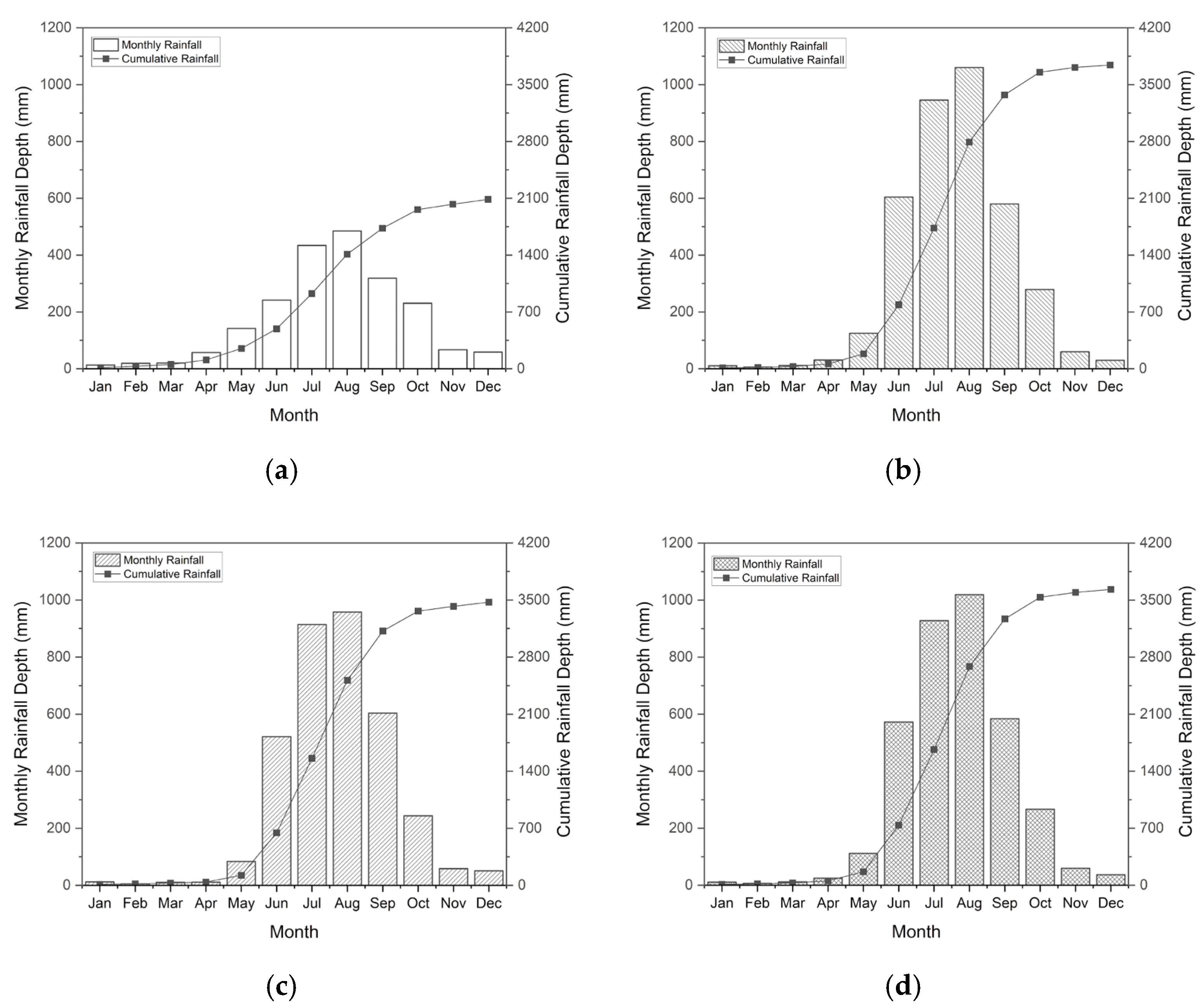
3.1. Rainfall Characteristics

The rainfall data obtained from the PAGASA stations and the IDW approach were evaluated to comprehend each location’s distinct features. Figure 2 compares the total rainfall quantities from four distinct stations: Clark, Iba, Cubi Point, and Porac.

From June to October, the peak rainfall months contributed around 90.18% of the total annual precipitation. Many tropical cyclones were documented at the specified stations, with around two to four occurring during the highest rainfall months [20]. This illustrated the disparity between the rainy and dry seasons across the four locations. The Clark station recorded a maximum rainfall of 484.7 mm in August and a low of 12.86 mm in January. Data from the Iba station indicate that August received the maximum rainfall, totaling 1060 mm, while February experienced the minimum with 6.25 mm. The Cubi Point station had a tendency analogous to that of the Iba station, with a maximum rainfall depth of 957.7 mm in August and the lowest rainfall depth of 5.45 mm in February. The Porac station recorded a maximum rainfall of 1019 mm in August and a low of 6.176 mm in February.

Figure 2 indicates that the Clark station had the lowest average rainfall. Data suggest that Iba station and Cubi Point station, two proximate places, saw far more significant rainfall than Clark. Despite being physically apart from Clark, these two stations had analogous rainfall accumulation patterns. The average predicted rainfall quantity calculated by the IDW approach for the Porac station was much greater than the actual rainfall recorded at the next station, Clark. The projected rainfall quantity closely corresponded with the actual precipitation seen at Iba and Cubi Point. The rainfall depths recorded at Iba and Cubi stations are considerably greater than those at Clark station, potentially affecting the estimated rainfall depth at Porac station. Nonetheless, the rainfall estimates at the Porac station are regarded as satisfactory, given that the climatic classification for all stations is Type I, according to a climate map produced by PAGASA [21].

The accuracy of the IDW method was validated by combining indirect assessments and comparisons with observed data. The rainfall estimates from IDW interpolation were cross-referenced with recorded precipitation values from the nearest available stations for consistency. The interpolated values were also checked for conformity with known patterns of rainfall in the area, such as seasonal changes and peak periods of rainfall. Although no test against alternative interpolation methods was carried out directly, the method’s capability to generate expected rainfall distributions and trends suggests suitability for the study.

Table 3. Mean ± SD ratios to estimate rainfall depth from the PAGASA (2012–2021) to the NASA (2012–2021) and GWC (2011–2020) data sets [22,23,24,25].

Month	Rainfall Depth (mm)			Ratio Relative to PAGASA
	PAGASA	NASA	GWC	NASA	GWC
January	11.01 ± 17.1	36.36 ± 27.0	24.29 ± 24.4	3.4 ± 1.2	2.3 ± 1.2
February	6.176 ± 5.21	37.06 ± 28.9	21.78 ± 19.2	6.1 ± 2.6	3.6 ± 2.6
March	11.43 ± 12.0	38.06 ± 32.3	34.40 ± 33.2	3.4 ± 1.3	3.1 ± 1.3
April	24.88 ± 13.8	53.86 ± 53.1	79.01 ± 51.5	2.2 ± 1.1	3.2 ± 1.1
May	111.8 ± 63.9	131.1 ± 57.4	132.2 ± 60.2	1.2 ± 0.1	1.2 ± 0.1
June	572.3 ± 307	384.3 ± 169	109.7 ± 95.9	0.7 ± 0.4	0.2 ± 0.4
July	928.0 ± 408	551.9 ± 191	154.4 ± 115	0.6 ± 0.4	0.2 ± 0.4
August	1019 ± 510	637.4 ± 327	131.1 ± 117	0.7 ± 0.4	0.2 ± 0.4
September	583.9 ± 300	441.7 ± 160	142.7 ± 145	0.8 ± 0.4	0.3 ± 0.4
October	266.8 ± 170	283.5 ± 175	113.9 ± 119	1.1 ± 0.3	0.5 ± 0.3
November	59.27 ± 61.9	125.2 ± 162	79.23 ± 77.2	2.2 ± 0.6	1.4 ± 0.6
December	36.76 ± 47.4	120.5 ± 100	77.32 ± 65.1	3.3 ± 1.2	2.2 ± 1.2
Annual	302.6 ± 75.7	236.7 ± 46.8	91.66 ± 53.4	2.1 ± 1.7	1.5 ± 1.3

presents rainfall depth mean and standard deviation for the datasets sourced from PAGASA, NASA-POWER, and GWC. The calculated ratio for each dataset was included in the table to facilitate the establishment of a link between the PAGASA dataset and the worldwide datasets from NASA-POWER and GWC. These ratios enabled the estimation of rainfall with a certain degree of accuracy, facilitating the comprehension of rainfall patterns at the station. Based on the table, the month of August recorded the most significant rainfall depth in the studied area. Conversely, January, February, and March often saw the lowest precipitation levels. The comparison of monthly rainfall levels from each dataset revealed substantial variations in the numbers across the datasets. The precipitation data collected from GWC were inferior to the rainfall measurements recorded by PAGASA and NASA-POWER. Among the three datasets, August demonstrated the greatest rainfall depths, apart from the GWC data, which recorded the maximum rainfall depth of 154.4 mm in July. Furthermore, analysis of the precipitation levels during the peak rainfall indicated that the rainfall quantities documented by NASA and GWC were underestimated compared to the local dataset from PAGASA. These inconsistencies may result in erroneous predictions due to the inadequate representation of peak rainfall occurrences in the data collection.

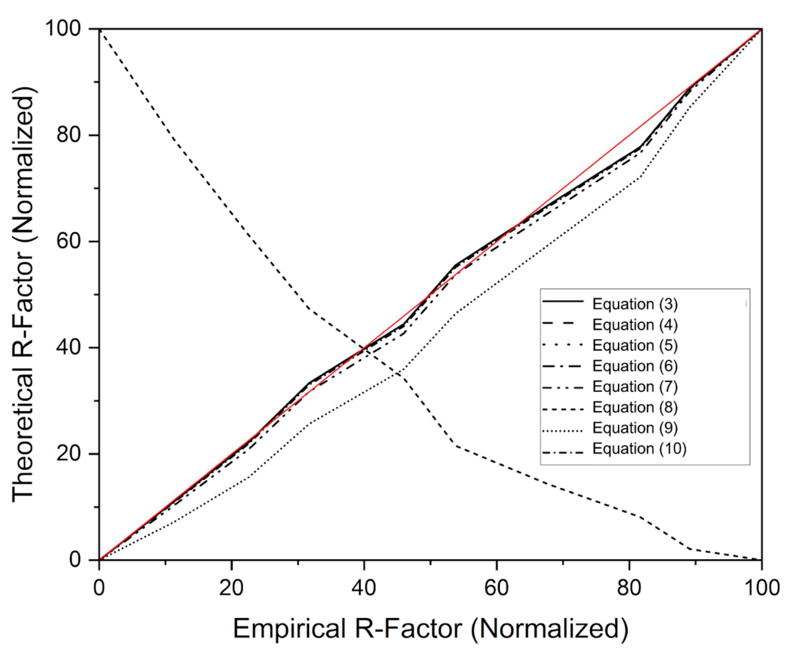
3.2. R-Factor Equations

The variation in R-factor equations was mainly caused by the climatic and geographical factors of the location where the equation originated. Rainfall patterns, storm strength, and topography can all vary drastically in different locations, resulting in variances in rainfall erosive potential. To acquire more precise estimates of the rainfall erosivity factor, several researchers developed customized equations modified to their specific local conditions. In applying rainfall erosivity factor equations for erosion assessments, it was essential to consider the equation’s origin. The erosive potential of rainfall in the particular area of interest may not be precisely reflected by an equation developed from a different region.

The gathered existing R-factor equations were assessed by applying the datasets from PAGASA, NASA-POWER, and GWC to estimate the R-factor of the research site, as presented in

Table 4. Annual R-factor estimates for each tested equation using the datasets of PAGASA, NASA, and GWC.

Reference	Eqn No.	R-Factor (MJ/ha mm/h)
		PAGASA	NASA	GWC
1957 [10]	(3)	88.75	-	-
2001 [13]	(4)	19,254	13,055	5161
1996 [14]	(5)	108.9	85.23	33.00
1992 [15]	(6)	118.4–119.3	118.4–118.9	117.7–118.4
1980 [16]	(7)	23.68–28.78	20.07–25.28	18.69–23.42
1985 [17]	(8)	−4.533–−0.433	−0.4707–−2.180	−7.446–−4.497
1986 [18]	(9)	3.191–6.839	3.037–5.285	0.599–3.223
1981 [19]	(10)	81.32–83.97	81.20–82.84	79.44–81.34

. The equation developed by Loureiro and Coutinho (Equation (4)) yielded significantly high and variable rainfall erosivity factors when applied to the datasets from PAGASA, NASA, and GWC. These values were deemed too high for the research site, possibly due to the conditions of the location where the equation was developed and applied. Loureiro and Coutinho developed and applied the formula as in ref. [13]. In Portugal, specifically in the Algarve region. Additionally, a study by Ranzi et al. [26] considered several data sets from 1959 to 2007, which amounts to 48 years of data. In contrast, only ten years of data were considered for the research site due to the lack of data.

From the analysis results from Equation (5) or the equation of Roose, the most conservative variable used in the research site was 0.3, resulting in estimates with almost similar values to the R-factor obtained from the general formula. A significant finding was that the different datasets produced varied estimates: PAGASA estimated 108.9 MJ/ha mm/h, NASA estimated 85.23 MJ/ha mm/h, and GWC estimated 33.00 MJ/ha mm/h. Similarly, the Kassam equation (Equation (6)) and the Arnoldus equation (Equation (7)) also provided relatively close values and the general formula.

However, the Hurni equation (Equation (8)) yielded negative values for all data sets, which indicated the inapplicability to the research site, potentially due to insufficient or too low rainfall amounts found within the research site. The formula was developed by Hurni in Ethiopia, and further studies on rainfall erosivity that used this formula were also conducted for the Koga watershed and Upper Blue Nile basin in Ethiopia [17]. Equation (9), the Morgan equation, produced rainfall erosivity factors that were relatively close to each other but significantly different from the value obtained from the general equation. The estimated R-factor from this equation produced the lowest applicable values for the research site, which spanned from 0.599 MJ/ha mm/h as the lowest estimate and 6.839 MJ/ha mm/h being the highest estimate. Finally, Equation (8), the Singh equation, yielded estimates that were the closest to the rainfall erosivity factor obtained from the general equation, which suggested its reliability for the research site.

These results indicated the variable effectiveness and applicability of the equations in estimating the R-factor for the research site. Some equations that produced high values, negative values, or large deviations from the general equation demonstrated the significance of meticulously selecting and evaluating equations based on their applicability to the specific study area.

It was observed from the table that the equation developed by Loureiro and Coutinho produced the highest values for the R-factor, considering that the other equations only provided R-factor values of up to 120. This suggested that this equation was better suited to environments or conditions with heavy precipitation or extremely erosive rainfall. Similarly, the equation developed by Hurni also stood out from the other equations since it consistently produced negative R-factor values. It was hypothesized that the formula could only produce accurate and precise data for locations with similar climatic or topographic conditions to Ethiopia.

In contrast, the developed R-factor equation took these as a basis and introduced a calibrated approach tailored to the tropical climate and limited data availability of the research site. Unlike the equations of Loureiro and Coutinho or Hurni, which showed extreme deviations, the developed equation closely aligns with observed rainfall erosivity values, thus offering greater applicability in tropical regions. Although comparable to the more straightforward models like Roose or Singh, the new equation uses locally scaled constants and IDW interpolation, making it much more adaptive and accurate. It ensures robustness even with minimal available datasets regarding rainfall, thus facilitating the consistent and reliable alternative to the soil erosion modeling in similar environments.

The equations of Roose, Kassam, Arnoldus, Morgan, and Singh were considered the most applicable formulas for the research site to obtain the constant variable to be used in the formula to be developed, due to their applicability to the research site. Each constant variable obtained from Table 1 was tested in the developed rainfall erosivity factor formula in Equation (11) using the datasets of PAGASA, NASA, and GWC. The monthly rainfall erosivity factors (R_i) and the annual rainfall erosivity factors (R) from Equation (1) were collected and compared. From the analysis of each constant variable for each equation, the variables that obtained a value closest to the estimated R-factor of the general formula are the constants from Singh and Roose.

4. Discussion

4.1. Developed Rainfall Erosivity Factor Equation

The rainfall erosivity factor from the general formula of 88.75 MJ/ha mm/h was inputted into the five applicable equations to obtain the site-specific constant variable. The rainfall amount data used were from the PAGASA, NASA, and GWC datasets applied in the testing, while the constant variables in the equation were kept unknown. The average of the constant variables from the three datasets was then collected and then divided by twelve for each of the equations to make the variable applicable for obtaining the monthly rainfall erosivity factor of the research site.

A study conducted by Adediji et al. [27] applied the Roose equation for their assessment conducted in Nigeria. From the evaluation, the rainfall amounts recorded in the area were significantly higher, with R-factor estimates that spanned from 270 MJ/ha mm/h to 450 MJ/ha mm/h with average annual rainfall amounts of 600 mm to 1000 mm. Singh’s formula was applied in a study conducted in India by Vinay and Mahalingam [28], which quantified soil erosion by water. It was found from the study that the R-factor, when utilizing the developed formula of Singh, presented estimates of 257.7 MJ/ha mm/h to 364.9 MJ/ha mm/h with recorded average annual rainfall from 500 mm to 700 mm. The values obtained in both studies validate the estimates gathered for the Porac station, as varying extreme rainfall events caused the difference in estimates. The significantly higher rainfall amounts observed in both Nigeria and India compared to the Porac station resulted in a more significant impact of rainfall on erosion in the areas.

From the comparisons conducted, it was found that the variable from Singh produced the most consistent R-factor and was considered the most conservative. From this comparison, the constant variable to be used in the formula follows the variable obtained from Singh’s equation. The developed rainfall erosivity factor equation for the research site is seen in Equation (13).

$$R_i=P_i\times 0.1868$$

(13)

From the analysis of each rainfall erosivity factor, Figure 3 presents a theoretical vs. empirical normalized plot that compares the results obtained from the eight tested existing R-factor equations with the equation developed for the study. The data presented in Figure 3 showed that the Equations (3)–(7) and (10) have similar normalized values compared to the generated equation. A certain degree of accuracy and dependability with these predictions can be assumed from the close match of the normalized values between these equations and the developed equation.

The finding confirms that the developed equation is compatible with the existing R-factor formulas. However, the derived equation and the other tested equations show some discrepancies with the Equations (8) and (9). The Equation (8) exhibits a distinctive trend, with a descending graph caused by pessimistic estimates due to the incompatibility of the equation to the study site. On the other hand, Equation (9) displays an upward trend similar to the previous equations. However, in terms of the normalized values, it deviates significantly further from the produced equation. This deviation was caused by the constant variable, 0.5, used in the equation, which was calibrated to the rainfall conditions specific to the rainfall in India [18].

4.2. GIS Rainfall Erosivity Analysis

Figure 4 shows the rainfall erosivity factor mapping for each month of the research area. Notably, August stands out among the other months studied with the highest R-factor of 371.3 MJ/ha mm/h, which indicates that it experienced the most erosive rainfall conditions. This observation confirms that August in the study area was characterized by strong precipitation episodes that had significant impacts on soil erosion. The lowest R-factor, on the other hand, was exhibited in February with an R-factor range of 0.096 MJ/ha mm/h to 2.901 MJ/ha mm/h, which suggests that rainfall erosivity is comparatively low during this month. The lower erosivity factor in February indicated less intense rainfall or a reduced risk of soil erosion. These months presented nearly identical values by comparing the R-factors of January, March, and April. These estimates are also notably low, with values similar to those in February. Similarly, the R-factor values for June and September were almost identical, indicating comparable rainfall erosivity levels throughout these months.

Figure 5 presents an annual R-factor map of the research site, providing a complete perspective of the whole range of R-factor estimates throughout the study period. The erosive potential of the research area over the year was further understood from this diagram. Through the annual R-factor data from the different points with the analysis from Figure 5, the R-factor range varied from 1.153 MJ/ha mm/h to 190.3 MJ/ha mm/h, which accurately represented the erosivity of rainfall around the area. Throughout the year, it was noted that the erosivity of rainfall within the research site varied greatly depending on the season and conditions.

The study of Vinay and Mahalingam [28] presented the R-factor estimates of their research conducted in India. It gave a similar pattern to Figure 5, which showed a varied range of R-factor estimates throughout the year. Similarly, compared to the study of Joshi et al. [29], who assessed soil loss in a watershed in India, a comparable trend was found. Like the Porac station, India is considered a tropical wet and dry climate type. Locations with this type of climate tend to experience varied rainfall amounts throughout the year due to changing patterns in monsoons, trade winds, and other climatic factors. The figures shown in both studies, as well as for the Porac station, presented a wide range of estimates for the annual R-factor, further confirming the developed formula’s acceptability and reliability.

Overall, this study advances soil erosion modeling in data-scarce tropical regions by addressing some challenges and limitations in existing methodologies. The developed empirical equation proved to be reliable in estimating the R-factor across the study area. The results not only enhance the accuracy of soil erosion predictions but also provide a practical framework for addressing data gaps in similar contexts. Unlike the many existing equations that are data-intensive or require sophisticated facilities, the proposed method utilized the IDW interpolation technique and localized calibration to provide adequate rainfall data in data-scarce contexts. It supports more effective soil conservation and watershed management strategies through the application of results in different soil loss models by lining up with available models and providing a region-specific approach; this is especially the case in tropical developing regions where erosion is a significant challenge in implementation and execution,. This work bridges methodological gaps to support more accessible and reliable soil conservation practices, especially for resource-constrained regions.

5. Conclusions

The research on rainfall erosivity emphasized the significance of obtaining the R-factor to effectively manage and assess soil erosion and implement appropriate erosion control techniques. In particular, the significant findings of the study include the following:

(1)

Rainfall depth estimates obtained from global resource platforms did not properly represent the peak rainfall events within the year.

(2)

The accuracy of the estimates obtained from different R-factor equations varied depending on the specific climatic and topographic conditions of the location where the equation originated.

(3)

Multiple R-factor equations tend to use similar parameters, such as variations of rainfall data with other variables and constants, to estimate the erosivity of rainfall in a specific area.

It was concluded that this research helped in the interpretation and understanding of soil loss modeling techniques by developing an empirical equation to calculate rainfall erosivity. However, there were certain limitations identified that validate a need for further research. The assumption of spatial uniformity by using IDW interpolation may not have considered the climatic variations impacted through factors such as topography or land use. Furthermore, since the equation is mainly based on the monthly and annual patterns of rainfall and mostly controlled by extreme rainstorms, the high resolution for short-termed erosive events becomes lower.

Future studies may look at integrating other geostatistical techniques such as Kriging, Spline, or other machine learning models into precipitation interpolation accuracy. Future study can also be expanded to cover more extended durations or add other stations in the area which may make the developed equations more adaptable. Furthermore, the nonlinear interactions among rainfall, soil properties, and land cover highlighted the need for interdisciplinary approaches that combine hydrology, soil science, and remote sensing to refine soil erosion predictions. Improving these challenges would bring the applicability of the findings into more effective conservation strategies in diverse environments.

The study also underlined the importance of accurate and up-to-date rainfall data, which were essential for the accuracy and consistency of the developed equation. Based on the study, it was found that in addition to its ability to estimate the R-factor, the research could aid with estimating rainfall data in data-scarce areas through indirect approaches of determining rainfall amounts in locations where rainfall data may be limited or unavailable. The developed methodology could be utilized in data-scarce regions, similar to the research site, to obtain the R-factor, enabling its application in different soil loss models for various watersheds.

References

1. Admas, B.F.; Gashaw, T.; Adem, A.A.; Worqlul, A.W.; Dile, Y.T.; Molla, E. Identification of soil erosion hot-spot areas for prioritization of conservation measures using the SWAT model in Ribb watershed, Ethiopia. Resour. Environ. Sustain. 2022, 8, 100059. [Google Scholar] [CrossRef]
2. García-Ruiz, J.M.; Beguería, S.; Lana-Renault, N.; Nadal-Romero, E.; Cerdà, A. Ongoing and emerging questions in water erosion studies. Land Degrad. Amp. Dev. 2016, 28, 5–21. [Google Scholar] [CrossRef]
3. Benchettouh, A.; Kouri, L.; Jebari, S. Spatial estimation of soil erosion risk using RUSLE/GIS techniques and practices conservation suggested for reducing soil erosion in Wadi Mina watershed (northwest, Algeria). Arab. J. Geosci. 2017, 10, 79. [Google Scholar] [CrossRef]
4. Meng, X.; Zhu, Y.; Yin, M.; Liu, D. The impact of land use and rainfall patterns on the soil loss of the hillslope. Sci. Rep. 2021, 11, 16341. [Google Scholar] [CrossRef] [PubMed]
5. Igwe, P.U.; Onuigbo, A.A.; Chinedu, O.C.; Ezeaku, I.I.; Muoneke, M.M. Soil Erosion: A Review of Models and Applications. Int. J. Adv. Eng. Res. Sci. 2017, 4, 138–150. [Google Scholar] [CrossRef]
6. Borrelli, P.; Alewell, C.; Alvarez, P.J.M.; Anache, J.A.A.; Baartman, J.; Ballabio, C.; Bezak, N.; Biddoccu, M.; Cerdà, A.; Chalise, D.; et al. Soil erosion modelling: A global review and statistical analysis. Sci. Total Environ. 2021, 780, 146494. [Google Scholar] [CrossRef] [PubMed]
7. Kinnell, P. Event soil loss, runoff and the Universal Soil Loss Equation family of models: A review. J. Hydrol. 2010, 385, 384–397. [Google Scholar] [CrossRef]
8. Delgado, M.E.M.; Canters, F. Modeling the impacts of agroforestry systems on the spatial patterns of soil erosion risk in three catchments of Claveria, the Philippines. Agrofor. Syst. 2011, 85, 411–423. [Google Scholar] [CrossRef]
9. Schmitt, L.K. Developing and applying a soil erosion model in a data-poor context to an island in the rural Philippines. Environ. Dev. Sustain. 2007, 11, 19–42. [Google Scholar] [CrossRef]
10. Wischmeier, W.H.; Smith, D.D. Predicting Rainfall Erosion Losses: A Guide to Conservation Planning; Handbook; Science and Education Administration, US Department of Agriculture: Washington, DC, USA, 1978; p. 537.
11. Wischmeier, W.H.; Smith, D.D. Factors affecting sheet and rill erosion. Transactions 1957, 38, 889. [Google Scholar] [CrossRef]
12. Khouni, I.; Louhichi, G.; Ghrabi, A. Use of GIS based Inverse Distance Weighted interpolation to assess sur-face water quality: Case of Wadi El Bey, Tunisia. Environ. Technol. Innov. 2021, 24, 101892. [Google Scholar] [CrossRef]
13. Loureiro, N.; Coutinho, M.S.S. A new procedure to estimate the RUSLE EI30 index, based on monthly rainfall data and applied to the Algarve region, Portugal. J. Hydrol. 2001, 250, 12–18. [Google Scholar] [CrossRef]
14. Roose, E.; Lal, R. Introduction to the Conservation Management of Water, Biomass and Soil Fertility (GCES) [FAO Corporate Document Repository]. 1994. Available online: https://horizon.documentation.ird.fr/exl-doc/pleins_textes/divers15-05/010012051.pdf (accessed on 15 June 2023).
15. Kassam, A.; Velthuizen, H.; Mitchell, A.; Fischer, G.; Shah, M. A Case Study of Kenya Resources Data Base and Land Productivity Technical Annex 2 Soil Erosion and Productivity. Agro-Ecological Land Resources Assessment for Agricultural Development Planning; Food and Agriculture Organization (FAO): Rome, Italy, 1991. [Google Scholar]
16. Arnoldus, H.M.J. An Approximation of the Rainfall Factor in the Universal Soil Loss Equation. An Approximation of the Rainfall Factor in the Universal Soil Loss Equation; John Wiley and Sons: Hoboken, NJ, USA, 1980; pp. 127–132. [Google Scholar]
17. Hurni, H. Soil Conservation Manual for Ethiopia: A Field Guide for Conservation Implementation; Community Forests and Soil Conservation Development Department: Addis Abeba, Ethiopia, 1985. [Google Scholar]
18. Morgan, R.P.C. Soil Erosion and Conservation; John Wiley Sons: Hoboken, NJ, USA, 2009. [Google Scholar]
19. Singh, G. Soil Loss Prediction Research in India; Central Soil & Water Conservation Research & Training Institute: Kota, India, 1981. [Google Scholar]
20. Macalalad, R.V.; Badilla, R.A.; Cabrera, O.C.; Bagtasa, G. Hydrological response of the Pampanga River basin in the Philippines to intense tropical cyclone rainfall. J. Hydrometeorol. 2021, 22, 781–794. [Google Scholar] [CrossRef]
21. PAGASA. Climate of the Philippines. Department of Science and Technology Philippines. Available online: https://www.pagasa.dost.gov.ph/information/climate-philippines (accessed on 25 April 2023).
22. PAGASA. Climate and Agrometeorological Data Section. Rainfall Amount Data Set for Clark Airport, Pampanga Station [Data Set]; Philippine Atmospheric, Geophysical and Astronomical Services Administration: Quezon City, Philippines, 2021.
23. PAGASA. Hydrometeorological Data Application Section. Rainfall Intensity-Duration-Frequency for Zambales and Olon-Gapo Stations [Data Set]; Philippine Atmospheric, Geophysical and Astronomical Services Administration: Quezon City, Philippines, 2021.
24. National Aeronautics and Space Administration. Point Daily Humidity/Precipitation Data [Data Set]; NASA: Washington, DC, USA, 2021.
25. National Centers for Environmental Information. Daily Rainfall Data for Porac, Pampanga [Data Set]; American National Oceanic and Atmospheric Administration: Washington, DC, USA, 2020.
26. Ranzi, R.; Le, T.H.; Rulli, M.C. A RUSLE approach to model suspended sediment load in the Lo river (Vietnam): Effects of reservoirs and land use changes. J. Hydrol. 2012, 422–423, 17–29. [Google Scholar] [CrossRef]
27. Adediji, A. Assessment of Revised Universal Soil Loss Equation (RUSLE) in Katsina Area, Katsina State of Nigeria using Remote Sensing (RS) and Geographic Information System (GIS). Iran. J. Energy Environ. 2010, 1, 255–264. [Google Scholar]
28. Vinay, M.; Mahalingam, B. Quantification of soil erosion by water using GIS and remote sensing techniques. J. Earth Sci. 2015, 4, 103–110. [Google Scholar]
29. Joshi, V.; Susware, N.; Sinha, D. Estimating soil loss from a watershed in Western Deccan, India, using Revised Universal Soil Loss Equation. Acta Geogr. Debrecin 2016, 10, 13–25. [Google Scholar] [CrossRef]
Figure 1. Study area.
Water 17 00837 g001
Figure 2. Total monthly rainfall depth (mm) for (a) Clark station, (b) Iba station, (c) and Cubi Pt. station from PAGASA, and (d) Porac station from IDW method.
Water 17 00837 g002
Figure 3. Comparison of developed R-factor equation with existing R-factor equations [10,13,14,15,16,17,18,19].
Water 17 00837 g003
Figure 4. Monthly average R-factor estimate mapping using GIS.
Water 17 00837 g004
Figure 5. Annual average R-factor estimate mapping using GIS.
Water 17 00837 g005