Abstract
Accurate soil moisture (SM) estimates with high spatial resolution are highly desirable for agricultural, hydrological, and environmental applications. This study developed a two-step reconstruction approach to obtain a high-quality and high-spatial-resolution (0.05°) SM dataset from microwave and model-based SM products, combining Bayesian three-cornered hat (BTCH) merging and machine/deep learning downscaling algorithms. Firstly, a three-cornered hat (TCH) method was used to analyze the uncertainty of seven SM products on four main land cover types in the Pearl River Basin (PRB). On this basis, the SM products with low uncertainty were merged using the BTCH method. Secondly, two machine/deep learning algorithms (random forest, RF, and long short-term memory, LSTM) were applied to downscale the merged SM data from 0.25° to 0.05° based on the relationship between SM and auxiliary variables. The overall performance of RF and LSTM downscaling models with/without antecedent precipitation were compared. The merged and downscaled SM results were validated against in situ observations and the China Meteorological Administration (CMA) Land Data Assimilation System (CLDAS) SM data. The results indicated the following: (1) The BTCH-based SM estimate outperformed the parent products and the AVE-based SM estimate (the arithmetic average), indicating that BTCH is a fusion approach that can effectively reduce data uncertainties and optimize weights. (2) The optimal time scale for the cumulative effect of precipitation on SM was 35 days during 2015–2020 in the PRB. SM estimations using RF and LSTM downscaling algorithms both had substantial improvement by considering the antecedent precipitation variable, both at the 0.25° and 0.05° spatial scales. Feature importance assessment also revealed the most important role of antecedent precipitation (30.01%). Moreover, the LSTM model with antecedent precipitation performed slightly better than the RF model with antecedent precipitation. (3) The downscaled SM results all mitigated the overestimation inherent in the original SM data, though they were inevitably limited by the performance of the original SM data and difficult to surpass. The developed two-step reconstruction approach was effective in generating an accurate SM dataset at a finer spatial scale for wide regional applications.
1. Introduction
Soil moisture (SM) is a key state variable in the Earth’s system that controls the exchange of water and energy fluxes between the land surface and atmosphere [1,2], and it has been widely utilized in numerous disciplines and applications. Accurate and detailed SM information is highly desirable for many regional applications, such as droughts and floods [3,4], agricultural irrigation [5], and water resources management [6]. However, due to the common impact of meteorological, topographic, vegetative, and pedological factors [7,8], SM generally presents large spatiotemporal variability, and it is still challenging to obtain accurate SM data with high spatial resolution.
SM can be obtained through ground-based observations, remotely sensed estimation, and land surface modeling, each with their own strengths and limitations. Specifically, ground observations can provide precise SM estimation at multi-layer depths but are costly and labor-intensive, and they suffer a lot from the poor spatial representativeness of discrete information at particular points [9]. Satellite-based SM products can estimate spatially continuous SM of the surface soil layer (0–5 cm) at a large scale, but they contain considerable uncertainties caused by underlying conditions, instrumental deficiencies, and retrieval algorithms [10]. Land surface models can generate spatial completeness and temporal continuity SM simulations of different soil layers globally; however, their accuracy has unignorable errors from the model parameterization, model structure, and quality of forcing data [11]. Data merging is currently an effective solution to improve SM quality, which could overcome the drawbacks and combine the superiorities of each individual dataset [12]. Moreover, microwave and model-based SM products usually have relatively coarse spatial resolution (around tens of kilometers), greatly hindering their applications in many regional hydrological and agricultural studies. Hence, it was of great significance to acquire accurate SM data merging from multi-source datasets at a fine spatial resolution, particularly at the basin scale.
Data fusion can integrate multi-source datasets and knowledge into a better data product [13]. Linear weight averaging is the most common and preferable way for data fusion due to its simplicity, interpretability, applicability to any number of datasets, and visible improvements in practice [14]. The key to linear weight averaging is to calculate the weight values derived from the correlations or errors of the individual components to be fused. At present, triple collocation (TC) [15] and three-cornered hat (TCH) [16] are two commonly used methods for estimating the error variance of soil moisture retrievals without any a priori knowledge. The difference was that the TC method can only quantify the error variance of three mutually independent datasets, while the TCH method can be applied to more than three time series and considered the cross correlation among datasets [9]. Linear weighted data fusion based on TCH-derived error has been adopted in numerous data fusion studies focusing on various geophysical variables such as precipitation [17], gross primary productivity [18], and evapotranspiration [19]. Nevertheless, for SM, most research has been conducted on uncertainty analysis [20], with few focusing on the multi-source data fusion based on TCH uncertainty. Combining the satellite-based retrievals and model simulations can significantly reduce the uncertainties of SM data on a global scale [21]. Therefore, a TCH-based linear fusion of SM estimates from active and passive satellites and models is necessary to be investigated.
To obtain SM estimates with high spatial resolution, various spatial downscaling techniques have been proposed by accounting for the impact of numerous auxiliary variables, such as the regression fitting [22], the Disaggregation based on Physical And Theoretical scale CHange (DISPATCH) [23], the triangular/trapezoidal feature space [24], and machine/deep learning approaches [8]. The idea behind these methods is to establish either a statistical correlation or a physically based model between coarse-scale SM and fine-scale auxiliary variables [25]. There are two main differences among these methods, including different characteristics of downscaling models and different types of auxiliary input data. For downscaling model construction, machine/deep learning algorithms, such as random forest (RF) [2,26], long short-term memory networks (LSTM) [10], and convolutional neural networks (CNNs) [27], have received the most attention in recent years owing to their advantages in dealing with massive remote-sensed data and non-linear problems [28]. For auxiliary variables closely related to SM, land surface temperature (LST), vegetation index, surface albedo, brightness temperature, contemporary precipitation, SM memory, topographic factors, and soil texture are all widely applied in various SM downscaling models [2,8,26,29,30,31]. Based on the principle of water balance, the current soil water content is primarily determined by the effective precipitation that has occurred in the preceding period if no irrigation [32,33]. However, few studies have viewed antecedent precipitation as an important spatial downscaling feature. Thus, adding an antecedent precipitation variable to the downscaling model and considering the nonlinear relationship between SM and corresponding auxiliary variables may theoretically improve the estimation accuracy of SM.
Within this context, this study aimed to develop a two-step reconstruction approach based on the TCH-based linear fusion and machine/deep learning downscaling algorithms, which was designed to generate a high-quality pentad (5-day) SM dataset with a spatial resolution of 0.05° from microwave and model-based SM products. Specifically, the objectives of this study were (1) to identify the effectiveness of the TCH-based fusion method in improving SM data accuracy, (2) to evaluate the impacts of antecedent precipitation on downscaled SM quality in the spatial downscaling schemes, and (3) to validate the performance of the merged and downscaled SM results against in situ observations and the China Meteorological Administration (CMA) Land Data Assimilation System (CLDAS) SM data. The results of this study would be valuable in providing more detailed and accurate information on SM for regional hydrometeorological applications.
2. Study Area and Data
2.1. Study Area
The Pearl River Basin (PRB) is located in southern China (Figure 1), with a mainstem length of 2214 km and an area of 453,700 km2. This study area can generally be divided into three geographical zones from west to east, including the Yunnan–Guizhou Plateau, the Guangdong–Guangxi Hills, and the Pearl River Delta (PRD) [34], with elevations ranging from −55 to ~2933 m. Located in the subtropical monsoon climate zone, the PRB has an average annual temperature of 14 to 22 °C and average precipitation of 1200 to 2200 mm, with 80% of the total annual precipitation falling between April and September each year [26]. Influenced by the complex topography and climate, extreme hydrological events such as floods and droughts occur frequently in the basin, requiring detailed and accurate SM information. The PRD was not considered in this paper because the high imperviousness makes it difficult for the soil to store water through precipitation infiltration.
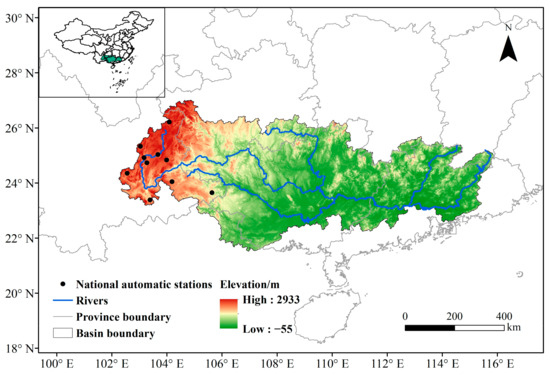
Figure 1.
Location, elevation, and soil moisture stations of the PRB.
2.2. Data
2.2.1. Soil Moisture Data
SM products used in this study included four microwave products (one active and three passive), three model-based products, and two validation datasets, with their main characteristics shown in Table 1.

Table 1.
Overview of SM data used in this study.
The active microwave product was derived from the European Space Agency’s (ESA) Soil Moisture Climate Change Initiative (CCI) project [35], hereafter referred to as CCI-active (version 7.1). The relative SM (%) was converted into volumetric unit (m3/m3) using soil porosity information from the ESA CCI.
Three passive microwave products included SM datasets from the Advanced Microwave Scanning Radiometer 2 (AMSR2) [36], the Fengyun-3C (FY-3C) [37], and the Soil Moisture Active Passive (SMAP) [38]. To reduce radio frequency interference influence [39], the Land Parameter Retrieval Model (LPRM) AMSR2 L3 X-band SM product was used (hereafter AMSR2). FY-3C is China’s second-generation polar-orbiting meteorological satellite that was launched in September 2013. For this study, the FY-3C L2 SM observations from April 2015 to February 2020 were used. The SMAP product used in this study was the level-3 daily SM product (version 8) posted on a 36 km grid using EASE-Grid 2.0. Daily SM for each of the three products was obtained by averaging their ascending and descending datasets.
Three model-based products included SM datasets from the land component of the 5th generation of European ReAnalysis (ERA5), referred to as ERA5-Land [40], NASA’s Global Land Data Assimilation System (GLDAS) [41], and the Global Land Evaporation Amsterdam Model (GLEAM) [42]. ERA5-Land hourly data provide SM estimates at four soil layers (0–7, 7–28, 28–100, and 100–289 cm), in which the top layer SM data were used. The GLDAS product used in this study was the GLDAS-2.1 Noah L4 3-hourly 0.25° data (hereafter GLDAS), which describes SM in four layers (0–10, 10–40, 40–100, and 100–200 cm), and the top 0–10 cm SM data were used. For GLEAM, the daily surface SM (0–10 cm) of version 3.6a was collected. The ERA5-Land hourly and GLDAS 3-hourly SM estimates were averaged to yield the daily SM.
In situ SM measurements and the CLDAS SM data (version 2.0) [43] were used as validation datasets. The CLDAS provides hourly SM in five layers (0–5, 0–10, 10–40, 40–100, and 100–200 cm), in which the top 0–5 cm SM data from January 2017 to December 2019 were applied. In situ observations were collected from China’s national meteorological stations, providing hourly SM from 10 to 100 cm depth with an interval of 10 cm, and the top 0–10 cm SM data were used. Hourly SM estimates from the CLDAS and in situ observation were averaged to obtain the daily value.
2.2.2. Auxiliary Data
Land cover type data were from GlobeLand30 [44] in the year 2020, with an overall classification accuracy of 85.72%. There are a total of six land cover types in the PRB, with cropland, woodland, grassland, and shrubland being the four main land cover types after water bodies and artificial surfaces are removed. Precipitation data were collected from the Climate Hazards Group Infrared Precipitation with Stations (CHIRPS) daily product. All-weather LST data were from the Global daily 0.05° spatiotemporal continuous land surface temperature dataset (2002–2022) hosted at the National Tibetan Plateau Data Center [45]. The datasets from four overpass times were averaged to obtain the daily LST. Enhanced Vegetation Index (EVI) data were collected from the MOD13C1 (v6.1). Quality control, linear interpolation, and Savitzky–Golay (S–G) filter [46] methods were applied to obtain a high-quality daily EVI dataset. Albedo data were obtained from the MCD43C3 (v6.1), in which shortwave black-sky albedo and white-sky albedo layers were quality controlled and used to calculate the real surface albedo [47]. Then, linear interpolation and S–G filter methods were also applied to generate a gap-filled and high-quality real surface albedo dataset. Digital elevation model (DEM) data were obtained from the NASA Shuttle Radar Topography Mission [48]. Elevation, slope, and aspect were extracted as topographical factors. Soil texture data (proportion of sand, silt, and clay content) were obtained from the Harmonized World Soil Database version 1.2 [49]. Table 2 lists the basic information of the above datasets.
Table 2.
Overview of auxiliary data used in this study.
2.2.3. Data Preprocessing
To ensure that all datasets had a uniform specification, data preprocessing was performed as follows. The time range of all SM and auxiliary datasets was unified from April 2015 to December 2020, except for the FY-3C and CLDAS. The spatial resolution of FY-3C, SMAP, ERA5-Land, and GlobeLand30 datasets was resampled to 0.25°, consistent with other SM products. The spatial resolution of DEM and soil texture data was resampled to 0.05°, consistent with other auxiliary products. The temporal resolution was unified as pentad (5-day average, and sum for precipitation), and the geospatial reference was set to GCS_WGS_1984.
3. Methods
3.1. SM Reconstruction Approach
Figure 2 shows the two-step SM reconstruction approach (first merging then downscaling) developed in this study. Note that the spatial downscaling was conducted based on an assumption that models established by auxiliary variables over an appropriate range of scales are applicable to SM reproduction [50]. The specific steps are described as follows:
- The TCH method was firstly used to analyze uncertainties of multiple SM products on different land cover types at a spatial resolution of 0.25°. The products with low uncertainties were then combined to produce a merged SM product using the BTCH merging method.
- All auxiliary variables including real albedo, precipitation, EVI, LST, soil texture (sand, clay, and silt), and terrain (elevation, slope, and aspect) were resampled to 0.25° spatial resolution, the same as the merged SM product.
- RF and LSTM models were constructed between the merged SM and auxiliary variables at a coarse spatial resolution (0.25°), and the corresponding downscaled SM was generated by inputting auxiliary variables at a high spatial resolution (0.05°). To explore if antecedent precipitation can improve the downscaling results, we trained the RF and LSTM models under two conditions each: with and without the antecedent precipitation, for comparison.
- The performances of each downscaled SM and the original (merged) SM product were evaluated using in situ observation and the CLDAS SM data, and they were inter-compared.
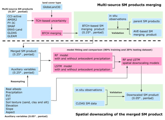
Figure 2.
The SM reconstruction approach developed in this study.
3.2. Bayesian Three-Cornered Hat (BTCH) Merging
Suppose there are N sets of SM products , corresponds to different products. According to the Bayesian theory, the probability density function (PDF) for the th SM product () can be expressed as
where is the true value of SM (actually, is not available and is a hypothetical true value, also representing the SM value after merging), and and are the zero-mean white noise and error variance of , respectively. L(•) is the likelihood function.
In the same way, the PDF for th SM product () can be expressed as
where and are the zero-mean white noise and error variance of , respectively.
The maximum likelihood of true SM () is the maximum value of its joint probability distribution:
To obtain the maximum likelihood value of , the cost function is defined as
Letting the first variation of be zero, , then could be obtained as
If we define , then
where and are weight values of and , respectively.
Similarly, for N sets of SM products, Equation (7) can be expressed as
The weight values of each SM product (e.g.,) are defined as
The error covariance () of each SM product is derived by the TCH method [16]. Since is not available, the difference series between (N − 1) SM products and a reference SM product () (chosen arbitrarily from N SM products) can be expressed as
Note that the error covariance results of the TCH method are independent of the selected reference dataset [51]. Store the (N − 1) difference sequence in the following matrix:
where is the difference matrix with M rows and (N − 1) columns (M is the number of each SM product). The covariance matrix of is given as
where is the covariance operator. The unknown covariance matrix of the individual noises ( is a symmetric matrix) is related to by
where is the identity matrix and can be defined as
and matrix is defined as
where . The question now is that unknowns cannot be solved for only equations. There remain N “free” parameters that must be reasonably determined to obtain a unique solution. To determine the N free parameters, an objective function is minimized based on the Kuhn–Tucker theorem [52], and it always fulfills the positive definiteness of . The objective function F is given by
with a constraint function H
where , is a diagonal matrix with elements on its diagonal, which can be obtained by minimizing Equation (17) through initial condition iterations [19]. are the error covariances that equal to , and their square roots represent the relative uncertainty of each SM product.
3.3. Machine/Deep Learning Algorithms
The details and parameters of RF and LSTM algorithms are as follows. Note that we randomly sampled 80% of the data to train the model, and the remaining data (20%) were used as a test dataset to verify the model performance [53]. A total of 80% of the data were mainly used to determine model parameters, i.e., grid search and cross-validation in the RF model and empirical parameters in the LSTM model. If the model performs comparably on both the training and test datasets, it indicates that this model is suitable for our dataset.
RF is a popular machine learning algorithm widely used in regression, in which a number of decision trees are first constructed during training phase, and then the mean prediction from these trees is generated as the prediction of the whole model [54]. To accurately estimate SM, a grid-search approach and 10-fold cross-validation were employed to automatically optimize and determine the key hyperparameters. The key hyperparameter values were as follows: the number of trees in the forest was 1000, the maximum features was 2, the minimum sample leaf was 1, the minimum samples split was 2, the mean squared error was used to measure the quality of a split, and bootstrap samples were used when building the trees.
LSTM is a special kind of recurrent neural network, and it can handle both long-term dependency problems and reduce the possibility of exponential explosion [55]. In this study, a two-layer LSTM structure was used, with a cell/hidden state length of 80 and 100. The output from the last LSTM layer at the last step was connected to a single output neuron through a traditional dense layer. Between the layers, a dropout technique (20% in our dataset) was added to prevent the model from overfitting [56]. Some other hyperparameters were experientially set as follows: the optimizer was Adam, the initial learning rate was 0.001, the loss function was ‘mean_squared_error’, the batch size was 64, and the maximum number of iterations was 50.
3.4. Evaluation Method
Taylor diagram and statistical metrics were adopted to provide quantitative analysis in this study. The metrics include coefficient of determination (R2), Pearson correlation coefficient (R), root mean square error (RMSE), unbiased RMSE (ubRMSE), mean absolute error (MAE), and Bias, with their equations shown in Table 3.
Table 3.
The statistical metrics used in this study.
4. Results
4.1. TCH Uncertainty Assessment
Figure 3 shows the TCH-based uncertainty on four main land cover types in the PRB for seven SM products. Obviously, the uncertainty ranking results for the seven SM products were consistent across the four land cover types, which are (GLDAS and GLEAM) < ERA5-Land < SMAP < CCI-active < FY-3C < AMSR2.
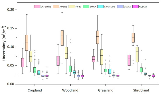
Figure 3.
Uncertainty of the seven SM products in different land cover types during 2015–2020. The black line in the box plot indicates the median value of uncertainty.
The high uncertainty of the AMSR2 product could be attributed to its poor retrieval precision globally, as revealed in previous studies [39,57]. For the FY-3C product, the median SM uncertainty was higher in woodland and shrubland than in cropland and grassland. This implies that the FY-3C SM is significantly influenced by vegetation, consistent with existing studies [58]. For the CCI-active product, a higher median uncertainty was observed primarily in grassland and shrubland. The median uncertainty of the SMAP product was higher in woodland than in other land cover types. SMAP is known to underestimate surface SM over densely vegetated areas due to biased surface temperature and other potential factors [59,60]. For the ERA5-Land product, there was no obvious difference in the median values of uncertainty across the four land cover types. The uncertainty of GLDAS and GLEAM products showed the best performance over all four land cover types, with both medians below 0.023 m3/m3. Moreover, the small amplitude in box variation suggests their stable performances over different land cover types. Considering the poor performances of AMSR2 and FY-3C, only the other five SM products were used in subsequent BTCH merging.
4.2. BTCH Merging
Figure 4 displays the Taylor diagram comparing BTCH-based, AVE-based, and five-parent SM products with in situ observations. As shown in this figure, the BTCH-based SM estimate outperformed these five-parent SM products with a significantly closer distance to in situ observations. This suggests that the BTCH merging method can effectively integrate the desirable characteristics of the original parent products and reduce unwanted random retrieval errors. Comparatively, the BTCH-based SM estimate also showed slightly better performance than the AVE-based SM estimate, providing full proof of the significance of weight optimization. In contrast to arithmetic average, the BTCH merging method assigns relatively high weights to pixels with low uncertainty, while high uncertainty indicates low weights. The arithmetic average method is only a special case that assumes the weights of multiple datasets to be equal; however, it rarely does so in practical applications.
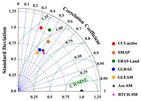
Figure 4.
Comparison of BTCH-based, AVE-based (the arithmetic average of five SM products), and five-parent SM products with in situ observations.
The relative weight (%) of each SM dataset has a key role in the BTCH merging method, as shown in Figure 5. In terms of weight values, the GLDAS product had the highest spatial-averaged weight (0.352), followed by GLEAM (0.284), then ERA5-Land (0.163), SMAP (0.139), and CCI-active (0.062). This is consistent with the uncertainty results in Figure 3, where products with low uncertainty are assigned high weight values and vice versa. Moreover, the merging weights varied among the parent products and showed large spatial variability. Specifically, the GLDAS SM product had relatively higher weights in the central and southeastern basin, while the GLEAM assigned high weights mainly in the northern and eastern basin. In contrast, the ERA5-Land and SMAP had high weights distributed in the southern and western basin, respectively. And the CCI-active displayed relatively lower weight over the entire basin. The regions with higher weight in each parent SM product mean that the merged SM over these parts will be more heavily weighted towards a particular parent SM product than the other products [61].
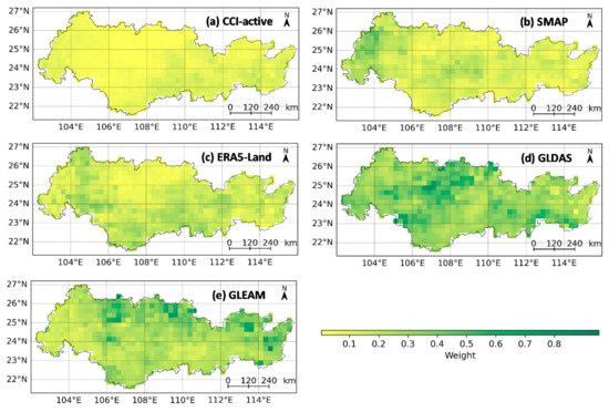
Figure 5.
The spatial distributions of merging weights for the five-parent SM products.
Furthermore, we evaluated the effect of SM uncertainty on the merged result, taking the 10 stations in the PRB on 1–5 April 2015 as an example. The SM uncertainty and the contribution of each SM product to the merged result were extracted at the station location, and their relevant relationship was examined, as shown in Figure 6. The contribution of each SM product to the merged result was quantified using , where is the merged SM. As shown in Figure 6, the SM uncertainty was obviously negatively correlated with its contribution to the merged result, i.e., the larger the SM uncertainty, the smaller its contribution to the merged result.
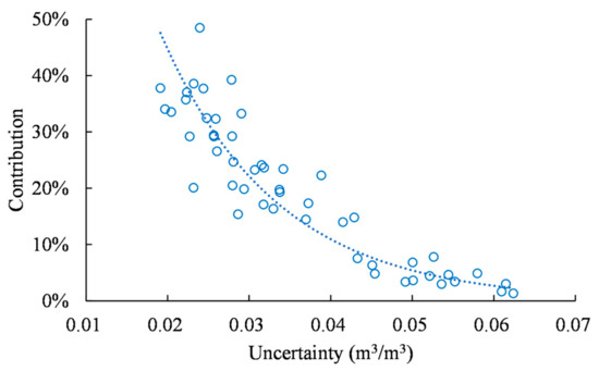
Figure 6.
Correlation between the SM uncertainty and its contribution to the merged result.
4.3. Spatial Downscaling of the Merged SM
4.3.1. Selection of Antecedent Precipitation Days
There is a delayed effect of meteorological factors on SM [62]. For precipitation, the SM condition on a specific day is not solely related to precipitation on that day; it may have a stronger correlation with the sliding cumulative value of precipitation from previous days, or even tens of days. Figure 7 illustrates the relationship between the sliding cumulative values of precipitation (antecedent precipitation ranging from 5 to 90 days) and SM from 2015 to 2020 in the PRB. It was observed that the antecedent precipitations ranging from 5 to 90 days were all significantly and positively related to SM, with the R curve first increasing rapidly and then decreasing slowly. The highest R value (0.530) was found between the 35-day sliding cumulative precipitation and SM. Therefore, an optimal time scale for the cumulative effect of precipitation on SM was set at 35 days in this paper.
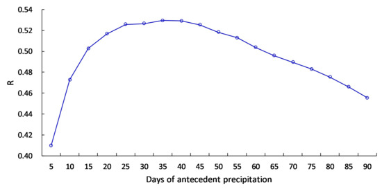
Figure 7.
Variation of R between the sliding cumulative values of precipitation and SM.
4.3.2. The Performance of Downscaling Models on the Test Dataset
Figure 8 shows scatterplots and statistical metrics of the RF-based and LSTM-based downscaling models on the 20% test dataset. In this paper, the RF and LSTM models without and with antecedent precipitation are referred to as RFpre, RFpre35, LSTMpre, and LSTMpre35, respectively. As indicated, the models with antecedent precipitation always outperformed the models without antecedent precipitation. That is, the scatterplot distributions for the RFpre35 and LSTMpre35 models (Figure 8b,d) were more concentrated than those for the RFpre and LSTMpre models (Figure 8a,c), also with large improvements in statistical metrics. For example, R2 increased by 10% and 12%, RMSE decreased by 14% and 17%, and MAE decreased by 14% and 18%, respectively. In addition, both the RFpre35 and LSTMpre35 models showed high consistency against the test dataset, with the LSTMpre35 model performing slightly better than the RFpre35 model. This suggested that the LSTMpre35 model can better learn the complex relationship between environmental variables and the target SM variable at a 0.25° spatial scale.
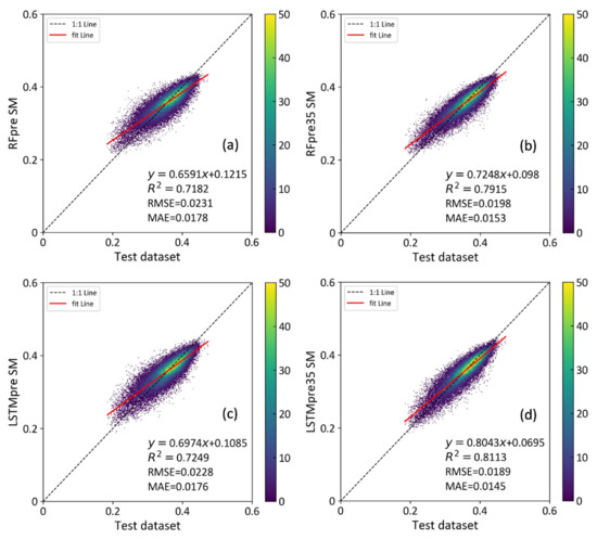
Figure 8.
Scatterplot of each downscaling model on test dataset (20%): (a,b) are RF models without and with antecedent precipitation; (c,d) are LSTM models without and with antecedent precipitation.
4.3.3. Spatial Distribution of the Downscaled SM
Figure 9 shows the spatial distributions of the original (merged) and downscaled SM (RFpre, RFpre35, LSTMpre, and LSTMpre35) on 1–5 April 2015. Compared to the original SM product (0.25°), the downscaled results at 0.05° resolution showed a significant improvement in spatial detail. Visually, the RFpre35 and LSTMpre35 downscaled SM maps better preserved the spatial patterns observed in the original SM data than the RFpre and LSTMpre maps. High SM values were generally found in the northeastern basin, while low values were observed in the central-western and some parts of the eastern basin. This indicates that antecedent precipitation plays a key role in influencing SM spatial distribution. Moreover, it is apparent that the RFpre35 downscaled SM map shows a smoothing effect, leading to underestimation of high values and overestimation of low values. In contrast, the LSTMpre35 downscaled SM map effectively reproduces the dynamic range of the original SM product, representing a large progress over other machine learning downscaling algorithms [30]. Thus, the LSTMpre35 downscaled result achieved the highest spatial consistency with the original SM product in the PRB.
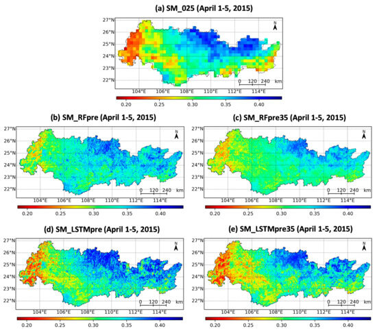
Figure 9.
Spatial distributions of the original (merged) and downscaled SM on 1–5 April 2015.
4.4. Validations of the Downscaled SM
4.4.1. Comparison with Ground Observations
Table 4 presents the statistical metrics of the original and downscaled SM against in situ observations. Compared to the original SM product, the downscaled results did not achieve favorable performance, with no significant improvement in the error statistics except for the average bias value. As shown, the original SM product had an average bias value of 0.034 m3/m3, while the downscaled SM had average bias values of 0.009~0.032 m3/m3.
Table 4.
Validation results of the original and downscaled SM against in situ observations. N represents the sample size.
Generally, the RFpre35 and LSTMpre35 downscaled results outperformed their respective counterparts, RFpre and LSTMpre. The R values at each station were higher, and the RMSE, MAE, and ubRMSE values were also smaller at most stations, with the same situation for the average metric values. In addition, the overestimation (average bias) of the LSTMpre and LSTMpre35 downscaling results was lower than that of the RFpre and RFpre35 results, respectively. Despite comparable accuracy performance, the LSTMpre35 downscaled result slightly outperformed the RFpre35 result, except for the average ubRMSE value with a difference of 0.002 m3/m3.
4.4.2. Comparison with CLDAS SM Data
The CLDAS SM data were employed as a reference to more fully evaluate the accuracy of the original and downscaled SM, as shown in Figure 10. To match the CLDAS SM data, the spatial resolution of both original and downscaled SM was resampled to 0.0625°. Considering the available CLDAS SM data, the time range for this section covers the period from 2017 to 2019.
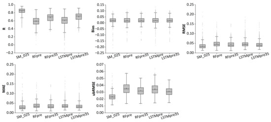
Figure 10.
Validation results of the original and downscaled SM against the CLDAS SM data.
Compared to the original SM product, the downscaled results did not show improved performance; however, they slightly reduced the overestimation. The original SM product had a median bias of 0.020 m3/m3, while the downscaled results had median biases of 0.017~0.019 m3/m3. Clearly, the downscaled SM results of RFpre35 and LSTMpre35 outperformed those of RFpre and LSTMpre, respectively. Moreover, the LSTMpre35 downscaled SM result (R = 0.719, Bias = 0.019 m3/m3, RMSE = 0.039 m3/m3, MAE = 0.030 m3/m3 and ubRMSE = 0.031 m3/m3) was superior to the RFpre35 result (R = 0.697, Bias = 0.017 m3/m3, RMSE = 0.040 m3/m3, MAE = 0.030 m3/m3 and ubRMSE = 0.032 m3/m3) in terms of the median metrics, although the difference was small. The above validation results were totally consistent with those against in situ observations.
4.5. Feature Importance Assessment
Figure 11 shows the importance of each explanatory feature from the RFpre35 downscaling model. It was found that pre35 predominated SM retrieval with the highest relative importance (30.01%), suggesting that antecedent precipitation played a significant role in reducing errors during model training. As a key variable directly causing SM changes, contemporary precipitation (pre) also showed high importance (15.76%), second only to pre35. The significance of pre35 and pre highlights that SM estimation is mainly influenced by precipitation, with antecedent precipitation having a greater impact than contemporary precipitation.
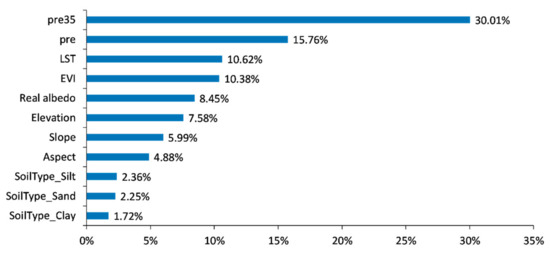
Figure 11.
Feature importance ranking from the RFpre35 downscaling model.
LST was also identified as a critical variable (10.62%) due to the controlling effect of surface SM on surface energy exchange and partitioning [2]. Vegetation index and albedo are commonly used to describe SM variations in triangular/trapezoidal methods because of their ability to reflect vegetation status and surface energy fluxes [63]. In this study, EVI was used to avoid the problem of vegetation saturation. As expected, EVI and real surface albedo showed relatively high importance with 10.38% and 8.45%, respectively. Among three topographic factors, elevation was found to be the most important (7.58%), followed by slope (5.99%) and aspect (4.88%). This indicates a greater influence of elevation on SM over regions with large height differences (about 3000 m in the PRB). In addition, soil texture presented 1–3% importance for sand, silt, and clay, respectively, due to the strong influence of these properties on water infiltration rates, permeability, and soil water storage capacity [8]. It is noted that a lower ranking does not necessarily mean that a feature is unimportant, as the SM estimation of the downscaling model is based on a combined judgement of all input variables.
5. Discussion
5.1. Advantages and Limitations in the BTCH Method
Although the TCH-based uncertainty may underestimate the absolute uncertainty as compared to gauge-based validation, the relative uncertainty among individual products can be well retained [17]. Based on Figure 3 and Figure 4, five SM products were merged using the BTCH method, and the BTCH-based SM estimate demonstrated superior performance to the five parent products and the AVE-based SM estimate. The advantages of the BTCH merging in uncertainty reduction and weight optimization were also reported in previous studies regarding other geographic elements, such as gross primary productivity [18] and terrestrial evapotranspiration [19].
It is known that SM contains spatio-temporal non-stationary random errors that may be stationary in one dimension but non-stationary in another [64]. The TCH method assumed that the errors of SM data were static and time-invariant, failing to fully characterize the error information of SM, especially in time domain [9]. There are some studies that consider the spatio-temporal non-stationary errors in TC-based merging [64,65,66]; however, there are fewer in TCH-based merging. It would make sense to fill and enrich this gap in further studies.
5.2. Importance of Antecedent Precipitation
The choice of the length of the antecedent precipitation depends on study area characteristics. The period of antecedent precipitation deemed significant in previous studies varies considerably, ranging from 10 to 90 days [32,33,67,68]. For example, Schoener et al. [67] proposed a new approach for estimating catchment-scale SM using an antecedent precipitation index (API)-based model, in which an antecedent period of 13 days was determined through a sensitivity analysis. Liu et al. [33] developed a linear regression model that links antecedent effective precipitation and SM, using a 90-day antecedent period. The model achieved an accuracy rate of over 93% when applied to monitor autumn and winter drought in certain areas of Hubei in 2007. These studies showed that considering antecedent precipitation on an appropriate timescale is essential for accurate estimation and effective application of SM.
In this paper, the optimal time scale for the cumulative effect of precipitation on SM was set at 35 days. The comparison of downscaling models (Figure 8, Figure 9 and Figure 10 and Table 4) revealed that the models with antecedent precipitation obtained significantly better performance, demonstrating their strong stabilities in estimating SM at both temporal and spatial scales. This result was reasonably explained by the feature importance ranking in Figure 11, which showed the highest contribution (30.01%) of antecedent precipitation in the study region.
Moreover, this study determined the optimal time scale (35 days) for the cumulative effect of precipitation on SM in the entire PRB throughout the whole study period. However, the effect of precipitation on SM is highly variable both in temporal and spatial domains. In terms of temporal scale, other temporal dynamics that may affect SM (e.g., seasonal variability and wet/dry seasons, or lag effects beyond the 35-day window) should also be explored in future research. In terms of spatial scale, different areas should be delineated to better characterize the relationship between precipitation and SM, especially in a large area encompassing several climatic zones and different topographies.
5.3. Uncertainty in the Validation of Downscaled SM
According to the validation results in Table 4 and Figure 10, the downscaled SM did not show better performances than the original SM product. Other studies have reported similar decreases in accuracy after downscaling [26,28], even when the downscaled SM was compared with sufficient ground measurements. It is challenging for the regressed SM (the downscaled SM at 0.05°) to transcend the original SM product (the merged SM at 0.25°) in data accuracy because the original SM data (80% of the data) were employed as a training sample for model building [28,69,70]. It should be noted that the predictive range of SM is restricted to those covered by the training data. Thus, the capability of downscaling models to reproduce SM at a finer scale is closely related to the moisture contrasts in the training data. As the bottleneck factor of precision restriction, the quality of the original SM product needed to be improved, such as the BTCH merging used in this study. There are also other ways to improve the quality of the original merged SM product, e.g., improving the quality of SM products involved in the merging process, or using alternative merging methods that take into account the inherent error of SM products. For satellite SM products, the improvement of retrieval algorithms and sufficient in situ measurement-based correction would be effective ways. Model-based SM products could be further refined by improved quality of meteorological forcing data and the soil property database. Moreover, other merging methods that considered the inherent error of SM products, such as Bayesian model averaging [71], data assimilation based on Kalman filtering [72], and optimal interpolation [73], should be applied to compare with the BTCH approach in future studies.
Moreover, the statistical metrics calculated in Table 4 are inevitably influenced by many factors, such as the limited number of in situ stations; the depth difference between the merged and downscaled SM (0–5 cm) and in situ SM (10 cm); and the spatial scale difference between the merged SM (0.25°), in situ SM (point scale), and the downscaled SM (0.05°). There was always unreasonable spatial matching when verifying remote sensing or model-based SM products with ground measurements. To address this issue, alternative methods were required, such as the CLDAS SM data used in this study or other SM-related physical elements that may be employed in future studies. Moreover, more robust methods, e.g., geostatistical approaches, regional-scale validation [57], and higher-density ground networks that are spatially representative, could also mitigate these issues. For example, Wang et al. [74] proposed a model-based geostatistical approach to upscale ground-based SM observations of unequal precision, and they successfully verified this approach in the Heihe Watershed Allied Telemetry Experimental Research experiment.
5.4. Limitations and Future Directions of Machine/Deep Learning Model
Machine/deep-learning-based models with transfer learning capabilities should be developed in the future for SM estimation. Note that transferability without additional training over a new location’s data has remained a significant challenge for all machine/deep learning models. This would involve applying the model to a diverse range of environments, from arid to tropical regions, and from flat plains to mountainous terrains. Yang et al. [75] proposed a Climate-Adaptive Transfer Learning (CATL) framework to improve SM estimation for a data scarce region, the Qinghai–Tibet Plateau (QTP). Specifically, regarding the QTP as the target region, selecting the areas with similar climate types with QTP as the source region, they train the machine/deep learning model in the source region and then transfer it to the target region via fine-tuning strategy. Results indicate that the CATL framework significantly improved the SM estimation in the QTP, achieving better precision.
Machine/deep-learning-based models with physical interpretation should be developed in the future for SM estimation. While machine/deep-learning-based models have shown superior efficiency and accuracy in our study and others, they are often criticized due to problems of overfitting and lack of physical understanding and explainability. Recently, Singh and Gaurav [76] proposed a learning bias physics-informed machine learning (PIML) model to estimate surface SM, incorporating the physics in the loss function of a fully connected feed-forward neural network (FFNN). Similarly, Chavoshi et al. [77] proposed a physics-informed neural networks (PINN) model that estimates the vadose zone soil water content (VZSWC) profile by incorporating Richardson’s equation as its primary physical constraint, and it achieved satisfactory performances. Both PIML-SM and PINN-SM models demonstrated that models that can effectively bridge the gap between data-driven models, and physical understanding will be the future development trend in environmental modelling applications.
6. Conclusions
This paper developed a two-step SM reconstruction approach, combining the BTCH merging and machine/deep-learning downscaling algorithms to generate a high-quality and high-spatial-resolution (0.05°) pentad SM dataset from microwave and model-based SM products. The reconstruction approach was tested over the PRB, and the performance of the obtained merged and downscaled SM results was fully assessed, with the main conclusions as below:
- (1)
- During 2015–2020, the TCH-based uncertainty ranking of seven SM products on four main land cover types in the PRB was consistent: (GLDAS and GLEAM) < ERA5-Land < SMAP < CCI-active < FY-3C < AMSR2. Moreover, the BTCH-based SM estimate outperformed five parent products and the AVE-based SM estimate, indicating that BTCH is a fusion approach that can effectively reduce data uncertainties and optimize weights.
- (2)
- The optimal time scale for the cumulative effect of precipitation on SM is 35 days for the period from 2015 to 2020 in the PRB. Validation on the 20% test dataset, visual comparison on spatial distributions, and validation against in situ observations and the CLDAS SM data all showed that adding an antecedent precipitation variable as a predictor can greatly improve the performance of SM downscaling models, both at the 0.25° and 0.05° spatial scales. The feature importance assessment also revealed that precipitation is a key variable to our SM downscaling models, with a greater influence of antecedent precipitation (30.01%) than contemporary precipitation (15.76%). Moreover, the LSTMpre35 model performed slightly better than the RFpre35 model.
- (3)
- Validation against in situ observations and the CLDAS SM data also indicated that the downscaled SM results were mainly limited by the original SM data in terms of data accuracy and were difficult to surpass. However, they did alleviate the overestimation inherent in the original SM data.
In conclusion, the two-step SM reconstruction approach has great potential in generating a high-quality and high-spatial-resolution SM dataset and could act as a reference for SM studies in other areas or for other earth science variables. Future works will investigate the potential of the obtained SM dataset in drought monitoring or other hydrological applications.
Author Contributions
Conceptualization, methodology, software, validation, data curation, writing—original draft preparation, writing—review and editing, visualization, Y.Z.; conceptualization, supervision, funding acquisition, Y.C.; writing—review and editing, visualization, L.C. All authors have read and agreed to the published version of the manuscript.
Funding
This study was supported by the Natural Science Foundation of China (Grant No. U2243227).
Data Availability Statement
CCI-active product can be obtained at https://www.esa-soilmoisture-cci.org/. AMSR2 product can be obtained at https://search.earthdata.nasa.gov/search. FY-3C product can be obtained at http://satellite.nsmc.org.cn/DataPortal/cn/home/index.html. SMAP product can be obtained at https://nsidc.org/data/smap/data. ERA5-Land product can be obtained at https://cds.climate.copernicus.eu/datasets. GLDAS product can be obtained at https://disc.gsfc.nasa.gov/datasets/GLDAS_NOAH025_3H_2.1/summary?keywords=GLDAS. GLEAM product can be obtained at https://www.gleam.eu/. CLDAS product can be obtained at http://data.cma.cn/data/. GlobeLand30 is available at https://www.webmap.cn/commres.do?method=globeIndex. CHIRPS precipitation data are available at https://data.chc.ucsb.edu/products/. LST data are available at http://data.tpdc.ac.cn/en/data/b8c448ab-9c50-43fe-9b5d-2a5888658fe6/. MODIS data can be accessed at https://search.earthdata.nasa.gov/. SRTM is available at https://srtm.csi.cgiar.org/srtmdata/. HWSD is available at https://www.fao.org/soils-portal/soil-survey/soil-maps-and-databases/harmonized-world-soil-database-v12/en/. All the above data were accessed on 20 January 2025.
Acknowledgments
The authors would like to thank the reviewers and the handling editor whose comments and suggestions improved this paper.
Conflicts of Interest
The authors declare no conflicts of interest.
References
- McColl, K.A.; Alemohammad, S.H.; Akbar, R.; Konings, A.G.; Yueh, S.; Entekhabi, D. The global distribution and dynamics of surface soil moisture. Nat. Geosci. 2017, 10, 100–104. [Google Scholar] [CrossRef]
- Long, D.; Bai, L.; Yan, L.; Zhang, C.; Yang, W.; Lei, H.; Quan, J.; Meng, X.; Shi, C. Generation of spatially complete and daily continuous surface soil moisture of high spatial resolution. Remote Sens. Environ. 2019, 233, 111364. [Google Scholar] [CrossRef]
- Brocca, L.; Melone, F.; Moramarco, T.; Wagner, W.; Naeimi, V.; Bartalis, Z.; Hasenauer, S. Improving runoff prediction through the assimilation of the ASCAT soil moisture product. Hydrol. Earth Syst. Sci. 2010, 14, 1881–1893. [Google Scholar] [CrossRef]
- Sehgal, V.; Gaur, N.; Mohanty, B.P. Global Flash Drought Monitoring Using Surface Soil Moisture. Water Resour. Res. 2021, 57, e2021WR029901. [Google Scholar] [CrossRef]
- Borodychev, V.V.; Lytov, M.N. Irrigation management model based on soil moisture distribution profile. IOP Conf. Ser. Earth Environ. Sci. 2020, 577, 012022. [Google Scholar] [CrossRef]
- Dobriyal, P.; Qureshi, A.; Badola, R.; Hussain, S.A. A review of the methods available for estimating soil moisture and its implications for water resource management. J. Hydrol. 2012, 458–459, 110–117. [Google Scholar] [CrossRef]
- Crow, W.T.; Berg, A.A.; Cosh, M.H.; Loew, A.; Mohanty, B.P.; Panciera, R.; de Rosnay, P.; Ryu, D.; Walker, J.P. Upscaling sparse ground-based soil moisture observations for the validation of coarse-resolution satellite soil moisture products. Rev. Geophys. 2012, 50, RG2002. [Google Scholar] [CrossRef]
- Zhang, Y.; Chen, Y.; Chen, L.; Xu, S.; Sun, H. A machine learning-based approach for generating high-resolution soil moisture from SMAP products. Geocarto Int. 2022, 37, 16086–16107. [Google Scholar] [CrossRef]
- Shangguan, Y.L.; Min, X.X.; Shi, Z. Inter-comparison and integration of different soil moisture downscaling methods over the Qinghai-Tibet Plateau. J. Hydrol. 2023, 617, 129014. [Google Scholar] [CrossRef]
- Ming, W.; Ji, X.; Zhang, M.; Li, Y.; Liu, C.; Wang, Y.; Li, J. A Hybrid Triple Collocation-Deep Learning Approach for Improving Soil Moisture Estimation from Satellite and Model-Based Data. Remote Sens. 2022, 14, 1744. [Google Scholar] [CrossRef]
- Wood, E.F.; Roundy, J.K.; Troy, T.J.; van Beek, L.P.H.; Bierkens, M.F.P.; Blyth, E.; de Roo, A.; Döll, P.; Ek, M.; Famiglietti, J.; et al. Hyperresolution global land surface modeling: Meeting a grand challenge for monitoring Earth’s terrestrial water. Water Resour. Res. 2011, 47, W05301. [Google Scholar] [CrossRef]
- Min, X.; Shangguan, Y.; Li, D.; Shi, Z. Improving the fusion of global soil moisture datasets from SMAP, SMOS, ASCAT, and MERRA2 by considering the non-zero error covariance. Int. J. Appl. Earth Obs. Geoinf. 2022, 113, 103016. [Google Scholar] [CrossRef]
- Xie, Q.X.; Jia, L.; Menenti, M.; Hu, G.C. Global soil moisture data fusion by Triple Collocation Analysis from 2011 to 2018. Sci. Data 2022, 9, 687. [Google Scholar] [CrossRef]
- Kim, S.; Pham, H.T.; Liu, Y.Y.; Marshall, L.; Sharma, A. Improving the Combination of Satellite Soil Moisture Data Sets by Considering Error Cross Correlation: A Comparison Between Triple Collocation (TC) and Extended Double Instrumental Variable (EIVD) Alternatives. IEEE Trans. Geosci. Remote Sens. 2021, 59, 7285–7295. [Google Scholar] [CrossRef]
- Stoffelen, A. Toward the true near-surface wind speed: Error modeling and calibration using triple collocation. J. Geophys. Res. Ocean. 1998, 103, 7755–7766. [Google Scholar] [CrossRef]
- Premoli, A.; Tavella, P. A revisited three-cornered hat method for estimating frequency standard instability. IEEE Trans. Instrum. Meas. 1993, 42, 7–13. [Google Scholar] [CrossRef]
- Xu, L.; Chen, N.C.; Moradkhani, H.; Zhang, X.; Hu, C.L. Improving Global Monthly and Daily Precipitation Estimation by Fusing Gauge Observations, Remote Sensing, and Reanalysis Data Sets. Water Resour. Res. 2020, 56, e2019WR026444. [Google Scholar] [CrossRef]
- Zhang, Y.H.; Ye, A.Z. Improving global gross primary productivity estimation by fusing multi-source data products. Heliyon 2022, 8, e09153. [Google Scholar] [CrossRef]
- He, X.; Xu, T.; Xia, Y.; Bateni, S.M.; Guo, Z.; Liu, S.; Mao, K.; Zhang, Y.; Feng, H.; Zhao, J. A Bayesian Three-Cornered Hat (BTCH) Method: Improving the Terrestrial Evapotranspiration Estimation. Remote Sens. 2020, 12, 878. [Google Scholar] [CrossRef]
- Liu, J.; Chai, L.N.; Dong, J.Z.; Zheng, D.H.; Wigneron, J.P.; Liu, S.M.; Zhou, J.; Xu, T.R.; Yang, S.Q.; Song, Y.Z.; et al. Uncertainty analysis of eleven multisource soil moisture products in the third pole environment based on the three-corned hat method. Remote Sens. Environ. 2021, 255, 112225. [Google Scholar] [CrossRef]
- Kim, H.; Wigneron, J.-P.; Kumar, S.; Dong, J.; Wagner, W.; Cosh, M.H.; Bosch, D.D.; Collins, C.H.; Starks, P.J.; Seyfried, M.; et al. Global scale error assessments of soil moisture estimates from microwave-based active and passive satellites and land surface models over forest and mixed irrigated/dryland agriculture regions. Remote Sens. Environ. 2020, 251, 112052. [Google Scholar] [CrossRef]
- Chauhan, N.S.; Miller, S.; Ardanuy, P. Spaceborne soil moisture estimation at high resolution: A microwave-optical/IR synergistic approach. Int. J. Remote Sens. 2003, 24, 4599–4622. [Google Scholar] [CrossRef]
- Merlin, O.; Rudiger, C.; Al Bitar, A.; Richaume, P.; Walker, J.P.; Kerr, Y.H. Disaggregation of SMOS Soil Moisture in Southeastern Australia. IEEE Trans. Geosci. Remote Sens. 2012, 50, 1556–1571. [Google Scholar] [CrossRef]
- Carlson, T.N.; Gillies, R.R.; Perry, E.M. A method to make use of thermal infrared temperature and NDVI measurements to infer surface soil water content and fractional vegetation cover. Remote Sens. Rev. 1994, 9, 161–173. [Google Scholar] [CrossRef]
- Peng, J.; Loew, A.; Merlin, O.; Verhoest, N.E.C. A review of spatial downscaling of satellite remotely sensed soil moisture. Rev. Geophys. 2017, 55, 341–366. [Google Scholar] [CrossRef]
- Mao, T.N.; Shangguan, W.; Li, Q.L.; Li, L.; Zhang, Y.; Huang, F.N.; Li, J.D.; Liu, W.; Zhang, R.Q. A Spatial Downscaling Method for Remote Sensing Soil Moisture Based on Random Forest Considering Soil Moisture Memory and Mass Conservation. Remote Sens. 2022, 14, 3858. [Google Scholar] [CrossRef]
- Xu, W.; Zhang, Z.; Long, Z.; Qin, Q. Downscaling SMAP Soil Moisture Products With Convolutional Neural Network. IEEE J. Sel. Top. Appl. Earth Obs. Remote Sens. 2021, 14, 4051–4062. [Google Scholar] [CrossRef]
- Liu, Y.; Jing, W.; Wang, Q.; Xia, X. Generating high-resolution daily soil moisture by using spatial downscaling techniques: A comparison of six machine learning algorithms. Adv. Water Resour. 2020, 141, 103601. [Google Scholar] [CrossRef]
- Song, C.Y.; Jia, L.; Menenti, M. Retrieving High-Resolution Surface Soil Moisture by Downscaling AMSR-E Brightness Temperature Using MODIS LST and NDVI Data. IEEE J. Sel. Top. Appl. Earth Obs. Remote Sens. 2014, 7, 935–942. [Google Scholar] [CrossRef]
- Wei, Z.; Meng, Y.; Zhang, W.; Peng, J.; Meng, L. Downscaling SMAP soil moisture estimation with gradient boosting decision tree regression over the Tibetan Plateau. Remote Sens. Environ. 2019, 225, 30–44. [Google Scholar] [CrossRef]
- Yan, R.; Bai, J. A New Approach for Soil Moisture Downscaling in the Presence of Seasonal Difference. Remote Sens. 2020, 12, 2818. [Google Scholar] [CrossRef]
- Zhao, Y.; Wei, F.; Yang, H.; Jiang, Y. Discussion on Using Antecedent Precipitation Index to Supplement Relative Soil Moisture Data Series. Procedia Environ. Sci. 2011, 10, 1489–1495. [Google Scholar] [CrossRef]
- Liu, K.; Liu, Z.; Liang, Y.; Wan, S.; Tan, Y. Method for Soil Moisture Calculation in Plough Layer Based on Antecedent Effective Rainfall. Chin. J. Agrometeorol. 2009, 30, 365–369. (In Chinese) [Google Scholar]
- Zhang, T.; Chen, Y. Analysis of Dynamic Spatiotemporal Changes in Actual Evapotranspiration and Its Associated Factors in the Pearl River Basin Based on MOD16. Water 2017, 9, 832. [Google Scholar] [CrossRef]
- Dorigo, W.A.; Gruber, A.; De Jeu, R.A.M.; Wagner, W.; Stacke, T.; Loew, A.; Albergel, C.; Brocca, L.; Chung, D.; Parinussa, R.M.; et al. Evaluation of the ESA CCI soil moisture product using ground-based observations. Remote Sens. Environ. 2015, 162, 380–395. [Google Scholar] [CrossRef]
- Parinussa, R.M.; Holmes, T.R.H.; Wanders, N.; Dorigo, W.A.; de Jeu, R.A.M. A Preliminary Study toward Consistent Soil Moisture from AMSR2. J. Hydrometeorol. 2015, 16, 932–947. [Google Scholar] [CrossRef]
- Zhu, Y.C.; Li, X.; Pearson, S.; Wu, D.L.; Sun, R.J.; Johnson, S.; Wheeler, J.; Fang, S.B. Evaluation of Fengyun-3C Soil Moisture Products Using In-Situ Data from the Chinese Automatic Soil Moisture Observation Stations: A Case Study in Henan Province, China. Water 2019, 11, 248. [Google Scholar] [CrossRef]
- Entekhabi, D.; Njoku, E.G.; Neill, P.E.O.; Kellogg, K.H.; Crow, W.T.; Edelstein, W.N.; Entin, J.K.; Goodman, S.D.; Jackson, T.J.; Johnson, J.; et al. The Soil Moisture Active Passive (SMAP) Mission. Proc. IEEE 2010, 98, 704–716. [Google Scholar] [CrossRef]
- Ma, H.L.; Zeng, J.Y.; Chen, N.C.; Zhang, X.; Cosh, M.H.; Wang, W. Satellite surface soil moisture from SMAP, SMOS, AMSR2 and ESA CCI: A comprehensive assessment using global ground-based observations. Remote Sens. Environ. 2019, 231, 111215. [Google Scholar] [CrossRef]
- Munoz-Sabater, J.; Dutra, E.; Agusti-Panareda, A.; Albergel, C.; Arduini, G.; Balsamo, G.; Boussetta, S.; Choulga, M.; Harrigan, S.; Hersbach, H.; et al. ERA5-Land: A state-of-the-art global reanalysis dataset for land applications. Earth Syst. Sci. Data 2021, 13, 4349–4383. [Google Scholar] [CrossRef]
- Rodell, M.; Houser, P.R.; Jambor, U.; Gottschalck, J.; Mitchell, K.; Meng, C.J.; Arsenault, K.; Cosgrove, B.; Radakovich, J.; Bosilovich, M.; et al. The global land data assimilation system. Bull. Am. Meteorol. Soc. 2004, 85, 381–394. [Google Scholar] [CrossRef]
- Martens, B.; Miralles, D.G.; Lievens, H.; van der Schalie, R.; de Jeu, R.A.M.; Fernandez-Prieto, D.; Beck, H.E.; Dorigo, W.A.; Verhoest, N.E.C. GLEAM v3: Satellite-based land evaporation and root-zone soil moisture. Geosci. Model Dev. 2017, 10, 1903–1925. [Google Scholar] [CrossRef]
- Shi, C.X.; Xie, Z.H.; Qian, H.; Liang, M.L.; Yang, X.C. China land soil moisture EnKF data assimilation based on satellite remote sensing data. Sci. China Earth Sci. 2011, 54, 1430–1440. [Google Scholar] [CrossRef]
- Chen, J.; Ban, Y.; Li, S. Open access to Earth land-cover map. Nature 2014, 514, 434. [Google Scholar] [CrossRef]
- Zhao, T.; Yu, P. Global Daily 0.05° Spatiotemporal Continuous Land Surface Temperature Dataset (2002–2022); National Tibetan Plateau/Third Pole Environment Data Center: Beijing, China, 2021. [Google Scholar] [CrossRef]
- Chen, J.; Jönsson, P.; Tamura, M.; Gu, Z.; Matsushita, B.; Eklundh, L. A simple method for reconstructing a high-quality NDVI time-series data set based on the Savitzky–Golay filter. Remote Sens. Environ. 2004, 91, 332–344. [Google Scholar] [CrossRef]
- Govaerts, Y.; Dickinson, R.E.; Widlowski, J.-L.; Taberner, M.; Gobron, N.; Verstraete, M.M.; Martonchik, J.V.; Lattanzio, A.; Pinty, B. Coupling Diffuse Sky Radiation and Surface Albedo. J. Atmos. Sci. 2005, 62, 2580–2591. [Google Scholar] [CrossRef]
- Farr, T.G.; Rosen, P.A.; Caro, E.; Crippen, R.; Duren, R.; Hensley, S.; Kobrick, M.; Paller, M.; Rodriguez, E.; Roth, L.; et al. The Shuttle Radar Topography Mission. Rev. Geophys. 2007, 45, RG2004. [Google Scholar] [CrossRef]
- Nachtergaele, F.O.; Velthuizen, H.v.; Verelst, L.; Wiberg, D.; Batjes, N.H.; Dijkshoorn, J.A.; Engelen, V.W.P.v.; Fischer, G.; Jones, A.; Montanarella, L.; et al. Harmonized World Soil Database; Version 1.2; Joint Research Centre of the EC: Laxenburg, Austria, 2012. [Google Scholar]
- Western, A.W.; Grayson, R.B.; Blöschl, G. Scaling of Soil Moisture: A Hydrologic Perspective. Annu. Rev. Earth Planet. Sci. 2002, 30, 149–180. [Google Scholar] [CrossRef]
- Ferreira, V.G.; Montecino, H.D.C.; Yakubu, C.I.; Heck, B. Uncertainties of the Gravity Recovery and Climate Experiment time-variable gravity-field solutions based on three-cornered hat method. J. Appl. Remote Sens. 2016, 10, 015015. [Google Scholar] [CrossRef]
- Galindo, F.J.; Palacio, J. Estimating the instabilities of N correlated clocks. In Proceedings of the 31th Annual Precise Time and Time Interval Systems and Applications Meeting, Dana Point, CA, USA, 7–9 December 1999; pp. 285–296. [Google Scholar]
- Abbaszadeh, P.; Moradkhani, H.; Zhan, X. Downscaling SMAP Radiometer Soil Moisture Over the CONUS Using an Ensemble Learning Method. Water Resour. Res. 2019, 55, 324–344. [Google Scholar] [CrossRef]
- Breiman, L. Random Forests. Mach. Learn. 2001, 45, 5–32. [Google Scholar] [CrossRef]
- Hochreiter, S.; Schmidhuber, J. Long Short-Term Memory. Neural Comput. 1997, 9, 1735–1780. [Google Scholar] [CrossRef] [PubMed]
- Srivastava, N.; Hinton, G.; Krizhevsky, A.; Sutskever, I.; Salakhutdinov, R. Dropout: A Simple Way to Prevent Neural Networks from Overfitting. J. Mach. Learn. Res. 2014, 15, 1929–1958. [Google Scholar]
- Zheng, J.Y.; Zhao, T.J.; Lu, H.S.; Shi, J.C.; Cosh, M.H.; Ji, D.B.; Jiang, L.M.; Cui, Q.; Lu, H.; Yang, K.; et al. Assessment of 24 soil moisture datasets using a new in situ network in the Shandian River Basin of China. Remote Sens. Environ. 2022, 271, 112891. [Google Scholar] [CrossRef]
- Fan, Y.; Qiu, J.; Dong, J.; Zhang, X.H.; Dagang, W. Error Characteristics of Microwave Soil Moisture Products based on Triple Collocation and Its Spatial-temporal Pattern. Remote Sens. Technol. Appl. 2020, 35, 85–96. (In Chinese) [Google Scholar]
- Fan, X.W.; Liu, Y.B.; Gan, G.J.; Wu, G.P. SMAP underestimates soil moisture in vegetation-disturbed areas primarily as a result of biased surface temperature data. Remote Sens. Environ. 2020, 247, 111914. [Google Scholar] [CrossRef]
- Xu, L.; Chen, N.C.; Zhang, X.; Moradkhani, H.; Zhang, C.; Hu, C.L. In-situ and triple-collocation based evaluations of eight global root zone soil moisture products. Remote Sens. Environ. 2021, 254, 112248. [Google Scholar] [CrossRef]
- Peng, J.; Tanguy, M.; Robinson, E.L.; Pinnington, E.; Evans, J.; Ellis, R.; Cooper, E.; Hannaford, J.; Blyth, E.; Dadson, S. Estimation and evaluation of high-resolution soil moisture from merged model and Earth observation data in the Great Britain. Remote Sens. Environ. 2021, 264, 112610. [Google Scholar] [CrossRef]
- Yuan, S.; He, X.; Gu, X.; Pan, T.; Yu, F. Response of Declining Soil Moisture on Meteorological Factors over Karst Area of Guizhou Province. Chin. J. Soil Sci. 2018, 49, 320–328. (In Chinese) [Google Scholar] [CrossRef]
- Park, S.; Im, J.; Park, S.; Rhee, J. Drought monitoring using high resolution soil moisture through multi-sensor satellite data fusion over the Korean peninsula. Agric. For. Meteorol. 2017, 237–238, 257–269. [Google Scholar] [CrossRef]
- Zhou, J.H.; Crow, W.T.; Wu, Z.Y.; Dong, J.Z.; He, H.; Feng, H.H. A triple collocation-based 2D soil moisture merging methodology considering spatial and temporal non-stationary errors. Remote Sens. Environ. 2021, 263, 112509. [Google Scholar] [CrossRef]
- Wu, K.; Ryu, D.; Nie, L.; Shu, H. Time-variant error characterization of SMAP and ASCAT soil moisture using Triple Collocation Analysis. Remote Sens. Environ. 2021, 256, 112324. [Google Scholar] [CrossRef]
- Shangguan, Y.; Min, X.; Wang, N.; Tong, C.; Shi, Z. A long-term, high-accuracy and seamless 1km soil moisture dataset over the Qinghai-Tibet Plateau during 2001–2020 based on a two-step downscaling method. GIScience Remote Sens. 2024, 61, 2290337. [Google Scholar] [CrossRef]
- Schoener, G.; Stone, M.C. Monitoring soil moisture at the catchment scale—A novel approach combining antecedent precipitation index and radar-derived rainfall data. J. Hydrol. 2020, 589, 125155. [Google Scholar] [CrossRef]
- Zhao, B.; Dai, Q.; Han, D.; Dai, H.; Mao, J.; Zhuo, L.; Rong, G. Estimation of soil moisture using modified antecedent precipitation index with application in landslide predictions. Landslides 2019, 16, 2381–2393. [Google Scholar] [CrossRef]
- Hutengs, C.; Vohland, M. Downscaling land surface temperatures at regional scales with random forest regression. Remote Sens. Environ. 2016, 178, 127–141. [Google Scholar] [CrossRef]
- Zeng, L.; Hu, S.; Xiang, D.; Zhang, X.; Li, D.; Li, L.; Zhang, T. Multilayer Soil Moisture Mapping at a Regional Scale from Multisource Data via a Machine Learning Method. Remote Sens. 2019, 11, 284. [Google Scholar] [CrossRef]
- Kim, J.; Mohanty, B.P.; Shin, Y. Effective soil moisture estimate and its uncertainty using multimodel simulation based on Bayesian Model Averaging. J. Geophys. Res.-Atmos. 2015, 120, 8023–8042. [Google Scholar] [CrossRef]
- Reichle, R.H.; Crow, W.T.; Keppenne, C.L. An adaptive ensemble Kalman filter for soil moisture data assimilation. Water Resour. Res. 2008, 44, W03423. [Google Scholar] [CrossRef]
- Jiang, L.; Shi, C.; Sun, S.; Liang, X. Fusion of In-Situ Soil Moisture and Land Surface Model Estimates Using Localized Ensemble Optimum Interpolation over China. J. Meteorol. Res. 2020, 34, 1335–1346. [Google Scholar] [CrossRef]
- Wang, J.; Ge, Y.; Song, Y.; Li, X. A Geostatistical Approach to Upscale Soil Moisture With Unequal Precision Observations. IEEE Geosci. Remote Sens. Lett. 2014, 11, 2125–2129. [Google Scholar] [CrossRef]
- Yang, J.; Yang, Q.; Hu, F.; Shao, J.; Wang, G. A climate-adaptive transfer learning framework for improving soil moisture estimation in the Qinghai-Tibet Plateau. J. Hydrol. 2024, 630, 130717. [Google Scholar] [CrossRef]
- Singh, A.; Gaurav, K. PIML-SM: Physics-Informed Machine Learning to Estimate Surface Soil Moisture From Multisensor Satellite Images by Leveraging Swarm Intelligence. IEEE Trans. Geosci. Remote Sens. 2024, 62, 1–13. [Google Scholar] [CrossRef]
- Chavoshi, A.; Dashtian, H.; Bakhshian, S.; Young, M.H.; Niyogi, D. PINN-SM: A Physics-Informed Neural Networks Model for Vadose Zone Soil Moisture Profile Prediction. arXiv 2024. [Google Scholar] [CrossRef]
Disclaimer/Publisher’s Note: The statements, opinions and data contained in all publications are solely those of the individual author(s) and contributor(s) and not of MDPI and/or the editor(s). MDPI and/or the editor(s) disclaim responsibility for any injury to people or property resulting from any ideas, methods, instructions or products referred to in the content. |
© 2025 by the authors. Licensee MDPI, Basel, Switzerland. This article is an open access article distributed under the terms and conditions of the Creative Commons Attribution (CC BY) license (https://creativecommons.org/licenses/by/4.0/).