Probabilistic Risk Assessment (PRA) for Sustainable Water Resource Management: A Future Flood Inundation Example

Abstract

Sustainable decision making addresses resource and cost sharing among current and future generations. Adaptation costs are incurred by current and damage mitigation costs are borne by future generations. Circularity extends sustainability by including resource regeneration and benefits from resource re-use. Climate change and associated global warming are producing more frequent extreme events with different probabilities of occurrence than historically observed. Traditional approaches to asset and infrastructure design tend to be backward-looking for weather- and climate-related bases and to introduce too little variability to compensate for uncertainty, resulting in infrastructure that was designed for irrelevant future conditions. An example dynamic probabilistic risk assessment (PRA) for flood inundation is developed and implemented to examine the usefulness and limitations of PRA for sustainable water resource management. It specifically addresses the issue of sustainable decision making related to outdated but historically regulatory-compliant assets under non-stationary climatic conditions. Weather attribution provides improved extreme event frequency expectations to, generates the dynamic component of, and allows for incorporation of additional uncertainty to the PRA. Results from the PRA provide decision making optimization between current adaptation and future mitigation costs. A limitation of PRA is that it analyzes failure and risk and not benefits accruing from resource regeneration.

1. Introduction

Sustainability can be defined as meeting the needs of the present without compromising the ability of future generations to meet their needs [1,2,3]. Inherent in the concept of sustainability is the rationed exploitation and communal management of resources to ensure that today’s activities do not significantly jeopardize quality of life in subsequent decades. Adjustments in the management of water and natural resources, land use planning guidelines, and safety regulations must occur when there are significant changes to external drivers of resource availability, such as climate, to ensure sustainability. This adjustment is adaptation, and adaptation costs are borne by current generations.

Anthropomorphic or human-induced drivers are pushing climate variations beyond the bounds of historical observations. Across the planet, temperatures are expected to increase by more than 1.5 °C (2.7 °F) between 2030 and 2052 relative to preindustrial levels [4]. Last year (2024) was an exceptional year of extreme weather driven by at least 1.3 °C of human-induced warming, and there were 41 additional days of dangerous heat with record-breaking precipitation and drought events [5,6]. The climate is rapidly changing, which requires adapting water resource management, land use targets, and safety considerations to evolving conditions.

Asset and infrastructure design and construction methods are part of engineering practice, which focus on meeting design bases to ensure that facilities meet applicable regulatory requirements, standards, and guidelines. These design bases provide known targets as shown in Figure 1. Traditionally, engineering-related regulatory requirements, standards, and guidelines are developed from practitioner experience and historical observations in a fundamentally backward-looking approach. When considering targets that are taken as known, uncertainty analysis focuses on accuracy and precision relative to the target. This type of uncertainty can also be called “exact value” uncertainty because it is assumed that the missing knowledge is high-precision delineation of the bullseye.

Uncertainty is lack of knowledge, and scientific and engineering treatments of uncertainty are fundamentally different. The scientific method uses hypothesis testing to refine the amount of knowledge and reduce uncertainty. For hypothesis testing, the underlying assumption is that the target values, or the “Truth” population in Figure 2, are only approximately known. Consequently, there is no well-defined target as in Figure 1. Rather, it is assumed that the available estimates of the “Truth” population are biased by uncertainty and measurement error. The “Biased Truth Estimate” in Figure 2 is a conceptual description of a sample that might be collected as part of hypothesis testing under uncertainty. When using a “Biased Truth Estimate” sample to constrain the “Truth” population, a range of values and likelihoods (or probabilities) should be used to describe certainty and uncertainty. The goal with a range of values is to introduce enough estimate variability to account for the hypothesized amount of uncertainty [8]. Incorporating additional estimate variability may lead to accepting samples that are relatively far from the “Truth” population and rejecting samples that are relatively close, as shown in Figure 2.

Sustainability and adaptation focus on planning for the future. The future is unobservable and largely unknown. Inherent future uncertainty provides barriers to successful implementation of traditional engineering design approaches for sustainability and adaptation. The primary limitation is the emphasis on experience and observations. Assuming that historical observations provide sufficient information by themselves to define the bullseye is looking to the past to plan for the future. This approach only works in a static environment where it is expected that what occurs next year will be within the range of occurrences during the last 30, 50 or 100 years. Unfortunately, we know that the current climate is not static or stationary. When stationarity with historical conditions is assumed for design bases and climate conditions are dynamic and nonstationary, assets and infrastructure are designed to meet inapplicable criteria and active adaptation by current generations is required to ensure sustainability.

Mitigation may commonly refer to measures taken to reduce the harmful effects of potential future hazards and to manage harmful incidents that have already occurred. Herein, we narrowly define mitigation as damage repair or restoration costs incurred after an extreme event to differentiate between adaptation and mitigation. Consequently, mitigation costs are incurred by future generations after occurrence of a future hazard.

Planning for the future, and thus sustainability and adaptation, must incorporate inherent future conditions uncertainty. Weather and climate are complex and difficult to predict. Consequently, the depiction of scientific uncertainty in Figure 2 provides a better description for weather and climate considerations than engineering uncertainty analysis shown in Figure 1. Here, we present “planning uncertainty” as the aggregation of “scientific uncertainty” and “future uncertainty” as shown in Figure 3. Note that the concepts of scientific and future uncertainty are conceptualized and not exact or defined notions. In contrast, the concept of engineering uncertainty is a more exact notion that relies on defined targets. The use of hypotheses in preference to design bases is what separates science from engineering.

For sustainable management of water resources and adaptation to address existing issues, planning uncertainty should be used as the basis for design and technology implementation. It describes and attempts to compensate for historical and present-day knowledge limitations with augmented variability. Future conditions are unknown and include possibilities for conditions that are significantly different from present-day and historical environments. The farther into the future, the greater the knowledge deficit for environmental conditions. The result is a “cone” of uncertainty for future conditions, the cone spreading, and the uncertainty increasing as the future progresses. In Figure 3, future uncertainty is the extra uncertainty, beyond what exists for present day, generated from the possibilities of occurrence of significantly different environments decades into the future.

Weather attribution calculates if and to what degree an observed extreme weather event is made more likely and intense by climate change using scientifically defensible methods. An attribution study provides a probability ratio (PR) that expresses the change in likelihood for an observed magnitude current event relative to historical conditions [9,10,11,12]. Because weather attribution provides weather magnitude estimates with probabilities, it provides a valuable tool for scientific and planning uncertainty considerations for adaptation and sustainable water resources planning.

The concept of planning uncertainty is used to address the likelihood of significant negative consequences related to natural and industrial resource management in analyses that focus on risk assessment for conditions beyond the bases used in asset design. The likelihood of negative consequences is risk. The aerospace and nuclear industries have well-developed probabilistic risk assessment (PRA) procedures and approaches that have been in widespread use since the 1980s and 1990s for safety and performance assessment. In aerospace, PRA is commonly used for manned space missions [13], and it is required for safety assessment of reactor and waste storage construction and management in the nuclear industry. PRA is a comprehensive, structured, and logical analysis method that aims to identify and assess risks in complex systems to improve safety and performance. In PRA, scenarios provide for characterization of fundamentally different future conditions. Consequently, it can explicitly incorporate future and scientific uncertainty [14].

PRA is a mature technology and is still in widespread use in the aerospace [14,15] and nuclear and radioactive waste industries [16,17,18]. For example, the U.S. Nuclear Regulatory Commission’s Office of Nuclear Regulatory Research (NRC/RES) hosts an annual Probabilistic Flood Hazard Assessment (PFHA) Research Workshop. PFHA can include PRA, but generally focuses on probabilistic hazard assessment from flooding for nuclear energy-related equipment and facilities. Furthermore, PRA has recently been used to analyze risks from toxic materials in the environment [19,20,21,22,23,24,25,26,27], sequestration of hazardous materials via deep well injection [28,29], seismic hazards [30,31], and addition of fluoride to treated water supply [32,33].

In terms of considerations that are more “natural” than “industrial” resources, PRA has been applied to assess wildfire risk at the Wildland–Urban Interface (WUI) [34] and from changing wildfire climate [35]. It has also been used to examine soil erosion from remote sensing data [36] and soil slope stability related to dewatering [37]. Refs. [38,39] used PRA to analyze climate and land use and land cover (LULC) change impacts to water availability at the watershed scale.

This study provides an initial applied research phase implementation of PRA to support sustainable water resource management and associated adaptation to address issues arising from assets and infrastructure designed to meet historically but not presently applicable design criteria. The research goals are to analyze (1) advantages PRA provides for consideration of sustainability concepts and (2) limitations generated from a focus on sustainability and PRA. The example scenario is a combination of real weather and climate data and analyses for the Frio River basin near Uvalde, Texas (TX) with a synthetic topography and land development configuration.

Actual weather and climate data and relevant weather attribution studies for this site were analyzed as part of Ref. [40]. This analysis identified two changes to extreme event expectations for the 2020s relative to the 2000s: (1) severe three-month drought is five times more likely and (2) extreme precipitation events have become at least four times more likely. These large changes to expected drought and storm intensity create a situation where traditional backward-looking engineering design considerations and planning, based solely on these considerations, produce safety regulations and resource management that are inapplicable to current and projected future conditions. A possible result from inapplicable design bases and planning is continuous damage mitigation expenditure for future generations.

The synthetic study site configuration was designed to cost-effectively generate an exploratory scenario where adaptation and mitigation are the available options for the management of water resources. When combined with actual weather and climate, it provides a worked example of decision support for splitting adaptation and mitigation costs between current and future generations, and it identifies the utility of PRA for sustainable resource management.

2. Data and Methods

The principal method in this analysis is PRA, which is presented in Section 2.1. It is a compound analysis of a series of events represented by an event tree. In this case, the event tree includes consideration of a probabilistic future climate description, see Section 2.2, computer model for simulating clear water inundation, see Section 2.3, stochastic channel obstruction events, see Section 2.4, and flooding damage cost estimation as discussed in Section 2.5.

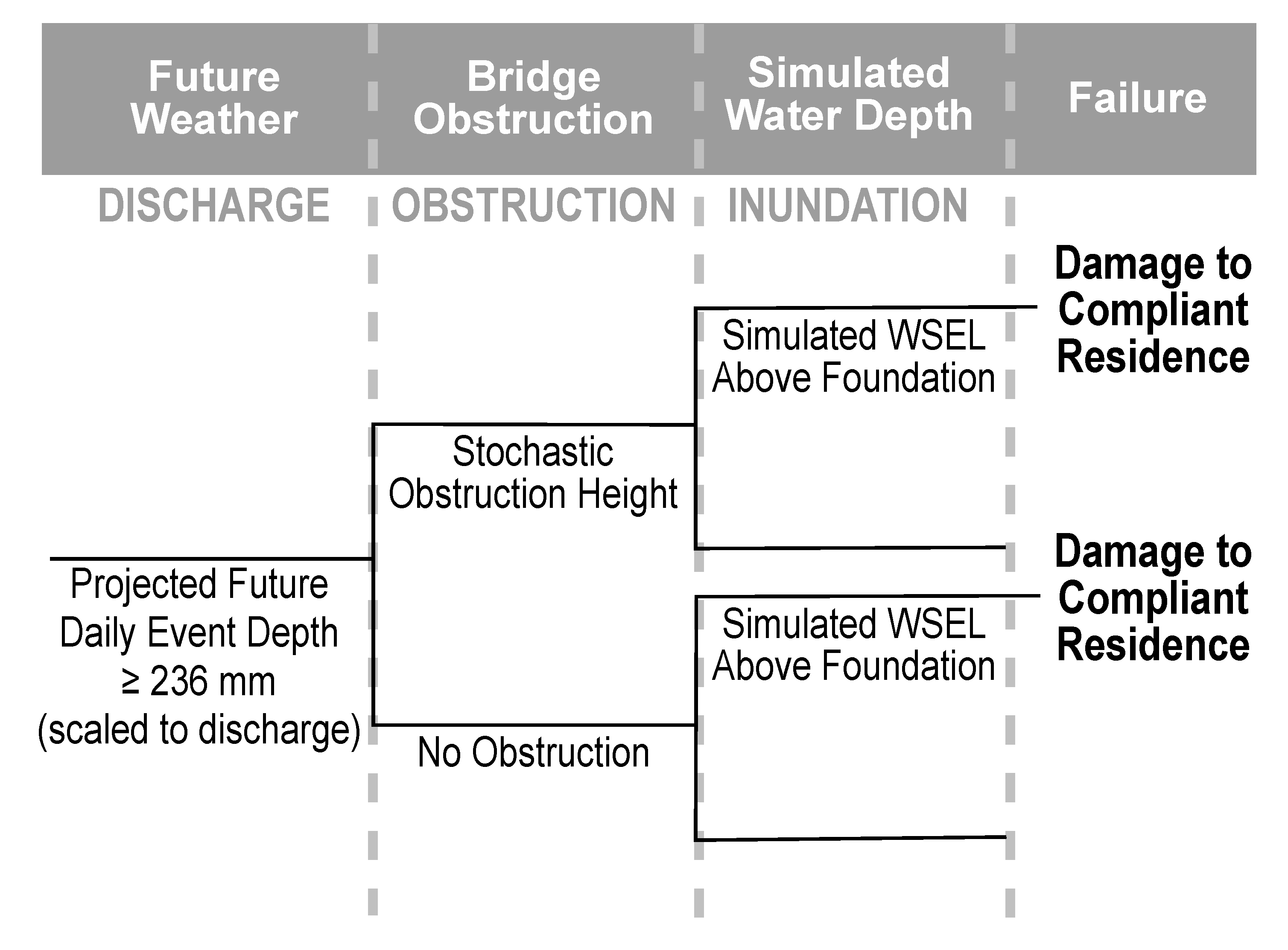
2.1. Probabilistic Risk Assessment (PRA)

The purpose of PRA is risk evaluation for risk management and decision making. Traditionally, it is applied to complex engineered systems and extends reliability engineering assessment. Reliability of an engineered or designed component is the probability that the component will not fail during a specified duration. The “mean time to failure” (MTTF) metric is a generally familiar reliability analysis result. In general, reliability analysis focuses on the design basis of a system and employs engineering uncertainty considerations (see Figure 1).

PRA extends reliability assessment to include planning uncertainty considerations (see Figure 2 and Figure 3). The first comprehensive PRA was related to nuclear reactor safety and extended reliability engineering analysis to generate insight into how relatively frequent and minor accidents could initiate a complex chain of events leading to more severe consequences than some infrequent and major accidents [14]. Subsequently, PRA has been used as a basis for the performance assessment of radioactive waste disposal and has been applied to analyze hazards over hundreds of thousands of years. This extremely long planning and analysis time frame requires explicit depiction of future uncertainty and planning uncertainty.

Risk related to decision making regarding complex engineered systems encompasses scenarios, likelihoods, and consequences. Risk management is the reduction in frequency, or likelihood, of adverse scenarios or accidents. Adverse scenarios are outcomes with negative consequences. Preventing accidents requires an understanding of the complete chain of events that need to occur across multiple parts of a complex system to generate failure. Each sequence of events that can cause failure is a scenario. The risk of a particular scenario is the probability that the system will fail generating negative consequences. Use of risk assessment in decision making requires that uncertainty be addressed and quantified through assignment of likelihoods or probabilities to events and that these likelihoods be conditionally propagated through the scenario to determine probabilities for negative consequences [14].

System failure scenarios begin with an initiating event that represents a change from the desired system state. After initiation, the assessment proceeds by identifying pivotal events that may occur and that will exacerbate or mitigate scenario progression toward a full system failure and negative consequences. The sequence of pivotal events is represented by an event tree where each event represents a node in the progression of failure from the initiating event. At each node, an event occurs or does not occur that propels or mitigates the final consequences of the scenario. An individual event in an event tree can be represented with a fault tree, which provides detailed logical relationships between complex and basic component failures [14]. In PRA, each event in an event tree and each fault in a fault tree is represented probabilistically to describe the likelihood of the event or fault occurring and the uncertainty associated with occurrence in isolation from the system.

Event Tree and Initiating Event

Figure 4 is the event tree for this PRA and provides the flow chart for this study. System failure is flood inundation above the foundation elevation for one or more of the 44 houses in the synthetic site configuration shown in Figure 5. Foundation elevation for each house is provided in Appendix A,

Table A1. Elevations and locations for inundation determination.

House Index	Row	Col	Topo. El. (m)	Foundation El (m)	House Index	Row	Col	Topo. El. (m)	Foundation El. (m)
1	114	27	109.35	109.63	23	114	40	101.85	104.30
2	119	27	109.10	109.38	24	119	40	101.60	104.05
3	124	27	108.85	109.13	25	124	40	101.35	103.80
4	129	27	108.60	108.88	26	129	40	101.10	103.55
5	134	27	108.35	108.63	27	134	40	100.85	103.30
6	139	27	108.10	108.38	28	139	40	100.60	103.05
7	144	27	107.85	108.13	29	144	40	100.35	102.80
8	149	27	107.60	107.88	30	149	40	100.10	102.55
9	154	27	107.35	107.63	31	154	40	99.85	102.30
10	159	27	107.10	107.38	32	159	40	99.60	102.05
11	164	27	106.85	107.13	33	164	40	99.35	101.80
12	114	31	101.85	104.30	34	114	44	109.35	109.63
13	119	31	101.60	104.05	35	119	44	109.10	109.38
14	124	31	101.35	103.80	36	124	44	108.85	109.13
15	129	31	101.10	103.55	37	129	44	108.60	108.88
16	134	31	100.85	103.30	38	134	44	108.35	108.63
17	139	31	100.60	103.05	39	139	44	108.10	108.38
18	144	31	100.35	102.80	40	144	44	107.85	108.13
19	149	31	100.10	102.55	41	149	44	107.60	107.88
20	154	31	99.85	102.30	42	154	44	107.35	107.63
21	159	31	99.60	102.05	43	159	44	107.10	107.38
22	164	31	99.35	101.80	44	164	44	106.85	107.13

. Failure is evaluated by moving along the sequence of events from the initiation of the event until the determination of the amount of inundation.

The initiating event is a daily precipitation depth greater than or equal to 236 mm (9.3 in), which is the 24 h, 25-year recurrence rainfall estimate from Ref. [41] for the Frio River basin calculated in the 2010s. For context, the 24 h, 100-year recurrence rainfall estimate from Ref. [42] for the Frio River basin is 233.7 mm (9.2 in), which was calculated in the 1960s. Hypothetically, the 233.7 mm precipitation depth would have been used as design criteria for the 1% probability annual exceedance flood event if the assets in the synthetic study site configuration (see Figure 5) were constructed between 1965 and 2010. Consequently, we assume that no flooding occurs from daily precipitation depths less than 236 mm. Comparison of the estimates provided by Refs. [41,42] identifies that a rainfall intensity of 236 mm/day is four times more likely to occur under present-day conditions than 30 to 40 years ago.

A collection of 1000 future weather realizations is examined to obtain the collection of initiating events, and Section 2.2 details the generation of these future weather realizations. For each day within a realization, synthetic daily precipitation is compared to 236 mm to determine whether an initiating event occurs. When the initiating event occurs, precipitation depth is scaled to a reach inflow discharge so that flood inundation can be simulated as discussed in Section 2.3.

A proportionality constant was derived to convert 236 mm of daily precipitation to a discharge of 180 m³/s–days. This proportionality constant (180 m³/s–days/ 236 mm = 0.7627 m³/s–days/mm) is conceptually similar to the runoff coefficient, C, in the Rational Method [43], and it was selected because a 180 m³/s–days input discharge, with an obstruction height of 0.0 m, does not generate foundation inundation and system failure for the synthetic site configuration. Note that we are not attempting to derive synthetic land cover conditions for the hypothetical site configuration. In other words, no flood inundation results from 236 mm of daily precipitation depth (with no channel obstruction), which demonstrates that the bridge and houses were designed and built in compliance with the historical requirements of no flooding from the 24 h, 100-year recurrence rainfall estimate of 233.7 m from Ref. [42].

The second event in Figure 4 is obstruction height determination. Both branches from this event are evaluated with the inundation simulation model. The “Stochastic Obstruction Height” branch is the selection of an obstruction height from the probability distribution discussed in Section 2.4, and the “No Obstruction” branch is the specification of an obstruction height of 0.0 m.

“Simulated Water Depth” provides the third and final event in Figure 4. Scaled inflow discharge is evaluated twice as part of this event because both “Bridge Obstruction” branches are simulated using the scaled inflow discharge from the initiating event. The modeling approach presented in Section 2.3 evaluates “Inundation” by comparing the simulated water surface elevation adjacent to each house to its foundation elevation to determine whether there is inundation and flood damage.

When inundation and damage are simulated, there is system failure for one or more regulatory-compliant houses. Estimation of damage costs is discussed in Section 2.5. The total damage cost is summed across all initiating events within each future weather realization. If there are four daily precipitation depth projections greater than or equal to 236 mm in realization number 47, then the total damage for realization number 47 is calculated as the sum of damage estimates from these four initiating events. The result is 2000 (1000 without channel obstruction and 1000 with a randomly sampled channel obstruction) total damage cost estimates from projected climate across 2024–2065 (42 years).

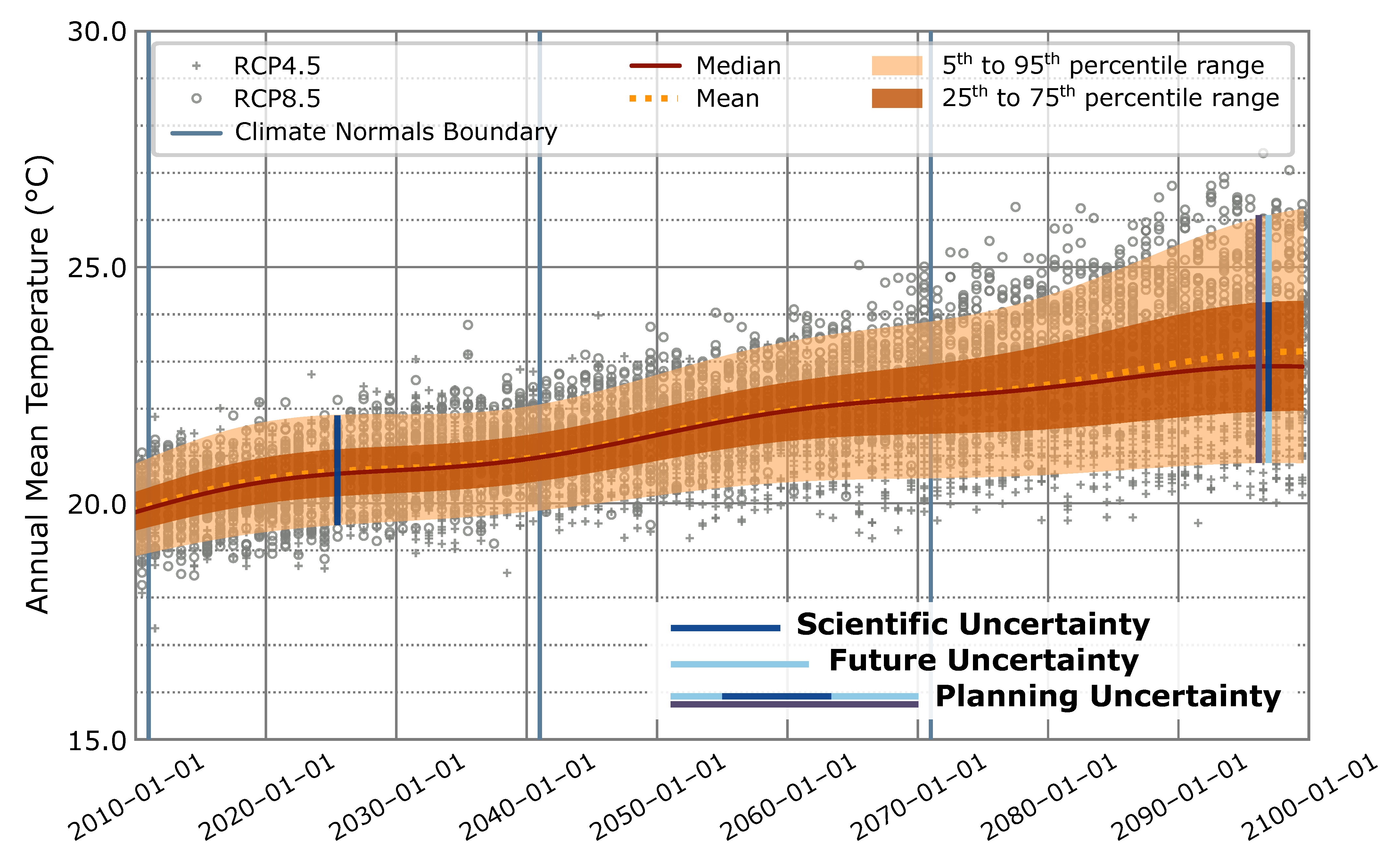
2.2. Future Weather and Climate Inputs

Ref. [40] provides 1000 realizations of synthetic daily weather for 2024–2065 for the Frio Basin that are constrained to reproduce (1) five times more likely severe three-month drought, (2) four times more likely rainfall intensity of 236 mm/day, and (3) annual average precipitation depth observed from 1991 to 2020. The five times more likely severe three-month drought is based on a weather attribution study applicable to the Frio Basin [44]. The four times more likely extreme rainfall intensity comes from the comparison of Refs. [41,42], as discussed in Section 2.1. The expectation of approximately constant annual average precipitation depth comes from analysis of localized constructed analog (LOCA) downscaling of Coupled Model Intercomparison Project, Phase 5 (CMIP5) future climate projections [38]. These 1000 realizations provide the projected future weather used to determine initiating event occurrence.

Synthetic weather series were created using a stochastic weather generator (WG) that was calibrated, or constrained, to produce synthetic series that comply with the constraints on drought, rainfall intensity, and annual average precipitation depth likelihood. To meet both drought and total precipitation depth constraints, discrete events were incorporated into the WG formulation in Ref. [40] to provide for infrequent extreme precipitation events that allowed the calibrated WG to jointly adhere to the competing constraints.

Table 1. Extreme event comparison between NOAA Atlas 14 [41] and the weather generator (WG) with events [40].

Recurrence Interval	24-h Event 1	WG Event Magnitude Range 2
(Year)	(mm)	Lower Bound (mm)	Upper Bound (mm)
2	96	96	153.7
5	141	141	247.6
10	179	179	255.7
25	236	236	290.9
50	285	285	415.5
100	343	343	498.1
200	408	NA 3	NA 3
500	506	NA 3	NA 3
1000	589	NA 3	NA 3

Note(s): ¹ “24 h event depth” comes from Ref. [41]. ² Ref. [40] uses discrete events to represent the extreme events with the recurrence intervals shown. Discrete events are comprised of a Poisson distribution for inter-arrival times, which determine when the event is triggered, and a uniform distribution for event magnitude. “Lower Bound” and “Upper Bound” are the Uniform distribution bounds. WG with discrete events configuration in Ref. [40] provides independent events where more than one event can be triggered for the same wet day. If more than one event is attributed to the same day, the event magnitudes are added to determine the daily precipitation depth. ³ WG with discrete events only uses 2-, 5-, 10-, 25-, 50-, and 100-year events.

lists the discrete event configurations in the WG formulation and compares them with the 24 h precipitation depths provided by Ref. [41]. The 100-year, 24 h event value of 343 mm in Table 1 indicates that the engineering design criteria, related to flooding with a 1% annual probability of exceedance, increased 1.5 times (343 mm/233.7 mm = 1.5) after the bridge and 44 houses were designed and constructed. Note that the discrete event formulation presented in Table 1 provides a possible magnitude of up to 498 mm for the discrete event with an average recurrence interval of 100 years and that the events are independent so that multiple events can occur in the same year and even on the same day. Event independence was required to achieve joint adherence to competing calibration constraints [40].

The initiating event in Figure 4 is daily precipitation depth greater than or equal to 236 mm (9.3 in). Each weather realization is queried for individual days with a simulated precipitation depth that meets the initiating event criterion. When an initiating event is found, flood water surface elevation and foundation inundation depth are determined by simulating the event as discussed in Section 2.3. There are 3583 daily events with a precipitation depth exceeding 236 mm in the 1000 synthetic future weather realizations. Figure 6 shows the distribution of number of initiating events per realization and the likelihood across all realizations per initiating event depth value.

Stationarity

Engineering uncertainty, see Figure 1, is analyzed under the assumption of a fixed and known target. A fixed target requires the assumption of time stationarity, which means that statistical properties and statistical moments of a series are invariant with time. A relaxed form of stationarity, called weak stationarity, is often used for the analysis of water resource observations. It requires a constant mean and an autocovariance function that depends only on the time difference, or lag, and is independent of the points in time that are differenced [45,46]. Weak stationarity only involves the first two statistical moments.

When traditional engineering-style extreme value frequency analysis is implemented, a probability distribution is used to describe event recurrence interval and magnitude [47]. A symmetrical distribution shape, like that provided by the Gaussian or normal distribution, requires the assumption of weak stationarity because unique values for the mean, which is the first statistical moment, and variance, which is the second statistical moment, are required to define the distribution. Nonsymmetrical distribution shapes, like Weibull and Generalized Extreme Value (GEV) distributions, are typically used to represent extremes because it is expected that distribution shape will be skewed towards smaller values. Probability distributions with nonsymmetrical shapes require the assumption of strict stationarity because unique parameter values are required for at least the first three statistical moments to define these distribution forms.

Nonstationarity can be represented when using probability distributions via time-varying parameterization. This is essentially using a custom distribution across an interval. The custom distribution is stationary within its interval but the use of time-varying custom distributions, i.e., among intervals, makes a nonstationary representation overall [48,49]. Refs. [38,39] use piece-wise stationarity, obtained from custom probability distributions for each Climate Normals interval, to represent projected climate across 90 years.

Independent discrete events are employed in the WG as described in Table 1. Each discrete event comprises two probability distributions: (1) a Poisson distribution for inter-arrival time and (2) a uniform distribution for event magnitude. Parameterization of these two distributions is fixed for the WG simulation interval; consequently, each discrete event provides a time stationary depiction of inter-arrival time and magnitude. However, five independent discrete events are used within the WG rather than a single annual event depiction. A time stationary annual event representation would have a fixed distribution for event magnitude that would be sampled each year to produce one important event each year. Five independent discrete events are a significantly different description of precipitation variability when compared to the traditional annual event representation.

Figure 7 shows three data sets that are not stationary relative to each other because each provides a different likelihood for a given weather magnitude. The “SPEI from WG 2031–2060” option in Panel (c) is the synthetic daily weather data set used to determine initiating event occurrence, and Panel (b) “SPEI from LOCA2 2031–2060” version represents global climate, or circulation, model (GCM) projections. Comparison of Panels (b) to (c) indicates that the synthetic daily weather data set, which is used here, shows significantly warmer and drier conditions than the GCM projections. Additionally, Table 1 shows that the synthetic daily weather data also provide an increase in magnitude for extreme precipitation compared to GCM projections because GCM projections in this region tend to underpredict the magnitude of precipitation events compared to NOAA Atlas 14 [38,39].

Note that stationarity is assumed within each data set, shown in Figure 7, as part of the Standardized Precipitation Evapotranspiration Index (SPEI) because this calculation requires definition of a nonsymmetrical probability distribution. Data sufficiency considerations require that the 2N recurrence interval event is the maximum recurrence interval that can be estimated based on N years of assumed time stationary data [47]. Consequently, the “SPEI from WG 2031–2060” and “SPEI from LOCA2 2031–2060” data sets can only estimate to the 1.67% (=$1/\left(2\times 30\right)$) annual probability of exceedance because of combined stationarity and data sufficiency requirements.

Backward-looking engineering uncertainty analyses are especially problematic when applied to evaluate highly variable data sets like weather and climate. History provides a single realization of weather, which is unlikely to include the full range of extremes that could be produced given a known range of atmospheric, oceanic, and near-earth surface and soil conditions from which to deduce a climate description [38,51]. For example, there is currently no accepted proof of the existence of an upper bound on possible rainfall, i.e., a probable maximum precipitation (PMP) value. PMP values are estimated based on limited historical observations and have been exceeded by observations following the PMP calculation [52].

Although the WG-produced synthetic weather series include an assumption of stationarity across 2024–2065, the goal for the WG constraint and calibration is to produce sufficient variability (or variance in values) to compensate for the planning uncertainty inherent in a cone of uncertainty as shown conceptually in Figure 3. This goal is the attempt to include sufficient variability to cover estimated planning uncertainty at the future end of the cone and to hold this amount of variability constant from the present through the end of the cone of uncertainty as shown in Figure 8. Keeping the variance approximately constant for 2024 to 2065 will result in approximately constant percentile values (i.e., flat lines) and constant uncertainty envelope width [38,39], as shown in Figure 8, in contrast to the standard cone of uncertainty representation that has an increasing mean and variance trend over time. As shown in Figure 8, the target weather magnitudes are those projected for the end of the time series, and it provides an time stationary projection of estimated future conditions.

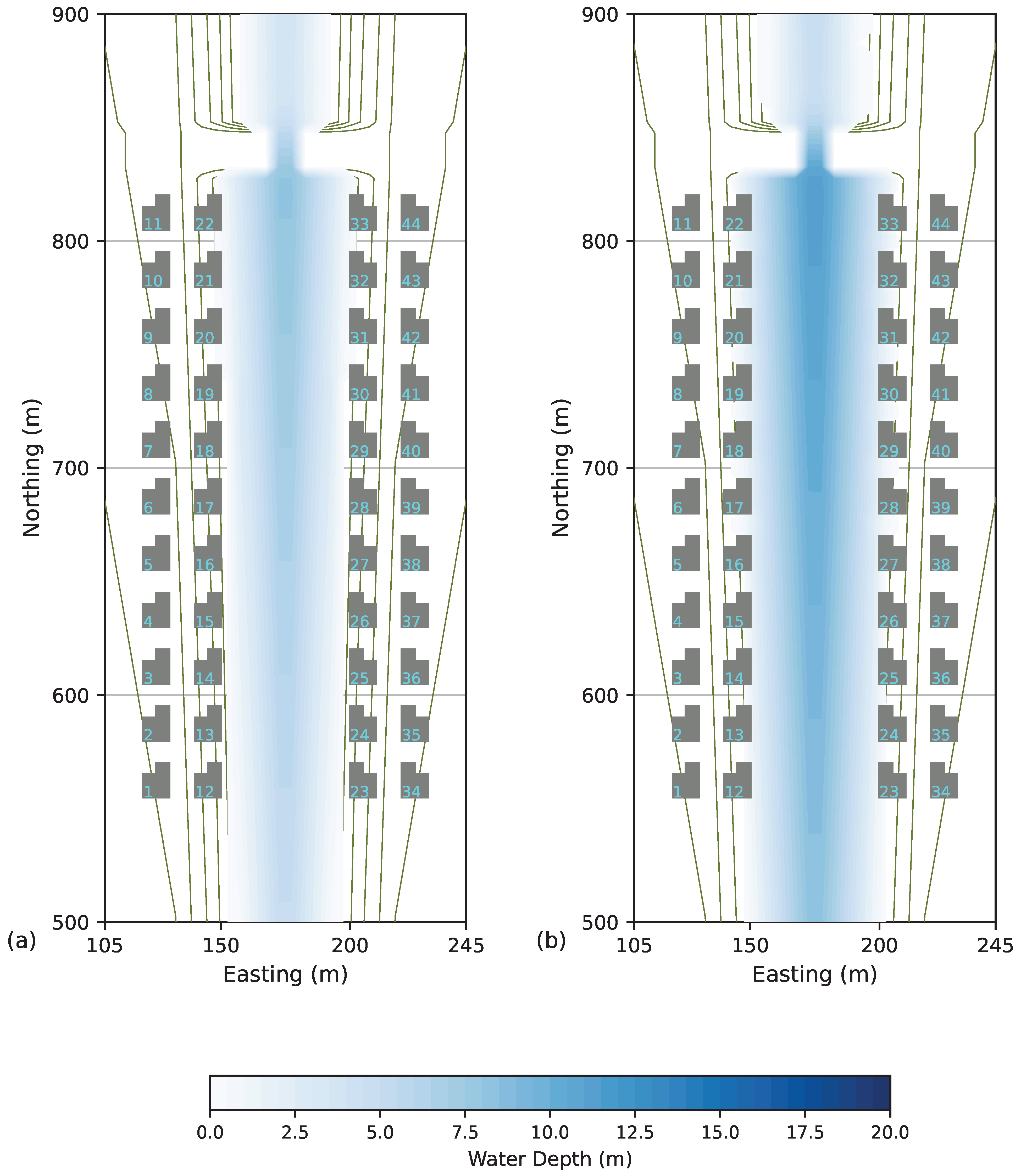
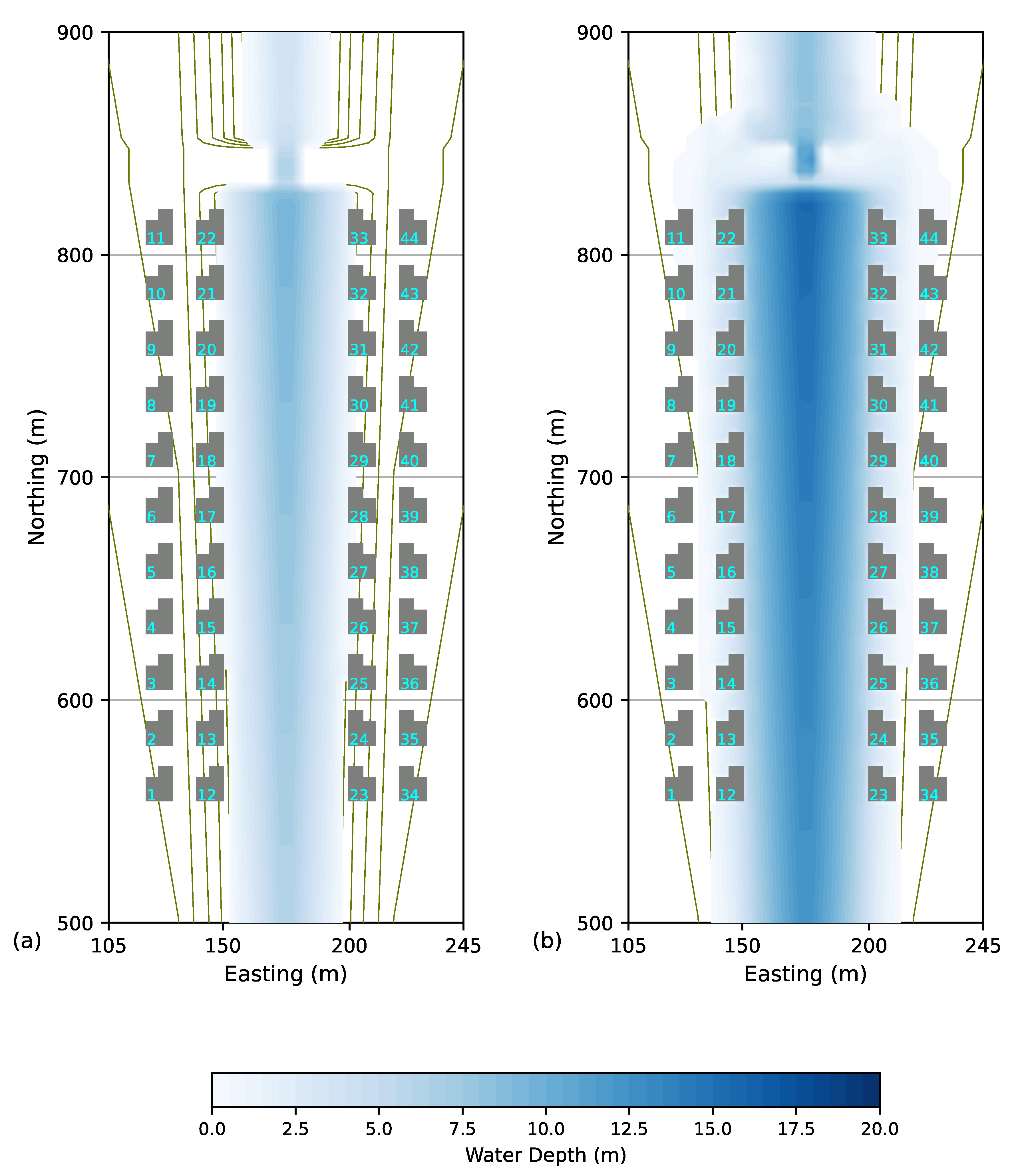
2.3. Inundation Simulation

The study site configuration shown in Figure 5 was designed so that increased inflow discharge could produce a greater degree of flood inundation. The relative channel constriction created by the bridge downstream of the houses ensures that the original design basis event, i.e., an inflow discharge of 180 m³/s corresponding to a daily precipitation depth of 236 mm, passes through the channel constriction without flooding houses. As the inflow discharge increases above 180 m³/s, flood inundation becomes possible because of the conveyance capacity limitation of the bridge opening.

To simulate inundation at the study site, a numerical model must represent (1) a free surface and (2) conservation of momentum. The combined free surface and conservation of momentum representation allows for determination of backwater effects and of increased water depth with partial blockage as momentum is conserved and flow velocity, i.e., kinematic energy, is transformed to water depth, i.e., potential energy, as incompressible water piles up behind the blockage. The MOD_FreeSurf2D model is used to simulate inundation at the study site. It is an open-source and freely available research tool for simulating fluid flow and rivers and streams which provides a combined free surface and conservation of momentum representation [53].

MOD_FreeSurf2D (accessed on 30 January 2025) is the Matlab-based implementation of the semi-implicit, semi-Lagrangian finite-volume approximation to the depth-averaged shallow water equations of Ref. [54] and related work [55,56,57,58]. This is mature, and maybe even legacy, technology from the 1980s and 1990s. The Matlab implementation allows use of well-tested and optimized mathematical libraries, i.e., from Matlab, for combining the mature and elegant numerical methods created and documented by Refs. [54,55,56,57,58]. Ref. [53] summarizes the MOD_FreeSurf2D implementation of these numerical methods and provides dam-break and river flow validation experiments.

A strength of MOD_FreeSurf2D for the study site is the transparent handling of wetting and drying. Channel boundaries within the simulation domain do not require specification, as the model automatically determines wetting or drying in response to any change in flow conditions. It naturally finds the amount of inundation based on topography for small rivers and streams and based on bathymetry for estuaries, reservoirs, and large rivers. The Tidal, Residual, Intertidal Mudflat (TRIM) Model originally presented this efficient solution for wetting and drying, along with the semi-implicit, semi-Lagrangian finite-volume algorithm of Ref. [54]. It was successfully used to simulate tidal currents, tidal driven wetting and drying, and baroclinic forcing for San Francisco Bay in the early 1990s [59].

A fundamental limitation for simulation of flooding considerations with MOD_FreeSurf2D is that it over-estimates fluid velocities in the flood wave because it portrays the depth-averaged shallow water equations and is essentially two-dimensional (2D). A 2D representation over-estimates flood velocity because of the lack of a vertical dimension, which allows vertical velocity to contribute to water piling up behind an obstruction, and a sub-grid turbulence closure, which provides for velocity decay within the water column. This limitation is presented and discussed in the “Application I: Flume experiment dam-break case” of Ref. [53].

MOD_FreeSurf2D Implementation

For the study site, MOD_FreeSurf2D requires specification of (1) volumetric inflow discharge by boundary grid cell, (2) topographic elevations across the domain on a regular grid, (3) initial water depths, which can be zero, across the domain on a regular grid, (4) Manning’s roughness coefficient for each cell in the regular grid, and (5) outflow radiation boundary condition type by boundary grid cell. Each simulation has a duration of six hours and uses a two-second time step. The regular grid is 200 rows by 70 columns of 5 m by 5 m cells.

Inflow discharge is determined by multiplying projected daily precipitation depth by the scaling factor of 180.0 m³/s per 236 mm, as discussed in Section 2.1. Topographic elevations are shown in Figure 5. Cells that are within a house footprint are set to an elevation of 120.0 m so that water has to flow around, and not through, the house for determination of flood water surface elevations. The bridge in Figure 5 is only represented with topographic elevations for ground surface; a bridge deck is not included in the representation. The initial water depths are not critical for obtaining a solution. A “good” initial depth value is anything between zero and a reasonable estimate for the normal water depth for each grid cell location at the onset of flooding. A Manning’s roughness coefficient, or Manning’s N, with a value of 0.040 s/m^1/3 and the radiation free surface outflow boundary condition of Ref. [60] are used for all pertinent cells and simulations.

Figure A1 displays water surface elevations simulated using MOD_FreeSurf2D for the historical design event case in Panel (a) and for the current design event case in Panel (b). The historical design event simulation shows compliance and thus no simulated water elevations above foundation elevations. For the current design event shown in Panel (b), there is simulated flooding of 16 houses with a maximum foundation inundation depth of 2 m for House #33.

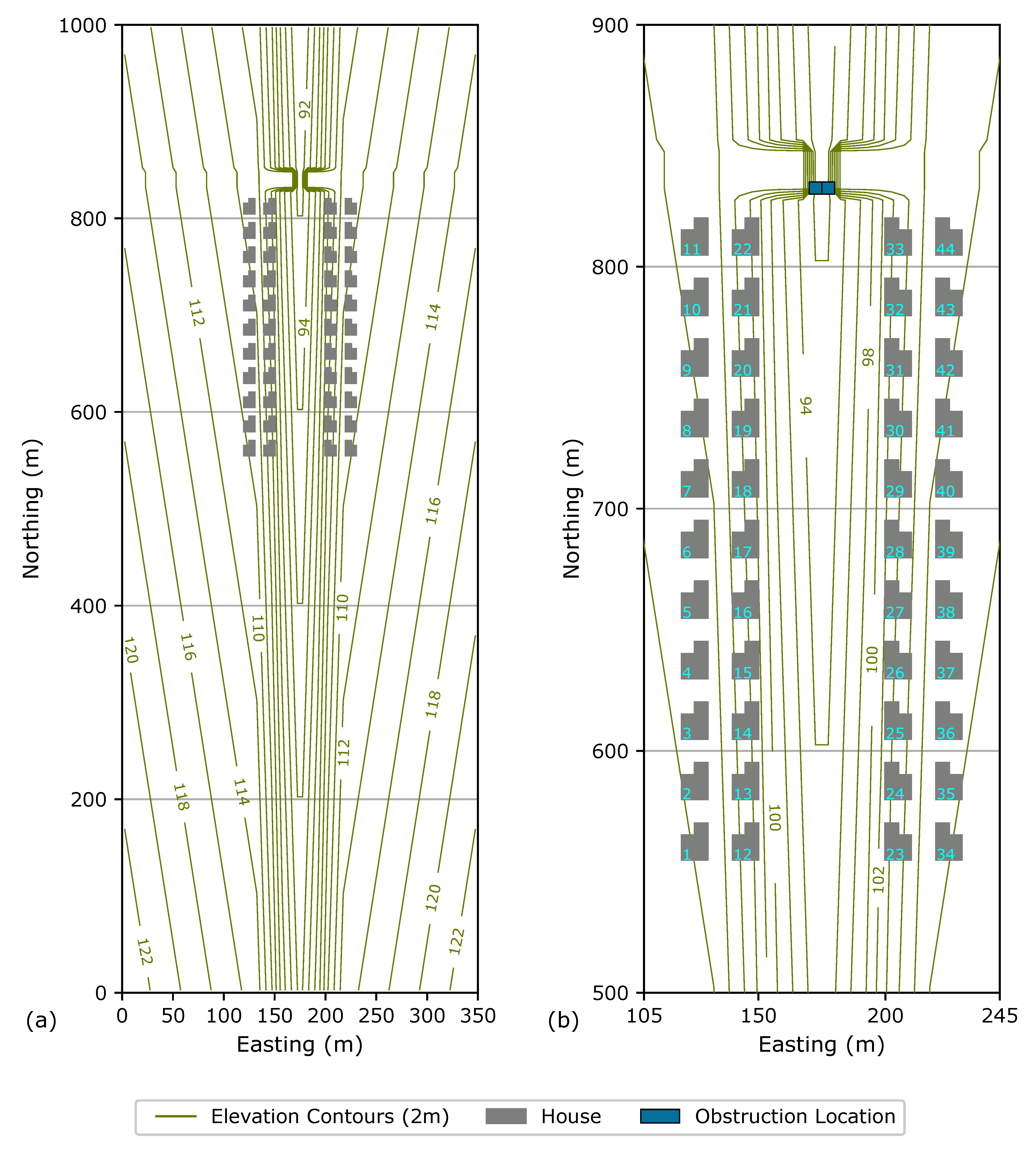
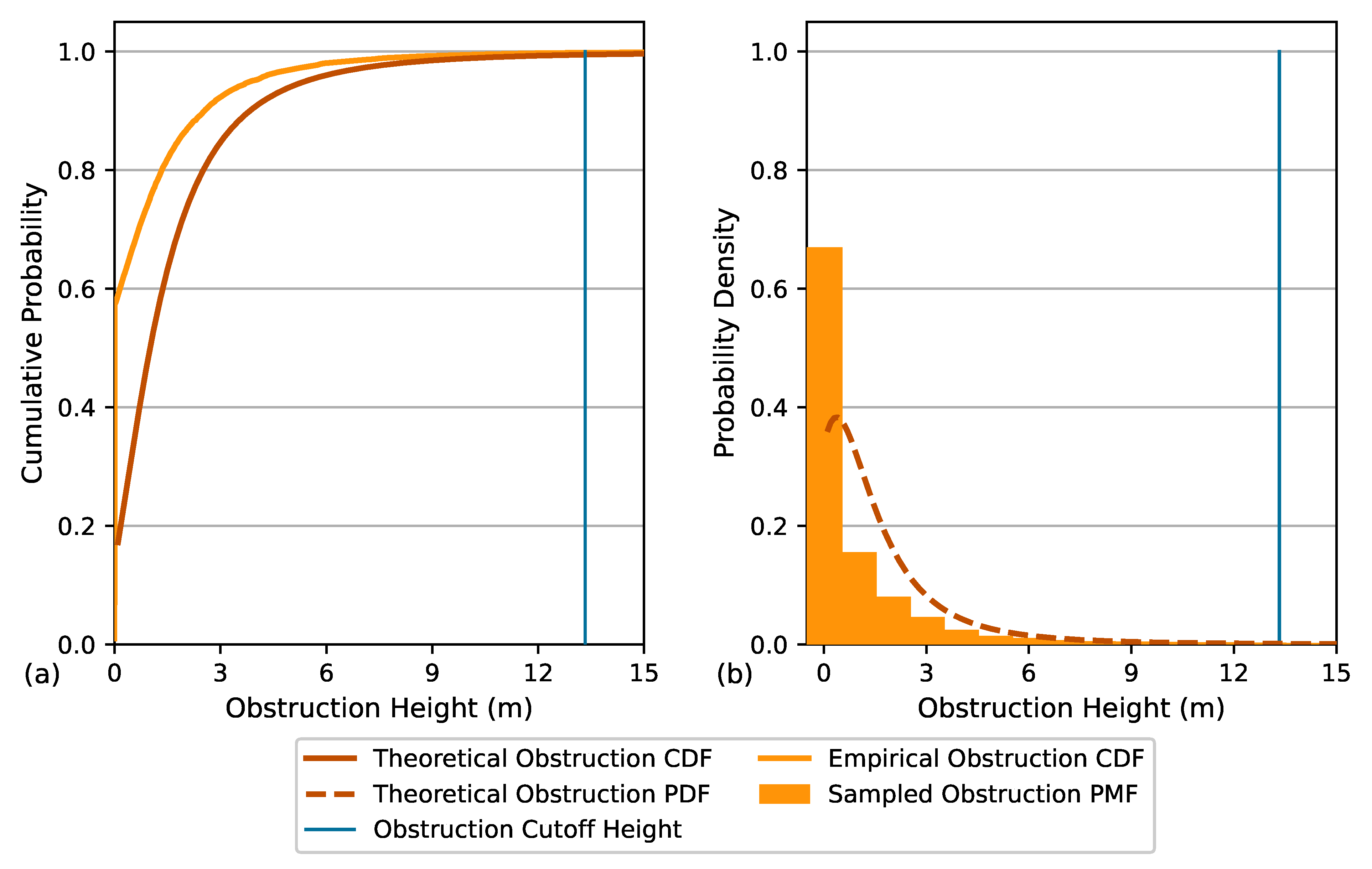
2.4. Obstruction Representation

The “obstruction” event in Figure 4 provides for the inclusion of a stochastic obstruction height as part of the “Stochastic Obstruction Height” branch. All 3583 daily precipitation events are simulated with an obstruction depth of zero on the “No Obstruction” branch and with an obstruction depth randomly sampled from the Generalized Extreme Value (GEV) distribution shown on Figure 9 as part of the “Stochastic Obstruction Height” branch. Consequently, system failure is evaluated 7166 times to determine overall failure likelihood.

“Obstruction height” is a conceptualization of the possible degree of channel blockage by debris transported during the flood event that is caught in the bridge opening. All events simulated in this study exceed the historical 100-year recurrence event magnitude, which was applicable at the time of design. Consequently, it is reasonable to expect the possibility for entrainment of trees, debris, and maybe even structures at these high flood stages and to expect the possibility for debris blockage of the relatively constricted bridge opening. Sampled obstruction height is added to the undisturbed topographic elevation for the two “Obstruction Locations” shown in Figure 5 Panel (b) to increase the topographic elevation seen by the model to undisturbed topographic elevation plus obstruction height. This sum is limited to a maximum elevation value of 105.033 m which is the elevation of the road surface and corresponds to a maximum obstruction height of 13.333 m.

A GEV form was selected for the likelihood of obstruction height because an extreme value-type of representation is desired to produce infrequent or rare large blockage heights. The purpose of PRA is to examine scenarios that are (1) beyond design bases and (2) feasible threats that have not occurred in order to prevent the occurrence and realization of catastrophic negative consequences. As a result, it is accepted practice to select probability distributions to produce the desired likelihood representation. Ref. [29] provides a worked example of high-consequence PRA and illustrates the approach of selecting the type or shape of probability distribution based on whether rare or equally likely events are desired.

The GEV distribution shown on Figure 9 with the “Theoretical Obstruction” lines was created so that obstruction height would be less than or equal to 1.0 m for about 50% of samples. It provides a theoretical formulation because it is defined using closed-form equations for the cumulative distribution function (CDF) and probability density function (PDF). The particular GEV instance shown is obtained by selecting values for three parameters: shape (=−0.3), scale (=1.0), and location (=0.62). For the selected GEV instance, the cumulative probability for an obstruction height of 1 m is 0.498, 0.989 for 10 m, and 0.995 for 13.333 m.

An obstruction height is sampled for the “Stochastic Obstruction Height” branch, and obstruction height is fixed to zero for the “No Obstruction” branch of the event tree. When the distribution of obstruction depths across both branches is examined, the empirical or sampled distribution of obstruction height is normalized to include the half of evaluations that use an obstruction height of zero. The result is the “Empirical Obstruction CDF” shown in Figure 9 Panel (a) and the “Sampled Obstruction PMF” in Figure 9 Panel (b). The probability mass function (PMF) is the normalized histogram of the obstruction heights used across both branches, and a PMF is the discrete and empirical analog to the continuous theoretical PDF.

Figure 10 provides examples of the impact of obstruction height on the simulated elevation of the water surface. Panel (a) shows that an obstruction height of about 5.1 m causes flooding damage for the historical design basis event; however, note that accounting for possible obstruction was not part of the historical design requirements. Panel (b) displays the maximum water surface elevation simulated in the 7166 evaluations. In Figure 10, the application of the obstruction height to the “Obstruction Locations”, shown in Figure 5 Panel (b), is evident from the relatively shallow water depths at these locations.

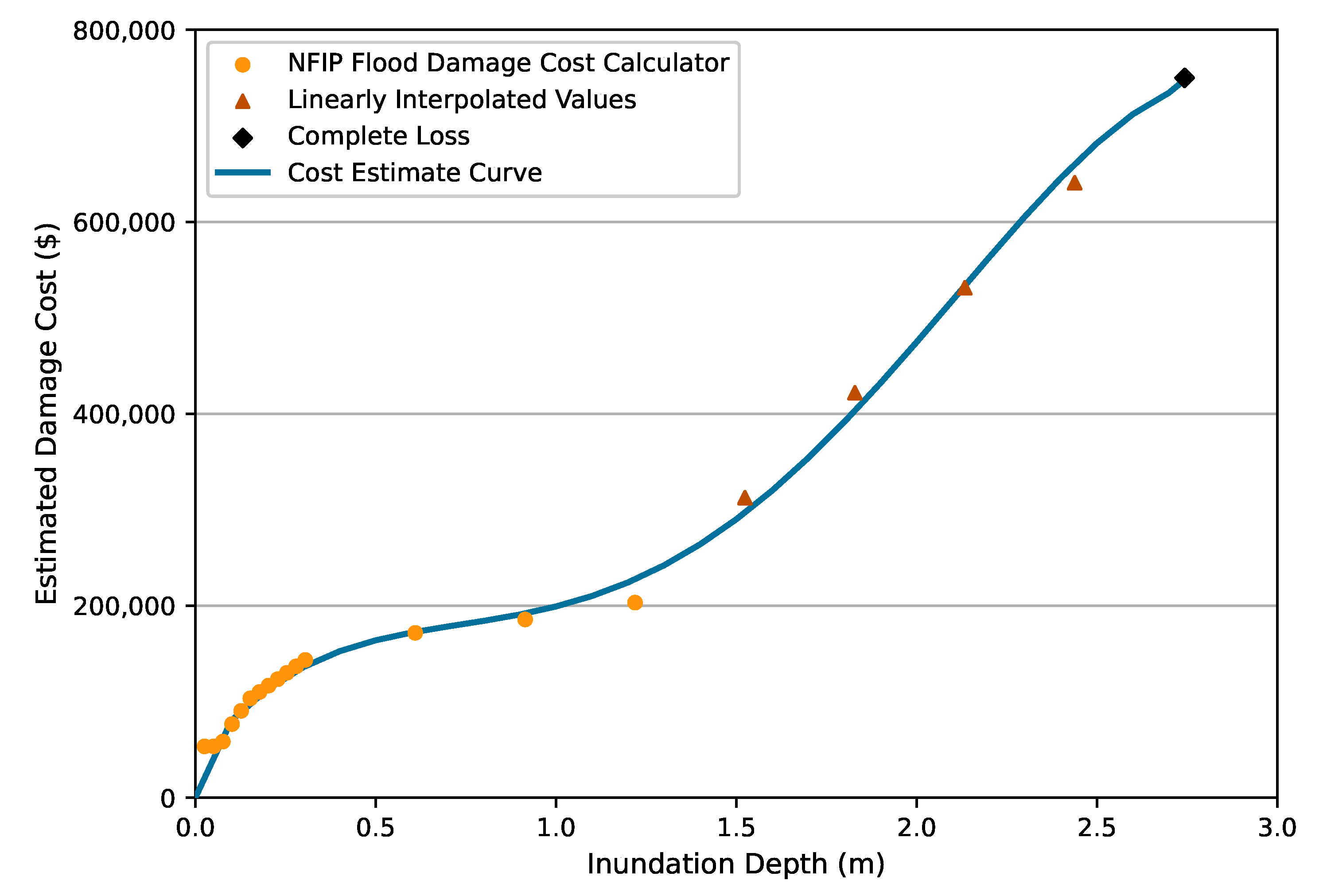
2.5. Damage Cost Estimation

Ref. [61] finds that total building damage is strongly correlated to flood inundation depth above the first finished floor elevation and that flow velocity is important for determining structure component damage. Component damage refers to parts of the building, like internal finishes, that are damaged. Ref. [62] uses simulated inundation depth and the Delft Flood Impact Assessment Tool (Delft-FIAT) [63] to calculate flood damage for the Arch Creek Basin in Florida. Delft-FIAT uses water depth and user-specified depth–damage curves as inputs to evaluate damages per asset where assets include buildings, roads, utilities, etc.

In this study, we use a simple estimate of the damage cost by inundation depth rather than both inundation depth and velocity magnitude to (1) keep the analysis as simple as possible because the study site is synthetic and (2) avoid the velocity estimation limitations of 2D models, discussed in Section 2.3. We develop a single depth–damage curve that applies to all study site houses. The damage curve is applied to estimate cost as part of the PRA without using external tools. Flood inundation assessment is generated using inputs from two precursor events in the event tree: (1) inflow discharge and (2) topographic elevations at the “Obstruction Locations” in Figure 5 Panel (b).

Figure 11 shows the damage cost curve used to attribute the value of damage based on inundation depth. This curve was derived using damage cost estimates by inundation depth from the Federal Emergency Management Administration (FEMA) National Flood Insurance Program (NFIP) online with Flood Damage Cost Calculator (accessed on 3 September 2024) for a 464.5 m² (5000 $f{t}^2$), two-story house. The Flood Damage Cost Calculator provides damage cost estimates for inundation up to 1.219 m (48 in). Damage estimates for inundation depths larger than 1.219 m were determined using linear interpolation between 1.219 m and the assumed “Complete Loss” depth of 2.743 m (108 in). Based on the most recent average real estate values across urban areas and coastal regions across the US, it was assumed that the total value, corresponding to “Complete Loss”, for each house is USD 750,000 [64].

3. Results

System failure is occurrence of a “damage to compliant residence” event in Figure 4. Magnitude of damage is cast to cost using the curve shown in Figure 11. There may be zero to ten initiating events within a weather realization per Figure 6. The total number of initiating events for the ensemble of 1000 weather realizations is 3583, and the damage costs resulting from initiating events within a realization are summed to determine a total cost.

Each future weather realization covers 2024–2065 for this study. The ensemble of future weather realizations provides a probabilistic climate description. Note that each initiating event is evaluated twice due to the “obstruction” event in Figure 4. One evaluation occurs for the “No Obstruction” branch using an obstruction height of 0.0 m, and one occurs for the “Stochastic Obstruction Height” branch using an obstruction height sampled from the theoretical GEV distribution shown in Figure 9. As a result, there are 7166 failure evaluations from 3583 initiating events.

The results and risks are likelihood of total damage or mitigation cost across 2024–2065. Figure 12 displays the CDFs for estimated total cost across the ensemble of 1000 future weather realizations. “All Failures” depict the averaged total cost across both “obstruction” event branches in Figure 4. Total averaged cost for a future weather realization is determined because each initiating event is evaluated twice. “No Obstruction” provides the likelihood of total cost from the obstruction depth fixed to the zero branch, and “Obstruction Only” displays cumulative probability of total cost from the “Stochastic Obstruction Height” branch.

In Figure 12, the largest relative cost increase from inclusion of channel obstruction occurs with likelihood between 60 and 80%. The daily precipitation depth range for 60 and 80% likelihood is approximately 262 to 303 mm from Figure 6 Panel (b). This range provides inflow discharge that can generate minor flooding of two or more houses without factoring in the possibilities for channel obstruction, see Figure A1. When the possibility for channel obstruction is included in the analysis, then any amount of obstruction, combined with inflow discharges in this range, contributes to relatively increased depth of inundation and thus increased damage estimates.

The site geometry, shown in Figure 5, creates an environment where the houses closest to the bridge and to the channel center line are most likely to flood. Figure 13 provides the proportion of initiating events that result in damage to each house. The two houses closest to both the bridge and channel are House #22 and #33, which are damaged in over 35% of event evaluations. Houses #12 and #23 are farthest from the bridge and are only damaged in about 12% of evaluated events.

Table 2. Comparison of likelihoods for cost estimates in millions of USD ¹.

Scenario	Future Mitigation Cost						Current Adaptation Cost 2
	250th Percentile	50th Percentile	Mean	750th Percentile	900th Percentile	Max.
All Failures	0.224	2.461	6.725	11.607	17.099	55.656	NA 3
No Obstruction	0.000	1.272	5.940	10.430	16.193	53.687	NA 3
Obstruction Only	0.325	3.183	7.510	13.590	18.639	57.625	NA 3
Drop 2 Houses	0.025	1.753	5.688	9.818	14.960	48.877	1.5
Drop 4 Houses	0.000	1.104	4.761	8.041	13.054	42.520	3.0
Drop 6 Houses	0.000	0.713	3.944	6.477	11.428	36.705	4.5
Drop 8 Houses	0.000	0.421	3.211	5.030	9.850	31.188	6.0
Drop 10 Houses	0.000	0.173	2.555	3.885	8.251	25.965	7.5
Drop 12 Houses	0.000	0.000	1.964	2.950	6.638	20.972	9.0
Drop 14 Houses	0.000	0.000	1.438	2.038	5.040	16.182	10.5
Drop 16 Houses	0.000	0.000	0.979	1.314	3.504	11.574	12.0
Drop 18 Houses	0.000	0.000	0.588	0.795	2.113	7.251	13.5

Note(s): ¹ “M USD” is million dollars or ×USD 1,000,000. ² “House Removal” is the adaptation approach examined, and it provides the total cost for removing the houses as part of the scenario. Removal cost per house is the total loss cost of USD 750,000. ³ No houses are removed for the “All”, “No Obstruction”, and “Obstruction Only” scenarios; total cost for removing all 44 houses is USD 33 M.

presents likelihood estimates for scenario total cost corresponding to Figure 12 and for the additional adaptation scenarios labeled “Drop 4 Houses”, “Drop 6 Houses”, “Drop 8 Houses”, “Drop 12 Houses”, “Drop 14 Houses”, “Drop 16 Houses”, and “Drop 18 Houses” scenarios. This table shows the same divergence in total estimated mitigation costs across the adaptation scenarios above 60% cumulative probability as shown on Figure 12. The purpose of the “Drop Houses” scenarios is to examine conceptually when it might save money overall to remove houses in the near future, i.e., adaptation, to avoid repeated mitigation costs throughout 2024–2065.

For the “Drop 2 Houses” adaptation scenario examined in Figure 12, Houses #22 and #33 are the two houses dropped from the analysis because these are the two houses most likely to flood. The next two most likely houses to flood are Houses #21 and #32, which are immediately upstream of #22 and #33 in the line of houses closest to the channel on each bank. The “Drop 10 Houses” scenario, shown in Figure 13, is the removal of the five houses closest to the bridge from the line of houses closest to the channel on each bank from damage cost estimations (the houses removed are #22, #21, #20, #19, and #18 from the left bank and #33, #32, #31, #30, and #29 from the right bank). Similarly, the houses dropped from damage cost calculations for the “Drop 18 Houses” scenario are #22, #21, #20, #19, #18, #17, #16, #15 and #14 from the left bank and #33, #32, #31, #30, #29, #28, #27, #26 and #25 from the right bank. These are the 18 houses most likely to be damaged as shown in Figure 13.

Table 3. Likelihood of mitigation cost savings from adaptation via house removal.

Adaptation Scenario	Mitigation Savings Relative to “All Failures” 1 (+Is Savings and −Is Extra Cost, M USD 2)
	25th Percentile	50th Percentile	Mean	75th Percentile	90th Percentile	Max
Drop 2 Houses	—1.301	—0.792	—0.463	0.289	0.639	5.279
Drop 4 Houses	—2.776	—1.643	—1.035	0.566	1.045	10.136
Drop 6 Houses	—4.276	—2.752	—1.718	0.630	1.171	14.451
Drop 8 Houses	—5.776	—3.960	—2.486	0.577	1.248	18.468
Drop 10 Houses	—7.276	—5.213	—3.329	0.222	1.347	22.191
Drop 12 Houses	—8.776	—6.539	—4.239	—0.343	1.461	25.684
Drop 14 Houses	—10.276	—8.039	—5.213	—0.931	1.558	28.974
Drop 16 Houses	—11.776	—9.539	—6.253	—1.707	1.595	32.082
Drop 18 Houses	—13.276	—11.039	—7.363	—2.688	1.485	34.905

Note(s): ¹ Cost savings relative to “All Failures” is calculated from Table 2 as the “All Failures” value less the sum of the “Drop Houses” adaptation scenario mitigation value and the corresponding “House Removal” adaptation cost. ² “M USD” is million dollars or ×USD 1,000,000.

provides estimated cost savings for the likelihoods, or percentiles, shown in Table 2. Cost savings relative to “All Failures” in Table 3 are calculated from Table 2 as the “All Failures” value less the sum of the “Drop Houses” adaptation scenario value and the corresponding “House Removal” adaptation cost. For example, the 90th percentile, the USD 1.0 M cost savings for the “Drop 4 Houses” scenarios, is determined by subtracting the sum of the 90th percentile “Drop 4 Houses” value and “House Removal Cost” for removing four houses from the 90th percentile “All Failures” value ($1.045=17.099-\left(13.054+3.0\right)$).

In Table 3, total cost savings are projected at the 75th percentile level for “Drop 2 Houses”, “Drop 4 Houses”, “Drop 6 Houses”, “Drop 8 Houses”, and “Drop 10 Houses” adaptation scenarios with the maximum cost savings of USD 0.6 M estimated for the “Drop 6 Houses” scenario. All “Drop Houses” scenarios provide estimated cost savings at the 90th percentile and maximum cost (maximum cost is the 100th percentile) levels. Maximum cost savings of USD 1.6 M is estimated for the “Drop 16 Houses” scenario at the 90th percentile level and of USD 34.9 M for the “Drop 18 Houses” scenario at the 100th percentile level.

4. Discussion

This paper presents an approach to optimizing resource use given a current environment of unplanned rapidly changing climate so that future generations can meet their needs safely. Sustainability enters the analysis through decision making based on Table 3 where current generations bear the adaptation costs and future generations pay for the mitigation costs. Specifically, the percentile used for decision making determines the desired degree of sustainability and use of the “Max”, which is the 100th percentile, column in Table 3 provides the most weight towards the ability of future generations to meet their needs. As mentioned previously, the “Drop 18 Houses” adaptation scenario provides the most cost savings for the 100th percentile mitigation costs. In Table 2, the “Max” total cost for the “Drop 18 Houses” adaptation scenario is about USD 7 M, which is approximately equivalent to the “All Failures” mean mitigation cost of USD 7 M. This means that future generations can expect the same degree of damage from the “Drop 18 Houses” adaptation scenario under the worst conditions as from the “All Failures”, or existing conditions, scenario under “expected”, or average, future climate with the adaptation cost of removing 18 houses (USD 13.5 M).

Rapidly changing climate is largely unplanned for because of the backward-looking nature of engineering design bases. Engineering uncertainty relies on the assumption that the “target” value is well known, but not exactly known. It explicitly assumes that everything observed in the future will be similar to what has already been observed in the past. History provides but one realization of weather from which to deduce a climate description. For highly variable quantities, like weather, a single realization is a paltry sample of the daily weather that could be generated from any set of combined atmospheric, biospheric, soil moisture, polar ice pack, and oceanic conditions. Consequently, it is poor decision support to assume that (1) future conditions will never exceed the boundaries provided by recent history and (2) low frequency recurrence intervals, like the 500-year annual event, can be accurately and precisely estimated from historical observations.

In Table 1, the Ref. [41] 100-year recurrence precipitation depth of 343 mm is 1.5 times larger than the historical design basis of 234 mm from Ref. [42]. The constrained WG uniform distribution upper bound estimate is 498 mm, or about 2.1 times larger than the historical basis event, and the lower bound estimate is fixed to 343 mm. Each time the 100-year average recurrence discrete event is triggered in the WG, a daily precipitation depth is sampled from the uniform distribution and thus selected from the range of 343 to 498 mm. Consequently, the synthetic weather series are nonstationary with both current and historical climate. From the empirical CDF in Figure 6b, a precipitation depth of 343 mm has a cumulative probability of 0.866 and a depth of 498 mm has a cumulative probability of 0.991.

The collection of precipitation depths, shown in Figure 6, is an extraction from the 1000 42-year duration daily time series and is not a complete duration annual maximum series. A complete duration annual maximum series provides one maximum value for each year and is required to estimate the recurrence interval in years under the assumption that there is only one major precipitation event (and not multiple similar events or even no events at all) during every year in the series. Even if we wanted to make a traditional (and misguided) estimate of the recurrence interval, the maximum recurrence interval that could be estimated from the probabilistic climate ensemble is the one in 84-year average recurrence event because there are only 42 years in the data set (N = 42 and 2N = 84) [47].

It does not matter which computer model is used to estimate water surface elevation based on inflow discharge and topography in this analysis as long as it meets the basic requirements of a combined free surface and conservation of momentum representation. MOD_FreeSurf2D was used because it was accessible to the authors, it is mature technology, and it runs on a laptop for a simulation domain of the size shown in Figure 5 Panel (a). The style of model needed for this study solves a boundary value problem using a system of partial differential equations (PDEs) across a computational mesh that discretizes the interior of the solution domain.

For boundary value problems, boundary forcing and boundary specification have first-order control over the PDE solution. Parameters like Manning’s N have at best a second-order impact on the PDE solution. The most important component of this analysis is the 1.5-fold increase observed in the primary design basis between 1963 and 2018. This expectation for a large increase in inflow discharge, i.e., boundary forcing, will and does overwhelm all domain interior and numerical model computational parameter considerations. Consequently, parameters like Manning’s N, time integration duration (or time step) and $\Theta$ degree of implicitness are not varied as part of this analysis. Variations in these parameters affect model solutions, but to a much smaller degree than the primary boundary forcing consideration.

Because many of the evaluations use an inflow discharge specification that is 1.5 to 2.1 times larger than the historical design basis event, inflow forcing is expected to be the dominant driver of system failure risk. Obstruction height adjusts channel topography, which is a boundary specification. At the maximum value applied to the model, it creates an approximately 13 m high embankment or dam. Obstruction height also provides a first-order control on likelihood of failure; however, obstruction height is not as significant of a factor as the climate change-driven increase in inflow discharge because it only applies to half of the evaluations. The cumulative probability of the maximum obstruction height of 13.333 m is 0.995, which only applies to the “Sampled Obstruction Height” half of the evaluations. When this cumulative probability is normalized to represent all evaluations, the cumulative probability is 0.9975, which means that an obstruction height of 13.333 m is expected to occur for 0.25% of extreme event evaluations.

4.1. Limitations

We presented a simple and somewhat limited PRA with a single failure scenario. This scenario allows for the evaluation of the risk of flood inundation based on climate change in the existing site configuration, and it provides a template that can be customized for specific sites and real data. However, the event tree or scenario specifically applies to the scenario of backward-looking engineering uncertainty analyses creating a regulatory compliant land use configuration based on historical and largely irrelevant conditions.

The event tree in Figure 4 only treats the scenario of clear water inundation. It is possible that future landslides and debris flows could be important property risks and safety considerations. It is also feasible that erosion and material entrainment under house foundations during extreme events could result in whole house entrainment and movement downstream. Erosion, entrainment, and non-Newtonian flows are not explicitly considered. However, a feasible explanation for the maximum obstruction height of 13.333 m would be whole house entrainment and wedging of the structure in the bridge opening. “Velocity-based” flood damage is not considered because of inherent limitations of 2D models, which conserve momentum, for accurate velocity prediction.

There are also adaptation solutions, beyond simple house removal, that are not examined in this analysis. The relative channel constriction provided by the bridge is the limitation on channel capacity that increases flood inundation risk for nonstationary climate. A direct solution would be to replace the existing bridge with a larger one so that there is no channel constriction. The bridge replacement adaptation solution could be an attractive approach if the existing bridge is beyond its design life and in need of retrofit.

The concept of circularity is related to but different from sustainability [3]. Circularity provides a holistic focus on a complete and closed resource life cycle where there is no terminal event involving disposal and generation of waste. The circular economy is a fairly well-known approach that embodies circularity [65]. Regenerative agriculture and sponge cities are two holistic approaches to natural resources that also embody the concept of circularity. Regenerative agriculture seeks to restore and maintain soil and ecosystem health, address inequity, and leave land, water, and climate in a better shape for the future by focusing on how all aspects of agriculture are connected through a fundamentally regenerative web rather than as linear birth to death supply chain [66]. A sponge city is a nature-based solution where urban areas are designed with abundant natural areas including lakes, parks, wetlands, and stream corridors that provide for storm water management through increased infiltration, natural detention, storage, treatment, and drainage [67,68].

Regenerative agriculture and sponge cities are concepts relevant to this analysis because both seek to increase infiltration, natural detention, and treatment and to reduce fast surface runoff and hazardous flooding. Consequently, regenerative agriculture and sponge city planning could contribute to a holistic planning framework that extends the simple design basis planning and flood safety approach of construct now–pay for damage mitigation throughout the development life span and remove (or worse yet rebuild) facilities as the terminal waste event. PRA is fundamentally limited for holistic analysis because it focuses on failure, risk, and consequent cost. Holistic analysis requires balancing contributions from benefits with cost penalties. Probabilistic cost–benefit analysis is the extension of PRA required to support holistic decision making and to examine planning and design that incorporates circularity.

4.2. Future Work

Examination of PRA utility for sustainable water resource management is implemented at the initial applied research level to minimize implementation costs for exploratory investigation. A synthetic site provided cost savings because an example site was directly created so that many sites did not need to be evaluated to find the exploratory example and because topographic surveys and actual inundation damage curves for each asset did not need to be collected and derived. Table 3 demonstrates that PRA can provide valuable support for sustainable resource management decision making. Given the possibilities for effective decision support, the next phase of work will be a reach–scale demonstration project using a real site with robust site-specific data collection.

An adjustment away from regulatory-based protection and defensive measures based on backward-looking engineering design bases towards holistic planning approaches that reserve floodplains for water conveyance, storage, and non-development beneficial uses and that eliminate development within the entire feasible flood zone [69,70,71] is needed to achieve holistic stewardship rather than parsimonious sustainability. As mentioned previously, PRA provides a tool to promote sustainability considerations in planning; however, it has to be extended to include benefit contributions to fully support circular approaches. A second component of future work will focus on extending PRA to examine and compare non-development-related benefits from and beneficial uses for the feasible flood zone in conjunction with risk analysis for existing flood zone development.

5. Conclusions

An example PRA for flood inundation risk under non-stationary climate is developed and implemented to demonstrate that PRA provides sustainable water resource decision support. Currently, we are experiencing extreme weather events across the globe at different frequencies and with different likelihoods than observed historically. This PRA optimizes current adaptation and potential future mitigation costs given the ongoing issue of existing assets and infrastructure that were designed for climatic conditions that are no longer applicable due to climate change. Weather attribution provides the probabilities and a means to constrain magnitude expectations for future weather and climate so that risk analysis can incorporate future and planning uncertainty.

References

1. Browne, A. Explainer: What Is Sustainability and Why Is It Important? 2022. Available online: https://earth.org/what-is-sustainability/ (accessed on 25 October 2024).
2. United Nations. Sustainability; United Nations: New York, NY, USA, 2024. [Google Scholar]
3. U.S. Chamber of Commerce Foundation. Circularity vs. Sustainability. 2016. Available online: https://www.uschamberfoundation.org/disasters/circularity-vs-sustainability (accessed on 25 October 2024).
4. IPCC. Climate Change 2021: The Physical Science Basis. Contribution of Working Group I to the Sixth Assessment Report of the Intergovernmental Panel on Climate Change; Cambridge University Press: New York, NY, USA, 2021. [Google Scholar] [CrossRef]
5. Otto, F.; Giguere, J.; Clarke, B.; Barnes, C.; Zachariah, M.; Merz, N.; Philip, S.; Kew, S.; Pinto, I.; Vahlberg, M. When Risks Become Reality: Extreme Weather in 2024; World Weather Attribution Annual Report; Imperial College London, Royal Netherlands Meteorological Institute, Red Cross Red Crescent Climate Centre, Imperial College: London, UK, 2024. [Google Scholar]
6. World Weather Attribution (WWA). When Risks Become Reality: Extreme Weather in 2024. 2024. Available online: https://www.worldweatherattribution.org/when-risks-become-reality-extreme-weather-in-2024/ (accessed on 29 January 2025).
7. Vodanube LLC. Uncertainty; Vodanube LLC: Fort Collins, CO, USA, 2024; Available online: https://www.vodanube.com/uncertainty/ (accessed on 28 October 2024).
8. Martin, N.; White, J. Water Resources’ AI–ML Data Uncertainty Risk and Mitigation Using Data Assimilation. Water 2024, 16, 2758. [Google Scholar] [CrossRef]
9. Clarke, B.; Otto, F. Reporting Extreme Weather and Climate Change: A Guide for Journalists; Technical Report; World Weather Attribution (WWA), Imperial College: London, UK, 2023; Available online: https://www.worldweatherattribution.org/wp-content/uploads/ENG_WWA-Reporting-extreme-weather-and-climate-change.pdf (accessed on 3 December 2024).
10. World Weather Attribution (WWA). Exploring the Contribution of Climate Change to Extreme Weather Events. 2024. Available online: https://www.worldweatherattribution.org/ (accessed on 10 October 2024).
11. van Oldenborgh, G.J.; van der Wiel, K.; Kew, S.; Philip, S.; Otto, F.; Vautard, R.; King, A.; Lott, F.; Arrighi, J.; Singh, R.; et al. Pathways and pitfalls in extreme event attribution. Clim. Chang. 2021, 166, 13. [Google Scholar] [CrossRef]
12. Philip, S.; Kew, S.; van Oldenborgh, G.J.; Otto, F.; Vautard, R.; van der Wiel, K.; King, A.; Lott, F.; Arrighi, J.; Singh, R.; et al. A protocol for probabilistic extreme event attribution analyses. Adv. Stat. Climatol. Meteorol. Oceanogr. 2020, 6, 177–203. [Google Scholar] [CrossRef]
13. Hsu, F.; Railsback, J. The Space Shuttle Probabilistic Risk Assessment Framework. In Proceedings of the Probabilistic Safety Assessment and Management, Berlin, Germany, 14–18 June 2004; Spitzer, C., Schmocker, U., Dang, V.N., Eds.; Springer: London, UK, 2004; pp. 1466–1473. [Google Scholar] [CrossRef]
14. Stamatelatos, M.; Dezfuli, H.; Apostolakis, G.; Everline, C.; Guarro, S.; Mathias, D.; Mosleh, A.; Paulos, T.; Riha, D.; Smith, C.; et al. Probabilistic Risk Assessment Procedures Guide for NASA Managers and Practitioners, 2nd ed.; NASA: Hanover, MD, USA, 2011. [Google Scholar]
15. Pan, X.; Ding, S.; Zhang, W.; Liu, T.; Wang, L.; Wang, L. Probabilistic Risk Assessment in Space Launches Using Bayesian Network with Fuzzy Method. Aerospace 2022, 9, 311. [Google Scholar] [CrossRef]
16. Alkhatib, S.; Sakurahara, T.; Reihani, S.; Kee, E.; Ratte, B.; Kaspar, K.; Hunt, S.; Mohaghegh, Z. Phenomenological Nondimensional Parameter Decomposition to Enhance the Use of Simulation Modeling in Fire Probabilistic Risk Assessment of Nuclear Power Plants. J. Nucl. Eng. 2024, 5, 226–245. [Google Scholar] [CrossRef]
17. Lee, J.; Tayfur, H.; Hamza, M.M.; Alzahrani, Y.A.; Diaconeasa, M.A. A Limited-Scope Probabilistic Risk Assessment Study to Risk-Inform the Design of a Fuel Storage System for Spent Pebble-Filled Dry Casks. Eng 2023, 4, 1655–1683. [Google Scholar] [CrossRef]
18. Kubo, K. Accident Sequence Precursor Analysis of an Incident in a Japanese Nuclear Power Plant Based on Dynamic Probabilistic Risk Assessment—Kubo—2023—Science and Technology of Nuclear Installations—Wiley Online Library. Sci. Technol. Nucl. Install. 2023, 2023, 7402217. [Google Scholar] [CrossRef]
19. Han, L.; Fan, Y.; Chen, R.; Zhai, Y.; Liu, Z.; Zhao, Y.; Li, R.; Xia, L. Probabilistic Risk Assessment of Heavy Metals in Mining Soils Based on Fractions: A Case Study in Southern Shaanxi, China. Toxics 2023, 11, 997. [Google Scholar] [CrossRef]
20. Guadalupe, G.A.; Grandez-Yoplac, D.E.; Arellanos, E.; Doménech, E. Probabilistic Risk Assessment of Metals, Acrylamide and Ochratoxin A in Instant Coffee from Brazil, Colombia, Mexico and Peru. Foods 2024, 13, 726. [Google Scholar] [CrossRef]
21. Ololade, I.A.; Alabi, B.A.; Oladoja, N.A.; Ololade, O.O.; Apata, A.O. Occurrence and probabilistic risk assessment of polycyclic aromatic hydrocarbons in blood and urine of auto-mechanics in Akure Metro, Nigeria. Environ. Monit. Assess. 2023, 195, 727. [Google Scholar] [CrossRef]
22. Landquist, H.; Rosén, L.; Lindhe, A.; Hassellöv, I.M. VRAKA—A Probabilistic Risk Assessment Method for Potentially Polluting Shipwrecks. Front. Environ. Sci. 2016, 4, 49. [Google Scholar] [CrossRef]
23. Sawe, S.F.; Shilla, D.A.; Machiwa, J.F. Assessment of Ecological Risk of Heavy Metals Using Probabilistic Risk Assessment Model (AQUARISK) in Surface Sediments from Wami Estuary, Tanzania. Biomed Res. Int. 2021, 2021, 6635903. [Google Scholar] [CrossRef] [PubMed]
24. Shen, H.T.; Pan, X.D.; Han, J.L. Distribution and Probabilistic Risk Assessment of Antibiotics, Illegal Drugs, and Toxic Elements in Gastropods from Southeast China. Foods 2024, 13, 1166. [Google Scholar] [CrossRef] [PubMed]
25. Sheng, D.; Wen, X.; Wu, J.; Wu, M.; Yu, H.; Zhang, C. Comprehensive Probabilistic Health Risk Assessment for Exposure to Arsenic and Cadmium in Groundwater. Environ. Manag. 2021, 67, 779–792. [Google Scholar] [CrossRef]
26. Stehle, S.; Knäbel, A.; Schulz, R. Probabilistic risk assessment of insecticide concentrations in agricultural surface waters: A critical appraisal. Environ. Monit. Assess. 2013, 185, 6295–6310. [Google Scholar] [CrossRef]
27. Zhou, H.; Yue, X.; Chen, Y.; Liu, Y.; Gong, G. Comprehensive Environmental and Health Risk Assessment of Soil Heavy Metal(loid)s Considering Uncertainties: The Case of a Typical Metal Mining Area in Daye City, China. Minerals 2023, 13, 1389. [Google Scholar] [CrossRef]
28. Martin, N.; Nicholaides, K.; Southard, P. Enhanced Water Resources Risk from Collocation of Disposal Wells and Legacy Oil and Gas Exploration and Production Regions in Texas. Jawra J. Am. Water Resour. Assoc. 2022, 58, 1433–1453. [Google Scholar] [CrossRef]
29. Rish, W.R. A probabilistic risk assessment of class I hazardous waste injection wells. In Developments in Water Science, 1st ed.; Underground Injection Science and Technology; Tsang, C.F., Apps, J.A., Eds.; Elsevier Science: Amsterdam, The Netherlands, 2005; Volume 52, pp. 93–135. [Google Scholar] [CrossRef]
30. Bernal, G.A.; Salgado-Galvez, M.A.; Zuloaga, D.; Tristancho, J.; Gonzalez, D.; Cardona, O.D. Integration of Probabilistic and Multi-Hazard Risk Assessment Within Urban Development Planning and Emergency Preparedness and Response: Application to Manizales, Colombia. Int. J. Disaster Risk Sci. 2017, 8, 270–283. [Google Scholar] [CrossRef]
31. Salgado-Gálvez, M.A.; Bernal, G.A.; Zuloaga, D.; Marulanda, M.C.; Cardona, O.D.; Henao, S. Probabilistic Seismic Risk Assessment in Manizales, Colombia: Quantifying Losses for Insurance Purposes. Int. J. Disaster Risk Sci. 2017, 8, 296–307. [Google Scholar] [CrossRef]
32. García-Montiel, E.; Zepeda-Mondragón, F.; Morones-Esquivel, M.M.; Ramírez-Aldaba, H.; López-Serrano, P.M.; Briseño-Reyes, J.; Montiel-Antuna, E. Probabilistic Risk Assessment of Exposure to Fluoride in Drinking Water in Victoria de Durango, Mexico. Sustainability 2023, 15, 14630. [Google Scholar] [CrossRef]
33. Shahsavani, S.; Mohammadpour, A.; Shooshtarian, M.R.; Soleimani, H.; Ghalhari, M.R.; Badeenezhad, A.; Baboli, Z.; Morovati, R.; Javanmardi, P. An ontology-based study on water quality: Probabilistic risk assessment of exposure to fluoride and nitrate in Shiraz drinking water, Iran using fuzzy multi-criteria group decision-making models. Environ. Monit. Assess. 2022, 195, 35. [Google Scholar] [CrossRef] [PubMed]
34. Masoudvaziri, N.; Elhami-Khorasani, N.; Sun, K. Toward Probabilistic Risk Assessment of Wildland–Urban Interface Communities for Wildfires. Fire Technol. 2023, 59, 1379–1403. [Google Scholar] [CrossRef]
35. Monge, J.J.; Dowling, L.J.; Wegner, S.; Melia, N.; Cheon, P.E.S.; Schou, W.; McDonald, G.W.; Journeaux, P.; Wakelin, S.J.; McDonald, N. Probabilistic Risk Assessment of the Economy-Wide Impacts From a Changing Wildfire Climate on a Regional Rural Landscape. Earth’s Future 2023, 11, e2022EF003446. [Google Scholar] [CrossRef]
36. Zhao, H.; Cheng, Y.; Zhang, X.; Yu, S.; Chen, M.; Zhang, C. A Probabilistic Statistical Risk Assessment Method for Soil Erosion Using Remote Sensing Data: A Case Study of the Dali River Basin. Remote Sens. 2024, 16, 3491. [Google Scholar] [CrossRef]
37. Wang, X.; Xia, X.; Zhang, X.; Gu, X.; Zhang, Q. Probabilistic Risk Assessment of Soil Slope Stability Subjected to Water Drawdown by Finite Element Limit Analysis. Appl. Sci. 2022, 12, 10282. [Google Scholar] [CrossRef]
38. Martin, N. Watershed-Scale, Probabilistic Risk Assessment of Water Resources Impacts from Climate Change. Water 2021, 13, 40. [Google Scholar] [CrossRef]
39. Martin, N. Risk Assessment of Future Climate and Land Use/Land Cover Change Impacts on Water Resources. Hydrology 2021, 8, 38. [Google Scholar] [CrossRef]
40. Martin, N. Incorporating Weather Attribution to Future Water Budget Projections. Hydrology 2023, 10, 219. [Google Scholar] [CrossRef]
41. Perica, S.; Pavlovic, S.; St. Laurent, M.; Trypaluk, C.; Unruh, D.; Wilhite, O. NOAA Atlas 14: Precipitation-Frequency Atlas of the United States, Volume 11 Version 2.0: Texas; Technical Report; NOAA: Silver Spring, MD, USA, 2018. [Google Scholar]
42. Hershfield, D.M. Rainfall Frequency Atlas of the United States for Durations from 30 Minutes to 24 Hours and Return Periods from I to 100 Years; Technical Report 40; U.S. Department of Commerce, Weather Bureau: Washington, DC, USA, 1963. [Google Scholar]
43. Chow, V.T.; Maidment, D.R.; Mays, L.W. Applied Hydrology, TATA McGRAW-HILL ed.; McGraw-Hill Education: Gautam Buddha Nagar, India, 1988. [Google Scholar]
44. Schumacher, D.L.; Zachariah, M.; Otto, F.; Barnes, C.; Philip, S.; Kew, S.; Vahlberg, M.; Singh, R.; Heinrich, D.; Arrighi, J.; et al. High Temperatures Exacerbated by Climate Change Made 2022 Northern Hemisphere Soil Moisture Droughts More Likely; Technical Report; World Weather Attribution (WWA), Imperial College: London, UK, 2022. [Google Scholar]
45. Cryer, J.D.; Chan, K.S. Time Series Analysis with Applications in R, 2nd ed.; Springer Texts in Statistics; Springer: New York, NY, USA, 2008. [Google Scholar]
46. Shumway, R.H.; Stoffer, D.S. Time Series Analysis and Its Applications: With R Examples, 4th ed.; Springer: Cham, Switzerland, 2017. [Google Scholar]
47. World Meteorological Organization. Guide to Hydrological Practices, Volume II: Management of Water Resources and Application of Hydrological Practices; World Meteorological Organization (WMO): Geneva, Switzerland, 2009; Volume II. [Google Scholar] [CrossRef]
48. Kyojo, E.A.; Osima, S.E.; Mirau, S.S.; Masanja, V.G. Applying Stationary and Nonstationary Generalized Extreme Value Distributions in Modeling Annual Extreme Temperature Patterns. Adv. Meteorol. 2024, 2024, 9652134. [Google Scholar] [CrossRef]
49. De Paola, F.; Giugni, M.; Pugliese, F.; Annis, A.; Nardi, F. GEV Parameter Estimation and Stationary vs. Non-Stationary Analysis of Extreme Rainfall in African Test Cities. Hydrology 2018, 5, 28. [Google Scholar] [CrossRef]
50. Martin, N. Climate Change and Water Budgets: Accounting for Increased Drought Risk Based on Recent Observations. 2024. Available online: https://sciencefeatured.com/2024/08/21/climate-change-and-water-budgets-accounting-for-increased-drought-risk-based-on-recent-observations/ (accessed on 25 September 2024).
51. Fowler, H.J.; Davies, P.; Lee, S.H. The Climate Is Changing So Fast That We Haven’t Seen How Bad Extreme Weather Could Get. 2024. Available online: http://theconversation.com/the-climate-is-changing-so-fast-that-we-havent-seen-how-bad-extreme-weather-could-get-235726 (accessed on 25 September 2024).
52. National Academies of Sciences, Engineering, and Medicine. Modernizing Probable Maximum Precipitation Estimation; National Academies Press: Washington, DC, USA, 2024. [Google Scholar] [CrossRef]
53. Martin, N.; Gorelick, S.M. MOD_FreeSurf2D: A MATLAB surface fluid flow model for rivers and streams. Comput. Geosci. 2005, 31, 929–946. [Google Scholar] [CrossRef]
54. Casulli, V.; Cheng, R.T. Semi-implicit finite difference methods for three-dimensional shallow water flow. Int. J. Numer. Methods Fluids 1992, 15, 629–648. [Google Scholar] [CrossRef]
55. Casulli, V. Semi-implicit finite difference methods for the two-dimensional shallow water equations. J. Comput. Phys. 1990, 86, 56–74. [Google Scholar] [CrossRef]
56. Casulli, V.; Cattani, E. Stability, accuracy and efficiency of a semi-implicit method for three-dimensional shallow water flow. Comput. Math. Appl. 1994, 27, 99–112. [Google Scholar] [CrossRef]
57. Casulli, V. Numerical simulation of three-dimensional free surface flow in isopycnal co-ordinates. Int. J. Numer. Methods Fluids 1998, 25, 645–658. [Google Scholar] [CrossRef]
58. Casulli, V. A semi-implicit finite difference method for non-hydrostatic, free-surface flows. Int. J. Numer. Methods Fluids 1999, 30, 425–440. [Google Scholar] [CrossRef]
59. Cheng, R.T.; Casulli, V.; Gartner, J.W. Tidal, Residual, Intertidal Mudflat (TRIM) Model and its Applications to San Francisco Bay, California. Estuar. Coast. Shelf Sci. 1993, 36, 235–280. [Google Scholar] [CrossRef]
60. Orlanski, I. A simple boundary condition for unbounded hyperbolic flows. J. Comput. Phys. 1976, 21, 251–269. [Google Scholar] [CrossRef]
61. Paulik, R.; Wild, A.; Zorn, C.; Wotherspoon, L. Residential building flood damage: Insights on processes and implications for risk assessments. J. Flood Risk Manag. 2022, 15, e12832. [Google Scholar] [CrossRef]
62. Peña, F.; Obeysekera, J.; Jane, R.; Nardi, F.; Maran, C.; Cadogan, A.; de Groen, F.; Melesse, A. Investigating compound flooding in a low elevation coastal karst environment using multivariate statistical and 2D hydrodynamic modeling. Weather Clim. Extrem. 2023, 39, 100534. [Google Scholar] [CrossRef]
63. Slager, K.; Burzel, A.; Bos, E.; De Bruikn, K.; Wagenaar, D.; Winsemius, H.; Bouwer, L.; Van der Doef, M. User Guide—Delft FIAT. 2016. Available online: https://deltares.github.io/Delft-FIAT/stable/user_guide/ (accessed on 26 November 2024).
64. National Association of Realtors. Homes for Sale, Apartments & Houses for Rent. 2024. Available online: https://www.realtor.com/ (accessed on 26 November 2024).
65. Ellen Macarthur Foundation. Circular Economy Introduction. 2024. Available online: https://www.ellenmacarthurfoundation.org/topics/circular-economy-introduction/overview (accessed on 25 October 2024).
66. Natural Resources Defense Council (NRDC). Regenerative Agriculture 101. 2021. Available online: https://www.nrdc.org/stories/regenerative-agriculture-101 (accessed on 25 October 2024).
67. Hamidi, A.; Ramavandi, B.; Sorial, G.A. Sponge City—An emerging concept in sustainable water resource management: A scientometric analysis. Resour. Environ. Sustain. 2021, 5, 100028. [Google Scholar] [CrossRef]
68. Harrisberg, K. What Are ’Sponge Cities’ and How Can They Prevent Floods? 2022. Available online: https://climatechampions.unfccc.int/what-are-sponge-cities-and-how-can-they-prevent-floods/ (accessed on 25 October 2024).
69. Mossop, E. Not ‘If’, but ‘When’: City Planners Need to Design for Flooding. These Examples Show the Way. 2021. Available online: http://theconversation.com/not-if-but-when-city-planners-need-to-design-for-flooding-these-examples-show-the-way-157578 (accessed on 18 October 2024).
70. Kelman, I. Disaster by Choice: How Our Actions Turn Natural Hazard…; Oxford University Press: New York, NY, USA, 2020. [Google Scholar]
71. Kelman, I. Floods Are Going to Get Worse: We Need to Start Preparing for Them Now. 2021. Available online: http://theconversation.com/floods-are-going-to-get-worse-we-need-to-start-preparing-for-them-now-172902 (accessed on 18 October 2024).
Figure 1. Engineering uncertainty analysis focuses on accuracy and precision relative to design standards, which provide a defined target. If it is assumed that the target is well known, then uncertainty analysis focuses on accuracy and precision relative to the target. Bias is the inverse of accuracy, and variance is the inverse of precision. Engineering uncertainty is “exact value” uncertainty because the lack of knowledge is high-precision delineation of the bullseye. Reproduced from Ref. [7] (CC-by-4.0).
Water 17 00816 g001
Figure 2. Scientific uncertainty analysis assumes that the true population, or “Truth”, is unknown. Consequently, there is not a well-defined “target” as for engineering uncertainty in Figure 1. A “Biased Truth Estimate”, which is biased sample, is available from indirect observations, and the bias comes from observation error as shown on the figure. When a “Biased Truth Estimate” sample is used to constrain the “Truth” population, extra variability is added, denoted by the extent of the “Extra Variability” circle, to attempt to include the “Truth” population within the area of “good” attempts. The location of the “Truth” sample is unknown and extra variability acts to increase the diameter of the “Extra Variability” circle which means that some “good” attempts may actually be worse than some of the “bad” attempts. Reproduced from Ref. [7] (CC-by-4.0).
Water 17 00816 g002
Figure 3. Planning uncertainty combines the concepts of scientific and future uncertainty. Scientific uncertainty analyses (see Figure 2) attempt to compensate for historical and present-day knowledge limitations and observation error with “Extra Variability”. With enhanced variability of estimates, a range of values with corresponding likelihoods (or probabilities) are used to describe certainty and uncertainty. Future conditions are unknown and will likely include environmental conditions outside of what is expected from historical experience. The farther into the future, the greater the amount of uncertainty. The result is a “cone” of uncertainty for future conditions where the cone spreads as uncertainty increases moving into the future, and the cone provides the value and likelihood combinations that are part of scientific uncertainty analysis. The cone of uncertainty shown on this figure is annual mean temperature cone of uncertainty from Coupled Model Intercomparison Project, Phase 5 (CMIP5), Representative Concentration Pathway (RCP) 4.5, and RCP 8.5 scenarios. Scientific uncertainty is shown conceptually for approximately present-day conditions because it attempts to describe and compensate for historical and present-day knowledge limitations with extra variability. In this figure, there is the same amount of scientific uncertainty in the distant future, i.e., 2095, because it is estimated off of present day and historical conditions and there is no way to estimate it off of unknown future conditions. Future uncertainty is expected to increase moving forward into the future and thus be larger in the distant future. Planning uncertainty is the total of future uncertainty and scientific uncertainty. Reproduced from Ref. [7] (CC-by-4.0).
Water 17 00816 g003
Figure 4. “Precipitation event greater than historical 100-year event” initiating event scenario. This event tree provides the failure scenario evaluated as part of PRA. It is a chain of three events that need to occur for system failure, which is inundation damage to a regulatory-compliant residence. The three events are “discharge”, “obstruction”, and “inundation”. The “discharge” event occurs when daily precipitation amount exceeds the historical design basis precipitation depth of 233.7 mm and the current 24 h, 25-year recurrence interval precipitation depth of 236 mm from Ref. [41]. The “obstruction” event always occurs, and it is an obstruction height of 0.0 m for the “No Obstruction” branch and a stochastically sampled obstruction height for the “Stochastic Obstruction Height” branch. The “inundation” event is always evaluated and involves simulation of the water surface elevations (WSELs) at the site using the input specifications of discharge and obstruction height. System failure is simulated WSEL that exceeds foundation elevation for one or more of the 44 houses, see Figure 5.
Water 17 00816 g004
Figure 5. Synthetic site configuration which provides the study area “map”. Panel (a) displays the entire domain, while Panel (b) shows the focus area including the houses and bridge. The two “Obstruction Locations” shown on Panel (b) are the locations where topographic elevation is increased by the sampled obstruction depth. Inflow discharge is applied at 0 m Northing and typically between 150 and 200 m Easting on Panel (a). Radiation-style outflow boundaries are applied at 1000 m Northing.
Water 17 00816 g005
Figure 6. Precipitation event summary across 1000 future weather realizations covering 2024–2065. Panel (a) identifies the distribution of the number of initiating events that occur within a realization. There is one realization with zero initiating events and one with 10 initiating events. Panel (b) shows cumulative distribution function for all initiating events across the 1000 realizations. The minimum initiating event depth is 236 mm. Maximum projected daily depth is 657 mm.
Water 17 00816 g006
Figure 7. Comparison of the Standardized Precipitation Evapotranspiration Index (SPEI) drought index values for observed 1993–2022, three-month cumulative deficit D values. Panel (a) SPEI based on 1981–2010 observations, Panel (b) SPEI based on Coupled Model Intercomparison Project Phase 6 (CMIP6), Localized Constructed Analogs, Version 2 (LOCA2) projected 2031–2060 conditions, and Panel (c) SPEI based on WG-projected 2031–2060 conditions. SPEI ≤ —1.5 represents severe drought conditions. According to the observed 1981–2010 climate description in Panel (a), severe drought conditions occurred 17 times from 1993 to 2022 with a minimum calculated SPEI of —2.1. Using LOCA2 2031–2060 conditions, severe drought occurred four times between 1993 and 2022, with a minimum SPEI of —1.9. For the 1993–2022 observations analyzed using WG 2031–2060 conditions, no severe droughts occurred, and the minimum SPEI was —1.4. This comparison demonstrates that the WG 2031–2060 climate description is significantly warmer and drier on average than the LOCA2 2031–2060 description. Reproduced from Refs. [40,50] (CC-by-4.0).
Water 17 00816 g007
Figure 8. Schematic example of a 30-year probabilistic description of expected day-to-day weather variability for temperature. The “Weather Generator (WG)—Extra Variability but Stationary”, i.e., blue shading, presents an example of a 30-year probabilistic description of expected day-to-day weather. The “Future—Unobserved and Unknown”, i.e., orange shading and dotted line, portrays the “unknown” and “true” annual average temperature across this 30-year period (2026–2055 in this example). The “Actual” dotted black line represents the series of temperature values that occur. History provides but one realization of weather from which to deduce a climate description. A single realization is unlikely to depict the full range of extremes that could be produced given a known range of atmospheric, oceanic, and near-earth surface and soil conditions [38,51]. The goal for an ensemble of future weather realizations, which is a probabilistic climate description, is to approximately reproduce the total variability in the future cone of uncertainty, i.e., orange shading, at the target end date in the future. The “Weather Generator (WG)–Extra Variability but Stationary” representation is approximately “flat” denoting lack of trend and time stationarity in the representation.
Water 17 00816 g008
Figure 9. Generalized extreme value (GEV) probability distribution used for sampling obstruction height. This GEV instance is defined using shape = —0.3, scale = 1.0, and location = 0.62. Panel (a) displays the Cumulative Density Function (CDF) of the GEV instance. Cumulative probability for 13.333 m is 0.995 and 0.498 for 1.0 m. The “Empirical Obstruction CDF” is also shown; it is the cumulative probability distribution of all obstruction heights used across the 7166 evaluations. Note that half of evaluations (i.e., the “No Obstruction” branch) use an obstruction height of zero, and this is why the “Empirical Obstruction CDF” shows a zero obstruction height for almost 60% of evaluations. Panel (b) shows the Probability Density Function (PDF) for the GEV instance and the “Sampled Obstruction PMF”, which is the normalized histogram of the obstruction heights used across the 7166 evaluations. PMF stands for probability mass function. The “Obstruction Cutoff Height” is 13.333 m and the maximum obstruction height used with the model because it makes the topographic elevation of an “Obstruction Location”, see Figure 5, equal to the elevation of the road.
Water 17 00816 g009
Figure 10. Simulated water depths compared for two simulations using an obstruction height. Panel (a) displays simulated water depth using an inflow discharge of 180.8 m3/s, corresponding to a daily precipitation depth of 237 mm which is similar to the initiating event depth of 236 mm. The sampled obstruction height is 5.1 m. This obstruction height represents the approximate starting point for flooding damage under the historical design conditions. Here, the maximum simulated inundation depth is 0.05 m at House #33, and foundation inundation is simulated for Houses #22 and #33. Total estimated damage cost is USD 105,900. Panel (b) shows the maximum simulated water surface elevation across the 7166 evaluations. Here, water depth is simulated using an inflow discharge of 436.7 m3/s (corresponds to a daily precipitation depth of 572.5 mm) and an obstruction height of 19.9 m (note that obstruction height is truncated to the cutoff height of 13.333 m for implementing the change to topography seen by the model). In this case, the maximum simulated inundation depth is 6.1 m for Houses #22 and #33, and foundation inundation is simulated for Houses #9, #10, #11, #12, #13, #14, #15, #16, #17, #18, #19, #20, #21, #22, #23, #24, #25, #26, #27, #28, #29, #30, #31, #32, #33, #42, #43, and #44. This simulated inundation corresponds to an estimated damage cost of USD 17,273,000 using the approach outlined in Section 2.5.
Water 17 00816 g010
Figure 11. Estimated damage cost curve by inundation depth. The NFIP Flood Damage Cost Calculator (accessed on 3 September 2024) provided damage costs by inundation depth for 0.025 to 1.219 m. It was assumed that an inundation depth of 2.743 m creates a complete loss and that the value of each house is USD 750,000. Cost estimates for inundation depths between 1.219 and 2.743 m were linearly interpolated. Table A2 provides a listing of point values used to interpolate the curve.
Water 17 00816 g011
Figure 12. Cumulative probability for total climate realization damage cost. “All Failures” are the averaged total costs from “Stochastic Obstruction Depth” and “No Obstruction” branches of the Figure 4 event tree. Total averaged cost is determined because each initiating event is evaluated twice, one time for each “obstruction” branch, and it provides normalization for comparison with results from each branch. “No Obstruction” provides the likelihood of total cost from the “No Obstruction” branch, and “Obstruction Only” displays cumulative probability of total cost from the “Stochastic Obstruction Depth” branch. Adaptation measures in this study focus on removal of houses from the reach, and adaptation scenarios are represented with “Drop # Houses” label where # signifies the number of houses removed. “Drop 2 Houses” is the cumulative probability of mitigation cost when Houses #22 and #33, which are closest to the bridge, are removed from the “All Failures” damage cost calculations. “Drop 4 Houses” is the likelihoods for total mitigation cost if houses #21, #22, #32, and #33 are removed.
Water 17 00816 g012
Figure 13. Likelihood for flooding by house. The houses that are closest to both the bridge and the channel center line are most likely to flood given the site layout, see Figure 5. The two closest houses are House #22 and #33, which are damaged in over 35% of the events evaluated. For the “Drop 2 Houses” adaptation scenario examined in Figure 12, Houses #22 and #33 are the two houses dropped from the analysis because these are the two houses most likely to flood. Damage likelihood decreases moving upstream within the lines of houses closest to the channel. For example, Houses #21 and #32 are damaged in over 30% of evaluated events. House #21 is immediately upstream of House #22 on the left bank, and House #32 is immediately upstream of House #33 on the right bank. In the “Drop 4 Houses” adaptation scenario listed in Table 2, Houses #21, #22, #32, and #33 are removed from total cost calculations because these are the four most likely houses to be damaged. For the second line of houses, which is the farthest from the channel center line, Houses #11 and #44 are most likely to flood because they are closest to the bridge. In the maximum water surface elevation simulation, which is shown in Figure 10 Panel (b), only second line Houses #9, #10, #11, #42, #43, and #44 are damaged.
Water 17 00816 g013