
Spatial Distribution, Temporal Behaviour, and Trends of Rainfall Erosivity in Central Italy Using Coarse Data


Abstract
1. Introduction
- A: average annual soil loss (t ha−1);
- R: rainfall erosivity factor (MJ mm ha−1 h−1);
- K: soil erodibility factor (t h ha−1 MJ−1 mm−1);
- L: slope length factor;
- S: slope steepness factor;
- C: cropping and management factor;
- P: erosion control practices factor.
2. Materials and Methods
2.1. Materials
2.2. Methods
2.2.1. Isoerosivity Maps
2.2.2. Model A
2.2.3. Simplified Models for Erosivity Estimation Based on the Event Rainfall Depth he
Model B
Model C
2.2.4. Simplified Model for Erosivity Estimation Based on the Daily Rainfall Depth hd (Model D)
2.2.5. Trend Analyses
3. Results
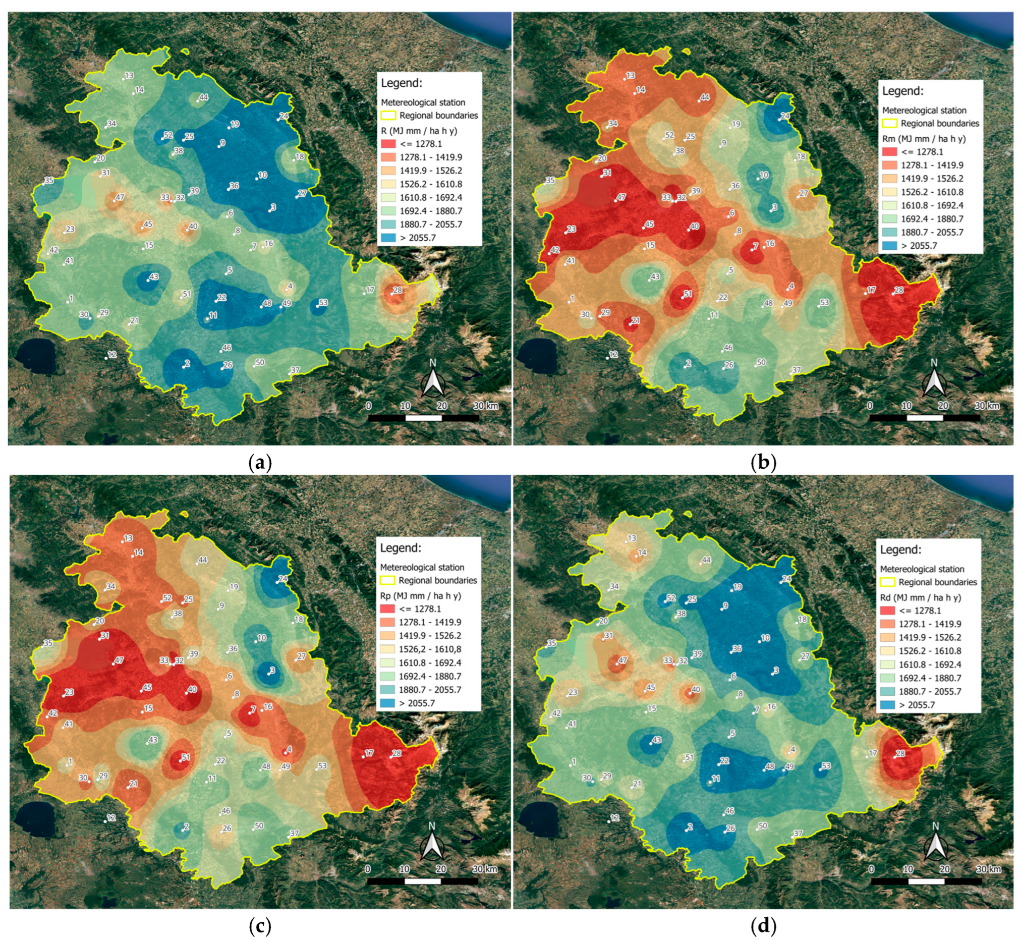
3.1. Model A
3.2. Model B
3.3. Model C
3.4. Model D
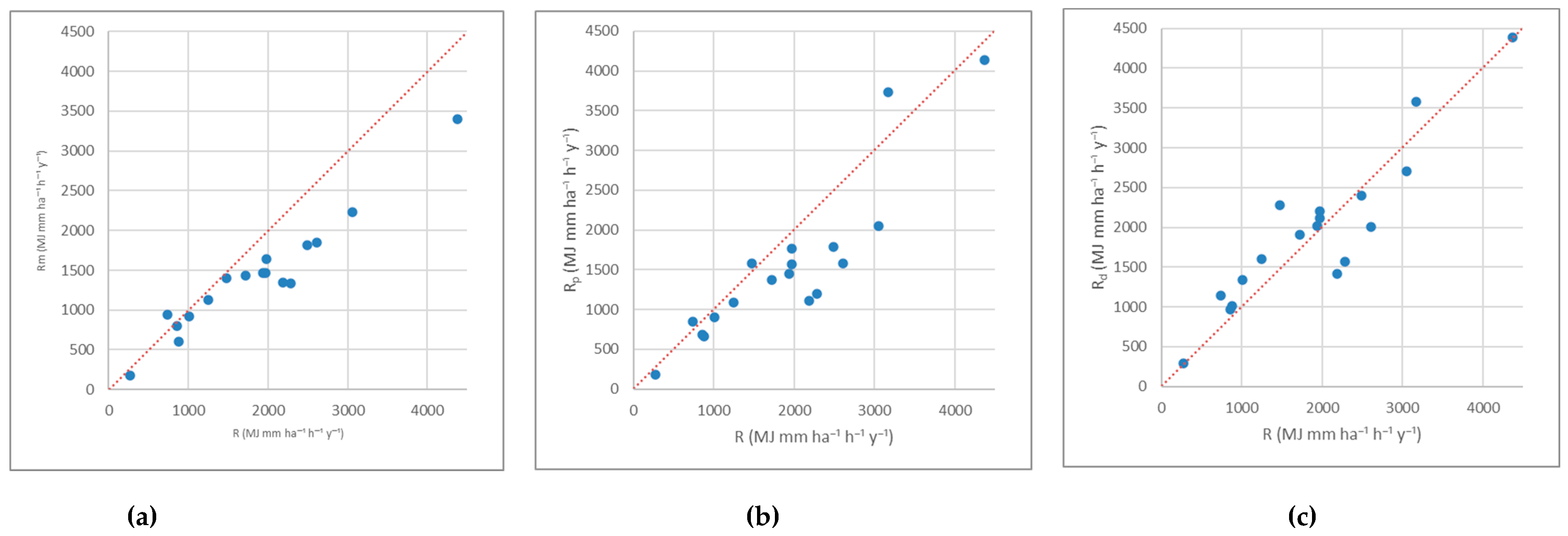
3.5. Model Validation
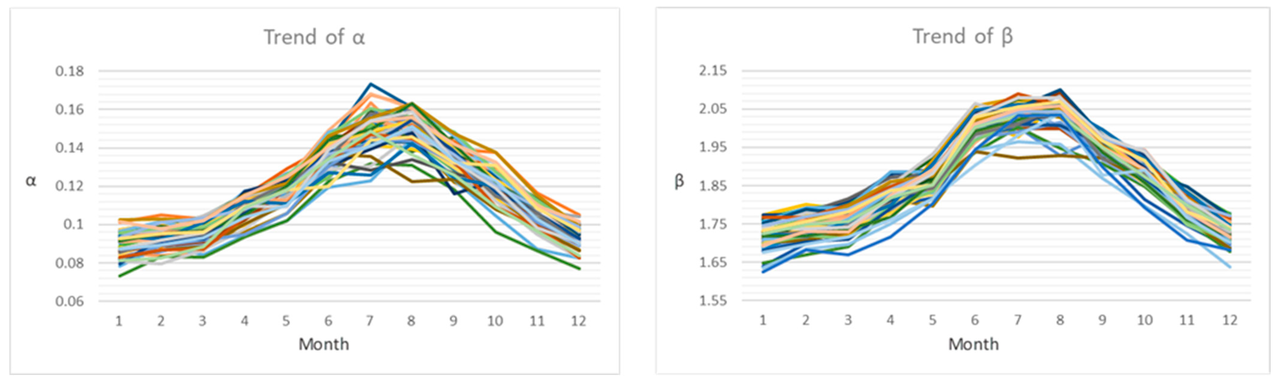
3.6. Trend Analyses
4. Discussion
4.1. Comparison Between Simplified Models (B, C, D) and Reference Model (A)
4.2. Comparison with Panagos et al. (2015) [29]
5. Conclusions
Author Contributions
Funding
Data Availability Statement
Conflicts of Interest
Abbreviations
| USLE | Universal Soil Loss Equation | R | Annual multi-year average erosivity using Model A |
| RUSLE | Revised Universal Soil Loss Equation | Rm | Annual multi-year average erosivity using Model B |
| MAPE | Mean Percent Average Error | Rp | Annual multi-year average erosivity using Model C |
| CV | Coefficient of Variation | Rd | Annual multi-year average erosivity using Model D |
| r | Pearson correlation coefficient | Rw | Winter multi-year average erosivity |
| QGIS | Quantum Geographic Information Science | Rh | Humid multi-year average erosivity |
| IDW | Inverse Distance Weight | Rs | Summer multi-year average erosivity |
| MFI | Modified Fournier Index | P | Annual multi-year average rainfall depth |
| he | Event rainfall depth | Ph | Humid multi-year average rainfall depth |
| Re | Event erosivity | Ps | Summer multi-year average rainfall depth |
| Pw | Winter multi-year average rainfall depth |
Appendix A

| Month | ||||||||||||
|---|---|---|---|---|---|---|---|---|---|---|---|---|
| ID Station | 1 | 2 | 3 | 4 | 5 | 6 | 7 | 8 | 9 | 10 | 11 | 12 |
| 1 | 0.094 | 0.097 | 0.098 | 0.115 | 0.126 | 0.136 | 0.159 | 0.160 | 0.147 | 0.118 | 0.110 | 0.099 |
| 2 | 0.101 | 0.105 | 0.103 | 0.115 | 0.119 | 0.145 | 0.168 | 0.162 | 0.139 | 0.138 | 0.116 | 0.105 |
| 3 | 0.098 | 0.100 | 0.100 | 0.112 | 0.121 | 0.122 | 0.152 | 0.151 | 0.142 | 0.129 | 0.106 | 0.103 |
| 4 | 0.087 | 0.089 | 0.093 | 0.110 | 0.112 | 0.142 | 0.153 | 0.144 | 0.142 | 0.117 | 0.102 | 0.095 |
| 5 | 0.090 | 0.097 | 0.099 | 0.112 | 0.116 | 0.146 | 0.142 | 0.161 | 0.141 | 0.123 | 0.109 | 0.095 |
| 6 | 0.089 | 0.094 | 0.097 | 0.105 | 0.115 | 0.131 | 0.150 | 0.153 | 0.142 | 0.119 | 0.103 | 0.095 |
| 7 | 0.097 | 0.098 | 0.103 | 0.112 | 0.121 | 0.139 | 0.157 | 0.155 | 0.140 | 0.124 | 0.111 | 0.101 |
| 8 | 0.092 | 0.095 | 0.096 | 0.112 | 0.119 | 0.140 | 0.146 | 0.160 | 0.132 | 0.112 | 0.101 | 0.092 |
| 9 | 0.091 | 0.093 | 0.097 | 0.105 | 0.112 | 0.133 | 0.146 | 0.150 | 0.137 | 0.122 | 0.105 | 0.095 |
| 10 | 0.082 | 0.089 | 0.094 | 0.096 | 0.106 | 0.127 | 0.144 | 0.145 | 0.121 | 0.115 | 0.098 | 0.087 |
| 11 | 0.093 | 0.095 | 0.100 | 0.114 | 0.122 | 0.143 | 0.173 | 0.161 | 0.137 | 0.118 | 0.110 | 0.095 |
| 12 | 0.094 | 0.099 | 0.105 | 0.117 | 0.124 | 0.145 | 0.146 | 0.138 | 0.144 | 0.126 | 0.112 | 0.098 |
| 13 | 0.082 | 0.085 | 0.092 | 0.105 | 0.120 | 0.138 | 0.156 | 0.154 | 0.137 | 0.122 | 0.100 | 0.090 |
| 14 | 0.085 | 0.084 | 0.086 | 0.103 | 0.114 | 0.135 | 0.164 | 0.143 | 0.132 | 0.116 | 0.101 | 0.090 |
| 15 | 0.087 | 0.089 | 0.093 | 0.104 | 0.115 | 0.127 | 0.147 | 0.141 | 0.126 | 0.113 | 0.096 | 0.090 |
| 16 | 0.088 | 0.089 | 0.095 | 0.100 | 0.112 | 0.132 | 0.141 | 0.139 | 0.133 | 0.113 | 0.103 | 0.092 |
| 17 | 0.078 | 0.090 | 0.084 | 0.094 | 0.102 | 0.119 | 0.123 | 0.145 | 0.123 | 0.104 | 0.087 | 0.083 |
| 18 | 0.087 | 0.091 | 0.092 | 0.110 | 0.113 | 0.126 | 0.153 | 0.143 | 0.128 | 0.118 | 0.100 | 0.095 |
| 19 | 0.086 | 0.091 | 0.094 | 0.111 | 0.111 | 0.132 | 0.145 | 0.149 | 0.129 | 0.121 | 0.103 | 0.092 |
| 20 | 0.092 | 0.098 | 0.099 | 0.116 | 0.129 | 0.141 | 0.155 | 0.153 | 0.145 | 0.126 | 0.109 | 0.095 |
| 21 | 0.094 | 0.097 | 0.101 | 0.115 | 0.120 | 0.138 | 0.142 | 0.161 | 0.132 | 0.126 | 0.111 | 0.098 |
| 22 | 0.092 | 0.094 | 0.100 | 0.114 | 0.117 | 0.143 | 0.147 | 0.155 | 0.133 | 0.129 | 0.113 | 0.101 |
| 23 | 0.091 | 0.097 | 0.095 | 0.110 | 0.119 | 0.134 | 0.155 | 0.142 | 0.140 | 0.128 | 0.109 | 0.096 |
| 24 | 0.073 | 0.084 | 0.083 | 0.093 | 0.102 | 0.123 | 0.132 | 0.131 | 0.118 | 0.096 | 0.086 | 0.077 |
| 25 | 0.084 | 0.086 | 0.090 | 0.106 | 0.112 | 0.127 | 0.147 | 0.145 | 0.130 | 0.116 | 0.100 | 0.089 |
| 26 | 0.091 | 0.092 | 0.097 | 0.105 | 0.124 | 0.149 | 0.168 | 0.161 | 0.142 | 0.124 | 0.111 | 0.100 |
| 27 | 0.081 | 0.079 | 0.087 | 0.098 | 0.113 | 0.129 | 0.131 | 0.148 | 0.134 | 0.112 | 0.095 | 0.083 |
| 28 | 0.084 | 0.094 | 0.097 | 0.104 | 0.111 | 0.139 | 0.146 | 0.145 | 0.129 | 0.117 | 0.100 | 0.091 |
| 29 | 0.097 | 0.100 | 0.099 | 0.118 | 0.120 | 0.137 | 0.159 | 0.148 | 0.137 | 0.133 | 0.108 | 0.099 |
| 30 | 0.094 | 0.096 | 0.102 | 0.115 | 0.126 | 0.142 | 0.141 | 0.150 | 0.139 | 0.123 | 0.114 | 0.099 |
| 31 | 0.096 | 0.096 | 0.095 | 0.116 | 0.123 | 0.129 | 0.144 | 0.148 | 0.116 | 0.123 | 0.113 | 0.100 |
| 32 | 0.086 | 0.089 | 0.091 | 0.103 | 0.119 | 0.142 | 0.156 | 0.156 | 0.137 | 0.119 | 0.101 | 0.090 |
| 33 | 0.095 | 0.094 | 0.096 | 0.107 | 0.119 | 0.135 | 0.127 | 0.134 | 0.127 | 0.121 | 0.104 | 0.093 |
| 34 | 0.082 | 0.087 | 0.088 | 0.100 | 0.111 | 0.137 | 0.135 | 0.123 | 0.124 | 0.108 | 0.098 | 0.086 |
| 35 | 0.091 | 0.097 | 0.097 | 0.106 | 0.122 | 0.143 | 0.143 | 0.143 | 0.137 | 0.125 | 0.110 | 0.095 |
| 36 | 0.096 | 0.100 | 0.101 | 0.110 | 0.121 | 0.131 | 0.158 | 0.145 | 0.138 | 0.127 | 0.113 | 0.097 |
| 37 | 0.082 | 0.089 | 0.092 | 0.095 | 0.106 | 0.129 | 0.144 | 0.144 | 0.133 | 0.116 | 0.101 | 0.091 |
| 38 | 0.092 | 0.096 | 0.096 | 0.114 | 0.113 | 0.133 | 0.155 | 0.150 | 0.135 | 0.128 | 0.110 | 0.101 |
| 39 | 0.095 | 0.097 | 0.104 | 0.114 | 0.119 | 0.144 | 0.148 | 0.154 | 0.140 | 0.131 | 0.112 | 0.096 |
| 40 | 0.097 | 0.101 | 0.099 | 0.112 | 0.119 | 0.142 | 0.149 | 0.154 | 0.141 | 0.123 | 0.112 | 0.097 |
| 41 | 0.097 | 0.102 | 0.096 | 0.111 | 0.120 | 0.148 | 0.155 | 0.163 | 0.146 | 0.127 | 0.108 | 0.101 |
| 42 | 0.096 | 0.098 | 0.099 | 0.109 | 0.120 | 0.147 | 0.159 | 0.157 | 0.148 | 0.128 | 0.112 | 0.097 |
| 43 | 0.080 | 0.093 | 0.092 | 0.108 | 0.120 | 0.138 | 0.141 | 0.155 | 0.138 | 0.117 | 0.106 | 0.093 |
| 44 | 0.083 | 0.087 | 0.087 | 0.104 | 0.111 | 0.133 | 0.147 | 0.145 | 0.133 | 0.109 | 0.099 | 0.083 |
| 45 | 0.086 | 0.092 | 0.095 | 0.111 | 0.121 | 0.135 | 0.158 | 0.156 | 0.135 | 0.115 | 0.106 | 0.090 |
| 46 | 0.103 | 0.103 | 0.102 | 0.116 | 0.122 | 0.147 | 0.155 | 0.163 | 0.147 | 0.138 | 0.118 | 0.100 |
| 47 | 0.094 | 0.093 | 0.101 | 0.113 | 0.111 | 0.127 | 0.126 | 0.142 | 0.124 | 0.120 | 0.109 | 0.097 |
| 48 | 0.092 | 0.095 | 0.097 | 0.105 | 0.120 | 0.144 | 0.150 | 0.163 | 0.142 | 0.123 | 0.108 | 0.097 |
| 49 | 0.093 | 0.101 | 0.103 | 0.108 | 0.118 | 0.137 | 0.141 | 0.152 | 0.136 | 0.121 | 0.109 | 0.099 |
| 50 | 0.102 | 0.098 | 0.102 | 0.115 | 0.125 | 0.140 | 0.154 | 0.156 | 0.142 | 0.133 | 0.110 | 0.102 |
| 51 | 0.087 | 0.092 | 0.096 | 0.110 | 0.109 | 0.139 | 0.154 | 0.159 | 0.131 | 0.119 | 0.098 | 0.090 |
| 52 | 0.093 | 0.095 | 0.096 | 0.109 | 0.118 | 0.120 | 0.144 | 0.146 | 0.132 | 0.131 | 0.108 | 0.097 |
| 53 | 0.087 | 0.089 | 0.093 | 0.104 | 0.110 | 0.133 | 0.141 | 0.151 | 0.133 | 0.123 | 0.103 | 0.090 |
| 54 | 0.081 | 0.083 | 0.088 | 0.109 | 0.118 | 0.134 | 0.149 | 0.136 | 0.126 | 0.109 | 0.097 | 0.084 |
| Month | ||||||||||||
|---|---|---|---|---|---|---|---|---|---|---|---|---|
| ID Station | 1 | 2 | 3 | 4 | 5 | 6 | 7 | 8 | 9 | 10 | 11 | 12 |
| 1 | 1.694 | 1.719 | 1.727 | 1.805 | 1.887 | 1.975 | 2.048 | 2.057 | 1.981 | 1.858 | 1.792 | 1.713 |
| 2 | 1.717 | 1.736 | 1.727 | 1.843 | 1.859 | 2.014 | 2.072 | 2.051 | 1.968 | 1.936 | 1.820 | 1.730 |
| 3 | 1.779 | 1.801 | 1.786 | 1.798 | 1.815 | 2.028 | 1.978 | 2.066 | 1.922 | 1.874 | 1.804 | 1.781 |
| 4 | 1.733 | 1.762 | 1.793 | 1.842 | 1.898 | 1.993 | 2.017 | 2.058 | 1.942 | 1.928 | 1.804 | 1.777 |
| 5 | 1.764 | 1.790 | 1.804 | 1.857 | 1.859 | 2.007 | 2.037 | 2.058 | 1.980 | 1.924 | 1.840 | 1.777 |
| 6 | 1.757 | 1.757 | 1.794 | 1.865 | 1.872 | 1.994 | 2.027 | 2.040 | 1.981 | 1.909 | 1.815 | 1.756 |
| 7 | 1.696 | 1.728 | 1.740 | 1.819 | 1.838 | 2.003 | 1.999 | 1.999 | 1.922 | 1.865 | 1.766 | 1.708 |
| 8 | 1.762 | 1.780 | 1.817 | 1.875 | 1.881 | 1.988 | 2.019 | 2.042 | 1.997 | 1.915 | 1.829 | 1.759 |
| 9 | 1.689 | 1.724 | 1.724 | 1.814 | 1.797 | 1.943 | 2.047 | 2.025 | 1.933 | 1.863 | 1.767 | 1.699 |
| 10 | 1.761 | 1.770 | 1.797 | 1.829 | 1.858 | 1.991 | 2.038 | 2.055 | 1.975 | 1.905 | 1.828 | 1.763 |
| 11 | 1.758 | 1.766 | 1.800 | 1.851 | 1.920 | 2.032 | 2.075 | 2.062 | 1.957 | 1.910 | 1.833 | 1.757 |
| 12 | 1.679 | 1.711 | 1.739 | 1.812 | 1.860 | 2.002 | 2.004 | 1.929 | 1.965 | 1.900 | 1.809 | 1.715 |
| 13 | 1.707 | 1.764 | 1.758 | 1.835 | 1.874 | 1.982 | 2.016 | 2.066 | 1.979 | 1.867 | 1.778 | 1.741 |
| 14 | 1.734 | 1.756 | 1.765 | 1.827 | 1.888 | 2.020 | 2.037 | 2.085 | 1.934 | 1.914 | 1.788 | 1.740 |
| 15 | 1.744 | 1.772 | 1.795 | 1.846 | 1.879 | 2.015 | 2.066 | 2.061 | 1.971 | 1.919 | 1.816 | 1.754 |
| 16 | 1.757 | 1.792 | 1.792 | 1.885 | 1.886 | 2.008 | 2.008 | 2.048 | 1.982 | 1.914 | 1.826 | 1.770 |
| 17 | 1.734 | 1.763 | 1.755 | 1.823 | 1.863 | 2.025 | 2.048 | 2.037 | 1.917 | 1.869 | 1.800 | 1.752 |
| 18 | 1.640 | 1.698 | 1.716 | 1.797 | 1.826 | 1.983 | 1.991 | 2.059 | 1.923 | 1.810 | 1.747 | 1.690 |
| 19 | 1.693 | 1.724 | 1.716 | 1.792 | 1.836 | 1.999 | 2.034 | 2.041 | 1.968 | 1.896 | 1.757 | 1.706 |
| 20 | 1.701 | 1.722 | 1.765 | 1.806 | 1.856 | 1.993 | 2.009 | 2.008 | 1.953 | 1.872 | 1.775 | 1.724 |
| 21 | 1.732 | 1.735 | 1.721 | 1.783 | 1.915 | 2.057 | 2.078 | 2.055 | 1.980 | 1.883 | 1.786 | 1.716 |
| 22 | 1.686 | 1.724 | 1.754 | 1.840 | 1.895 | 2.013 | 2.043 | 2.005 | 1.932 | 1.877 | 1.778 | 1.703 |
| 23 | 1.651 | 1.671 | 1.692 | 1.782 | 1.849 | 1.937 | 2.010 | 1.948 | 1.916 | 1.858 | 1.758 | 1.679 |
| 24 | 1.699 | 1.736 | 1.737 | 1.798 | 1.838 | 1.966 | 2.054 | 2.005 | 1.918 | 1.855 | 1.764 | 1.694 |
| 25 | 1.720 | 1.746 | 1.765 | 1.841 | 1.836 | 1.962 | 2.046 | 2.039 | 1.950 | 1.943 | 1.809 | 1.756 |
| 26 | 1.741 | 1.779 | 1.787 | 1.850 | 1.932 | 2.064 | 2.036 | 2.068 | 1.990 | 1.895 | 1.844 | 1.768 |
| 27 | 1.714 | 1.746 | 1.737 | 1.813 | 1.826 | 1.986 | 2.051 | 2.061 | 1.937 | 1.855 | 1.766 | 1.728 |
| 28 | 1.635 | 1.681 | 1.697 | 1.753 | 1.806 | 1.941 | 1.964 | 1.961 | 1.862 | 1.791 | 1.721 | 1.639 |
| 29 | 1.702 | 1.721 | 1.738 | 1.819 | 1.837 | 2.032 | 2.052 | 2.035 | 1.978 | 1.872 | 1.751 | 1.701 |
| 30 | 1.701 | 1.737 | 1.730 | 1.836 | 1.851 | 2.041 | 2.044 | 2.054 | 1.974 | 1.897 | 1.772 | 1.716 |
| 31 | 1.712 | 1.718 | 1.728 | 1.779 | 1.850 | 2.032 | 2.038 | 2.094 | 1.965 | 1.891 | 1.758 | 1.702 |
| 32 | 1.718 | 1.742 | 1.755 | 1.812 | 1.882 | 2.007 | 2.023 | 2.034 | 1.950 | 1.880 | 1.776 | 1.747 |
| 33 | 1.702 | 1.710 | 1.729 | 1.782 | 1.849 | 1.942 | 1.916 | 1.928 | 1.923 | 1.864 | 1.762 | 1.687 |
| 34 | 1.752 | 1.789 | 1.775 | 1.814 | 1.872 | 2.019 | 2.054 | 2.100 | 1.978 | 1.887 | 1.848 | 1.769 |
| 35 | 1.712 | 1.746 | 1.754 | 1.832 | 1.867 | 2.012 | 2.030 | 2.052 | 1.962 | 1.863 | 1.823 | 1.726 |
| 36 | 1.704 | 1.722 | 1.753 | 1.788 | 1.839 | 1.972 | 1.994 | 2.021 | 1.934 | 1.868 | 1.768 | 1.701 |
| 37 | 1.719 | 1.763 | 1.771 | 1.842 | 1.851 | 2.011 | 2.038 | 2.043 | 1.972 | 1.888 | 1.822 | 1.740 |
| 38 | 1.690 | 1.743 | 1.743 | 1.791 | 1.840 | 1.980 | 2.024 | 2.054 | 1.958 | 1.866 | 1.774 | 1.730 |
| 39 | 1.701 | 1.743 | 1.740 | 1.780 | 1.839 | 1.978 | 2.031 | 2.045 | 1.968 | 1.875 | 1.785 | 1.704 |
| 40 | 1.709 | 1.719 | 1.763 | 1.833 | 1.830 | 1.992 | 2.038 | 2.063 | 1.952 | 1.865 | 1.777 | 1.702 |
| 41 | 1.697 | 1.722 | 1.712 | 1.797 | 1.835 | 1.969 | 2.015 | 2.063 | 1.970 | 1.855 | 1.755 | 1.704 |
| 42 | 1.681 | 1.703 | 1.711 | 1.791 | 1.859 | 2.009 | 2.011 | 2.022 | 1.958 | 1.870 | 1.785 | 1.682 |
| 43 | 1.767 | 1.766 | 1.799 | 1.849 | 1.885 | 2.033 | 2.089 | 2.060 | 1.977 | 1.916 | 1.820 | 1.765 |
| 44 | 1.720 | 1.730 | 1.746 | 1.821 | 1.843 | 1.983 | 2.011 | 2.060 | 1.921 | 1.883 | 1.784 | 1.718 |
| 45 | 1.730 | 1.756 | 1.798 | 1.861 | 1.874 | 2.022 | 2.043 | 2.053 | 1.955 | 1.889 | 1.817 | 1.744 |
| 46 | 1.723 | 1.718 | 1.756 | 1.797 | 1.907 | 2.038 | 2.063 | 2.060 | 1.997 | 1.919 | 1.835 | 1.747 |
| 47 | 1.715 | 1.724 | 1.738 | 1.766 | 1.858 | 1.993 | 2.009 | 2.060 | 1.941 | 1.858 | 1.760 | 1.718 |
| 48 | 1.745 | 1.770 | 1.788 | 1.839 | 1.887 | 2.005 | 2.043 | 2.042 | 1.971 | 1.937 | 1.804 | 1.771 |
| 49 | 1.695 | 1.731 | 1.729 | 1.825 | 1.892 | 2.011 | 2.049 | 2.055 | 1.949 | 1.892 | 1.781 | 1.720 |
| 50 | 1.739 | 1.736 | 1.741 | 1.819 | 1.883 | 2.033 | 2.080 | 2.079 | 1.979 | 1.940 | 1.813 | 1.741 |
| 51 | 1.731 | 1.756 | 1.781 | 1.837 | 1.853 | 2.029 | 2.055 | 2.070 | 1.958 | 1.915 | 1.781 | 1.740 |
| 52 | 1.676 | 1.697 | 1.715 | 1.761 | 1.817 | 1.902 | 1.982 | 2.037 | 1.877 | 1.889 | 1.768 | 1.700 |
| 53 | 1.724 | 1.747 | 1.756 | 1.818 | 1.853 | 2.004 | 2.032 | 2.035 | 1.949 | 1.874 | 1.798 | 1.735 |
| 54 | 1.626 | 1.682 | 1.670 | 1.717 | 1.803 | 1.944 | 2.033 | 2.035 | 1.899 | 1.792 | 1.708 | 1.683 |
| Period | Period | ||||||
|---|---|---|---|---|---|---|---|
| ID Station | 1 | 2 | 3 | ID Station | 1 | 2 | 3 |
| 1 | 0.098 | 0.116 | 0.148 | 1 | 1.714 | 1.830 | 2.009 |
| 2 | 0.104 | 0.121 | 0.150 | 2 | 1.728 | 1.859 | 2.017 |
| 3 | 0.100 | 0.116 | 0.141 | 3 | 1.785 | 1.821 | 1.996 |
| 4 | 0.092 | 0.110 | 0.144 | 4 | 1.767 | 1.861 | 1.995 |
| 5 | 0.095 | 0.114 | 0.147 | 5 | 1.785 | 1.868 | 2.015 |
| 6 | 0.094 | 0.109 | 0.143 | 6 | 1.777 | 1.873 | 2.016 |
| 7 | 0.100 | 0.117 | 0.146 | 7 | 1.717 | 1.814 | 1.977 |
| 8 | 0.094 | 0.110 | 0.143 | 8 | 1.778 | 1.868 | 2.011 |
| 9 | 0.094 | 0.111 | 0.141 | 9 | 1.715 | 1.806 | 1.980 |
| 10 | 0.088 | 0.103 | 0.132 | 10 | 1.773 | 1.853 | 2.011 |
| 11 | 0.096 | 0.116 | 0.149 | 11 | 1.770 | 1.874 | 2.021 |
| 12 | 0.099 | 0.119 | 0.145 | 12 | 1.710 | 1.838 | 1.985 |
| 13 | 0.087 | 0.111 | 0.144 | 13 | 1.741 | 1.831 | 2.007 |
| 14 | 0.087 | 0.108 | 0.142 | 14 | 1.745 | 1.845 | 2.003 |
| 15 | 0.090 | 0.106 | 0.133 | 15 | 1.764 | 1.862 | 2.025 |
| 16 | 0.092 | 0.107 | 0.135 | 16 | 1.776 | 1.872 | 2.009 |
| 17 | 0.083 | 0.096 | 0.127 | 17 | 1.752 | 1.837 | 1.997 |
| 18 | 0.092 | 0.109 | 0.135 | 18 | 1.688 | 1.789 | 1.981 |
| 19 | 0.091 | 0.111 | 0.137 | 19 | 1.710 | 1.813 | 2.007 |
| 20 | 0.096 | 0.119 | 0.147 | 20 | 1.726 | 1.823 | 1.980 |
| 21 | 0.097 | 0.117 | 0.141 | 21 | 1.726 | 1.832 | 2.035 |
| 22 | 0.097 | 0.118 | 0.142 | 22 | 1.715 | 1.839 | 1.991 |
| 23 | 0.095 | 0.115 | 0.140 | 23 | 1.673 | 1.802 | 1.942 |
| 24 | 0.079 | 0.093 | 0.125 | 24 | 1.718 | 1.810 | 1.971 |
| 25 | 0.087 | 0.108 | 0.135 | 25 | 1.748 | 1.855 | 1.991 |
| 26 | 0.095 | 0.115 | 0.153 | 26 | 1.767 | 1.876 | 2.036 |
| 27 | 0.082 | 0.104 | 0.136 | 27 | 1.731 | 1.808 | 1.996 |
| 28 | 0.091 | 0.108 | 0.139 | 28 | 1.664 | 1.768 | 1.923 |
| 29 | 0.099 | 0.119 | 0.143 | 29 | 1.713 | 1.809 | 2.015 |
| 30 | 0.098 | 0.119 | 0.142 | 30 | 1.720 | 1.830 | 2.021 |
| 31 | 0.097 | 0.119 | 0.131 | 31 | 1.712 | 1.813 | 2.029 |
| 32 | 0.089 | 0.110 | 0.146 | 32 | 1.741 | 1.832 | 1.998 |
| 33 | 0.094 | 0.111 | 0.130 | 33 | 1.704 | 1.809 | 1.927 |
| 34 | 0.086 | 0.104 | 0.130 | 34 | 1.772 | 1.854 | 2.031 |
| 35 | 0.095 | 0.115 | 0.142 | 35 | 1.735 | 1.842 | 2.009 |
| 36 | 0.099 | 0.118 | 0.141 | 36 | 1.720 | 1.815 | 1.972 |
| 37 | 0.088 | 0.104 | 0.136 | 37 | 1.749 | 1.844 | 2.009 |
| 38 | 0.097 | 0.116 | 0.142 | 38 | 1.726 | 1.812 | 2.000 |
| 39 | 0.098 | 0.119 | 0.146 | 39 | 1.721 | 1.817 | 2.003 |
| 40 | 0.099 | 0.117 | 0.145 | 40 | 1.722 | 1.821 | 2.008 |
| 41 | 0.099 | 0.116 | 0.152 | 41 | 1.707 | 1.802 | 1.998 |
| 42 | 0.098 | 0.117 | 0.152 | 42 | 1.698 | 1.819 | 1.993 |
| 43 | 0.090 | 0.112 | 0.142 | 43 | 1.775 | 1.861 | 2.030 |
| 44 | 0.085 | 0.105 | 0.137 | 44 | 1.728 | 1.828 | 1.985 |
| 45 | 0.091 | 0.113 | 0.144 | 45 | 1.758 | 1.855 | 2.013 |
| 46 | 0.101 | 0.121 | 0.152 | 46 | 1.737 | 1.861 | 2.039 |
| 47 | 0.096 | 0.113 | 0.130 | 47 | 1.723 | 1.803 | 2.001 |
| 48 | 0.095 | 0.114 | 0.148 | 48 | 1.768 | 1.861 | 2.011 |
| 49 | 0.099 | 0.114 | 0.140 | 49 | 1.720 | 1.840 | 2.011 |
| 50 | 0.101 | 0.119 | 0.146 | 50 | 1.739 | 1.862 | 2.033 |
| 51 | 0.091 | 0.108 | 0.143 | 51 | 1.753 | 1.841 | 2.020 |
| 52 | 0.096 | 0.116 | 0.135 | 52 | 1.697 | 1.807 | 1.935 |
| 53 | 0.090 | 0.109 | 0.138 | 53 | 1.741 | 1.832 | 1.998 |
| 54 | 0.084 | 0.108 | 0.135 | 54 | 1.668 | 1.752 | 1.964 |
References
- Hewitt, R.; Escobar, F. The Territorial Dynamics of Fast-Growing Regions: Unsustainable Land Use Change and Future Policy Challenges in Madrid, Spain. Appl. Geogr. 2011, 31, 650–667. [Google Scholar] [CrossRef]
- Li, Z.; Fang, H. Impacts of Climate Change on Water Erosion: A Review. Earth-Sci. Rev. 2016, 163, 94–117. [Google Scholar] [CrossRef]
- Dvořák, J.; Novák, L.; Antal, J. (Eds.) Soil Conservation and Silviculture; Developments in Soil Science; Elsevier: Amsterdam, The Netherlands, 1994; ISBN 978-0-08-086991-9. [Google Scholar]
- Uber, M.; Haller, M.; Brendel, C.; Hillebrand, G.; Hoffmann, T. Past, Present and Future Rainfall Erosivity in Central Europe Based on Convection-Permitting Climate Simulations. Hydrol. Earth Syst. Sci. 2024, 28, 87–102. [Google Scholar] [CrossRef]
- Kosmas, C.; Danalatos, N.; Cammeraat, L.H.; Chabart, M.; Diamantopoulos, J.; Farand, R.; Gutierrez, L.; Jacob, A.; Marques, H.; Martinez-Fernandez, J.; et al. The Effect of Land Use on Runoff and Soil Erosion Rates under Mediterranean Conditions. CATENA 1997, 29, 45–59. [Google Scholar] [CrossRef]
- Boardman, J.; Poesen, J. (Eds.) Soil Erosion in Europe, 1st ed.; Wiley: Chichester, UK, 2006; ISBN 978-0-470-85910-0. [Google Scholar]
- Peña-Angulo, D.; Nadal-Romero, E.; González-Hidalgo, J.C.; Albaladejo, J.; Andreu, V.; Bahri, H.; Bernal, S.; Biddoccu, M.; Bienes, R.; Campo, J.; et al. Relationship of Weather Types on the Seasonal and Spatial Variability of Rainfall, Runoff, and Sediment Yield in the Western Mediterranean Basin. Atmosphere 2020, 11, 609. [Google Scholar] [CrossRef]
- Wischmeier, W.H.; Smith, D.D. Predicting Rainfall Erosion Losses: A Guide to Conservation Planning; Agriculture Handbook No. 537; USDA, Science and Education Administration: Washington, DC, USA, 1978.
- Todisco, F.; Vergni, L.; Ortenzi, S.; Di Matteo, L. Soil Loss Estimation Coupling a Modified USLE Model with a Runoff Correction Factor Based on Rainfall and Satellite Soil Moisture Data. Water 2022, 14, 2081. [Google Scholar] [CrossRef]
- Moss, A.; Green, P. Movement of Solids in Air and Water by Raindrop Impact. Effects of Drop-Size and Water-Depth Variations. Soil Res. 1983, 21, 257. [Google Scholar] [CrossRef]
- Bryan, R.B. Soil Erodibility and Processes of Water Erosion on Hillslope. Geomorphology 2000, 32, 385–415. [Google Scholar] [CrossRef]
- Renard, K.G. (Ed.) Predicting Soil Erosion by Water: A Guide to Conservation Planning with the Revised Universal Soil Loss Equation (RUSLE); Agriculture Handbook: Washington, DC, USA, 1997; ISBN 978-0-16-048938-9. [Google Scholar]
- Diodato, N. Estimating RUSLE’s Rainfall Factor in the Part of Italy with a Mediterranean Rainfall Regime. Hydrol. Earth Syst. Sci. 2004, 8, 103–107. [Google Scholar] [CrossRef]
- Capolongo, D.; Diodato, N.; Mannaerts, C.M.; Piccarreta, M.; Strobl, R.O. Analyzing Temporal Changes in Climate Erosivity Using a Simplified Rainfall Erosivity Model in Basilicata (Southern Italy). J. Hydrol. 2008, 356, 119–130. [Google Scholar] [CrossRef]
- Nazzareno, D.; Luigi, G.; Paola, R.; Gerardo, G.; Maria, G.F. Spatial Pattern of Hydrological Predictability of Landslide-Prone Areas. In Engineering Geology for Society and Territory—Volume 2; Lollino, G., Giordan, D., Crosta, G.B., Corominas, J., Azzam, R., Wasowski, J., Sciarra, N., Eds.; Springer International Publishing: Cham, Switzerland, 2015; pp. 1611–1613. ISBN 978-3-319-09056-6. [Google Scholar]
- Bagarello, V.; Ferro, V.; Pampalone, V.; Porto, P.; Todisco, F.; Vergni, L. Predicting Soil Loss in Central and South Italy with a Single USLE-MM Model. J. Soils Sediments 2018, 18, 3365–3377. [Google Scholar] [CrossRef]
- Marques, M.J.; Bienes, R.; Jiménez, L.; Pérez-Rodríguez, R. Effect of Vegetal Cover on Runoff and Soil Erosion under Light Intensity Events. Rainfall Simulation over USLE Plots. Sci. Total Environ. 2007, 378, 161–165. [Google Scholar] [CrossRef]
- Bonilla, C.A.; Vidal, K.L. Rainfall Erosivity in Central Chile. J. Hydrol. 2011, 410, 126–133. [Google Scholar] [CrossRef]
- Di Lena, B.; Curci, G.; Vergni, L. Analysis of Rainfall Erosivity Trends 1980–2018 in a Complex Terrain Region (Abruzzo, Central Italy) from Rain Gauges and Gridded Datasets. Atmosphere 2021, 12, 657. [Google Scholar] [CrossRef]
- Petroselli, A.; Apollonio, C.; De Luca, D.L.; Salvaneschi, P.; Pecci, M.; Marras, T.; Schirone, B. Comparative Evaluation of the Rainfall Erosivity in the Rieti Province, Central Italy, Using Empirical Formulas and a Stochastic Rainfall Generator. Hydrology 2021, 8, 171. [Google Scholar] [CrossRef]
- Mikoš, M.; Jošt, D.; Petkovšek, G. Rainfall and Runoff Erosivity in the Alpine Climate of North Slovenia: A Comparison of Different Estimation Methods. Hydrol. Sci. J. 2006, 51, 115–126. [Google Scholar] [CrossRef]
- Angulo-Martínez, M.; Beguería, S. Estimating Rainfall Erosivity from Daily Precipitation Records: A Comparison among Methods Using Data from the Ebro Basin (NE Spain). J. Hydrol. 2009, 379, 111–121. [Google Scholar] [CrossRef]
- Micić Ponjiger, T.; Lukić, T.; Wilby, R.L.; Marković, S.B.; Valjarević, A.; Dragićević, S.; Gavrilov, M.B.; Ponjiger, I.; Durlević, U.; Milanović, M.M.; et al. Evaluation of Rainfall Erosivity in the Western Balkans by Mapping and Clustering ERA5 Reanalysis Data. Atmosphere 2023, 14, 104. [Google Scholar] [CrossRef]
- Meusburger, K.; Steel, A.; Panagos, P.; Montanarella, L.; Alewell, C. Spatial and Temporal Variability of Rainfall Erosivity Factor for Switzerland. Hydrol. Earth Syst. Sci. 2012, 16, 167–177. [Google Scholar] [CrossRef]
- Vrieling, A.; Hoedjes, J.C.B.; Van Der Velde, M. Towards Large-Scale Monitoring of Soil Erosion in Africa: Accounting for the Dynamics of Rainfall Erosivity. Glob. Planet. Change 2014, 115, 33–43. [Google Scholar] [CrossRef]
- Panagos, P.; Ballabio, C.; Borrelli, P.; Meusburger, K. Spatio-Temporal Analysis of Rainfall Erosivity and Erosivity Density in Greece. CATENA 2016, 137, 161–172. [Google Scholar] [CrossRef]
- Goovaerts, P. Using Elevation to Aid the Geostatistical Mapping of Rainfall Erosivity. CATENA 1999, 34, 227–242. [Google Scholar] [CrossRef]
- Borrelli, P.; Diodato, N.; Panagos, P. Rainfall Erosivity in Italy: A National Scale Spatio-Temporal Assessment. Int. J. Digit. Earth 2016, 9, 835–850. [Google Scholar] [CrossRef]
- Panagos, P.; Ballabio, C.; Borrelli, P.; Meusburger, K.; Klik, A.; Rousseva, S.; Tadić, M.P.; Michaelides, S.; Hrabalíková, M.; Olsen, P.; et al. Rainfall Erosivity in Europe. Sci. Total Environ. 2015, 511, 801–814. [Google Scholar] [CrossRef]
- Todisco, F.; Vergni, L.; Vinci, A.; Pampalone, V. Practical Thresholds to Distinguish Erosive and Rill Rainfall Events. J. Hydrol. 2019, 579, 124173. [Google Scholar] [CrossRef]
- Foster, G.R. RUSLE2 Science Documentation; USDA-Agricultural Research Service: Washington, DC, USA, 2005.
- Brown, L.C.; Foster, G.R. Storm Erosivity Using Idealized Intensity Distributions. Trans. ASAE 1987, 30, 0379–0386. [Google Scholar] [CrossRef]
- Richardson, C.W.; Foster, G.R.; Wright, D.A. Estimation of Erosion Index from Daily Rainfall Amount. Trans. ASAE 1983, 26, 0153–0156. [Google Scholar] [CrossRef]
- Bagarello, V.; D’Asaro, F. Estimating Single Storm Erosion Index. Trans. ASAE 1994, 37, 785–791. [Google Scholar] [CrossRef]
- D’Asaro, F.; D’Agostino, L.; Bagarello, V. Assessing Changes in Rainfall Erosivity in Sicily during the Twentieth Century. Hydrol. Process. 2007, 21, 2862–2871. [Google Scholar] [CrossRef]
- Mann, H.B. Nonparametric Tests Against Trend. Econometrica 1945, 13, 245. [Google Scholar] [CrossRef]
- Kendall, M.G. Rank Correlation Measures; Charles Griffin: London, UK, 1975. [Google Scholar]
- Sen, P.K. Estimates of the Regression Coefficient Based on Kendall’s Tau. J. Am. Stat. Assoc. 1968, 63, 1379–1389. [Google Scholar] [CrossRef]
- Bronaugh, D.; Schoeneberg, A. Zyp: Zhang + Yue-Pilon Trends Package; R Package Version 0.11-1, 2012. Available online: https://CRAN.R-project.org/package=zyp (accessed on 9 March 2025).
- McLeod, A.I. McLeod Kendall: Kendall Rank Correlation and Mann-Kendall Trend Test; R Package Version 2.2.1, 2005. Available online: https://CRAN.R-project.org/package=Kendall (accessed on 9 March 2025).
- Todisco, F.; Brocca, L.; Termite, L.F.; Wagner, W. Use of Satellite and Modeled Soil Moisture Data for Predicting Event Soil Loss at Plot Scale. Hydrol. Earth Syst. Sci. 2015, 19, 3845–3856. [Google Scholar] [CrossRef]
- Todisco, F.; Vergni, L.; Bomba, C. Definizione di modelli semplificati per la stima dell’indice di erosività della pioggia e curve di isoerosività per la regione Umbria. Quad. Idronomia Mont. 2010, 29, 331–347. [Google Scholar]
- Nearing, M.A.; Yin, S.; Borrelli, P.; Polyakov, V.O. Rainfall Erosivity: An Historical Review. CATENA 2017, 157, 357–362. [Google Scholar] [CrossRef]
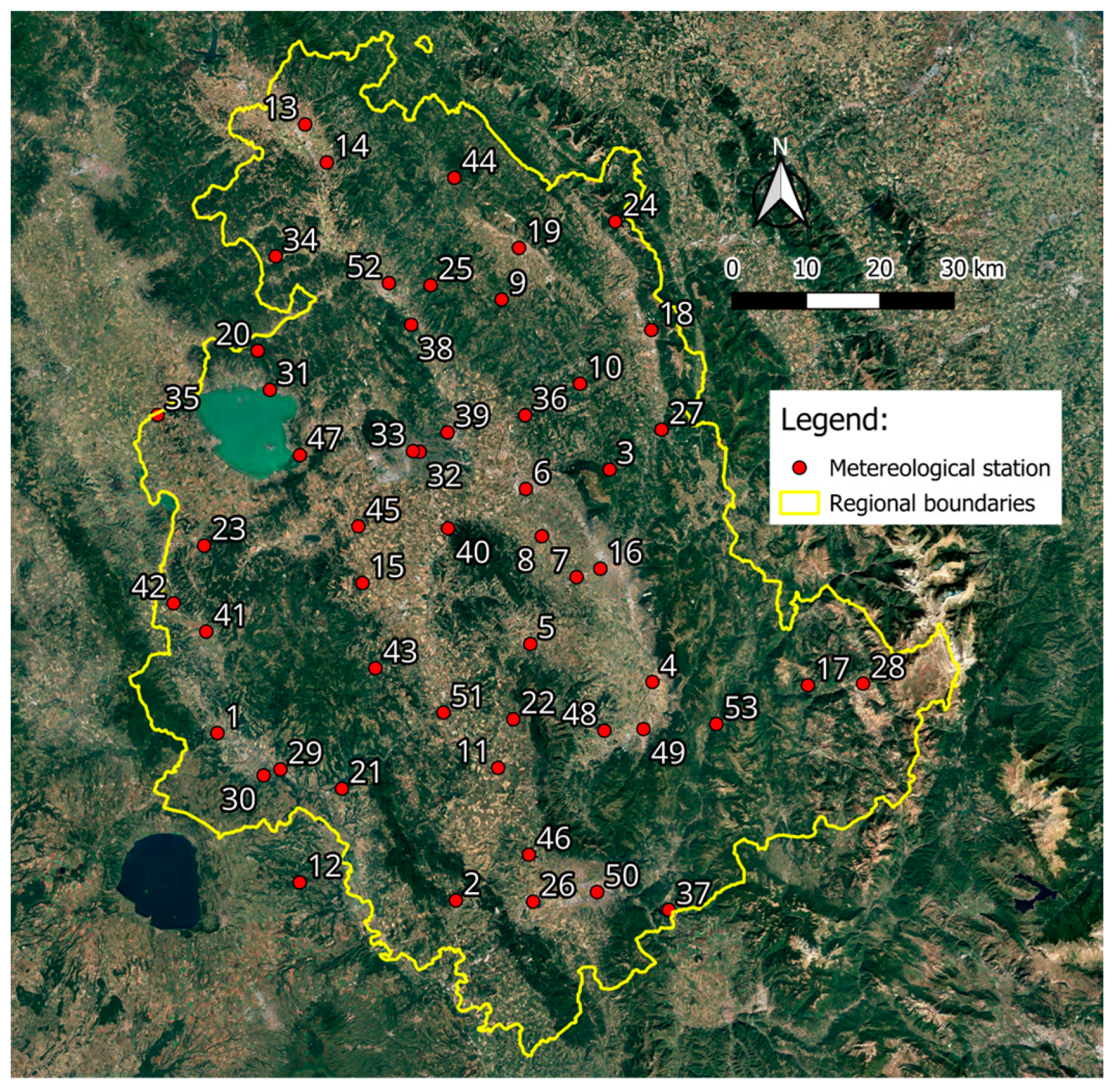


| ID | Metereological Station | Elevation (m a.s.l.) | ID | Metereological Station | Elevation (m a.s.l.) |
|---|---|---|---|---|---|
| 1 | Allerona | 153.2 | 28 | Norcia | 691.3 |
| 2 | Amelia | 319.5 | 29 | Orvieto | 311.4 |
| 3 | Armenzano | 707.7 | 30 | Orvieto Scalo | 109.3 |
| 4 | Azzano | 235.2 | 31 | Passignano sul Trasimeno | 327.8 |
| 5 | Bastardo | 331.5 | 32 | Perugia Fontivegge | 308.5 |
| 6 | Bastia Umbra | 203.3 | 33 | Perugia Santa Giuliana | 433.8 |
| 7 | Bevagna | 211.5 | 34 | Petrelle | 341.9 |
| 8 | Cannara | 191.4 | 35 | Petrignano del Lago | 303.9 |
| 9 | Carestello | 517.8 | 36 | Pianello | 231.5 |
| 10 | Casacastalda | 730.1 | 37 | Piediluco | 370.0 |
| 11 | Casigliano | 272.5 | 38 | Pierantonio | 239.0 |
| 12 | Castel Cellesi | 362.8 | 39 | Ponte Felcino | 191.6 |
| 13 | Cerbara | 310.0 | 40 | Ponte Nuovo Torgiano | 170.0 |
| 14 | Città di Castello | 304.0 | 41 | Ponte Santa Maria | 240.1 |
| 15 | Compignano | 240.2 | 42 | Ponticelli | 244.9 |
| 16 | Foligno | 220.0 | 43 | Ripalvella | 453.1 |
| 17 | Forsivo | 963.2 | 44 | San Benedetto Vecchio | 729.4 |
| 18 | Gualdo Tadino | 596.5 | 45 | San Biagio della Valle | 257.0 |
| 19 | Gubbio | 471.5 | 46 | San Gemini | 297.1 |
| 20 | La Cima | 790.8 | 47 | San Savino | 260.0 |
| 21 | Lago Corbara | 128.0 | 48 | San Silvestro | 379.9 |
| 22 | Massa Martana | 327.9 | 49 | Spoleto | 353.2 |
| 23 | Moiano | 270.3 | 50 | Terni | 123.0 |
| 24 | Monte Cucco | 1087.2 | 51 | Todi | 326.1 |
| 25 | Montelovesco | 634.1 | 52 | Umbertide | 305.7 |
| 26 | Narni Scalo | 108.9 | 53 | Vallo di Nera | 306.7 |
| 27 | Nocera Umbra | 535.7 | 54 | Verghereto | 1069.2 |
| 1 | 2 | 3 | 4 | 5 | 6 | 7 | 8 | 9 | 10 | 11 | 12 | 13 | 14 | 15 |
|---|---|---|---|---|---|---|---|---|---|---|---|---|---|---|
| ID | Series Length | Mean n° of Distinct Events | Mean he | 95th Percentile he | P | Pw | Ph | Ps | Mean Re | 95th Percentile Re | R | Rw | Rh | Rs |
| 1 | 21 | 133.7 | 6.0 | 24.4 | 804.7 | 36.7 | 40.0 | 23.3 | 13.7 | 50.5 | 1823.7 | 14.8 | 39.2 | 46.0 |
| 2 | 19 | 146.8 | 6.4 | 27.2 | 940.4 | 37.9 | 40.2 | 21.9 | 16.1 | 74.6 | 2421.3 | 16.9 | 39.3 | 43.8 |
| 3 | 15 | 125.5 | 9.0 | 34.6 | 1130.4 | 36.3 | 40.7 | 22.9 | 21.9 | 103.9 | 2738.2 | 23.2 | 36.1 | 40.6 |
| 4 | 24 | 128.2 | 5.9 | 24.3 | 754.3 | 31.3 | 41.5 | 27.2 | 12.1 | 51.9 | 1567.4 | 14.7 | 34.8 | 50.6 |
| 5 | 23 | 127.1 | 6.7 | 27.2 | 845.0 | 34.7 | 40.1 | 25.3 | 16.9 | 71.1 | 2113.0 | 17.4 | 34.7 | 47.9 |
| 6 | 21 | 129.2 | 5.8 | 23.3 | 748.7 | 33.9 | 40.5 | 25.6 | 12.8 | 48.4 | 1655.3 | 15.7 | 32.8 | 51.5 |
| 7 | 24 | 144.0 | 5.1 | 21.9 | 734.4 | 32.1 | 41.1 | 26.8 | 10.0 | 41.6 | 1452.5 | 13.8 | 34.4 | 51.8 |
| 8 | 24 | 126.8 | 6.1 | 25.0 | 778.5 | 33.2 | 40.6 | 26.2 | 14.5 | 55.0 | 1904.5 | 16.2 | 34.7 | 49.1 |
| 9 | 24 | 162.9 | 6.2 | 27.0 | 1011.7 | 37.5 | 39.1 | 23.4 | 12.6 | 61.6 | 2087.2 | 17.7 | 32.4 | 49.9 |
| 10 | 23 | 134.1 | 7.5 | 29.3 | 1009.6 | 33.3 | 39.7 | 26.9 | 17.7 | 82.1 | 2361.5 | 16.5 | 32.0 | 51.5 |
| 11 | 24 | 135.4 | 6.2 | 26.0 | 839.8 | 34.1 | 41.6 | 24.3 | 16.0 | 67.6 | 2159.1 | 14.6 | 36.9 | 48.5 |
| 12 | 19 | 127.8 | 5.9 | 24.4 | 757.6 | 38.2 | 41.5 | 20.4 | 14.0 | 54.7 | 1885.0 | 15.4 | 44.5 | 40.1 |
| 13 | 21 | 140.6 | 5.7 | 23.6 | 806.5 | 34.4 | 40.8 | 24.8 | 11.1 | 45.8 | 1563.4 | 14.5 | 36.4 | 49.1 |
| 14 | 23 | 139.1 | 6.0 | 24.7 | 838.0 | 35.8 | 40.9 | 23.3 | 11.0 | 52.1 | 1525.8 | 17.6 | 34.8 | 47.6 |
| 15 | 24 | 139.1 | 5.4 | 22.5 | 755.1 | 33.3 | 39.3 | 27.4 | 12.8 | 51.0 | 1780.0 | 12.5 | 33.5 | 54.0 |
| 16 | 23 | 129.1 | 5.8 | 24.1 | 752.5 | 31.9 | 41.1 | 27.0 | 12.3 | 51.4 | 1624.2 | 14.1 | 36.6 | 49.3 |
| 17 | 24 | 143.2 | 6.1 | 24.4 | 869.5 | 32.1 | 40.7 | 27.2 | 11.7 | 44.2 | 1667.7 | 11.1 | 31.0 | 58.0 |
| 18 | 20 | 142.3 | 7.4 | 30.0 | 1057.2 | 34.5 | 40.2 | 25.3 | 14.4 | 66.3 | 2014.7 | 15.3 | 31.7 | 53.0 |
| 19 | 23 | 146.0 | 6.5 | 27.0 | 955.6 | 35.6 | 39.5 | 24.9 | 14.0 | 59.3 | 2051.1 | 15.1 | 30.7 | 54.2 |
| 20 | 23 | 152.9 | 5.6 | 24.2 | 845.6 | 32.3 | 41.3 | 26.4 | 12.4 | 54.6 | 1850.9 | 14.6 | 34.7 | 50.7 |
| 21 | 20 | 125.3 | 6.4 | 24.8 | 805.3 | 36.9 | 41.0 | 22.1 | 13.1 | 57.7 | 1635.6 | 18.1 | 36.4 | 45.4 |
| 22 | 19 | 143.8 | 6.1 | 26.5 | 881.6 | 34.3 | 40.2 | 25.5 | 14.2 | 62.3 | 2055.7 | 14.7 | 34.4 | 50.9 |
| 23 | 17 | 181.8 | 4.2 | 19.0 | 769.2 | 33.1 | 42.7 | 24.2 | 8.5 | 33.0 | 1620.7 | 12.1 | 40.5 | 47.5 |
| 24 | 23 | 171.7 | 7.7 | 32.9 | 1327.3 | 33.4 | 41.3 | 25.3 | 14.6 | 64.7 | 2522.2 | 13.9 | 35.3 | 50.8 |
| 25 | 23 | 133.2 | 6.2 | 24.6 | 830.8 | 31.1 | 41.4 | 27.4 | 14.3 | 56.7 | 1936.2 | 10.8 | 33.7 | 55.5 |
| 26 | 24 | 133.7 | 6.6 | 26.7 | 872.8 | 34.2 | 40.3 | 25.5 | 18.1 | 72.2 | 2399.1 | 13.5 | 36.4 | 50.1 |
| 27 | 22 | 139.8 | 6.8 | 27.4 | 946.1 | 34.8 | 38.5 | 26.7 | 13.3 | 58.0 | 1841.2 | 16.4 | 30.1 | 53.5 |
| 28 | 19 | 170.2 | 4.6 | 19.4 | 778.9 | 36.0 | 39.3 | 24.7 | 5.9 | 24.8 | 1004.4 | 16.3 | 40.9 | 42.8 |
| 29 | 22 | 125.6 | 6.8 | 27.0 | 855.4 | 37.3 | 39.5 | 23.2 | 15.3 | 62.2 | 1957.0 | 15.3 | 32.1 | 52.6 |
| 30 | 23 | 133.3 | 5.6 | 23.9 | 758.3 | 36.1 | 39.6 | 24.3 | 12.0 | 47.6 | 1634.8 | 14.5 | 32.4 | 53.0 |
| 31 | 21 | 129.2 | 5.7 | 22.6 | 739.9 | 34.1 | 40.7 | 25.2 | 11.1 | 50.3 | 1432.4 | 13.7 | 34.5 | 51.9 |
| 32 | 24 | 156.6 | 5.7 | 25.4 | 893.2 | 35.8 | 39.8 | 24.4 | 12.0 | 50.4 | 1841.7 | 15.6 | 30.2 | 54.2 |
| 33 | 21 | 139.4 | 4.8 | 19.8 | 674.0 | 33.8 | 41.8 | 24.4 | 8.9 | 38.5 | 1247.0 | 13.5 | 39.0 | 47.5 |
| 34 | 23 | 119.0 | 6.5 | 25.4 | 781.6 | 33.4 | 39.0 | 27.6 | 13.6 | 56.8 | 1649.5 | 13.6 | 32.0 | 54.4 |
| 35 | 23 | 130.2 | 6.7 | 25.1 | 870.0 | 32.5 | 40.1 | 27.3 | 14.8 | 57.2 | 1931.5 | 12.4 | 32.8 | 54.8 |
| 36 | 20 | 141.5 | 6.3 | 25.2 | 897.9 | 33.6 | 38.4 | 28.1 | 13.2 | 58.4 | 1929.4 | 13.5 | 27.2 | 59.3 |
| 37 | 21 | 142.8 | 6.9 | 28.3 | 993.5 | 36.3 | 41.2 | 22.6 | 14.7 | 71.7 | 2104.2 | 16.7 | 39.5 | 43.8 |
| 38 | 20 | 135.0 | 6.5 | 27.8 | 879.7 | 36.5 | 38.7 | 24.9 | 13.4 | 58.3 | 1852.8 | 17.5 | 30.1 | 52.4 |
| 39 | 19 | 133.3 | 6.3 | 25.8 | 852.0 | 35.3 | 39.0 | 25.8 | 14.2 | 60.9 | 1940.6 | 14.7 | 31.0 | 54.2 |
| 40 | 22 | 134.6 | 5.4 | 22.4 | 728.8 | 33.9 | 39.8 | 26.4 | 10.4 | 46.0 | 1404.5 | 15.3 | 33.2 | 51.4 |
| 41 | 24 | 147.8 | 5.2 | 22.1 | 772.0 | 35.9 | 39.6 | 24.5 | 12.4 | 48.1 | 1881.6 | 15.2 | 34.1 | 50.7 |
| 42 | 17 | 150.0 | 5.1 | 22.4 | 769.5 | 34.7 | 41.9 | 23.4 | 10.9 | 43.7 | 1650.6 | 11.9 | 40.3 | 47.8 |
| 43 | 24 | 127.5 | 7.2 | 27.2 | 917.0 | 36.0 | 41.4 | 22.6 | 16.9 | 74.1 | 2186.3 | 17.2 | 35.1 | 47.8 |
| 44 | 24 | 134.3 | 6.2 | 25.0 | 828.6 | 31.6 | 40.9 | 27.5 | 12.4 | 49.0 | 1624.1 | 12.2 | 31.4 | 56.4 |
| 45 | 24 | 128.1 | 5.4 | 21.3 | 691.8 | 32.8 | 40.6 | 26.7 | 11.2 | 47.2 | 1449.6 | 12.7 | 34.9 | 52.4 |
| 46 | 19 | 122.5 | 6.9 | 26.1 | 839.2 | 33.9 | 40.6 | 25.5 | 18.4 | 78.8 | 2188.5 | 12.9 | 45.1 | 42.0 |
| 47 | 20 | 133.1 | 5.2 | 21.4 | 699.4 | 32.3 | 43.2 | 24.5 | 9.7 | 41.2 | 1316.4 | 14.1 | 36.0 | 49.9 |
| 48 | 22 | 133.7 | 6.8 | 27.6 | 900.8 | 33.0 | 40.2 | 26.8 | 17.9 | 75.6 | 2375.0 | 14.7 | 30.4 | 54.8 |
| 49 | 21 | 135.2 | 6.9 | 28.0 | 927.6 | 34.2 | 40.3 | 25.5 | 14.2 | 75.2 | 1912.7 | 16.7 | 37.2 | 46.2 |
| 50 | 19 | 125.6 | 6.6 | 24.8 | 828.6 | 33.7 | 40.9 | 25.4 | 17.0 | 57.9 | 2095.2 | 13.6 | 42.7 | 43.7 |
| 51 | 22 | 133.9 | 5.8 | 24.3 | 773.6 | 33.8 | 41.4 | 24.8 | 12.3 | 55.1 | 1660.8 | 14.8 | 37.3 | 47.8 |
| 52 | 21 | 172.9 | 5.2 | 22.7 | 900.2 | 36.3 | 38.7 | 25.1 | 11.4 | 42.6 | 2005.9 | 15.6 | 33.2 | 51.2 |
| 53 | 23 | 145.7 | 6.4 | 26.7 | 930.2 | 33.9 | 39.5 | 26.6 | 13.7 | 54.3 | 2001.9 | 14.1 | 31.6 | 54.3 |
| 54 | 20 | 149.9 | 7.8 | 31.0 | 1166.8 | 31.7 | 42.7 | 25.5 | 14.1 | 63.0 | 2097.0 | 12.3 | 35.6 | 52.1 |
| mean | 21.6 | 139.2 | 6.2 | 25.3 | 857.7 | 34.4 | 40.5 | 25.2 | 13.4 | 57.1 | 1863.6 | 14.9 | 35.0 | 50.2 |
| min | 15 | 119.0 | 4.2 | 19.0 | 674.0 | 31.1 | 38.4 | 20.4 | 5.9 | 24.8 | 1004.4 | 10.8 | 27.2 | 40.1 |
| max | 24 | 181.8 | 9.0 | 34.6 | 1327.3 | 38.2 | 43.2 | 28.1 | 21.9 | 103.9 | 2738.2 | 23.2 | 45.1 | 59.3 |
| CV | 0.10 | 0.10 | 0.14 | 0.12 | 0.14 | 0.05 | 0.03 | 0.07 | 0.21 | 0.24 | 0.18 | 0.14 | 0.11 | 0.08 |
| Equation | P, Z | |
|---|---|---|
| p = 1; z = r | (7) | |
| p = 2; z = r | (8) | |
| p = 3; z = r | (9) | |
| p = 1; z = b | (10) | |
| p = 2; z = b | (11) | |
| p = 3; z = b | (12) |
| Model | ||||||
|---|---|---|---|---|---|---|
| A | B | C | D | D | ||
| R | Rm | Rp | Rd r | Rd b | RPanagos | |
| Minimum value | 1004.4 | 756.0 | 772.3 | 992.5 | 879.2 | 1125.7 |
| Maximum value | 2738.2 | 2299.0 | 2272.4 | 2132.4 | 2694.4 | 2151.4 |
| Mean value | 1843.6 | 1531.2 | 1499.1 | 1626.3 | 2040.3 | 1518.7 |
| Standard deviation | 336.4 | 318.3 | 294.0 | 318.4 | 241.2 | 217.6 |
| Coefficient of variation (%) | 18.2 | 20.8 | 19.6 | 16.1 | 14.8 | 14.3 |
| MAPE (%) | 18.9 | 20.1 | 5.5 | 5.4 | 18.6 | |
| r | 0.81 | 0.80 | 0.76 | 0.73 | 0.54 | |
Disclaimer/Publisher’s Note: The statements, opinions and data contained in all publications are solely those of the individual author(s) and contributor(s) and not of MDPI and/or the editor(s). MDPI and/or the editor(s) disclaim responsibility for any injury to people or property resulting from any ideas, methods, instructions or products referred to in the content. |
© 2025 by the authors. Licensee MDPI, Basel, Switzerland. This article is an open access article distributed under the terms and conditions of the Creative Commons Attribution (CC BY) license (https://creativecommons.org/licenses/by/4.0/).
Share and Cite
Todisco, F.; Massimi Alunno, A.; Vergni, L. Spatial Distribution, Temporal Behaviour, and Trends of Rainfall Erosivity in Central Italy Using Coarse Data. Water 2025, 17, 801. https://doi.org/10.3390/w17060801
Todisco F, Massimi Alunno A, Vergni L. Spatial Distribution, Temporal Behaviour, and Trends of Rainfall Erosivity in Central Italy Using Coarse Data. Water. 2025; 17(6):801. https://doi.org/10.3390/w17060801
Chicago/Turabian StyleTodisco, Francesca, Alessio Massimi Alunno, and Lorenzo Vergni. 2025. "Spatial Distribution, Temporal Behaviour, and Trends of Rainfall Erosivity in Central Italy Using Coarse Data" Water 17, no. 6: 801. https://doi.org/10.3390/w17060801
APA StyleTodisco, F., Massimi Alunno, A., & Vergni, L. (2025). Spatial Distribution, Temporal Behaviour, and Trends of Rainfall Erosivity in Central Italy Using Coarse Data. Water, 17(6), 801. https://doi.org/10.3390/w17060801