Consistent Coupled Patterns of Teleconnection Between Rainfall in the Ogooué River Basin and Sea Surface Temperature in Tropical Oceans

Abstract

This study investigates teleconnections between rainfall in the Ogooué River Basin (ORB) and sea surface temperature (SST) in the tropical ocean basins. The Maximum Covariance Analysis (MCA) is used to determine coupled patterns of SST in the tropical oceans and rainfall in the ORB, depicting regions and modes of SST dynamics that influence rainfall in the ORB. The application of MCA to rainfall and SST fields results in three coupled patterns with squared covariance fractions of 84.5%, 76.5%, and 77.5% for the Atlantic, Pacific, and Indian tropical basins, respectively. Computation of the correlations of the Savitzky–Golay-filtered resulting expansion coefficients reached 0.65, 0.5 and 0.72, respectively. The SST variation modes identified in this study can be related to the Atlantic Meridional Mode for the tropical Atlantic and the El Niño Southern Oscillation for the tropical Pacific. Over the Indian Ocean, it is a homogeneous mode over the entire basin, instead of the popular dipole mode. Then, the time-dependent correlation method is used to remove any ambiguity on the relationships established from the MCA.

1. Introduction

Teleconnection in meteorology and climatology revolves around the idea that weather patterns in seemingly unrelated regions on Earth’s surface could be interconnected [1,2,3]. These at-a-distance connections refer to long-distance relationships involving large, persistent atmospheric patterns like pressure systems, jet stream circulation, and oceanic circulation patterns [2,4,5,6]. Generally, changes in these patterns in one region is likely to trigger a chain reaction, influencing weather parameters like temperature, rainfall, storm tracks, and even the intensity of jets in distant locations [7,8,9]. The timescales of these connections typically range from weeks to decades [2]. A famous example of teleconnection is linking Sea Surface Temperatures (SST) in the Pacific based on the El Niño Southern Oscillation (ENSO) with global weather patterns [10,11]. Numerous recent studies delved into how ENSO phases (El Niño, La Niña, and neutral) affect precipitation patterns across continents [3,5,12,13,14].

Instead of random coincidences, climate teleconnections are rather fascinating relationships between weather anomalies in apparently far-flung regions of the Earth resulting in large-scale atmospheric and oceanic movements that redistribute heat and energy across the globe [1,15,16]. Thus, climate teleconnections hold immense importance for various aspects of human lives and the planet’s health [9,17,18,19]. Studying teleconnections helps scientists understand how different parts of the climate system interact and how they might respond to global warming and induced climate change [10,20]. It is crucial knowledge for developing accurate climate models and predicting future climate scenarios in a situation where the scientific community is finding it increasingly difficult to improve the quality of these models [21,22].

Understanding climate teleconnections is essential for developing a holistic approach to climate change mitigation and adaptation strategies. Knowing how these links might influence extreme weather events can help with identifying areas at risk of floods, droughts, heat waves, or cold snaps [23,24]. This knowledge allows for better disaster preparedness measures and mitigation strategies, potentially saving lives and minimizing damage. Also, water resource management and informed agriculture decisions must not be left on the sidelines. Teleconnected weather patterns significantly impact water availability in different regions, and their understanding is crucial for effective water resource management strategies, ensuring sustainable water use in the face of potential droughts or floods [25]. Farmers can leverage knowledge of climate teleconnections to make informed choices about planting schedules, irrigation needs, and harvest times. This allows them to adapt their practices to anticipate potential changes in temperature and precipitation patterns [26].

Despite progress in climate teleconnection studies and its integration into climate analysis and applications, major gaps still exist in understanding these fascinating connections [27,28]. In Central Africa, a data-scarce region compared to other parts of the world, limited weather stations and observational data can hinder the study of teleconnections. Yet, climate teleconnections significantly shape the region’s rainfall patterns and overall regional climate variability. For example, rainfall in Central Africa is heavily influenced by variations in SSTs in distant parts of the oceans [29,30,31]. The Atlantic Ocean plays a major role, with the state of the Atlantic Meridional Overturning Circulation (AMOC) and the Tropical Atlantic SSTs influencing precipitation [32]. The Indian Ocean Dipole (IOD) also affects Central Africa’s rainfall, particularly during the May-to-November period [33,34,35].

Central Africa is known for its high rainfall heterogeneity, meaning rainfall amounts can vary significantly across short distances [28]. The interplay between the large-scale atmospheric patterns (Intertropical Convergence Zone (ITCZ), Hadley Cell) and local factors (topography, land cover) creates a complex web of influences [36,37,38]. Mountains can disrupt wind patterns, leading to areas of heavier precipitation on windward slopes and rain shadows on leeward slopes [39]. These factors give rise to issues related to the region’s climate and raise the need to improve observation networks with more weather stations, satellite missions, and advanced modeling techniques for predicting rainfall patterns. Studies of local rainfall teleconnections at spatial scales such as small and medium-sized catchments are one such requirement.

This study investigates regions of the tropical oceans where SST variations influence rainfall variability in the Ogooué River basin (ORB), with the aim of improving our understanding of regional climate dynamics and their potential impacts. By identifying key teleconnections between SST and ORB rainfall, this research can contribute to enhanced rainfall predictions, which are crucial for water resource management, agricultural planning, and mitigating the risks of droughts and floods. Using Maximum Covariance analysis (MCA) [40,41,42], the authors examine teleconnections between ORB rainfall and SST anomalies across major tropical ocean basins. Following this introduction, Section 2 provides a detailed description of the ORB. Section 3 outlines the geophysical datasets and statistical methodology employed. The results of the MCA are presented in Section 4, and a comprehensive discussion of these findings is provided in Section 5.

2. Materials and Methods

2.1. Study Area

The ORB is located in Central Africa and benefits from an equatorial climate (see Figure 1), characterized by year-round hot and humid temperatures and abundant rainfall. Average annual temperatures oscillate between 21 °C and 28 °C, with little seasonal variation. Coastal areas and the southwest of the country are generally cooler than the interior. Average annual precipitation varies between 1600 and 2200 mm, depending on the region [43]. Two distinct rainy seasons are distinguished: a long season from March to June and a short season from October to mid-December [44]. Relative humidity is high all year round, often reaching 90% or more. The rainy seasons extend from March to June and from October to mid-December, with frequent and intense rains, especially in the southern and eastern regions. The dry seasons cover the periods from June to September and from mid-December to February, with less precipitation and slightly cooler temperatures [44].

Thanks to its hot and humid equatorial climate, the Ogooué basin boasts a rich and diverse array of vegetation. It features a variety of ecosystems, including forests, savannas, and wetlands, each with distinct plant characteristics [45]. Tropical rainforests cover most of the basin and are characterized by a great diversity of trees, lianas, epiphytes, and understory plants [46]. There are also swamp forests that develop along rivers and flood zones, with trees adapted to these humid conditions. Mountain forests are also found in the mountainous reliefs of the basin, with specific flora adapted to higher altitudes. The savannas of the Ogooué basin are either grassy in the dry areas of the basin, with tall grass and scattered trees, such as acacias, or wooded with greater tree cover than the grassy savannas, with trees such as baobabs [47]. Basin wetlands are marshes common in low-lying, flooded areas, with aquatic and semiaquatic vegetation. Flooded meadows develop in areas prone to seasonal flooding, with grasses adapted to these conditions.

The topography of the Ogooué basin is characterized by varied relief, influenced by the geological history of the region [48]. There are plateaus, mountain ranges, plains, and valleys shaped by millions of years of erosion and tectonic activities. The plateaus cover a large part of the basin, with altitudes generally around 450 m above sea level (masl) [49]. They are formed of ancient rocks and are often covered by dense forests. The basin is home to several mountain ranges, the most important of which are the Chaillu to the east and the Cristal Mountains to the west [50]. These massifs rise to more than 1000 masl and feature steep landscapes and mountain forests. In the basin, there are alluvial plains along the major rivers, notably the Ogooué and its main tributaries. These plains are generally fertile and are often occupied by agricultural areas.

2.2. Data Sets

2.2.1. Rainfall Data

Given the almost total unavailability of carefully acquired field data at adequate temporal and spatial resolutions in Central Africa, local researchers rely on recent developments in some major research centers of multisource grid-interpolated data [51,52]. Among this family of precipitation data, Multi-Source Weighted-Ensemble Precipitation (MSWEP) provide reliable estimates in many low-monitored or unmonitored regions of the world [53,54]. MSWEP is a global precipitation dataset providing rainfall estimates at fine spatial and temporal resolution [55,56]. It is valuable for climate studies, water resources management, and agriculture. MSWEP data combines satellite data, climate models, and ground weather stations to obtain reliable precipitation estimates. Combining multiple data sources improved the accuracy and reliability of precipitation estimates. The version used in this study, MSWEP V2, is a full global coverage monthly precipitation dataset at 0.1° × 0.1° spatial resolution spanning the period 1979 to 2018 [54,57].

2.2.2. Sea Surface Temperature Data

SST data is a 1° × 1° gridded dataset at a monthly frequency, spanning the global tropical oceans from 30° S to 30° N. This dataset comes from TropFlux, a project that provides data on air–sea interactions in the tropics. These SST data were developed under a collaboration between the Laboratoire d’Océanographie: Expérimentation et Approches Numériques (LOCEAN) from Institut Pierre Simon Laplace, France, and the National Institute of Oceanography/CSIR, India, and distributed through Indian National Centre for Ocean Information Services, India. TropFlux SST data combine satellite-derived and reanalysis ERA-I data with improved accuracy based on bias corrections [58]. This TropFlux data component is available for the period from 1979 to 2018.

2.3. Methods

2.3.1. Maximum Covariance Analysis

MCA is a statistical approach used to identify pairs of spatial patterns that have the maximum covariance [42,59,60]. This robust technique goes beyond simply looking at correlations between individual variables and focuses on finding pairs of spatial patterns that co-vary the most using Singular Value Decomposition (SVD) on the covariance matrix between both involved datasets [40,61,62]. Given two datasets, denoted by X (size m × n) and Y (size p × n), where n is the number of samples (times) and m and q are, respectively, the numbers of X and Y measurements at each time. Let $u$ and $v$ be two arbitrary unit columns m-vector representing the two patterns of x field and y field, respectively. Assuming that the time series of their projection onto the data are the $1\times n$ row vectors,

$$a=u^{T}X$$

(1)

$$b=v^{T}Y$$

(2)

Next, the MCA searches for optimal patterns u and v that maximize their covariance

$$c=cov\left[a,b\right]$$

(3)

$$c=u^T{C}_{xy}v$$

(4)

where $C_{xy}={\displaystyle \frac{1}{n-1}}X{Y}^T$ is the covariance matrix between $x$ and $y$, whose $i,j\prime th$ element is the covariance of $x_i\left(t\right)$ with $y_j\left(t\right)$.

Each obtained mode explains an amount of the overall squared covariance in $C_{xy}$. The importance of an MCA mode is determined by its Squared Covariance Fraction (SCF), which represents the percentage of the total squared covariance explained by that mode. A higher SCF indicates a more dominant and influential mode. Also, for each MCA mode, there is a corresponding pair of Time Expansion Coefficients (TECs), one for each field. These TECs quantify the strength and influence of the associated spatial patterns at each point in time. These TECs are calculated by projecting the original data for each field onto the corresponding spatial patterns obtained from the MCA. A significant correlation between the TECs of SST and rainfall for a given MCA mode indicates that the corresponding spatial patterns in SST and rainfall are varying together in a coordinated way over time. This provides strong evidence for a teleconnection between the two fields.

While SVD is a powerful statistical tool, its application can introduce spurious patterns into the analysis, potentially compromising the robustness of the MCA [42]. In fact, as a fundamentally linear method, SVD, like many matrix decomposition techniques, decomposes data into orthogonal modes, capturing linear co-variation between fields. Consequently, SVD may not accurately represent strongly non-linear relationships, such as those potentially existing between SST and rainfall in this study. To remove any ambiguity from the MCA results, this study uses time-dependent correlation analysis to investigate the relationships determined by the MCA.

2.3.2. Savitzky–Golay Filter

Climate teleconnections refer to the relationships between climate patterns or anomalies in geographically distant regions. These connections are often characterized by their intermittent nature, meaning that their strength, or even their existence, can fluctuate significantly over time. A prominent teleconnection during one period may weaken or completely disappear in another. This variability is due to the dynamic complexity of the climate system, where interactions between components such as the atmosphere, oceans, and land can evolve. The data filtering technique, specifically the Savitzky–Golay filter, plays a crucial role in this study by allowing the analysis of teleconnections through smoothing high-frequency noise in the time series of temporal expansion coefficients (TEC) derived from MCA. This smoothing enhances our ability to discern underlying long-term variations, including those reflected in the TECs.

2.3.3. Moving Correlation

Moving correlation, often referred to as rolling correlation, is a statistical method used to measure the correlation between two time series over a specific subset of the data that moves over time [63]. This technique allows for the examination of how the relationship between the two time series changes over time. This time-dependent correlation estimation method is particularly useful to study the time-varying relationships between variables in numerous scientific fields like finance, economics, ecology, climate change, etc. [64,65,66]. In the present study, the moving correlation technique is used to compute dynamic correlations characterizing the relationships between rainfall in the ORB and SST in the tropical oceans.

3. Results

3.1. Rainfall Variability in the ORB

Precipitation variability in the ORB is a complex phenomenon that requires a multidisciplinary approach to be better understood. The principal component analysis (PCA) is a powerful statistical technique used to reduce the dimensionality of a dataset while retaining as much information as possible [67]. In the context of precipitation, it makes it possible to transform a large number of rainfall variables (monthly rainfall at each node of a grid, for example) into a smaller number of uncorrelated variables called Principal components (PCs) [68,69]. The results of PCA in the ORB MSWEP V2 rainfall data over the period from 1979 to 2018 are shown in Figure 2. Only the first three principal components corresponding to approximately 80% of the total variance of these rainfall data are presented by their Empirical Orthogonal Factors (EOF) and the associated temporal PCs. Furthermore, all other modes correspond to explained variances around 1 or below.

The PCAs represent the most important modes of variability in the data. The main mode of rainfall of the ORB represented by EOF 1, which corresponds to 56.74% of the explained variance, presents a South—North-East gradient of rainfall which opposes the heavy rains of the South-West of the ORB in its coastal plain, to the northeastern plateau regions where it rains a little less and suggests a homogeneous inter-annual variability of rainfall in the ORB as found in previous studies [13,70]. The associated PC1 temporal component shows bimodal rainfall fluctuations across the basin. The second component, spatially represented by EOF 2, contrasts the heavy rains of the coast to the west of the basin with the less rainy east. In the ORB, humidity advected from the Atlantic Ocean abundantly wets the coastal zone and decreases as one moves away from the coast towards the interior of the basin [44]. The third component represents 4.18% of the explained variance. These components, whose spatial pattern is EOF 3, show the dipole dynamics between the north and south of the basin on either side of the equator.

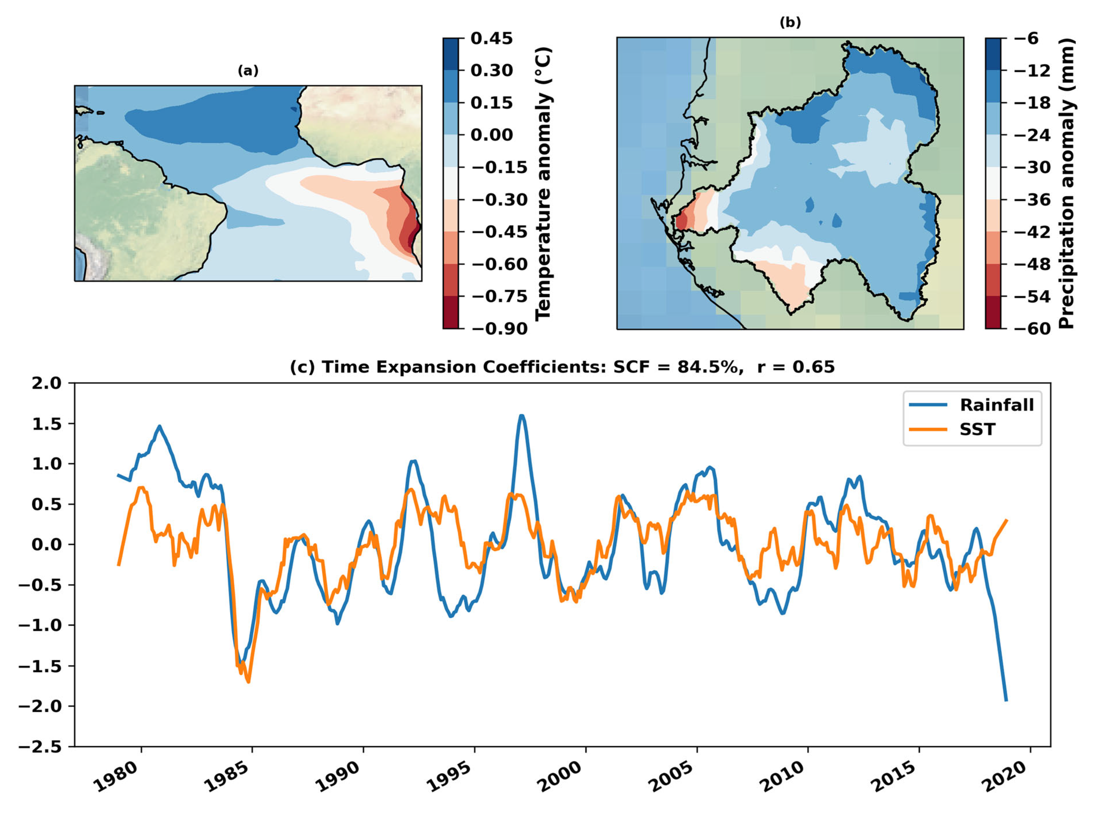
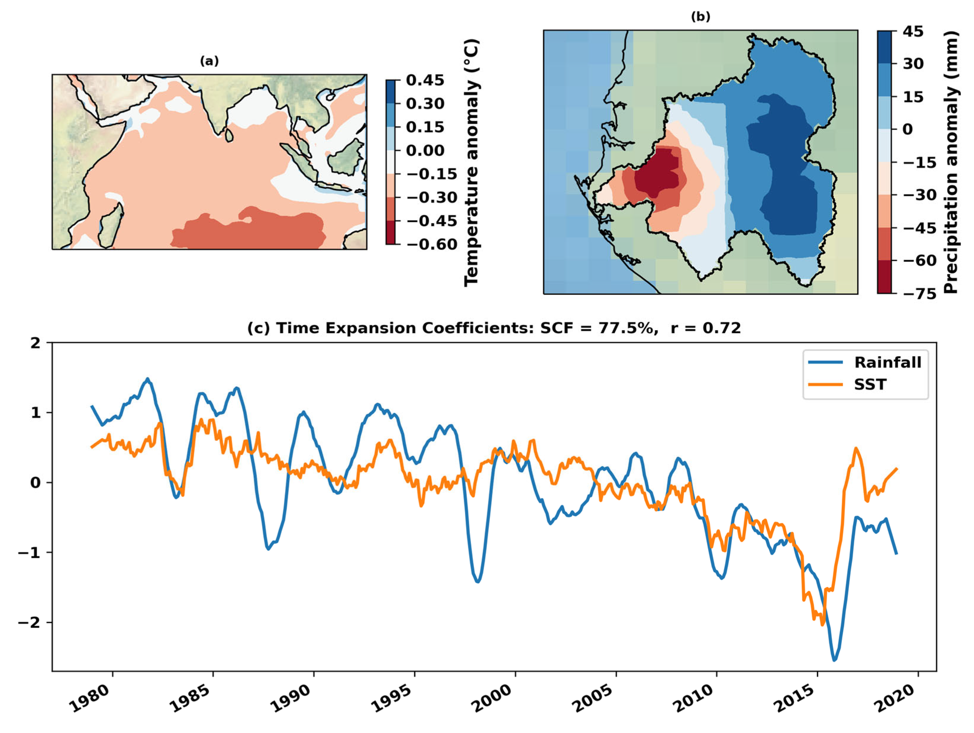
3.2. Coupled SST-Rainfall Patterns

This section presents the results of the MCA applied to the monthly MSWEP data from the ORB and the monthly TropFlux data from the three primary tropical ocean basins—the Pacific, Atlantic, and Indian Oceans—spanning the period from 1979 to 2018. It is important to highlight that the use of MCA to identify potential links between two geophysical fields does not require spatial harmonization of the data representing these fields. The only requirement is that the temporal extent of the data must be identical, as previously noted regarding the dimensions of the matrices used in the MCA.

Figure 3 shows the MCA-derived coupled patterns of SST in the Atlantic Ocean and rainfall in the ORB. The Atlantic SST pattern presents a strong signal along the coastal eastern equatorial area, with an extension along the Equator. Because of the similarities with the ENSO phenomenon in the Pacific, this pattern is often referred to as Atlantic Niño [71,72,73]. Considering the opposite SST anomalies on the northern part, along the coasts of Senegal and Mauritania, with a large expansion offshore, the whole tropical Atlantic pattern is more similar to the Atlantic Meridional Mode (AMM) [74,75,76]. The ORB rainfall pattern shows negative anomalies in the entire basin, with strong anomalies in the coastal region of the basin and decreasing anomalies upstream. These coupled patterns denoted the co-variation in rainfall in the whole ORB and SST in the tropical Atlantic Ocean, especially in the southeastern equatorial area. In addition, the squared covariance fraction for this maximum covariance pattern is 84%, denoting that the link between tropical SST in the Atlantic Ocean and rainfall in the ORB is almost totally represented in this first mode. Figure 3c shows the Time Expansion Coefficients (TEC) associated with the two SST-rainfall patterns. Both time series were filtered based on the Savitzky–Golay filter with 1-year window size to extract high-frequency noises that can hinder the correlation of these signals [77,78,79]. The computed Pearson correlation of both TECs is 0.69 (p-values < 0.05), significant at a 95% confidence level.

Figure 4 shows the coupled patterns resulting in the MCA of rainfall in the ORB and SST in the tropical Pacific Ocean. The SST pattern shows strong anomalies in the Pacific Ocean’s central to eastern equatorial area. SST anomalies in this area are usually associated with El Niño-Southern Oscillation (ENSO) [80,81,82]. In turn, the rainfall pattern in the ORB presents positive anomalies across the entire ORB. The most important anomalies are observed in the savanna zone of southeast ORB along the plateau Batéké. These anomalies decrease towards the north of the basin, as well as towards the west of the basin, with the lowest anomalies at the outlet of the basin downstream of Lambaréné. With a corresponding SCF of about 76.5%, this first mode of MCA between rainfall in the ORB and SST in the tropical Pacific Ocean represents its essential co-variation. These patterns show the common variation in rainfall in the ORB and ENSO in the Pacific Ocean. Numerous studies pointed out close-dependent variations of rainfall in the ORB and ENSO [13,30,31,83]. TECs associated with both patterns are shown in Figure 4c. These TECs were also filtered using the Savitzky–Golay filter with a 1-year window size to extract high-frequency noises. The Pearson correlation of both TECs is 0.49 (p < 0.05), and it is significant at a 95% significance level, denoting close co-variation in rainfall in the ORB and ENSO.

Figure 5 shows coupled patterns of SST in the tropical Indian Ocean and rainfall in the ORB. The associated Indian Ocean SST presents positive SST anomalies in almost the entire tropical Indian Ocean, with slightly stronger SST anomalies to the southeast of the ocean basin. Inversely, the associated ORB rainfall pattern shows positive (negative) anomalies in the east (west) of the ORB. This result is in agreement with those of other authors who have shown that variations in spring and autumn rainfall on the west coast of equatorial Africa, including the ORB, are influenced by SST throughout the whole tropical Indian Ocean [30,31]. Both patterns denote increasing (decreasing) rainfall in the east (west) of the ORB, related to positive SST anomalies in the tropical Indian Ocean. This first MCA mode between rainfall in the ORB and SST in the tropical Indian Ocean almost embeds the overall co-variation in these two geophysical fields, as its SCF is 77%. The TECs associated with these coupled patterns were filtered using the Savitzky–Golay filter with a 1-year window size and represented in Figure 5c. The computed Pearson correlation of both of these TECs resulted in 0.73 (p-value < 0.05), significant at a 95% significance level.

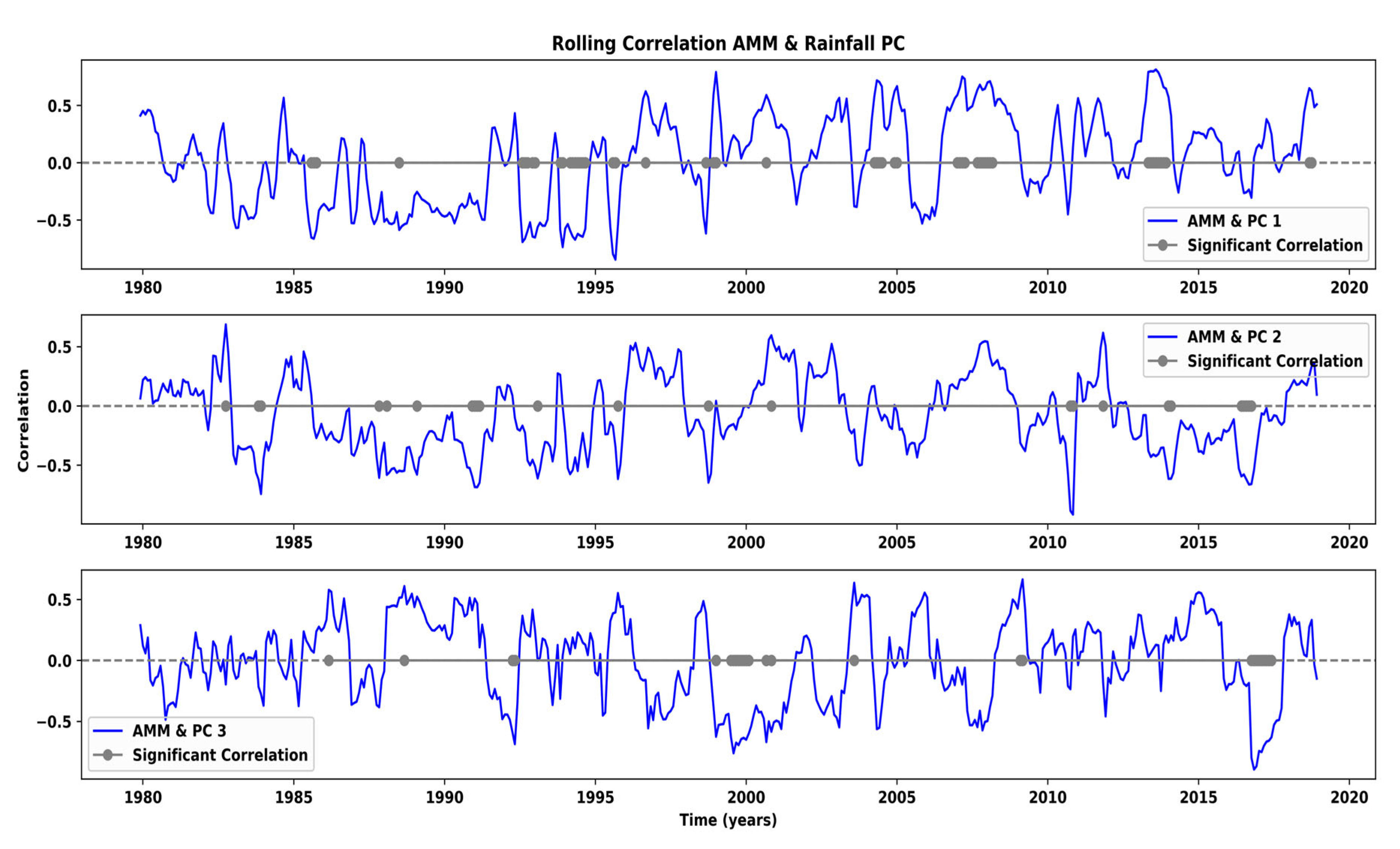
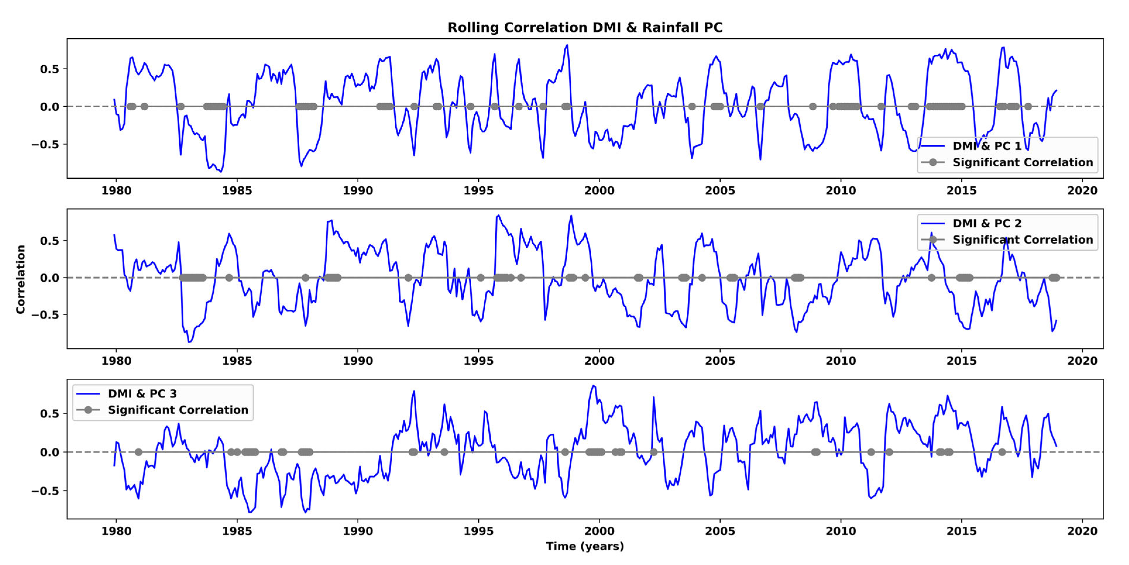
3.3. Relationships Between Rainfall in the ORB and SST in Tropical Oceans

The results of the time-dependent correlation analysis between the first PCs of the ORB rainfall and the climate indices whose links with rainfall were established from the MCA between the first of the ORB rainfall and the SST in the tropical ocean basins are presented in Figure 6, Figure 7 and Figure 8 below. The blue solid curves show the variations of the 1-year rolling window time-dependent correlation values as a function of time and the gray points indicate the times when the correlations are significant at the 95% confidence level. Overall, we note that these correlations very often oscillate between positive and negative values whatever the climate index or the mode of variation in rainfall considered in the ORB. These fluctuations between positive and negative correlations indicate that the climate index’s influence on ORB precipitation varies over time. During certain periods, the index may create conditions that enhance rainfall (e.g., by increasing moisture convergence over the ORB). Conversely, at other times, it may contribute to a reduction in precipitation (e.g., by suppressing convection or shifting storm tracks) [13,83]. However, understanding the actual mechanisms that control the relationship between climate indices and rainfall in the ORB, as well as in the broader Central African region, remains a complex research challenge due to the multitude of factors influencing precipitation in this area [27,28].

Figure 6 illustrates the dynamic relationships over time between the Atlantic Meridional Mode (AMM) index and the dominant modes of rainfall in the ORB region, using time-dependent correlations. This representation highlights periods where correlations are stronger, both positive and negative, with values greater than 0.5 and less than −0.5, respectively. There are gray dots placed on the graph indicating statistically significant correlations, verified at the 95% confidence level. These significant correlations reflect a marked co-variability between SST associated with the AMM mode and the main modes of rainfall in the ORB region. In particular, the rolling correlation with the first principal component (PC1), which explains 57% of the variance in ORB rainfall, shows significant periods, mainly concentrated in the last three decades of the study. This suggests the increasing influence of this mode over time.

Although less frequent, significant correlations with the second (PC2) and third principal component (PC3) are also observed over the entire study period, but these relationships remain globally less marked than those of PC1. This observation suggests that the interaction between AMM-related SST and the other precipitation modes, while significant, do not reach the same intensity or regularity as that observed with PC1. These results highlight a trend towards a greater influence of AMM on rainfall variations in the ORB region, particularly in recent decades, which could be related to regional climate change or other environmental phenomena affecting rainfall variability [45].

Figure 7 explores the dynamic relationship between the El Niño-Southern Oscillation (ENSO), represented by the Niño 3.4 index, and the principal components (PCs) of rainfall variability in the Ogooué River Basin (ORB). The figure displays rolling correlations, revealing substantial fluctuations between periods of strong correlation and decorrelation. This is evidenced by the abundance of gray dots, which denote statistically significant correlations at the 95% confidence level. The magnitude of these correlation values underscores their significance. The consistent presence of significant correlations, particularly with PC1, strongly suggests that the dominant mode of ORB rainfall variation is heavily influenced by ENSO activity in the tropical Pacific. While the rolling correlations between the Niño 3.4 index and PC2 and PC3 exhibit slightly fewer instances of statistical significance compared to PC1, the periods of notable correlation remain substantial. Crucially, the presence of both significant positive and negative correlations indicates that ENSO’s strong influence on ORB rainfall variability manifests during both the warm (El Niño) and cold (La Niña) phases of the oscillation. This suggests a complex and multifaceted interaction, where both El Niño and La Niña events can significantly modulate rainfall patterns in the ORB, albeit potentially in different ways. Further investigation is needed to fully characterize the specific impacts of each ENSO phase on ORB rainfall dynamics [13,29,30,31,44,83,84].

Figure 8 provides a detailed representation of the estimated rolling correlations between IDM index and the first three PCs of ORB rainfall variability. In contrast to the consistently significant correlations observed with ENSO index throughout most of the study period, the gray dots, which represent significant correlations, appear scattered for the IDM index. While the AMM and ENSO index exhibit significant correlations that are largely concentrated within specific periods, the significant correlations between IDM and ORB rainfall are more evenly distributed throughout the entire study duration. This suggests that the Indian Ocean Dipole (IOD) has an ongoing and more persistent influence on ORB rainfall, occurring across a broad range of years rather than being limited to isolated intervals.

Notably, these significant correlations, which manifest in distinct phases approximately every five years, highlight the periodic nature of the IOD’s influence on ORB rainfall variability. The recurring cycles, with frequencies of less than five within the study period, underscore the intermittent but notable impact of the IOD on the regional climate system. The positive and negative correlations shown in Figure 8 further reveal that the influence of the IDM on ORB rainfall is bidirectional—meaning that it exerts an effect during both its positive and negative phases. This dynamic interaction between the IDM and ORB rainfall underscores the complexity of the underlying mechanisms driving regional climate variability, and the findings suggest that the IOD plays a crucial role in shaping ORB rainfall patterns over extended periods [12,30,31].

4. Discussion

Some past studies have initiated this work of identifying the factors that influence rainfall in the ORB or larger areas, including the basin [13,29,30,31,44,83,84]. These studies were carried out using different statistical approaches, ranging from simple correlations to more complex techniques such as EOT and cross-wavelet analysis. This made it possible to highlight links between ORB rainfall and SST variations in the oceans, and many other factors. In the continuity, the present study uses the MCA to highlight the SST patterns in the tropical oceans, which influence the rainfall variations in the ORB. Improving upon previous studies, the use of MCA made it possible to determine the main modes of SST variability in the three large tropical ocean basins, which strongly influence the variability of most of the ORB. It should especially be noted that the first SST modes of the tropical oceans, which were coupled to the rainfall patterns in the ORB through the MCA, present squared covariance fractions that are close to 80%. This statistical metric is widely used in the domain of coupled geophysical fields to provide the measurement of the variability shared between two variables [60,85,86]. The tremendous values of the SCF guarantee very strong co-variations in the determined coupled patterns and do not share them with more than the 500 pairs of remaining patterns, explaining why the other modes are not considered in this study.

Another very important metric for understanding the relationships between the patterns obtained from the MCA is the correlation of the TECs associated with each mode [86]. It must be said that, even if the MCA makes it possible to highlight the dynamic modes with the most shared variance over time, the direct correlation of the TECs associated with each of the modes obtained is not guaranteed. In the application of MCA, TECs represent the temporal dynamics of modes individually and are not necessarily the direct relationship between them [42,86]. Thus, one often observes weak correlations or even decorrelations. In the present case, the correlations obtained from the TECs were relatively weak, although they are significant at the 95% confidence level as shown in

Table 1. Correlations of TECs.

TECs	Before Savitzky–Golay Filter	After Savitzky–Golay Filter
Atlantic Ocean	0.4	0.65
Pacific Ocean	0.23	0.5
Indian Ocean	0.43	0.72

. On the other hand, the application of the Savitzky–Golay filter on the TECs, which made it possible to reduce the high-frequency fluctuations of the latter, made more use of the shared co-variation while significantly improving the correlations as shown in Table 1 [86,87]. This supports the nonlinear relationships between the variations of the SST in the tropical oceans and rainfall variations in the ORB highlighted in the literature, as found in previous studies [13,83].

The use of time-dependent correlation analysis in this study has helped to highlight all the co-variations shared by the main modes of SST variations in the tropical oceans and those of rainfall in the ORB. Given the non-linearity of links highlighted with the MCA, and to remove any ambiguity in the interpretation of the teleconnections determined in this study, it was necessary to do better than the traditional correlation analysis which offers a single value representing the overall strength and direction of the relationship studied. Time-dependent correlation analysis is a technique that goes beyond this, offering a more detailed overview of the relationships between the variables studied. The periodically significant correlations shown in Figure 7 demonstrate the intermittent links between rainfall in the ORB and SST variations in the tropical Pacific Ocean through ENSO, which is the main mode of SST variability in this area [13,83]. In contrast, the idea generally put forward of a direct and permanent link between rainfall on the equatorial Atlantic coast of Africa and the tropical Atlantic Ocean, notably through its SST, the correlation between the AMM and ORB rainfall is intermittent, as can be seen in Figure 6, where the correlation is only significant at certain periods and, even then, irregularly. Given the MCA result with an SCF of 84% between tropical Atlantic and ORB rainfall, it is reasonable to assume that the link between both variables is also intermittent as with ENSO [36,72].

Inversely, even with MCA resulting in an SCF of 77.5% and a TEC correlation of 0.72, which indicates a strong link between tropical Indian Ocean SST variation and rainfall in the ORB, the Indian Ocean SST pattern shown in Figure 5a does not display the east–west contrast characteristic of the IDM [88]. This result is completely at odds with many previous studies on rainfall in central equatorial Africa which often consider IDM as the main mode of variability in the Indian Ocean and, above all, with a major influence on rainfall variability in equatorial Africa up to the western Atlantic coast [7,12,34,51,52,89]. Time-dependent correction analysis shows in Figure 8 that there is a clear link between rainfall in the ORB and IDM; although, as with the tropical basins of the Atlantic and Pacific Oceans, this link is only valid during specific periods. On the other hand, the periodically significant correlations demonstrate the non-linear nature of the links found above and go some way to justify the low correlations obtained from the TECs without the Savitzky–Golay filter, as shown in Table 1 and previously in [13,83].

The ORB rainfall regime is shaped by a complex interplay of climatic drivers, notably including sea surface temperatures (SSTs) in the tropical oceans. These SSTs primarily exert influence by modulating large-scale atmospheric circulation patterns, which subsequently govern moisture transport and precipitation over the basin and surrounding areas [29,90,91]. While the Atlantic, Indian, and Pacific Oceans all contribute to the ORB’s rainfall dynamics, their influences are distinct and multifaceted. These influences are further modulated by larger-scale climate systems, such as ENSO in the Pacific, IOD in the Indian, and AMM in the Atlantic. The interconnected nature of these systems means their fluctuations can either constructively interfere (amplifying rainfall variations) or destructively interfere (mitigating them), depending on the phase of each oscillation [91,92]. Despite the differing physical characteristics of each ocean basin, they can drive similar atmospheric responses through teleconnections. SST anomalies in one basin can trigger changes in global atmospheric circulation, with downstream effects impacting multiple regions, including the ORB. For example, Pacific Ocean SST anomalies associated with ENSO can influence the position and intensity of the Intertropical Convergence Zone (ITCZ), a key driver of seasonal rainfall in Central Africa, including the ORB [93]. Furthermore, Indian Ocean SST anomalies can influence the strength of the African Easterly Jet, affecting moisture transport from the Indian Ocean. Similarly, the AMM in the Atlantic can influence the strength of the West African Monsoon, which also affects the ORB’s rainfall [90,94]. Disentangling these complex interactions and quantifying the relative contributions of each ocean basin remains a significant challenge in understanding ORB rainfall variability.

5. Conclusions

This study investigated teleconnections between SSTs in the three major tropical ocean basins (Pacific, Atlantic, and Indian) and rainfall in the ORB using MCA. MCA revealed three coupled patterns between SSTs and ORB rainfall, exhibiting strong teleconnections evidenced by substantial SCFs of 76.5%, 77.5%, and 84% (all near 80%). Applying a Savitzky–Golay filter to the time series enhanced the clarity of these relationships, revealing strong correlations between the TECs of the identified coupled patterns. These correlations, with values exceeding 0.5 (0.5 for the Pacific, 0.7 for the Atlantic, and 0.73 for the Indian Ocean), are particularly noteworthy given the complex and often non-linear nature of teleconnections.

While MCA effectively highlighted coupled patterns and strong correlations, its inherent limitations should be acknowledged. MCA is a linear technique and, as such, may not fully capture the potentially non-linear dynamics of the teleconnections between SSTs and ORB rainfall. Furthermore, while the time-dependent correlation analysis provided additional support for these connections, particularly highlighting the influence of the AMM, ENSO, and the IDM, the MCA failed to adequately represent the IDM itself. Although time-dependent analysis suggests a periodic influence of the IDM on ORB rainfall, the linear nature of MCA may have limited its ability to resolve this complex relationship. Additionally, this study focused on identifying coupled patterns but did not quantify the relative contribution of each ocean basin to ORB rainfall variability. Future research employing more sophisticated methodologies, such as non-linear techniques, and potentially incorporating other relevant climate variables, could address this gap and provide a more comprehensive understanding of the complex interplay between tropical ocean SSTs and ORB rainfall. Despite these limitations, this study provides valuable insights into the teleconnection patterns influencing ORB rainfall and lays a foundation for further investigation.

References

1. Lau, K.-M.; Lim, H. On the Dynamics of Equatorial Forcing of Climate Teleconnections. J. Atmos. Sci. 1984, 41, 161–176. [Google Scholar] [CrossRef]
2. Burnett, A. Teleconnections. In Encyclopedia of World Climatology; Oliver, J.E., Ed.; Springer: Dordrecht, The Netherlands, 2005; pp. 707–711. ISBN 9781402032660. [Google Scholar]
3. An, S.-I.; Wang, C.; Mechoso, C.R. Teleconnections in the Atmosphere. In Interacting Climates of Ocean Basins: Observations, Mechanisms, Predictability, and Impacts; Cambridge University Press: Cambridge, UK, 2020; pp. 54–88. [Google Scholar]
4. Van den Dool, H.M.; Saha, S.; Johansson, Å. Empirical Orthogonal Teleconnections. J. Clim. 2000, 13, 1421–1435. [Google Scholar] [CrossRef]
5. Amirudin, A.A.; Salimun, E.; Tangang, F.; Juneng, L.; Zuhairi, M. Differential Influences of Teleconnections from the Indian and Pacific Oceans on Rainfall Variability in Southeast Asia. Atmosphere 2020, 11, 886. [Google Scholar] [CrossRef]
6. Eabry, M.D.; Taschetto, A.S.; Maharaj, A.M.; Sen Gupta, A. What Determines the Lagged ENSO Response in the South-west Indian Ocean? Geophys. Res. Lett. 2021, 48, e2020GL091958. [Google Scholar] [CrossRef]
7. Farnsworth, A.; White, E.; Williams, C.J.R.; Black, E.; Kniveton, D.R. Understanding the Large Scale Driving Mechanisms of Rainfall Variability over Central Africa. In African Climate and Climate Change: Physical, Social and Political Perspectives; Williams, C.J.R., Kniveton, D.R., Eds.; Springer: Dordrecht, The Netherlands, 2011; pp. 101–122. ISBN 9789048138425. [Google Scholar]
8. Adarsh, S.; Janga Reddy, M. Links Between Global Climate Teleconnections and Indian Monsoon Rainfall. In Climate Change Signals and Response: A Strategic Knowledge Compendium for India; Venkataraman, C., Mishra, T., Ghosh, S., Karmakar, S., Eds.; Springer: Singapore, 2019; pp. 61–72. ISBN 9789811302800. [Google Scholar]
9. Cardil, A.; Rodrigues, M.; Tapia, M.; Barbero, R.; Ramírez, J.; Stoof, C.R.; Silva, C.A.; Mohan, M.; de-Miguel, S. Climate Teleconnections Modulate Global Burned Area. Nat. Commun. 2023, 14, 427. [Google Scholar] [CrossRef]
10. Alizadeh, O. A Review of ENSO Teleconnections at Present and under Future Global Warming. Wiley Interdiscip. Rev. Clim. Change 2024, 15, e861. [Google Scholar] [CrossRef]
11. Beniche, M.; Vialard, J.; Lengaigne, M.; Voldoire, A.; Srinivas, G.; Hall, N.M.J. A Distinct and Reproducible Teleconnection Pattern over North America during Extreme El Niño Events. Sci. Rep. 2024, 14, 2457. [Google Scholar] [CrossRef]
12. Jiang, Y.; Zhou, L.; Roundy, P.E.; Hua, W.; Raghavendra, A. Increasing Influence of Indian Ocean Dipole on Precipitation over Central Equatorial Africa. Geophys. Res. Lett. 2021, 48, e2020GL092370. [Google Scholar] [CrossRef]
13. Bogning, S.; Frappart, F.; Mahé, G.; Paris, A.; Onguene, R.; Blarel, F.; Niño, F.; Etame, J.; Braun, J.-J. Investigating Links between Rainfall Variations in the Ogooué River Basin and ENSO in the Pacific Ocean over the Period 1940–1999. Proc. Int. Assoc. Hydrol. Sci. 2021, 384, 181–186. [Google Scholar] [CrossRef]
14. Silva, F.N.; Vega-Oliveros, D.A.; Yan, X.; Flammini, A.; Menczer, F.; Radicchi, F.; Kravitz, B.; Fortunato, S. Detecting Climate Teleconnections with Granger Causality. Geophys. Res. Lett. 2021, 48, e2021GL094707. [Google Scholar] [CrossRef]
15. Döös, K.; Kjellsson, J.; Zika, J.; Laliberté, F.; Brodeau, L.; Campino, A.A. The Coupled Ocean–Atmosphere Hydrothermohaline Circulation. J. Clim. 2017, 30, 631–647. [Google Scholar] [CrossRef]
16. Trenberth, K.E. Poleward Heat Transports by the Atmosphere and Ocean. In The Changing Flow of Energy Through the Climate System; Cambridge University Press: Cambridge, UK, 2022; pp. 121–139. [Google Scholar]
17. Tsonis, A.A.; Swanson, K.L.; Wang, G. On the Role of Atmospheric Teleconnections in Climate. J. Clim. 2008, 21, 2990–3001. [Google Scholar] [CrossRef]
18. Bonner, S.J.; Newlands, N.K.; Heckman, N.E. Modeling Regional Impacts of Climate Teleconnections Using Functional Data Analysis. Environ. Ecol. Stat. 2014, 21, 1–26. [Google Scholar] [CrossRef]
19. Liu, T.; Chen, D.; Yang, L.; Meng, J.; Wang, Z.; Ludescher, J.; Fan, J.; Yang, S.; Chen, D.; Kurths, J.; et al. Teleconnections among Tipping Elements in the Earth System. Nat. Clim. Change 2023, 13, 67–74. [Google Scholar] [CrossRef]
20. Rezaei, A.; Karami, K.; Tilmes, S.; Moore, J.C. Changes in Global Teleconnection Patterns under Global Warming and Stratospheric Aerosol Intervention Scenarios. Atmos. Chem. Phys. 2023, 23, 5835–5850. [Google Scholar] [CrossRef]
21. Hausfather, Z.; Marvel, K.; Schmidt, G.A.; Nielsen-Gammon, J.W.; Zelinka, M. Climate Simulations: Recognize the “Hot Model” Problem. Nature 2022, 605, 26–29. [Google Scholar] [CrossRef]
22. Schmidt, G. Climate Models Can’t Explain 2023’s Huge Heat Anomaly—We Could Be in Uncharted Territory. Nature 2024, 627, 467. [Google Scholar] [CrossRef]
23. Gutiérrez, O.; Panario, D.; Nagy, G.J.; Bidegain, M.; Montes, C. Climate Teleconnections and Indicators of Coastal Systems Response. Ocean Coast. Manag. 2016, 122, 64–76. [Google Scholar] [CrossRef]
24. Steptoe, H.; Jones, S.E.O.; Fox, H. Correlations between Extreme Atmospheric Hazards and Global Teleconnections: Implications for Multihazard Resilience. Rev. Geophys. 2018, 56, 50–78. [Google Scholar] [CrossRef]
25. Abtew, W.; Melesse, A.M. Climate Teleconnections and Water Management. In Nile River Basin: Ecohydrological Challenges, Climate Change and Hydropolitics; Melesse, A.M., Abtew, W., Setegn, S.G., Eds.; Springer International Publishing: Cham, Switzerland, 2014; pp. 685–705. ISBN 9783319027203. [Google Scholar]
26. Craig, P.M.; Allan, R.P. The Role of Teleconnection Patterns in the Variability and Trends of Growing Season Indices across Europe. Int. J. Climatol. 2022, 42, 1072–1091. [Google Scholar] [CrossRef]
27. Alsdorf, D.; Beighley, E.; Laraque, A.; Lee, H.; Tshimanga, R.; O’Loughlin, F.; Mahé, G.; Dinga, B.; Moukandi, G.; Spencer, R.G.M. Opportunities for Hydrologic Research in the Congo Basin. Rev. Geophys. 2016, 54, 378–409. [Google Scholar] [CrossRef]
28. Nicholson, S.E.; Funk, C.; Fink, A.H. Rainfall over the African Continent from the 19th through the 21st Century. Glob. Planet. Change 2018, 165, 114–127. [Google Scholar] [CrossRef]
29. Balas, N.; Nicholson, S.E.; Klotter, D. The Relationship of Rainfall Variability in West Central Africa to Sea-Surface Temperature Fluctuations. Int. J. Climatol. 2007, 27, 1335–1349. [Google Scholar] [CrossRef]
30. Dezfuli, A.K.; Nicholson, S.E. The Relationship of Rainfall Variability in Western Equatorial Africa to the Tropical Oceans and Atmospheric Circulation. Part II: The Boreal Autumn. J. Clim. 2013, 26, 66–84. [Google Scholar] [CrossRef]
31. Nicholson, S.E.; Dezfuli, A.K. The Relationship of Rainfall Variability in Western Equatorial Africa to the Tropical Oceans and Atmospheric Circulation. Part I: The Boreal Spring. J. Clim. 2013, 26, 45–65. [Google Scholar] [CrossRef]
32. Longandjo, G.-N.; Rouault, M. Revisiting the Seasonal Cycle of Rainfall over Central Africa. J. Clim. 2024, 37, 1015–1032. [Google Scholar] [CrossRef]
33. Balas, N. Climatic Variability in Central Africa and Its Link to Sea Surface Temperature and the El Nino/la Nina. 2003. Available online: https://repository.lib.fsu.edu/islandora/object/fsu:169208 (accessed on 27 February 2025).
34. Moihamette, F.; Pokam, W.M.; Diallo, I.; Washington, R. Extreme Indian Ocean Dipole and Rainfall Variability over Central Africa. Int. J. Climatol. 2022, 42, 5255–5272. [Google Scholar] [CrossRef]
35. Moihamette, F.; Pokam, W.M.; Diallo, I.; Washington, R. Response of Regional Circulation Features to the Indian Ocean Dipole and Influence on Central Africa Climate. Clim. Dyn. 2024, 62, 1–21. [Google Scholar] [CrossRef]
36. Lüdecke, H.-J.; Müller-Plath, G.; Wallace, M.G.; Lüning, S. Decadal and Multidecadal Natural Variability of African Rainfall. J. Hydrol. Reg. Stud. 2021, 34, 100795. [Google Scholar] [CrossRef]
37. Ebodé, V.B. Analysis of the Spatio-Temporal Rainfall Variability in Cameroon over the Period 1950 to 2019. Atmosphere 2022, 13, 1769. [Google Scholar] [CrossRef]
38. Wamba Tchinda, C.; Tchakoutio Sandjon, A.; Djiotang Tchotchou, A.L.; Nzeudeu Siwe, A.; Vondou, D.A.; Nzeukou, A. The Influence of Intraseasonal Oscillations on Rainfall Variability over Central Africa: Case of the 25–70 Days Variability. Sci. Rep. 2023, 13, 19842. [Google Scholar] [CrossRef] [PubMed]
39. Raghavendra, A.; Xia, G.; Zhou, L.; Jiang, Y. Orographic Enhancement of Rainfall over the Congo Basin. Atmos. Sci. Lett. 2022, 23, e1079. [Google Scholar] [CrossRef]
40. Wallace, J.M.; Smith, C.; Bretherton, C.S. Singular Value Decomposition of Wintertime Sea Surface Temperature and 500-Mb Height Anomalies. J. Clim. 1992, 5, 561–576. [Google Scholar] [CrossRef]
41. Cherry, S. Singular Value Decomposition Analysis and Canonical Correlation Analysis. J. Clim. 1996, 9, 2003–2009. [Google Scholar] [CrossRef]
42. Cherry, S. Some Comments on Singular Value Decomposition Analysis. J. Clim. 1997, 10, 1759–1761. [Google Scholar] [CrossRef]
43. Mignard, S.L.-A.; Mulder, T.; Martinez, P.; Charlier, K.; Rossignol, L.; Garlan, T. Deep-Sea Terrigenous Organic Carbon Transfer and Accumulation: Impact of Sea-Level Variations and Sedimentation Processes off the Ogooue River (Gabon). Mar. Pet. Geol. 2017, 85, 35–53. [Google Scholar] [CrossRef]
44. Mahé, G.; Lerique, J.; Olivry, J.-C. Le Fleuve Ogooué au Gabon: Reconstitution des Débits Manquants et Mise en Évidence de Variations Climatiques à L’Équateur. 1990. Available online: https://agris.fao.org/search/en/providers/122415/records/647368a92c1d629bc9805563 (accessed on 27 February 2025).
45. Bogning, S.; Frappart, F.; Mahé, G.; Niño, F.; Paris, A.; Sihon, J.; Ghomsi, F.; Blarel, F.; Bricquet, J.-P.; Onguene, R.; et al. Long-term Hydrological Variations of the Ogooué River Basin. In Congo Basin Hydrology, Climate, and Biogeochemistry; Wiley: Hoboken, NJ, USA, 2022; pp. 367–389. [Google Scholar]
46. Bedigian, D. Gamba, Gabon: Biodiversité D’une Forêt équatoriale Africane [Gamba, Gamboa: Biodiversity of an Equatorial African Rainforest. Econ. Bot. 2007, 61, 104. [Google Scholar]
47. Nieto-Quintano, P.; Mitchard, E.T.A.; Odende, R.; Batsa Mouwembe, M.A.; Rayden, T.; Ryan, C.M. The Mesic Savannas of the Bateke Plateau: Carbon Stocks and Floristic Composition. Biotropica 2018, 50, 868–880. [Google Scholar] [CrossRef]
48. Martin, D.; Chatelin, Y.; Collinet, J.; Guichard, E.; Sala, G.-H.; Le Rouget, G. Les Sols du Gabon: Pédogenèse, Répartition et Aptitudes: Cartes à 1:2.000.000; ORSTOM: Paris, France, 1981; ISBN 9782709906142. [Google Scholar]
49. Kittel, C.M.M.; Nielsen, K.; Tøttrup, C.; Bauer-Gottwein, P. Informing a Hydrological Model of the Ogooué with Multi-Mission Remote Sensing Data. Hydrol. Earth Syst. Sci. 2018, 22, 1453–1472. [Google Scholar] [CrossRef]
50. Giresse, P. Esquisse Géologique de l’Afrique Centrale Occidentale. In Paysages Quaternaires de l’Afrique Centrale Occidentale; ORSTOM: Paris, France, 1990; pp. 15–19. ISBN 9782709910224. [Google Scholar]
51. Hua, W.; Zhou, L.; Chen, H.; Nicholson, S.E.; Raghavendra, A.; Jiang, Y. Possible Causes of the Central Equatorial African Long-Term Drought. Environ. Res. Lett. 2016, 11, 124002. [Google Scholar] [CrossRef]
52. Diem, J.E.; Salerno, J.D.; Palace, M.W.; Bailey, K.; Hartter, J. Teleconnections between Rainfall in Equatorial Africa and Tropical Sea Surface Temperatures: A Focus on Western Uganda. J. Appl. Meteorol. Climatol. 2021, 60, 967–979. [Google Scholar] [CrossRef]
53. Swain, S.; Patel, P.; Nandi, S. Application of SPI, EDI and PNPI Using MSWEP Precipitation Data over Marathwada, India. In Proceedings of the 2017 IEEE International Geoscience and Remote Sensing Symposium (IGARSS), Fort Worth, TX, USA, 23–28 July 2017; IEEE: Piscataway, NJ, USA, 2017; pp. 5505–5507. [Google Scholar]
54. Satgé, F.; Defrance, D.; Sultan, B.; Bonnet, M.-P.; Seyler, F.; Rouché, N.; Pierron, F.; Paturel, J.-E. Evaluation of 23 Gridded Precipitation Datasets across West Africa. J. Hydrol. 2020, 581, 124412. [Google Scholar] [CrossRef]
55. Beck, H.E.; van Dijk, A.I.J.M.; Levizzani, V.; Schellekens, J.; Miralles, D.G.; Martens, B.; de Roo, A. MSWEP: 3-Hourly 0.25° Global Gridded Precipitation (1979–2015) by Merging Gauge, Satellite, and Reanalysis Data. Hydrol. Earth Syst. Sci. 2017, 21, 589–615. [Google Scholar] [CrossRef]
56. Beck, H.E.; Wood, E.F.; Pan, M.; Fisher, C.K.; Miralles, D.G.; Van Dijk, A.I.; McVicar, T.R.; Adler, R.F. MSWEP V2 Global 3-Hourly 0.1 Precipitation: Methodology and Quantitative Assessment. Bull. Am. Meteorol. Soc. 2019, 100, 473–500. [Google Scholar] [CrossRef]
57. Aniley, E.; Gashaw, T.; Abraham, T.; Demessie, S.F.; Bayabil, H.K.; Worqlul, A.W.; van Oel, P.R.; Dile, Y.T.; Chukalla, A.D.; Haileslassie, A.; et al. Evaluating the Performances of Gridded Satellite/reanalysis Products in Representing the Rainfall Climatology of Ethiopia. Geocarto Int. 2023, 38, 2278329. [Google Scholar] [CrossRef]
58. Praveen Kumar, B.; Vialard, J.; Lengaigne, M.; Murty, V.S.N.; McPhaden, M.J. TropFlux: Air-Sea Fluxes for the Global Tropical Oceans—Description and Evaluation. Clim. Dyn. 2012, 38, 1521–1543. [Google Scholar] [CrossRef]
59. Frankignoul, C.; Chouaib, N.; Liu, Z. Estimating the Observed Atmospheric Response to SST Anomalies: Maximum Covariance Analysis, Generalized Equilibrium Feedback Assessment, and Maximum Response Estimation. J. Clim. 2011, 24, 2523–2539. [Google Scholar] [CrossRef]
60. Barreto, N.J.C.; Mesquita, M.d.S.; Mendes, D.; Spyrides, M.H.C.; Pedra, G.U.; Lucio, P.S. Maximum Covariance Analysis to Identify Intraseasonal Oscillations over Tropical Brazil. Clim. Dyn. 2017, 49, 1583–1596. [Google Scholar] [CrossRef]
61. Bretherton, C.S.; Smith, C.; Wallace, J.M. An Intercomparison of Methods for Finding Coupled Patterns in Climate Data. J. Clim. 1992, 5, 541–560. [Google Scholar] [CrossRef]
62. Levine, R.C.; Turner, A.G.; Marathayil, D.; Martin, G.M. The Role of Northern Arabian Sea Surface Temperature Biases in CMIP5 Model Simulations and Future Projections of Indian Summer Monsoon Rainfall. Clim. Dyn. 2013, 41, 155–172. [Google Scholar] [CrossRef]
63. Polanco-Martínez, J.M.; López-Martínez, J.L. NonParRolCor: An R Package for Estimating Rolling Correlation for Two Regular Time Series. SoftwareX 2023, 22, 101353. [Google Scholar] [CrossRef]
64. McMillan, D.G. The Time-Varying Relation between Stock Returns and Monetary Variables. J. Risk Financ. Manag. 2021, 15, 9. [Google Scholar] [CrossRef]
65. Litzow, M.A.; Ciannelli, L.; Puerta, P.; Wettstein, J.J.; Rykaczewski, R.R.; Opiekun, M. Nonstationary Environmental and Community Relationships in the North Pacific Ocean. Ecology 2019, 100, e02760. [Google Scholar] [CrossRef] [PubMed]
66. Rahman, M.; Islam, M.; Wernicke, J.; Bräuning, A. Changes in Sensitivity of Tree-Ring Widths to Climate in a Tropical Moist Forest Tree in Bangladesh. Forests 2018, 9, 761. [Google Scholar] [CrossRef]
67. Salem, N.; Hussein, S. Data Dimensional Reduction and Principal Components Analysis. Procedia Comput. Sci. 2019, 163, 292–299. [Google Scholar] [CrossRef]
68. Singh, C.V. Pattern Characteristics of Indian Monsoon Rainfall Using Principal Component Analysis (PCA). Atmos. Res. 2006, 79, 317–326. [Google Scholar] [CrossRef]
69. Cerón, W.L.; Molina-Carpio, J.; Ayes Rivera, I.; Andreoli, R.V.; Kayano, M.T.; Canchala, T. A Principal Component Analysis Approach to Assess CHIRPS Precipitation Dataset for the Study of Climate Variability of the La Plata Basin, Southern South America. Nat. Hazards 2020, 103, 767–783. [Google Scholar] [CrossRef]
70. Lienou, G.; Mahe, G.; Paturel, J.E.; Servat, E.; Sighomnou, D.; Ekodeck, G.E.; Dezetter, A.; Dieulin, C. Evolution Des Régimes Hydrologiques En Région équatoriale Camerounaise: Un Impact de La Variabilité Climatique En Afrique équatoriale? Hydrol. Sci. J. 2008, 53, 789–801. [Google Scholar] [CrossRef]
71. Lübbecke, J.F.; Böning, C.W.; Keenlyside, N.S.; Xie, S.-P. On the Connection between Benguela and Equatorial Atlantic Niños and the Role of the South Atlantic Anticyclone. J. Geophys. Res. 2010, 115, 2293. [Google Scholar] [CrossRef]
72. Lutz, K.; Rathmann, J.; Jacobeit, J. Classification of Warm and Cold Water Events in the Eastern Tropical Atlantic Ocean. Atmos. Sci. Lett. 2013, 14, 102–106. [Google Scholar] [CrossRef]
73. Lübbecke, J.F.; McPhaden, M.J. Symmetry of the Atlantic Niño Mode. Geophys. Res. Lett. 2017, 44, 965–973. [Google Scholar] [CrossRef]
74. Xia, F.; Zuo, J.; Sun, C.; Liu, A. The Atlantic Meridional Mode and Associated Wind–SST Relationship in the CMIP6 Models. Atmosphere 2023, 14, 359. [Google Scholar] [CrossRef]
75. Hari, V.; Rakovec, O.; Zhang, W.; Koppa, A.; Collins, M.; Kumar, R. On the Role of the Atlantic Meridional Mode in Eastern European Temperature Variability. Atmos. Res. 2024, 297, 107082. [Google Scholar] [CrossRef]
76. Zhang, Q.; Chang, P.; Fu, D.; Yeager, S.G.; Danabasoglu, G.; Castruccio, F.; Rosenbloom, N. Enhanced Atlantic Meridional Mode Predictability in a High-Resolution Prediction System. Sci. Adv. 2024, 10, eado6298. [Google Scholar] [CrossRef]
77. Baba, K.; Bahi, L.; Ouadif, L. Enhancing Geophysical Signals Through the Use of Savitzky-Golay Filtering Method. Geofísica Int. 2014, 53, 399–409. [Google Scholar] [CrossRef]
78. Liu, Y.; Dang, B.; Li, Y.; Lin, H.; Ma, H. Applications of Savitzky-Golay Filter for Seismic Random Noise Reduction. Acta Geophys. 2016, 64, 101–124. [Google Scholar] [CrossRef]
79. Roy, I.G. An Optimal Savitzky–Golay Derivative Filter with Geophysical Applications: An Example of Self-potential Data. Geophys. Prospect. 2020, 68, 1041–1056. [Google Scholar] [CrossRef]
80. An, S.-I.; Wang, B. Mechanisms of Locking of the El Niño and La Niña Mature Phases to Boreal Winter. J. Clim. 2001, 14, 2164–2176. [Google Scholar] [CrossRef]
81. Santoso, A.; Mcphaden, M.J.; Cai, W. The Defining Characteristics of ENSO Extremes and the Strong 2015/2016 El Niño. Rev. Geophys. 2017, 55, 1079–1129. [Google Scholar] [CrossRef]
82. Jiang, S.; Zhu, C.; Jiang, N. Impacts of the Annual Cycle of Background SST in the Tropical Pacific on the Phase and Amplitude of ENSO. Atmos. Ocean. Sci. Lett. 2025, 18, 100496. [Google Scholar] [CrossRef]
83. Bogning, S.; Frappart, F.; Paris, A.; Blarel, F.; Niño, F. Hydro-Climatology Study of the Ogooué River Basin Using Hydrological Modeling and Satellite Altimetry. Adv. Space Res. 2021, 68, 672–690. [Google Scholar] [CrossRef]
84. Maloba Makanga, J.D. Variabilité Pluviométrique de La Petite Saison Sèche Au Gabon. In Proceedings of the XXVIIIe Colloque de l’Association Internationale de Climatologie, Liège, Belgium, 1–4 July 2015; Université de Liège: Liège, Belgium, 2015; p. 6. [Google Scholar]
85. An, S.-I. Conditional Maximum Covariance Analysis and Its Application to the Tropical Indian Ocean SST and Surface Wind Stress Anomalies. J. Clim. 2003, 16, 2932–2938. [Google Scholar] [CrossRef]
86. Riaz, S.M.F.; Iqbal, M.J.; Baig, M.J. Influence of Siberian High on Temperature Variability over Northern Areas of South Asia. Meteorol. Atmos. Phys. 2018, 130, 441–457. [Google Scholar] [CrossRef]
87. Joetzjer, E.; Douville, H.; Delire, C.; Ciais, P. Present-Day and Future Amazonian Precipitation in Global Climate Models: CMIP5 versus CMIP3. Clim. Dyn. 2013, 41, 2921–2936. [Google Scholar] [CrossRef]
88. Koesuma, S.; Andriani, R.D.; Legowo, B. Analyzing of the Indian Ocean Dipole (IOD) Phenomena in Relation to Climate Change in Indonesia: A Review. J. Phys. Conf. Ser. 2021, 1918, 022030. [Google Scholar] [CrossRef]
89. Jarugula, S.; McPhaden, M.J. Indian Ocean Dipole Affects Eastern Tropical Atlantic Salinity through Congo River Basin Hydrology. Commun. Earth Environ. 2023, 4, 366. [Google Scholar] [CrossRef]
90. Izumo, T.; Vialard, J.; Lengaigne, M.; Suresh, I. Relevance of Relative Sea Surface Temperature for Tropical Rainfall Interannual Variability. Geophys. Res. Lett. 2020, 47, e2019GL086182. [Google Scholar] [CrossRef]
91. Stuecker, M.F. The Climate Variability Trio: Stochastic Fluctuations, El Niño, and the Seasonal Cycle. Geosci. Lett. 2023, 10, 51. [Google Scholar] [CrossRef]
92. Pothapakula, P.K.; Primo, C.; Sørland, S.; Ahrens, B. The Synergistic Impact of ENSO and IOD on the Indian Summer Monsoon Rainfall in Observations and Climate Simulations—An Information Theory Perspective. Earth Syst. Dyn. Discuss. 2020, 11, 903–923. [Google Scholar] [CrossRef]
93. Crespo, L.R.; Keenlyside, N.; Koseki, S. The Role of Sea Surface Temperature in the Atmospheric Seasonal Cycle of the Equatorial Atlantic. Clim. Dyn. 2019, 52, 5927–5946. [Google Scholar] [CrossRef]
94. Zhang, G.; Chen, J.; Fan, H.; Zhang, L.; Chen, M.; Wang, X.; Wang, D. Unveiling the Role of South Tropical Atlantic in Winter Atlantic Niño Inducing La Niña. Nat. Commun. 2025, 16, 1612. [Google Scholar] [CrossRef]
Figure 1. Location map of the ORB with some details on the hydrographic network and topography.
Water 17 00753 g001
Figure 2. EOFs and associated temporal PCs from the PCA of rainfall of the ORB. The three leading modes of ORB rainfall variability (1979–2018), represented by EOFs, are depicted in the maps. The corresponding temporal principal components, showing the evolution of each mode over time, are plotted in curves.
Water 17 00753 g002
Figure 3. Primary mode of co-variability identified by MCA between monthly precipitation in the ORB and monthly sea SST in the tropical Atlantic Ocean. Maps (a,b) depict the coupled spatial patterns of SST and precipitation anomalies associated with this mode. Graphs (c) show the temporal evolution of the time expansion coefficients associated with these patterns, indicating their relative importance over time.
Water 17 00753 g003
Figure 4. Primary mode of co-variability identified by MCA between monthly precipitation in the ORB and monthly sea SST in the tropical Pacific Ocean. Maps (a,b) depict the coupled spatial patterns of SST and precipitation anomalies associated with this mode. Graphs (c) show the temporal evolution of the time expansion coefficients associated with these patterns, indicating their relative importance over time.
Water 17 00753 g004
Figure 5. Primary mode of co-variability identified by MCA between monthly precipitation in the ORB and monthly sea SST in the tropical Indian Ocean. Maps (a,b) depict the coupled spatial patterns of SST and precipitation anomalies associated with this mode. Graphs (c) show the temporal evolution of the time expansion coefficients associated with these patterns, indicating their relative importance over time.
Water 17 00753 g005
Figure 6. Moving correlation between AMM and the leading temporal PCs of rainfall in the ORB. Blue lines show 12-month rolling correlations with the principal components derived from the three leading EOFs. Gray dots indicate statistically significant correlations.
Water 17 00753 g006
Figure 7. Moving correlations between ENSO and leading temporal PCs of rainfall in the ORB. Blue lines show 12-month rolling correlations with the principal components derived from the three leading EOFs. Gray dots indicate statistically significant correlations.
Water 17 00753 g007
Figure 8. Moving correlations between IDM and leading temporal PCs of rainfall in the ORB. Blue lines show 12-month rolling correlations with the principal components derived from the three leading EOFs. Gray dots indicate statistically significant correlations.
Water 17 00753 g008