Article

Evaluating Modeling Approaches for Phytoplankton Productivity in Estuaries

1
Estuary and Ocean Science Center, Romberg Tiburon Campus, San Francisco State University, 3150 Paradise Drive, Tiburon, CA 94920, USA
2
Department of Sciences and Mathematics, California State University Maritime Academy, 200 Maritime Academy Drive, Vallejo, CA 94590, USA
*
Author to whom correspondence should be addressed.
Water 2025, 17(5), 747; https://doi.org/10.3390/w17050747
Submission received: 23 December 2024 / Revised: 27 February 2025 / Accepted: 1 March 2025 / Published: 4 March 2025
(This article belongs to the Section Biodiversity and Functionality of Aquatic Ecosystems)

Abstract

:
Phytoplankton comprise the base of the food web in estuaries and their biomass and rates of growth (productivity) exert a bottom-up control in pelagic ecosystems. Reliable means to quantify biomass and productivity are crucial for managing estuarine ecosystems. In many estuaries, direct productivity measurements are rare and instead are estimated with biomass-based models. A seminal example of this is a light utilization model (LUM) used to predict productivity in the San Francisco Estuary and Delta (SFED) from long timeseries data using an efficiency factor, ψ. Applications of the LUM in the SFED, Chesapeake Bay, and the Dutch Scheldt Estuary highlight significant interannual and regional variability, indicating the model must be recalibrated often. The objectives of this study are to revisit the LUM approach in the SFED and assess a chlorophyll-a to carbon model (CCM) that produces a tuning parameter, Ω. To assess the estimates of primary productivity resulting from the models, productivity was directly measured with a 13C-tracer at nine locations during 22 surveys using field-derived phytoplankton incubations between March and November of 2023. For this study, ψ was determined to be 0.42 ± 0.02 (r2 = 0.89, p < 0.001, CI95 = 319). Modeling productivity using an alternative CCM approach (Ω = 3.47 × 10⁴ ± 1.7 × 10³, r2 = 0.84, p < 0.001, CI95 = 375) compared well to the LUM approach, expanding the toolbox for estuarine researchers to cross-examine productivity models. One practical application of this study is that it confirms an observed decline in ψ, suggesting a decline in light utilization by phytoplankton in the SFED. This highlights the importance of occasionally recalibrating productivity models in estuaries and leveraging multiple modeling approaches to validate estimations before application in ecological management decision making.

1. Introduction

Phytoplankton productivity is important in supporting food webs and fishes of aquatic ecosystems, including wetlands. Worldwide and throughout history, wetlands have been claimed by humanity, chiefly for agriculture, freshwater resources, and inland shipping ports [1]. The associated pelagic ecosystems, which once relied on phytoplankton carbon from productive wetlands as a source of primary production, are now primarily dependent on phytoplankton carbon produced within less productive pelagic systems to support the base of estuarine food webs. This phenomenon is exemplified by the San Francisco Estuary and Delta (SFED, see Table 1 for acronyms) in California where between 77 and 85% of the wetlands have been reclaimed and irreversibly altered due to the allocation of land and water resources for agriculture [2,3]. Abundances of pelagic organisms in the SFED sharply declined after 2000, raising concerns from natural resource agencies that the food web was degrading [4]. This observation spurred decades of research into potential causes for the decline, one being chronically depressed phytoplankton biomass [5].
Enhanced phytoplankton biomass is one criterion by which ecosystem restoration can be assessed for success [6]. As a result, phytoplankton biomass monitoring is a staple among natural resource agencies and researchers. Typically, the monitoring of chlorophyll-a fluorescence, a common proxy for phytoplankton biomass, is conducted continuously by telemetered fluorometers (in vivo) and discretely through grab samples (in vitro). Chlorophyll-a fluorometry is cost effective; however, the metric is unable to explain if the biomass is growing or simply accumulating due to hydrodynamics [7]. For this reason, complementary direct measurements of phytoplankton primary productivity, the growth that supports the increase in biomass, are necessary to establish baseline data for interannual or regional comparisons and assess restoration success, ecosystem function, and food web resources. These rates can be measured from the uptake and incorporation of isotopic tracers (e.g., 13C, 14C) by phytoplankton or changes in oxygen during an incubation period [8,9]. Due to cost, technical, and time barriers for many agencies and researchers, these rates are rarely measured with direct approaches and instead are usually estimated from simple linear regression models utilizing phytoplankton biomass and other easily monitored parameters. Here, we use direct measurement techniques with isotopic tracers to evaluate two simple linear regression models for productivity in the SFED.
One such model that is widely used in the SFED is a linear regression known as the light utilization model (LUM) [5,10]. The LUM estimates photic zone daily net phytoplankton productivity (PNpd, also referred to as ∫P and ΣP in some publications) from chlorophyll-a and light availability. PNpd (mg-C m−2 d−1) is a measure of the uptake of carbon over a cross-section of a water column and is relevant to larger coupled hydrodynamic-ecological models [6]. This model was initially calibrated with direct measurements of phytoplankton productivity in the major saline embayments of the SFED in the 1980s [10]. Later calibrations were focused in the freshwater Delta [5] and ‘low salinity zone’ [11,12], which extends from San Pablo Bay to the Delta (Figure 1) depending on annual freshwater outflow. These studies each conducted a linear regression between measured PNpd and a composite parameter (BE0Zp) made from the product of chlorophyll-a concentration (B, mg-Chl m−3), ambient photosynthetically active radiation (E0, E m−2 d−1), and photic zone depth (Zp, m). The slope of the regression line—the efficiency factor (ψ)—is then used to predict PNpd from long running historical records of BE0Zp going forward (e.g., [3,5,13,14]). Another study [12] made its own determination of ψ and recalculated prior determinations of ψ in the SFED. The authors concluded that (1) the observed interannual variability in ψ detracts from its reliability as a general modeling approach on timeseries greater than one year and (2) continued effort should be aimed at making direct measurements of phytoplankton productivity in estuarine systems. Studies from other estuaries present mixed results but emphasize the first conclusion [15,16]. Still, the value of a reliable and simplistic model for phytoplankton productivity cannot be understated.
Another modeling approach, which, to our knowledge, is untested in estuaries, uses chlorophyll to phytoplankton carbon ratios (B:Cp) to predict PNpd. This modeling approach is referred to here as a chlorophyll-to-carbon model (CCM). The inspiration for this approach stems from the following observations. First, off of the coast of British Columbia, the lowest values of Cp:B (highest values of B:Cp) were constrained to the highly productive upwelling zone, and the highest values of Cp:B (lowest values of B:Cp) were constrained just seaward of the continental shelf, which are classically less productive [17]. Additionally, B:Cp ratios have been used to estimate the growth rate (µ) of phytoplankton assemblages and exhibit a dynamic relationship, with µ depending on light and nutrient resources in laboratory studies [18]. Intrigued, this research has the following aims: (1) to revisit the LUM and address recent conclusions about its general use in estuaries [12] and (2) evaluate the performance of the LUM in comparison to the performance of the CCM at retrieving observed phytoplankton primary productivity (PNpd) for estuaries. One novelty is to provide an alternative model for estimating estuarine productivity in areas where direct measurements are lacking.

2. Materials and Methods

2.1. Study Region Description

The SFED (Figure 1) is an urban estuary in central California, serving as the drain for 40% of the state’s acreage. The brackish northern SFED includes Suisun Bay, while further inland is the Delta, beginning at the confluence of the Sacramento and San Joaquin Rivers and roughly bounded northward by the Yolo Bypass (YB) floodplain. The majority of freshwater flow into the SFED originates during the winter and early spring in northern California and enters the SFED through the Sacramento River and Yolo Bypass floodplain. Freshwater flow into the SFED is mostly managed by upstream reservoirs. This research was conducted on a hydrological transect (Figure 1) consisting of nine monitoring stations. Five stations (I-80TD, LIS, STTD, BL5, and LIB) were along a slough known as the Toe Drain in the YB, and four stations (US655, US649, US5, DWR-D7) were within the northern San Francisco Estuary (nSFE), which encompasses Suisun Bay and the seaward portion of the Delta.

2.2. Sampling and Laboratory Methods

This research was conducted between 31 March and 2 November 2023, with the transect sampled during 22 ~biweekly surveys. When data were aggregated by months, 31 March was lumped with April dates to better calculate confidence intervals. Water samples from the nSFE stations US655, US649, US5, and DWR-D7 were collected aboard the R/V Questuary by deploying a Sea Bird Electronics SB-32 rosette fitted with four 3-L Niskin bottles and a Seabird SBE-19 plus CTD. This allowed for the collection of water samples at the near surface (<1 m) while also taking real-time vertical profiles of PAR. Secchi depths were measured in parallel with vertical PAR profiles. Water samples from the YB stations I-80TD, LIS, STTD, BL5, and LIB were collected at the near-surface by the California Department of Water Resources personnel from a boat using a Van Dorn Bottle or from land with a dip stick. Secchi depths were measured at all stations along the YB.
Water samples for the analysis of dissolved inorganic carbon (DIC) concentrations, necessary for calculating phytoplankton carbon uptake, were collected and analyzed using an MBARI clone DIC analyzer with acid sparging and non-dispersive infrared analysis [19]. For chlorophyll and nutrient concentration analyses, sample water was filtered through 25-mm Whatman GF/F filters, and the filter and filtrate were immediately put on ice during transit and then frozen. Filters were analyzed with a Turner Designs Model 10-AU fluorometer for chlorophyll-a concentrations with phaeophytin-a correction [20]. Filtrates were analyzed for ammonium, nitrate, nitrite, silicate, and phosphate. Ammonium samples were analyzed using spectrophotometry (10 cm path-length cell) [21]. Other nutrients were analyzed with a Bran and Luebbe AutoAnalyzer II with the MT-19 manifold chemistry module [22,23,24].
To measure phytoplankton carbon uptake, 150-mL clear polycarbonate incubation bottles were filled with sample water from each station and spiked with a trace amount of NaH13CO3 (99 at%) equivalent to ~10% of the ambient DIC concentration. Incubation bottles were placed into wire-screened, neutral density tubes or bags with a nominal shading percentage determined with a LI-COR Quantum Sensor (a dark bottle, 1, 3, 10, 25, and 70% of ambient irradiance) [11,25]. Dark bottles were spray-painted black and incubated in a capped, opaque PVC pipe. All incubations were corrected for dark bottle carbon uptake. All incubations were conducted in outdoor, flow-through incubation tables over a 24-h photoperiod under natural light and near in situ temperatures at the Estuary and Ocean Science (EOS) Center seawall located in Central SF Bay.
Incubations were terminated by filtration onto a pre-combusted (450 °C for 4 h) 25 mm Whatman GF/F filter and immediately frozen. Filters were analyzed for isotopic enrichment and particulate organic carbon concentrations (POC, mg-C m−3) in a PDZ Europa 20/20 gas chromatography mass spectrometer [8,25,26]. Uptake (transport) rates, ρC, (mg-C m−3 day−1) were calculated following Dugdale and Wilkerson [9] and Legendre and Gosselin [27]. POC was converted to phytoplankton carbon concentrations (Cp in mg-C m−3), assuming that one third of POC was phytoplanktonic [28,29]. More accurate ways to measure Cp exist (i.e., [17]); however, the required instrumentation was not readily available for this study.
Photosynthetically active radiation (PAR as µE m−2 s−1) was measured with a LI-COR Quantum sensor at the EOS Center seawall. Where this PAR timeseries had data gaps, it was complemented with a weather station 12 km north in San Pablo Bay Point San Pedro (CIMIS station ID #157) reporting total solar radiation (W m−2). Total solar radiation was converted to PAR (2.06 µE s−1 W−1), assuming PAR represents 45% of total solar radiation [11,30]. Irradiance was then averaged over the daytime portion of the incubation period. With these two timeseries, Eo was determined for each incubation period.

2.3. Modeling Approaches

Values of ρC were used to determine PNpd through trapezoidal integration under a light attenuation curve. Zp is defined as the depth at which 99% of surface PAR is attenuated [10,11], equivalent to 1% of surface PAR. To measure Zp, a LI-COR Quantum PAR sensor was fit to the sampling rosette and cast from surface to two meters above the channel bottom. The depth where only 1% of surface PAR was detected was recorded as Zp. For stations surveyed in the YB, Zp could not be measured in this way; therefore, it was estimated from the Secchi depth and mathematically derived from a light attenuation coefficient (k, in m−1), which was determined using a linear regression (Equation (1)). We performed a linear regression of Zp and Secchi depths at stations in the nSFE where both parameters were measured in parallel, following the approach of Kimmerer et al. [11]. Equation (1) fits within the 95% confidence intervals (CI95) of other studies that have carried out similar procedures (e.g., [7,11]).
k = 0.80 ± 0.08 s e c c h i   ( m ) ;   r 2 = 0.69 ,   p - value 0.001
Using the statistical package ‘lmtest’ in R Version 4.3.3 [31,32], a linear regression was performed between BEoZp and measured PNpd using Equation (2) to calibrate the LUM by deriving ψ for the YB and nSFE. Similarly, a linear regression was performed to calibrate the CCM productivity model between B:Cp and measured PNpd, with the tuning parameter Ω derived from the regression slope (Equation (3)).
P N p d = ψ B E 0 Z p = ψ B E 0 l n ( 0.01 ) k
P N p d = Ω B C p
CI95 were calculated for ψ, and r2 values and the mean absolute error (MAE) were calculated for each fit of Equations (2) and (3). The MAE can be used as a measure of uncertainty between paired predictions and observations [3,33]. Depth-integrated annual net phytoplankton production (PNpy as g-C m−2 yr−1) was calculated from observed and estimated PNpd by applying the study period average of PNpd to a full year (Equation (4)). This is consistent with the application of ψ and Ω, which are the results of aggregating months, as opposed to discriminating between them.
P N p y = 365 × P N p d ¯ 1000

3. Results

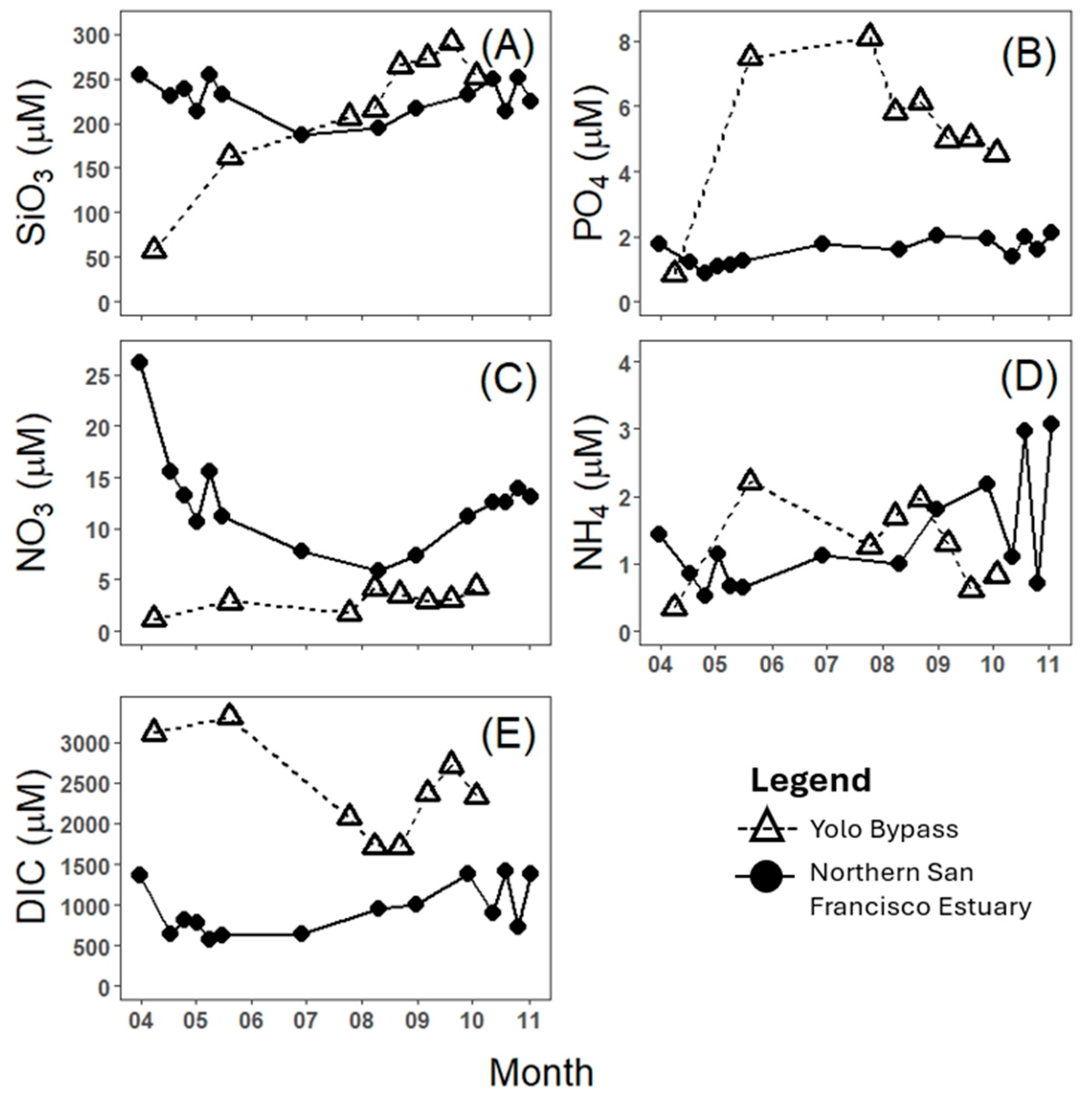
The YB and nSFE regions (Figure 1) showed different trends in nutrients and DIC during the study period. As regional averages, silicate (SiO3) was abundant (>>150 µM) throughout the study, with the lowest concentration appearing on the first sampling date in the YB (8 April), where the average SiO3 was 60 µM (Figure 2A). Phosphate (PO4) was relatively constant in the nSFE throughout the study (<1–2 µM) and more variable in the YB, where average PO4 was ~1 µM in April and rose to 8 µM in the summer before falling to 5–6 µM in the fall (Figure 2B). Regional averages of nitrate (NO3) were relatively low in the YB throughout the study (<5 µM) and more variable in the nSFE, where NO3 was >25 µM in the early spring and <10 µM in the summer (Figure 2C). Ammonium (NH4) was variable throughout the year in both the YB and nSFE; however, averaged regional values remained below 3 µM (Figure 2D). The concentrations of dissolved inorganic carbon (DIC) were between 2 and 6 times higher in the YB (1700–3200 µM) than in the nSFE (<500–1300 µM) (Figure 2E).
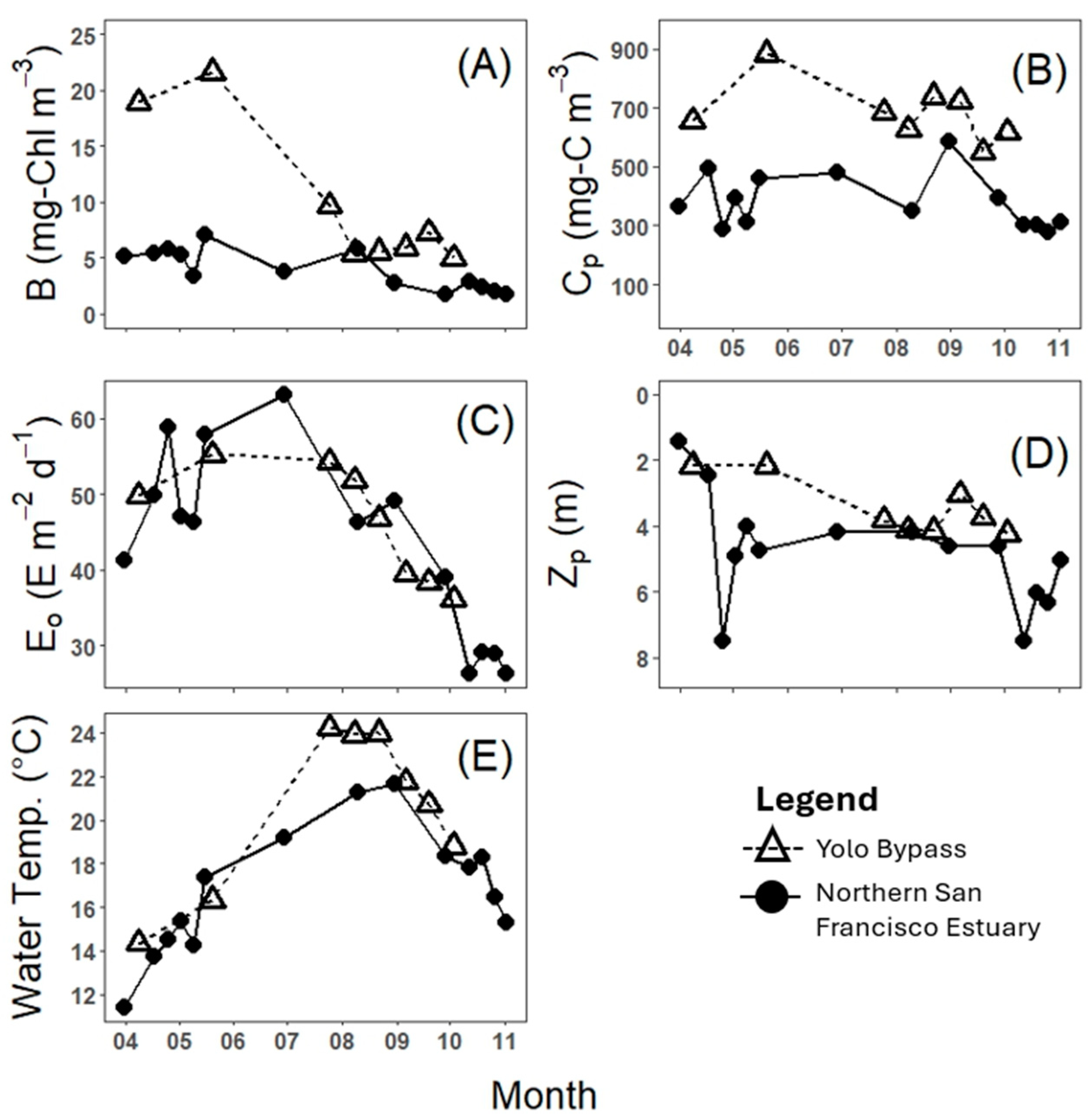
Regionally averaged phytoplankton biomass, B, was relatively high in April and May in the YB (~20 mg-Chl m−3) and decreased to ~6 mg-Chl m−3 in the summer and fall months (Figure 3A). The elevated B in the spring may have been driven by a diatom bloom as the increase in B was accompanied by a decline in SiO3, PO4, and NO3 (Figure 2A–C). Limited visualization of the phytoplankton community using a FlowCam qualitatively revealed that much of this B was composed of pennate diatoms. B in the nSFE was variable throughout the year, reaching a peak in May (~7 mg-Chl m−3) and a low in the fall (~1 mg-Chl m−3). Regionally averaged Cp was variable throughout the year but was consistently higher in the YB (~560–870 mg-C m−3) than in the nSFE (~260–570 mg-C m−3) throughout the year (Figure 3B). In both the YB and the nSFE, as expected, Eo (daily PAR) primarily decreased as a function of the number of Julian days away from the summer solstice (June 21st), although cloudy or foggy weather interrupted this signal in the nSFE (e.g., May and August in Figure 3C). Zp was shallow in the spring (<1 m) and deepened to ~3.5–4 m by the fall in the YB (Figure 3D). Sharp fluctuations in Zp occurred in nSFE during the spring (between <1 m and ~7 m) and fall (~4 m and ~7 m) but Zp was less variable in the summer (~4–5 m). Water temperature increased in both regions between March (~12–14 °C) and August (~21–24 °C) and then decreased into October and November (~16–19 °C) (Figure 3E).
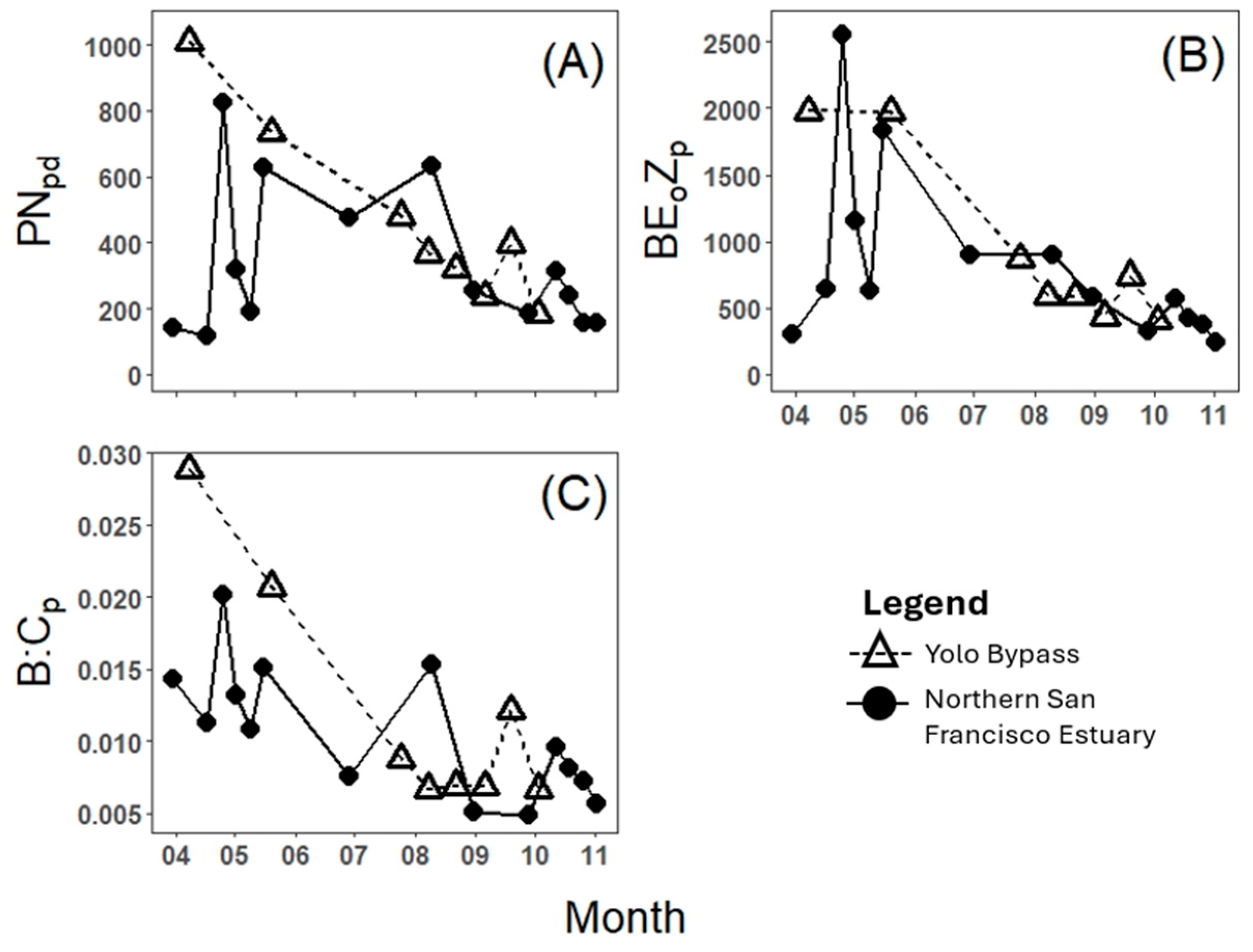
Depth-integrated daily primary productivity, PNpd, decreased gradually over the year in the YB, ranging from 1000 mg-C m−2 d−1 in April to 250 mg-C m−2 d−1 in October (Figure 4A). PNpd was more variable over the year in the nSFE, ranging between <200 and ~820 mg-C m−2 d−1 (Figure 4A). Overall, PNpy for 2023 was 137 ± 24 g-C m−2 yr−1 (Table 2). Estimating PNpy by integrating monthly averages of PNpd over a full year and filling in missing winter months with the smallest monthly average resulted in 111 ± 54 g-C m−2 yr−1. This approach is not significantly different from the approach in Equation (4); therefore, it was not repeated for the models. The composite parameter used in the LUM, BE0Zp, ranged between 250 and 2500 E mg-Chl m−4 d−1 (Figure 4B) and that used in the CCM, B:Cp, ranged between 5 × 10⁻³ and 3 × 10⁻² mg-Chl mg-C−1 (Figure 4C).
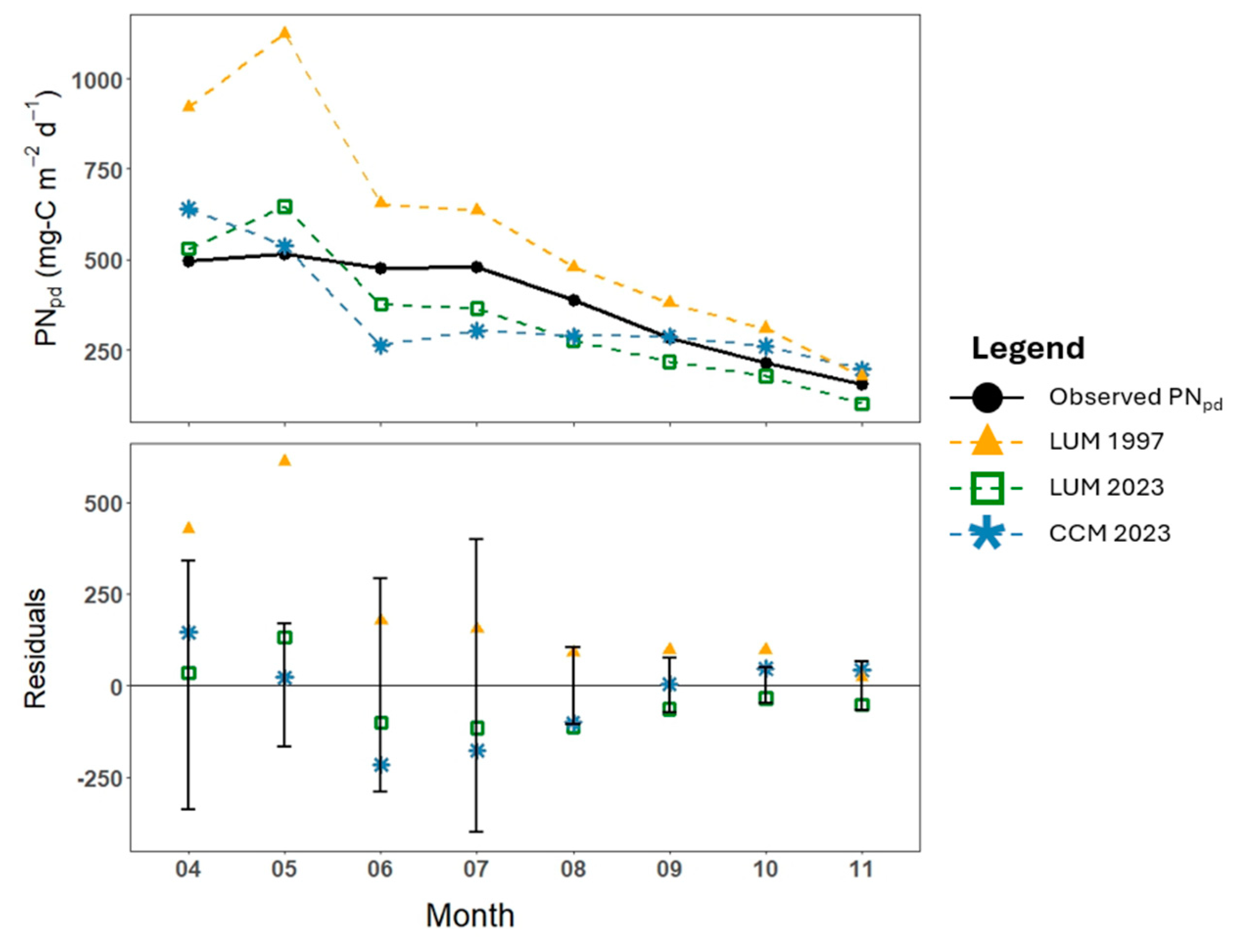
There were strong linear relationships between BE0Zp and measured PNpd (r2 = 0.89, p < 0.001, n = 76) and between B:Cp and measured PNpd (r2 = 0.85, p < 0.001, n = 76) (Figure 5A,B). The linear regression between BE0Zp and measured PNpd in this study (i.e., LUM 2023) resulted in ψ = 0.42 (Figure 5A). Based on the MAE, estimates of PNpd—produced using the product of ψ = 0.42 and measured BE0Zp from this study—are accompanied with 31% uncertainty (Table 2). Using ψ = 0.42 to estimate monthly averages of PNpd produces overestimates of measured PNpd for April and May and underestimates for the remainder of the months in the year (Figure 6). Overall, the estimate of PNpy produced using ψ = 0.42 was 125 g-C m−2 yr−1, or a 9% underestimate of measured PNpy (Table 2). All but one monthly average PNpd estimate (August) and the PNpy estimate fell within the observed CI95 (Figure 6 and Table 2). Finally, the linear regression between B:Cp and measured PNpd resulted in Ω = 3.47× 10⁴ (i.e., CCM 2023) (Figure 5B) and is accompanied with 36% uncertainty according to the MAE (Table 2). PNpy estimated using Ω = 3.47 × 10⁴ is 131 g-C m−2 yr−1, which is 4% smaller than the observed PNpy. All monthly average PNpd estimates produced using Ω = 3.47 × 10⁴ fell within the observed CI95 (Figure 6), a fact that is also true of the PNpy estimate (Table 2).

4. Discussion

This study set out to directly measure net estuarine phytoplankton productivity (PNpd) using the stable isotope 13C tracer along with measures of phytoplankton biomass (B and Cp) and light availability (Eo and Zp), such that modeling approaches for net phytoplankton productivity could be compared. The results show that daily rates of PNpd and B were quite variable within and between distinct regions of the SFED throughout 2023 (Figure 3A and Figure 4A), even though Eo and Zp were relatively similar in pattern and magnitude. A comparison of estimated values of PNpd and PNpy produced from the LUM calibrated in this study and in prior studies [5] shows that the LUM is not reliable for estimating carbon uptake beyond the dataset it was calibrated with. In this study, applying an LUM calibrated in 1997 [5] to data collected in 2023 resulted in a 58% overestimate of PNpy, which did not fall within the CI95 of observed PNpy. A CCM approach was shown to be a successful alternative to the LUM approach for estimating PNpd and PNpy and could be run simultaneously to improve model validation and predictability.
Although 14C is more sensitive, the use of 13C was particularly advantageous for this study as it did not require strict safety protocols for using radioactive 14C in the field [34]. PNpy estimated in this study (137 ± 24 g-C m−2 yr−1) compares well with prior determinations in the SFED, which have ranged from 90 ± 13 g-C m−2 yr−1 in the Delta [5] to 120 g-C m−2 yr−1 in San Francisco Bay [10,35]. PNpy was also estimated by integrating monthly averages of PNpd over a full year, filling in missing winter months with the smallest monthly average measured. This approach yielded an estimate of PNpy that was smaller (111 ± 54 g-C m−2 yr−1) but not significantly different from the estimate produced from Equation (4). As such, the SFED continues to rank in the lower half of estuaries where PNpy has been measured [36]. The SFED also continues to straddle the line between an oligotrophic (<100 g-C m−2 yr−1) and mesotrophic estuary (100–300 g-C m−2 yr−1) as defined in Nixon [37], even though there are abundant nutrients (Figure 2). As such, the SFED can continue to be described as a high-nutrient, low-chlorophyll (growth) estuary [38,39,40].
A leading explanation for why the SFED classifies as an oligo-mesotrophic estuary, despite substantial nutrient loading, is that phytoplankton are chronically light-limited [5,10]. The Dutch Scheldt Estuary is another example of this phenomenon [41] in addition to the Bristol Channel, U.K. [42], Roskeeda Bay, U.K. [43], and the Colne Estuary, U.K. [44]. It is indisputable that phytoplankton require light energy to fix ambient inorganic carbon and that these are in some way proportional. As such, the LUM approach for modeling PNpd using ψ is well iterated in estuarine systems, none more than the SFED (e.g., [5,10,12,35,45,46]). For datasets limited to ~1–2 years, the LUM estimates PNpd well, based on a single calibration of ψ [10,47]. However, when a single ψ is applied to longer duration datasets, the predictive potential of the LUM is considerably reduced—an issue all phytoplankton productivity models suffer from [15,48,49]. This ‘long dataset’ issue is made particularly evident for the LUM when studies determining ψ in different years are compiled [12] (Table 3). Each study determining ψ in the SFED, including this study, shows that ψ varies interannually and has generally decreased since the turn of the millennium (Table 3), confirming recent conclusions about the general use of the LUM in estuaries [12]. Some of the differences in values of ψ are certainly due to methodological differences (e.g., incubation length, the isotopic tracer used, and instrumentation), though much of the differences must also be due to limitations of the model [50]. Additionally, the implications of differences in methodology have been discussed previously and are mostly thought to be inconsequential [5,8,12].
For 2023, ψ was determined to be 0.42 ± 0.02—a significant deviation from all prior determinations save one study in the Central SF Bay [46] (Table 3). The LUM and ψ for this study (referred to as LUM 2023) are highlighted by a strong linear relationship (r2 = 0.89, p < 0.001) between PNpd and BEoZp but come with a large CI95 for estimates (319 mg-C m−2 d−1) (Figure 5). CI95 were not reported in prior studies. The PNpy estimate using LUM 2023 fell within the observed CI95 and is overall a 9% underestimate of measured PNpy. Furthermore, as a model, LUM 2023 is ~31% uncertain based on the MAE (Table 2).
To emphasize the ‘long dataset’ issue discussed earlier, a commonly used value of ψ (0.73) in the SFED [5] was applied to BEoZp collected in this study (referred to as LUM 1997) to assess its retrieval of measured PNpd (Figure 6). Monthly averaged PNpd estimates derived from LUM 1997 are consistent overestimates of measured PNpd. Notably, during spring months (April and May) when a putative diatom bloom occurred in the YB (see Figure 2A–C and Figure 3A), monthly averaged PNpd estimates from LUM 1997 fell outside of the observed CI95. The PNpy estimate from LUM 1997 also fell outside of the observed CI95 and, overall, there was a 58% overestimate accompanied by 61% uncertainty (Table 2). We can, therefore, echo conclusions that the LUM model is not fit for general use on long estuarine timeseries [12,15]—at least as a solitary approach. In this study, determinations of ψ were also significantly different for the nSFE and YB regions, a finding similar to those in the Scheldt Estuary, where ψ varied greatly station to station [16]. For the Scheldt estuary, this was partly due to the variability in Zp over a tidal cycle; however, other explanations may be related to differences in residence time between the nSFE and YB in this study as well [51].
The CCM performed here between B:Cp and PNpd (CCM 2023) had a strong linear relationship (r2 = 0.85, p < 0.001) and CI95 (366 mg-C m−2 d−1) and uncertainty (36%) that were similar to values seen for LUM 2023 (Figure 6). Overall, monthly averaged PNpd and the annual PNpy estimate (131 g-C m−1 yr−1) from CCM 2023 all fell within the observed CI95 (Figure 6 and Table 2). In comparing the CCM and LUM, these results suggest that neither is better than the other. Specifically, the LUM had superior model statistics (i.e., r2 and CI95 width); however, the CCM produced a more precise annual estimate (4% vs. 9% underestimate). Thus, these models performed similarly, produced agreeable results, and could be used together prospectively—or retrospectively—to validate PNpd estimates in estuarine systems. Still, it continues to be important to recognize the limitations of these simplistic models that arise from underlying assumptions. For example, the assumption in this study that a fixed proportion of POC was phytoplanktonic is complicated by the potential variability of detrital matter that was not assessed. Additionally, the assumption that ambient PAR and photic zone depths are the absolute measures to assess light availability to phytoplankton denies the consideration of how rates of vertical mixing affect access to the photic zone and what the physiological readiness of phytoplankton to utilize available light is. Finally, this study has shown that it is a poor assumption to consider the values of ψ and Ω to be constants and that the utilization of both the LUM and CCM require occasional recalibration to assess variability in these models. As such, these models and underlying assumptions could be better tested together in estuaries by utilizing pre-existing continuous monitoring networks, like the one present in the SFED to complement discrete studies such as this one. This could be accomplished by leveraging optical instrumentation that is or can be installed on pilings and piers to measure chlorophyll-a fluorescence and turbidity (EXO2 sondes), ambient PAR (LI COR sensors), and estimate Cp (e.g., WET Labs ECO-BB3 [17]). For estimating Cp from optical instrumentation, special care would need to be taken to consider different ambient conditions in estuaries, since previous applications were conducted in oceanic settings mostly free of detrital carbon [17,52].
On their own, simple linear models, such as the LUM and CCM, fail to capture the reality of stochastic fluid systems—something estuaries exemplify. In its a priori, the LUM does not consider the many abiotic and biotic factors (initial conditions) driving PNpd that may be significantly different over small or large timescales [10]. The CCM begins to inherently incorporate other factors, like nutrient conditions [18 and references therein], into its estimation of PNpd. For example, in a scenario where there was a temporal or regional change to nutrient loading, such that a limiting nutrient emerged, estimations of ψ from the LUM would not necessarily capture this effect on productivity, leading to variability in ψ, whereas estimations of Ω from the CCM would likely capture this effect, leading to more consistency in Ω. By pairing simple linear models that capture a wider range of initial conditions, we can cross-examine and validate results and predict reality with more confidence. The simultaneous application of multiple models is a common practice in forecasting natural scenarios [53]. The same practice can be applied to modeling PNpd, where using an ensemble of simplistic models would improve our confidence in outputs. By packaging simplistic models together, we can assess model agreement, identify patterns of cases where models disagree, and investigate the roots of these disagreements.

5. Conclusions

Here, we suggest a simple approach of packaging the LUM with a CCM for future efforts with an aim to model PNpd. The choice to complement the LUM with a CCM is based on success with CCMs in oceanography [28], correlative behavior observed between B:Cp, the growth rate µ, and net phytoplankton productivity [17,18] and because B:Cp is simple to measure alongside the LUM methodology and can be measured simply using shipboard sensors or satellites [17,28,54]. The results of this research show that (1) the SFED continues to be an oligo-mesotrophic estuary despite nutrient loading, (2) the ‘long dataset’ issue persists with the LUM approach to modeling PNpd, reinforcing the importance of periodic recalibration, and (3) we demonstrate how expanding the toolbox available for modeling may lead to more precise estimates of net phytoplankton productivity through an ensemble modeling approach.

Author Contributions

Conceptualization, R.H., F.W. and A.P.; methodology, R.H., F.W., R.D. and A.P.; formal analysis, R.H.; investigation, R.H.; data curation, R.H.; writing—original draft preparation, R.H.; writing—review and editing, R.H., F.W. and A.P.; project administration, F.W.; funding acquisition, R.D. and F.W. All authors have read and agreed to the published version of the manuscript.

Funding

This work was supported through Proposition 1 with the California Department of Fish and Wildlife under agreement numbers Q1996035 and Q2196008 with Dr. Dugdale, the State Water Contractors under agreement number 20–43 with Dr. Wilkerson, the Department of Water Resources under contract 4600013243 with Dr. Dugdale, and the 2023 Maxwell/Hanrahan Scientific Illustration Grant.

Data Availability Statement

Data are being deposited in the Environmental Data Initiative (EDI) https://environmentaldatainitiative.org/, accessed on 5 October 2024.

Acknowledgments

We thank S. Blaser, B. Gustafson, S. Randall, A. Chu (Estuary and Ocean Science Center, San Francisco State University) and E. Jones, D. Terrusa (California State University Maritime Academy), and CA DWR staff for participation in sample collection on cruises and lab analyses, as well as Captain N. Shields of the R/V Questuary at the Golden Bear Research Center, CSU Maritime Academy.

Conflicts of Interest

The authors declare no conflicts of interest. The funders had no role in the design of the study; in the collection, analyses, or interpretation of data; in the writing of the manuscript; or in the decision to publish the results.

References

  1. Davidson, N.C. How much wetland has the world lost? Long-term and recent trends in global wetland area. Mar. Freshw. Res. 2014, 65, 934. [Google Scholar] [CrossRef]
  2. Milligan, B.; Kraus-Polk, A. Evolving the Evolving: Territory, Place and Rewilding in the California Delta. Urban Plan. 2017, 2, 93–114. [Google Scholar] [CrossRef]
  3. Cloern, J.E.; Safran, S.M.; Smith Vaughn, L.; Robinson, A.; Whipple, A.A.; Boyer, K.E.; Drexler, J.Z.; Naiman, R.J.; Pinckney, J.L.; Howe, E.R.; et al. On the human appropriation of wetland primary production. Sci. Total Environ. 2021, 785, 147097. [Google Scholar] [CrossRef]
  4. Sommer, T.; Armor, C.; Baxter, R.; Breuer, R.; Brown, L.; Chotkowski, M.; Culberson, S.; Feyrer, F.; Gingras, M.; Herbold, B.; et al. The Collapse of Pelagic Fishes in the Upper San Francisco Estuary. Fisheries 2007, 32, 270–277. [Google Scholar] [CrossRef]
  5. Jassby, A.; Cloern, J.; Cole, B. Annual primary production: Patterns and mechanisms of change in a nutrient-rich tidal ecosystem. Limnol. Oceanogr. 2002, 47, 698–712. [Google Scholar] [CrossRef]
  6. Gross, E.; Holleman, R.; Kimmerer, W.; Munger, S.; Burdick, S.; Durand, J. Using Age Tracers to Estimate Ecological Rates in a Phytoplankton Model. Water 2023, 15, 2097. [Google Scholar] [CrossRef]
  7. Cloern, J. Tidal stirring and phytoplankton bloom dynamics in an estuary. J. Mar. Res. 1991, 49, 203–221. [Google Scholar] [CrossRef]
  8. Slawyk, G.; Collos, Y.; Auclair, J. The use of the 13C and 15N isotopes for the simultaneous measurement of carbon and nitrogen turnover rates in marine phytoplankton. Limnol. Oceanogr. 1977, 22, 925–932. [Google Scholar] [CrossRef]
  9. Dugdale, R.C.; Wilkerson, F.P. The use of 15N to measure nitrogen uptake in eutrophic oceans; experimental considerations. Limnol. Oceanogr. 1986, 31, 673–689. [Google Scholar] [CrossRef]
  10. Cole, B.; Cloern, J. Significance of biomass and light availability to phytoplankton productiivty in San Francisco Bay. Mar. Ecol. Prog. Ser. 1984, 17, 15–24. [Google Scholar] [CrossRef]
  11. Kimmerer, W.; Parker, A.; Lidström, U.; Carpenter, E. Short-Term and Interannual Variability in Primary Production in the Low-Salinity Zone of the San Francisco Estuary. Estuaries Coasts 2012, 35, 913–929. [Google Scholar] [CrossRef]
  12. Parker, A.; Kimmerer, W.; Lidström, U. Reevaluating the Generality of an Empirical Model for Light-Limited Primary Production in the San Francisco Estuary. Estuaries Coasts 2012, 35, 930–942. [Google Scholar] [CrossRef]
  13. Jassby, A. Phytoplankton in the Upper San Francisco Estuary: Recent Biomass Trends, Their Causes, and Their Trophic Significance. San Franc. Estuary Watershed Sci. 2008, 6. [Google Scholar] [CrossRef]
  14. Cloern, J.E.; Jassby, A.D.; Thompson, J.K.; Hieb, K.A. A cold phase of the East Pacific triggers new phytoplankton blooms in San Francisco Bay. Proc. Natl. Acad. Sci. USA 2007, 104, 18561–18565. [Google Scholar] [CrossRef] [PubMed]
  15. Harding, L.W.; Mallonee, M.E.; Perry, E.S. Toward a Predictive Understanding of Primary Productivity in a Temperate, Partially Stratified Estuary. Estuar. Coast. Shelf Sci. 2002, 55, 437–463. [Google Scholar] [CrossRef]
  16. Kromkamp, J.; Peene, J.; Van Rijswijk, P.; Sandee, A.; Goosen, N. Nutrients, light and primary production by phytoplankton and microphytobenthos in the eutrophic, turbid Westerschelde estuary (The Netherlands). Hydrobiologia 1995, 311, 9–19. [Google Scholar] [CrossRef]
  17. Burt, W.J.; Westberry, T.K.; Behrenfeld, M.J.; Zeng, C.; Izett, R.W.; Tortell, P.D. Carbon: Chlorophyll Ratios and Net Primary Productivity of Subarctic Pacific Surface Waters Derived From Autonomous Shipboard Sensors. Glob. Biogeochem. Cycles 2018, 32, 267–288. [Google Scholar] [CrossRef]
  18. Cloern, J.E.; Grenz, C.; Vidergar-Lucas, L. An empirical model of the phytoplankton chlorophyll: Carbon ratio—The conversion factor between productivity and growth rate. Limnol. Oceanogr. 1995, 40, 1313–1321. [Google Scholar] [CrossRef]
  19. Parker, A.; Fuller, J.; Dugdale, R. Estimating dissolved inorganic carbon concentrations from salinity in San Francisco Bay for use in 14C-primary production studies. Interag. Ecol. Program San Franc. Estuary 2006, 19, 17–22. [Google Scholar]
  20. Arar, E.; Collins, G. Method 445.0: In Vitro Determination of Chlorophyll a and Pheophytin a in Marine and Freshwater Algae by Fluorescence; National Exposure Research Laboratory, Office of Research and Development, U.S. Environmental Protection Agency: Cincinnati, OH, USA, 1997.
  21. Solórzano, L. Determination of Ammonia in Natural Waters by the Phenolhypochlorite Method. Limnol. Oceanogr. 1969, 14, 799–801. [Google Scholar] [CrossRef]
  22. Bran Luebbe Inc. Bran Luebbe Autoanalyzer Applications: Autoanalyzer Method No. G-177-96 Silicate in Water and Seawater; Bran Luebbe Inc.: Buffalo Grove, IL, USA, 1999. [Google Scholar]
  23. Bran Luebbe Inc. Bran Luebbe Autoanalyzer Applications: Autoanalyzer Method No. G-175-96 Phosphate in Water and Seawater; Bran Luebbe Inc.: Buffalo Grove, IL, USA, 1999. [Google Scholar]
  24. Bran Luebbe Inc. Bran Luebbe Autoanalyzer Applications: Autoanalyzer Method No. G-172-96 Nitrate and Nitrite in Water and Seawater; Bran Luebbe Inc.: Buffalo Grove, IL, USA, 1999. [Google Scholar]
  25. Wilkerson, F.; Dugdale, R.; Parker, A.; Blaser, S.; Pimenta, A. Nutrient uptake and primary productivity in an urban estuary: Using rate measurements to evaluate phytoplankton response to different hydrological and nutrient conditions. Aquat. Ecol. 2015, 49, 211–233. [Google Scholar] [CrossRef]
  26. Parker, A.E. Differential supply of autochthonous organic carbon and nitrogen to the microbial loop in the Delaware Estuary. Estuaries 2005, 28, 856–867. [Google Scholar] [CrossRef]
  27. Legendre, L.; Gosselin, M. Estimation of N or C uptake rates by phytoplankton using 15N or 13C: Revisiting the usual computation formulae. J. Plankton Res. 1997, 19, 263–271. [Google Scholar] [CrossRef]
  28. Behrenfeld, M.J.; Boss, E.; Siegel, D.A.; Shea, D.M. Carbon-based ocean productivity and phytoplankton physiology from space. Glob. Biogeochem. Cycles 2005, 19, GB1006. [Google Scholar] [CrossRef]
  29. Jakobsen, H.H.; Markager, S. Carbon-to-chlorophyll ratio for phytoplankton in temperate coastal waters: Seasonal patterns and relationship to nutrients: C:Chl for phytoplankton in temperate coastal waters. Limnol. Oceanogr. 2016, 61, 1853–1868. [Google Scholar] [CrossRef]
  30. Franklin, J. Plant Growth Chamber Handbook. New Phytol. 1998, 138, 743–750. [Google Scholar] [CrossRef]
  31. Zeileis, A.; Hothorn, T. Diagnostic Checking in Regression Relationships. R News 2002, 2, 7–10. [Google Scholar]
  32. R Core Team R: A Language and Environment for Statistical Computing; R Foundation for Statistical Computing: Vienna, Austria, 2024.
  33. Willmott, C.; Matsuura, K. Advantages of the mean absolute error (MAE) over the root mean square error (RMSE) in assessing average model performance. Clim. Res. 2005, 30, 79–82. [Google Scholar] [CrossRef]
  34. López-Sandoval, D.C.; Delgado-Huertas, A.; Agustí, S. The 13C method as a robust alternative to 14C-based measurements of primary productivity in the Mediterranean Sea. J. Plankton Res. 2018, 40, 544–554. [Google Scholar] [CrossRef]
  35. Cole, B.; Cloern, J. An empirical model for estimating phytoplankton productivity in estuaries. Mar. Ecol. Prog. Ser. 1987, 35, 299–305. [Google Scholar] [CrossRef]
  36. Cloern, J.E.; Foster, S.Q.; Kleckner, A.E. Phytoplankton primary production in the world’s estuarine-coastal ecosystems. Biogeosciences 2014, 11, 2477–2501. [Google Scholar] [CrossRef]
  37. Nixon, S.W. Coastal marine eutrophication: A definition, social causes, and future concerns. Ophelia 1995, 41, 199–219. [Google Scholar] [CrossRef]
  38. Cloern, J. Our evolving conceptual model of the coastal eutrophication problem. Mar. Ecol. Prog. Ser. 2001, 210, 223–253. [Google Scholar] [CrossRef]
  39. Sharp, J.H. Marine and Aquatic Communities, Stress from Eutrophication. In Encyclopedia of Biodiversity; Elsevier: Amsterdam, The Netherlands, 2001; pp. 1–11. ISBN 978-0-12-226865-6. [Google Scholar]
  40. Wilkerson, F.P.; Dugdale, R.C.; Hogue, V.E.; Marchi, A. Phytoplankton blooms and nitrogen productivity in San Francisco Bay. Estuaries Coasts 2006, 29, 401–416. [Google Scholar] [CrossRef]
  41. Gazeau, F.; Gattuso, J.-P.; Middelburg, J.J.; Brion, N.; Schiettecatte, L.-S.; Frankignoulle, M.; Borges, A.V. Planktonic and whole system metabolism in a nutrient-rich estuary (the Scheldt estuary). Estuaries 2005, 28, 868–883. [Google Scholar] [CrossRef]
  42. Joint, I.R.; Pomroy, A.J. Primary production in a turbid estuary. Estuar. Coast. Shelf Sci. 1981, 13, 303–316. [Google Scholar] [CrossRef]
  43. Raine, R.C.T.; Patching, J.W. Aspects of carbon and nitrogen cycling in a shallow marine environment. J. Exp. Mar. Biol. Ecol. 1980, 47, 127–139. [Google Scholar] [CrossRef]
  44. Kocum, E.; Underwood, G.; Nedwell, D. Simultaneous measurement of phytoplanktonic primary production, nutrient and light availability along a turbid, eutrophic UK east coast estuary (the Colne Estuary). Mar. Ecol. Prog. Ser. 2002, 231, 1–12. [Google Scholar] [CrossRef]
  45. Alpine, A.; Cloern, J. Trophic interactions and direct physical effects control phytoplankton biomass and production in an estuary. Limnol. Oceanogr. 1992, 37, 946–955. [Google Scholar] [CrossRef]
  46. Lorenzi, A. Primary Productivity and rbcL Gene Expression in Central San Francisco Bay; San Francisco State University: San Francisco, CA, USA, 2005. [Google Scholar]
  47. Harding, L.W.; Meeson, B.W.; Fisher, T.R. Phytoplankton production in two east coast estuaries: Photosynthesis-light functions and patterns of carbon assimilation in Chesapeake and Delaware Bays. Estuar. Coast. Shelf Sci. 1986, 23, 773–806. [Google Scholar] [CrossRef]
  48. Campbell, J.W.; O’Reilly, J.E. Role of satellites in estimating primary productivity on the northwest Atlantic continental shelf. Cont. Shelf Res. 1988, 8, 179–204. [Google Scholar] [CrossRef]
  49. Balch, W.; Evans, R.; Brown, J.; Feldman, G.; McClain, C.; Esaias, W. The remote sensing of ocean primary productivity: Use of a new data compilation to test satellite algorithms. J. Geophys. Res. Oceans 1992, 97, 2279–2293. [Google Scholar] [CrossRef]
  50. Behrenfeld, M.J.; Falkowski, P.G. Photosynthetic rates derived from satellite-based chlorophyll concentration. Limnol. Oceanogr. 1997, 42, 1–20. [Google Scholar] [CrossRef]
  51. Stumpner, E.B.; Bergamaschi, B.A.; Kraus, T.E.C.; Parker, A.E.; Wilkerson, F.P.; Downing, B.D.; Dugdale, R.C.; Murrell, M.C.; Carpenter, K.D.; Orlando, J.L.; et al. Spatial variability of phytoplankton in a shallow tidal freshwater system reveals complex controls on abundance and community structure. Sci. Total Environ. 2020, 700, 134392. [Google Scholar] [CrossRef] [PubMed]
  52. Graff, J.R.; Westberry, T.K.; Milligan, A.J.; Brown, M.B.; Dall’Olmo, G.; Dongen-Vogels, V.V.; Reifel, K.M.; Behrenfeld, M.J. Analytical phytoplankton carbon measurements spanning diverse ecosystems. Deep Sea Res. Part I Oceanogr. Res. Pap. 2015, 102, 16–25. [Google Scholar] [CrossRef]
  53. Gneiting, T.; Raftery, A.E. Weather Forecasting with Ensemble Methods. Science 2005, 310, 248–249. [Google Scholar] [CrossRef]
  54. Sathyendranath, S.; Stuart, V.; Nair, A.; Oka, K.; Nakane, T.; Bouman, H.; Forget, M.; Maass, H.; Platt, T. Carbon-to-chlorophyll ratio and growth rate of phytoplankton in the sea. Mar. Ecol. Prog. Ser. 2009, 383, 73–84. [Google Scholar] [CrossRef]
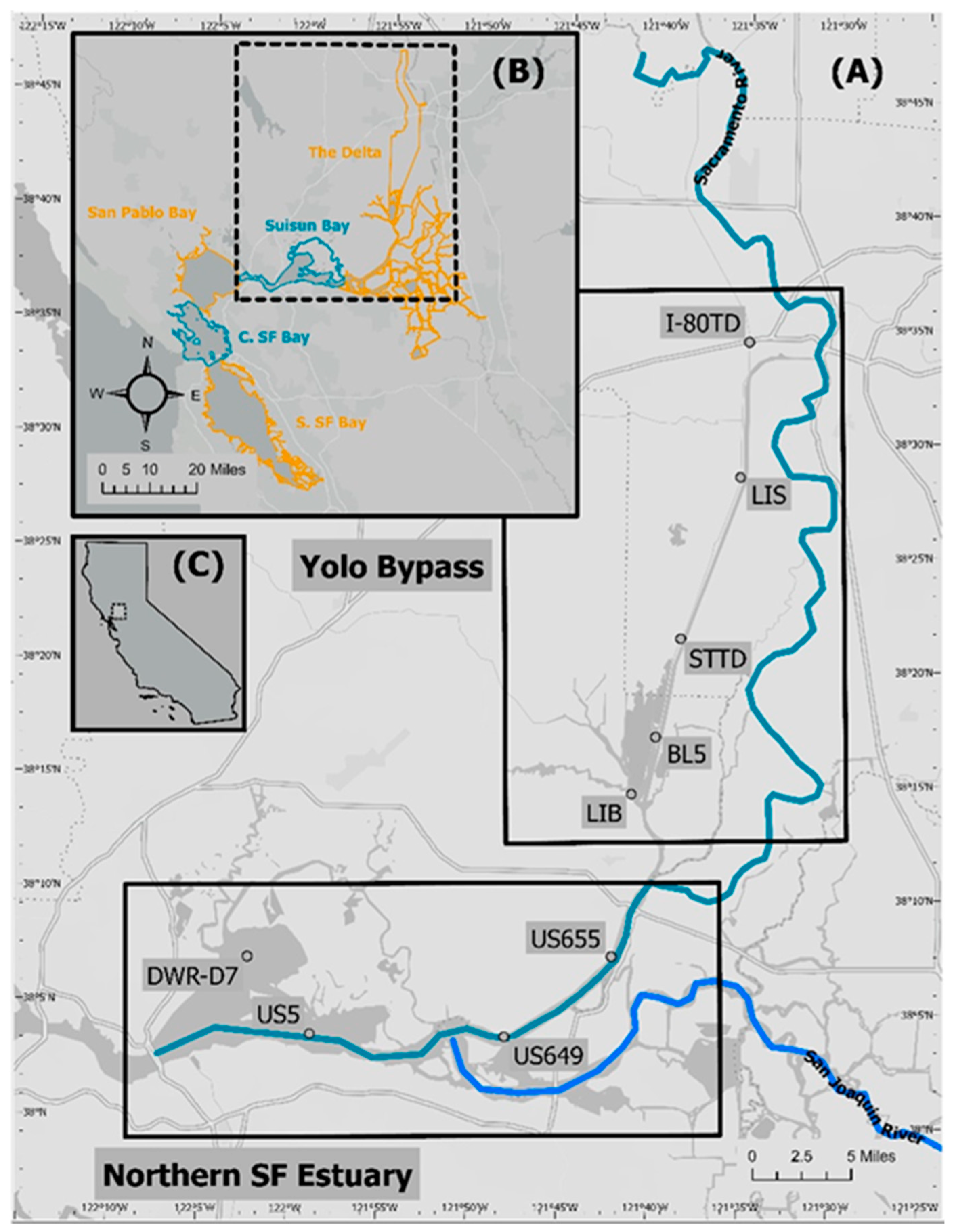
Figure 1. Map of the study region (A) showing the two main subregions, major rivers, and station locations where samples were collected. Large sub-embayments of the San Francisco Estuary and Delta are shown in subset map (B). The study region is shown in relation to the state of California, USA, in subset map (C).
Water 17 00747 g001
Figure 2. Regional averaged timeseries for the Yolo Bypass and the northern San Francisco Estuary versus month in 2023 of (A) silicate (SiO3), (B) phosphate (PO4), (C) nitrate (NO3), (D) ammonium (NH4), and (E) dissolved inorganic carbon (DIC) all in µM.
Water 17 00747 g002
Figure 3. Daily regional averages for the Yolo Bypass and the northern San Francisco Estuary versus month of (A) biomass, B in mg-Chl m−3, (B) Cp in mg-C m−3, (C) ambient photosynthetically active radiation (PAR), Eo as in E m−2 d−1, (D) photic zone depth, Zp in meters (note: reversed axis), and (E) water temperature in °C.
Water 17 00747 g003
Figure 4. Daily regional averages for the daily regional averages for the Yolo Bypass and the northern San Francisco Estuary of (A) primary productivity, PNpd in mg-C m−2 d−1, (B) composite parameter, BEoZp in E mg-Chl m−4 d−1, and (C) ratio B:Cp in units of mg-Chl (mg-C)−1.
Water 17 00747 g004
Figure 5. Results of the two modeling approaches, LUM (A) and CCM (B). Summary statistics are shown in the bottom right as text.
Water 17 00747 g005
Figure 6. Monthly averaged PNpd from observations made in 2023 in this study and model estimates versus month (top) using ψ reported in 1997 [5]—LUM1997, ψ from this study (Figure 5A)—LUM 2023, and Ω from this study (Figure 5B)—CCM 2023. Model residuals plotted against the CI95 error bars for each monthly average (bottom).
Water 17 00747 g006
Table 1. List of acronyms and symbols with units if applicable.
SymbolParameterUnits
SFEDSan Francisco Estuary and Delta
LUMlight utilization model
CCMchlorophyll-a to carbon model
ρCtransport (uptake) rate of carbonmg-C m−3 d−1
PNpddepth-integrated daily net phytoplankton productivitymg-C m−2 d−1
PNpydepth-integrated annual net phytoplankton productivityg-C m−2 yr−1
Bchlorophyll-a concentrationmg-Chl m−3
Eoambient photosynthetically active radiationEinsteins m−2 d−1
Zpphotic zone depthm
Cpphytoplankton carbon concentrationmg-C m−3
BEoZpcomposite parameterEinsteins mg-Chl m−4 d−1
B:Cpchlorophyll-a to phytoplankton carbon ratiomg-Chl mg-C−1
ψlight utilization model regression slopemg-C m2 mg-Chl−1 Einsteins−1
Ωchlorophyll-a to carbon model regression slopemgC2 mgChl−1 m−2 d−1
MAEmean absolute error
Table 2. Comparison of LUM and CCM model estimates for PNpy to observed values of PNpy from 13C incubations.
Estimate SourceRegression SlopePNpy Estimate
(g-C m−2 yr−1)
Within CI95MAEPercent Error
Observed-137±24--
LUM 2023Ψ = 0.42125Yes31%−9%
LUM 1997Ψ = 0.73217No61%58%
CCM 2023Ω = 3.47 × 104131Yes36%−4%
Table 3. Determination of the linear regression slope (ψ) reported here and refit or calculated from other published studies.
Year(s)Location(s)SeasonPhotoperiodψReference
2023nSFE + YBMarch–November24 h0.42 ± 0.02This study
nSFE data0.38 ± 0.02
YB data0.45 ± 0.02
1980South SF BayAnnual24 h0.99 ± 0.09[10] Cole & Cloern (1984),
refit data
San Pablo Bay data1.22 ± 0.15
1988Suisun BayMay–October24 h0.81 ± 0.10[45] Alpine & Cloern (1992), calculated from data in Table 2
1997DeltaMay–November30 m0.73 ± 0.05[5] Jassby et al. (2002),
as reported
2004–2005Central SF BayAnnual6 h0.37 ± 0.04[46] Lorenzi 2006, as reported
2006San Pablo—Suisun BayMarch–August6 h0.29 ± 0.03[12] Parker et al. (2012),
as reported
2007Suisun Bay 24 h0.56 ± 0.04
Disclaimer/Publisher’s Note: The statements, opinions and data contained in all publications are solely those of the individual author(s) and contributor(s) and not of MDPI and/or the editor(s). MDPI and/or the editor(s) disclaim responsibility for any injury to people or property resulting from any ideas, methods, instructions or products referred to in the content.