
Novel Numerical Modeling of a Groundwater Level-Lowering Approach Implemented in the Construction of High-Rise/Complex Buildings

 ,
, 
Abstract
1. Introduction
2. Materials and Methods
- Define the three-dimensional geometry of the geologic medium containing the groundwater;
- Identify the hydraulic properties of the materials through which the groundwater flow occurs;
- Specify boundary conditions congruent with the conceptual model of operation;
- Establish initial conditions of groundwater flow and hydraulic loads;
- Perform evaluations of the volumetric water flow term, which represents pumping extractions.
- Development of the conceptual model;
- Numerical model representation;
- Verification and calibration;
- Prediction and evaluation.
2.1. Development of Conceptual Model
- Definition of the geological and stratigraphy of the zone based on GIS data from the Instituto Nacional de Estadística y Geografía (INEGI), obtained through in situ geotechnical exploration;
- Topographic characterization using satellite imagery from INEGI with LiDAR digital models (5 m resolution), processed with QGIS (version 3.22) and Surfer 13 for a 3D model to integrate with the ModelMuse interface (version 4.1);
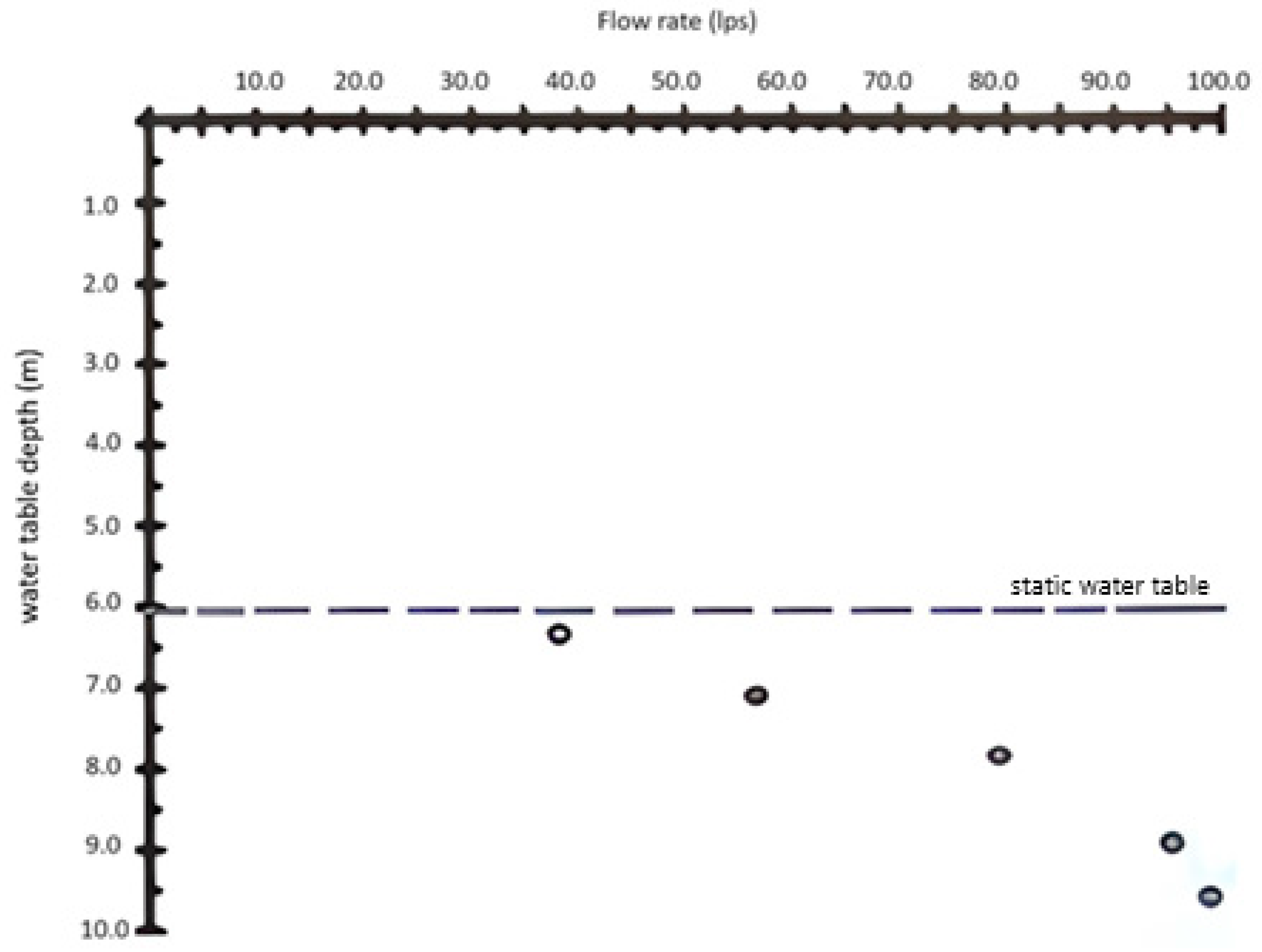
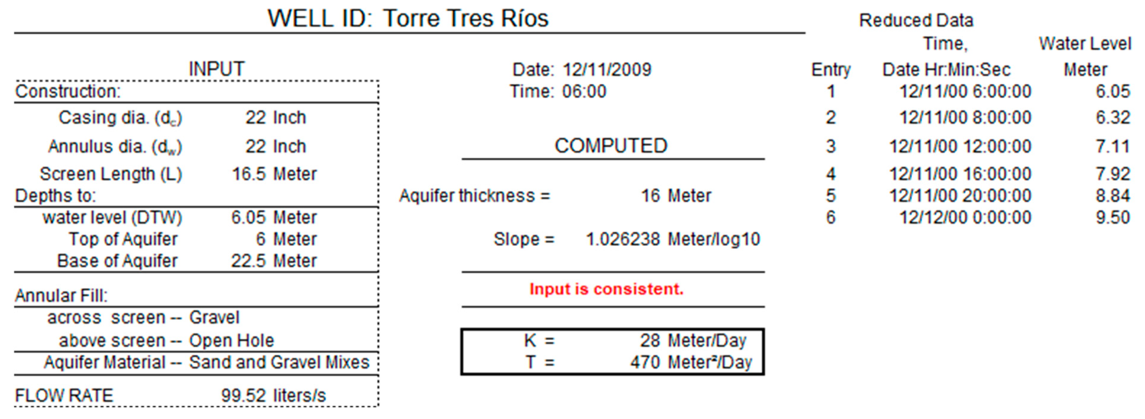
- Identification of hydraulic properties (hydraulic conductivity, transmissivity, and specific storage) of the aquifer using a pumping test and the Cooper–Jacob method, comparing the results with aquifer data from an available report [34];
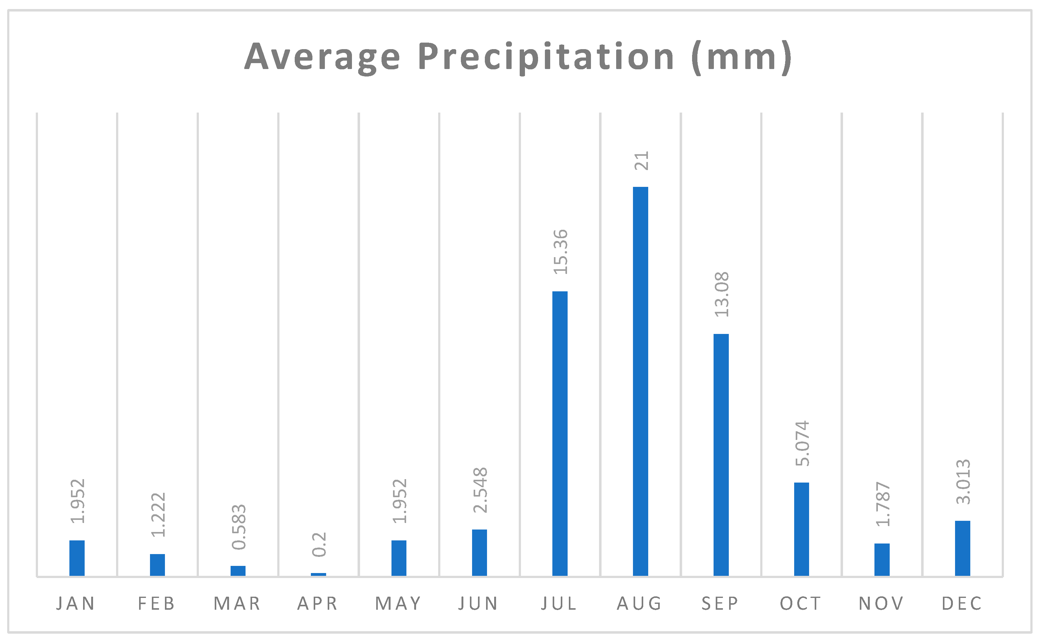
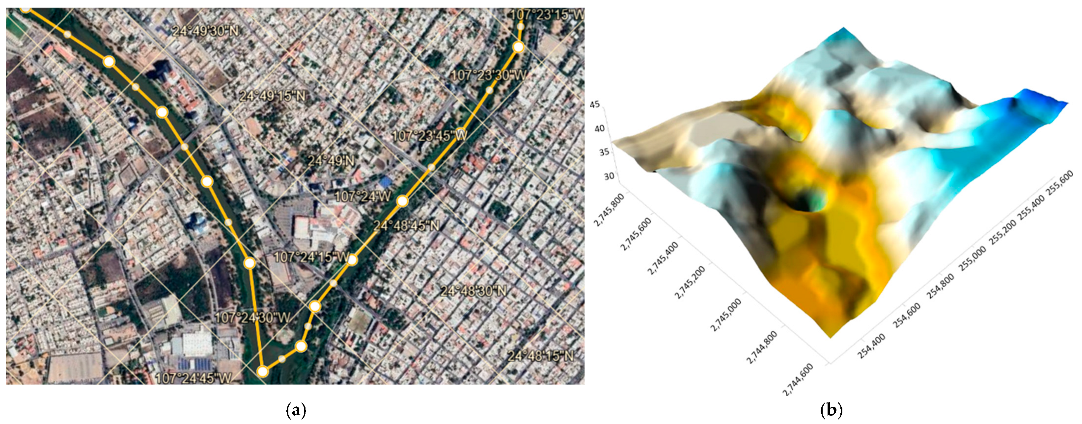
- Hydrologic and climatologic characterization conducted by analyzing recharge and discharge factors, including field measurements of the water table level with a Solinst 101 P7 level sensor (Solinst Canada Ltd.), data from local meteorological stations to assess precipitation’s influence, and hydrological data from Banco Nacional de Datos de Aguas Superficiales (BANDAS) from CONAGUA to consider the impact of the Humaya and Tamazula Rivers.
2.2. Development of Numerical Model
- Q: flow rate (m3/s);
- k: hydraulic conductivity (m/s);
- i: hydraulic gradient;
- A: cross-sectional area (m2).
- Ss: specific storage coefficient (1/m);
- ∂h/∂t: change in hydraulic head over time (m/s);
- ∇: divergence operator (1/m);
- ∇h: gradient of hydraulic head (m/m);
- K: hydraulic conductivity (m/s);
- W: volumetric flow rate per unit volume (1/s).
2.2.1. Spatial and Temporary Discretization
2.2.2. Steady and Transient States
- Constant load (Type I or Dirichlet’s) imposes the existence of piezometric heights or pre-described hydraulic potentials;
- Constant flow (Type II or Neumann) simulates a constant flow in the model, representing the main inputs and outputs of the system;
- Dependent load (Type III, Cauchy or Mixed) combines characteristics of the previous two, simulating interactions with other water bodies, like rivers.
- LMT (Layer-Property Flow) simulates flow in heterogeneous and anisotropic layers;
- RIV (River Package) models the exchange of water between rivers and aquifers;
- RCH (Recharge) simulates recharge (water input) to the aquifer from external sources like precipitation;
- WEL (Well) models water extraction from wells.
2.3. Calibration and Validation
- The mean absolute error (MAE);
- The standard deviation (SD).
- MAE = mean absolute error;
- SD = standard deviation;
- n = number of observations;
- hoi = observed hydraulic load (m);
- hi = calculated hydraulic load (m).
2.4. Sensitivity and Uncertainty Analysis Method
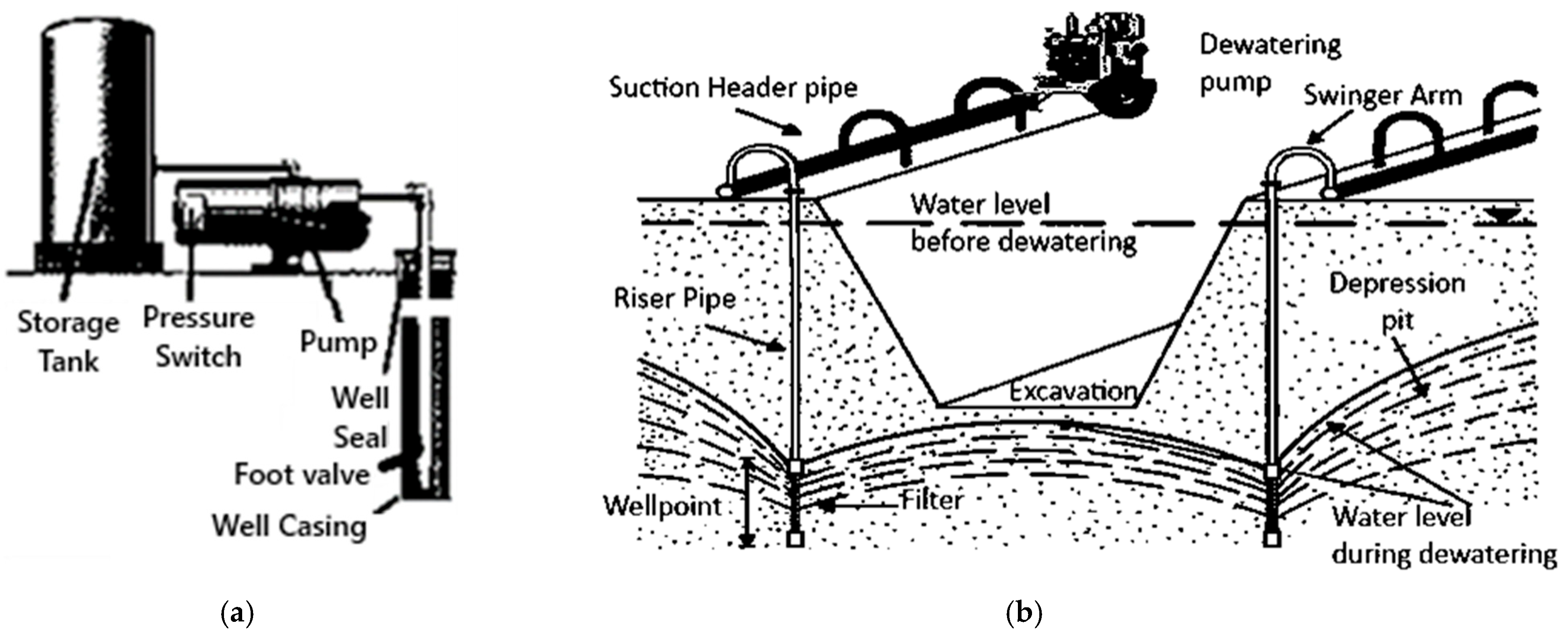
2.5. Dewatering System
- r = radius of influence (m);
- Q = pumping rate (m3/s);
- K = hydraulic conductivity (m/s);
- ∆h = drawdown (m).
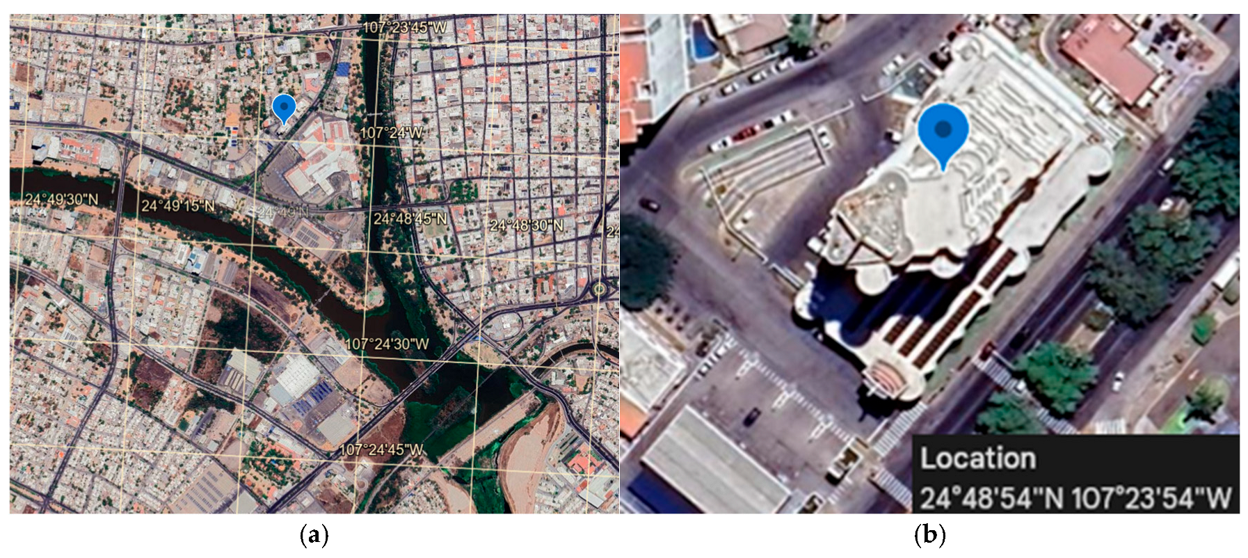
3. Case Study
3.1. Conceptual Hydrogeological Model
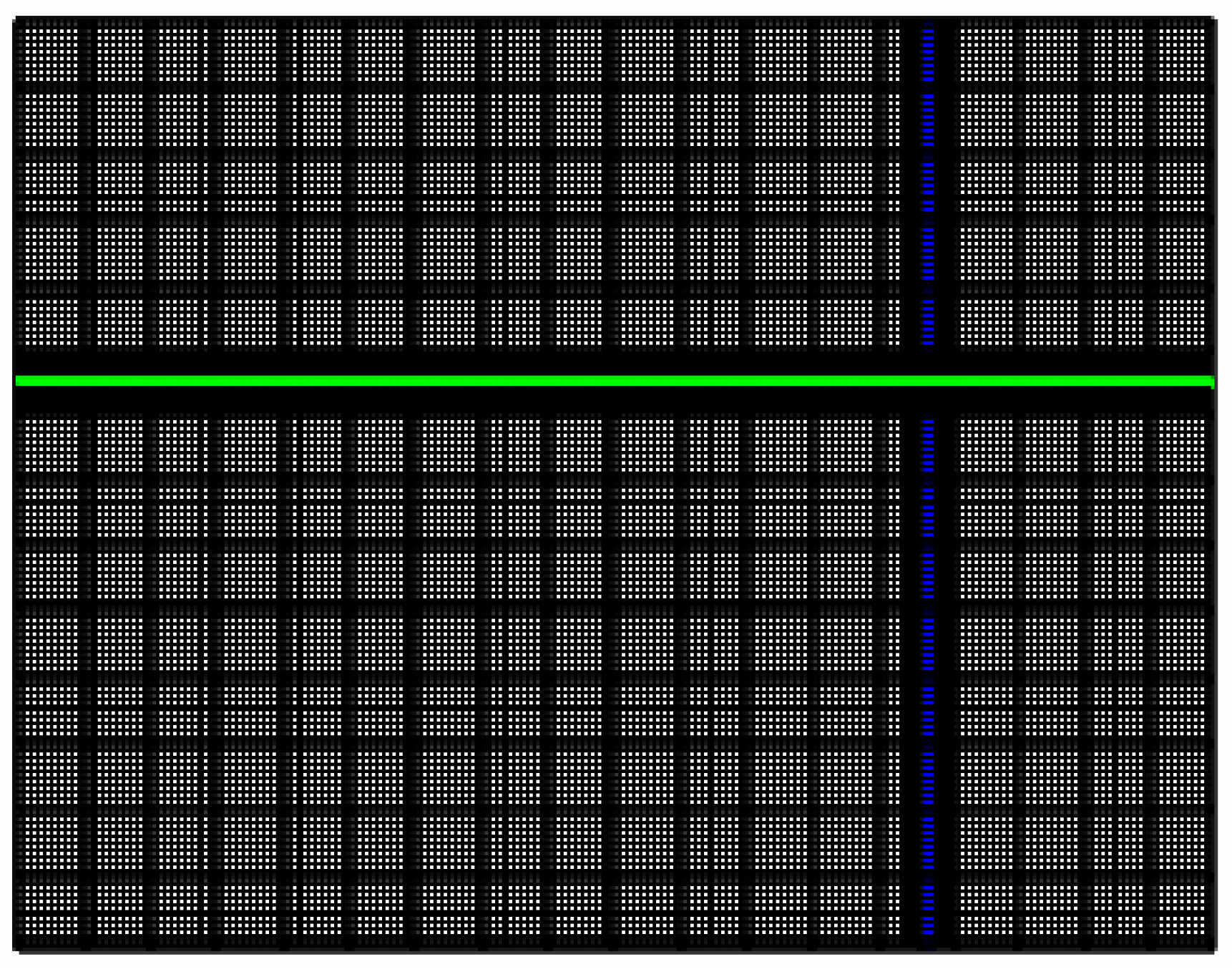
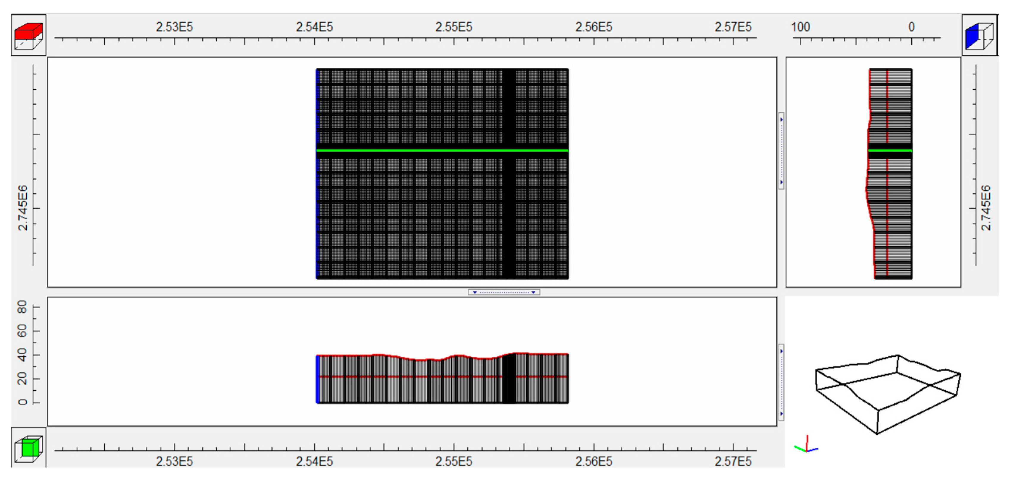
3.2. Numerical Model
3.2.1. Spatial and Temporary Discretization Model
3.2.2. Steady-State Flow Model
3.2.3. Transient-State Flow Model
3.2.4. Sensitivity and Uncertainty Analysis
3.3. Dewatering System Model
4. Results and Discussion
4.1. Calibration of the Model
4.2. Sensitivity and Uncertainty Analysis Results
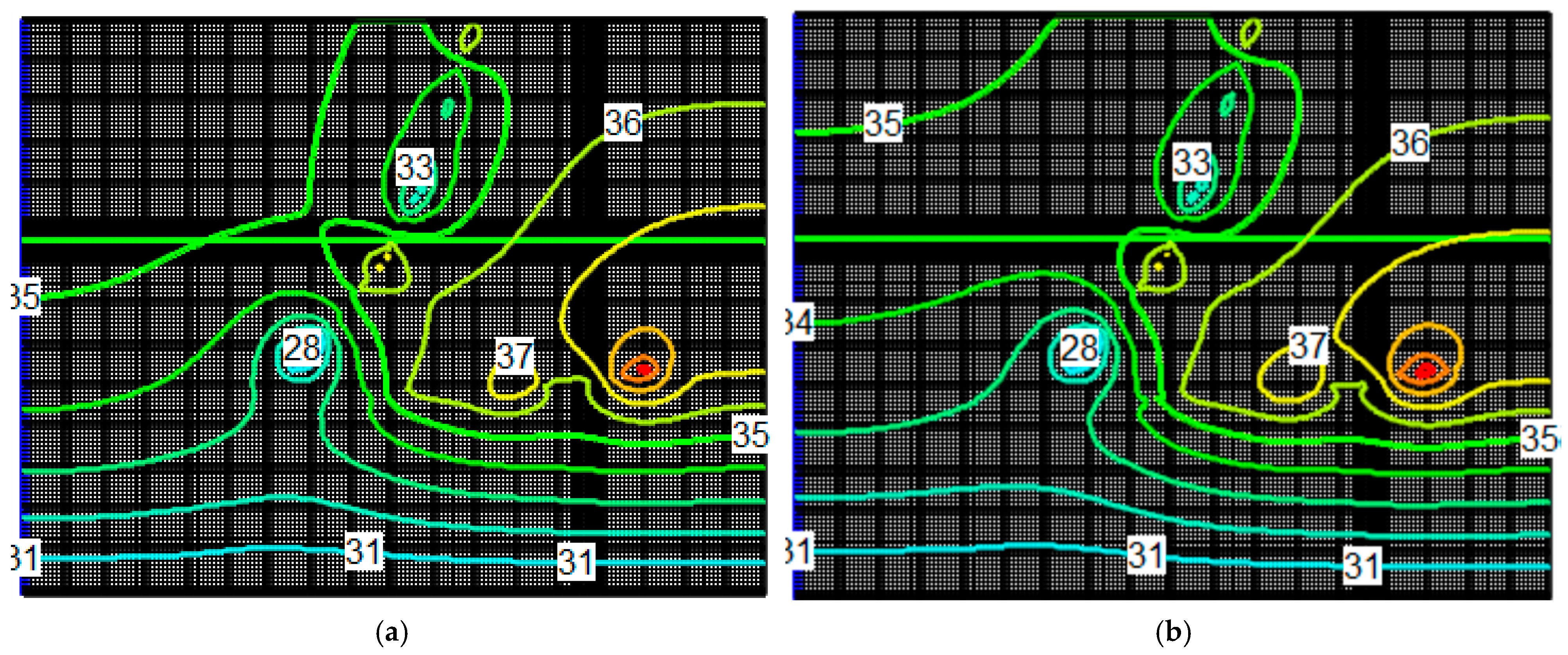
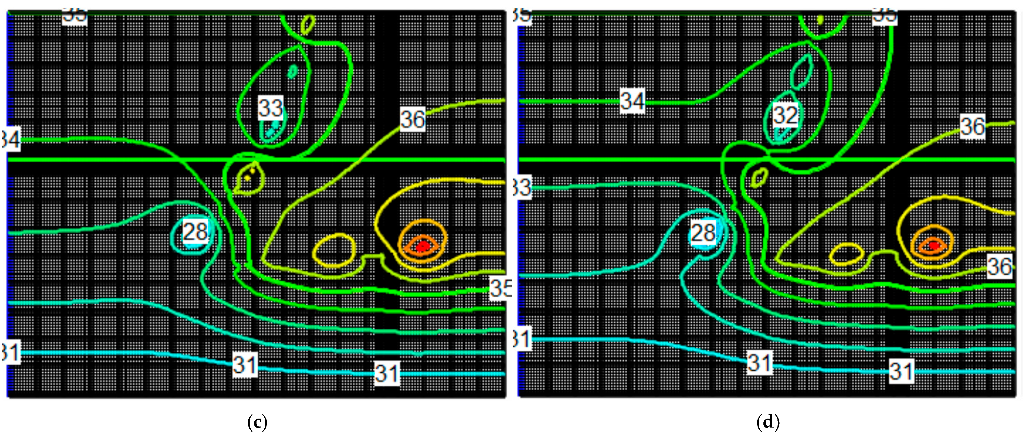
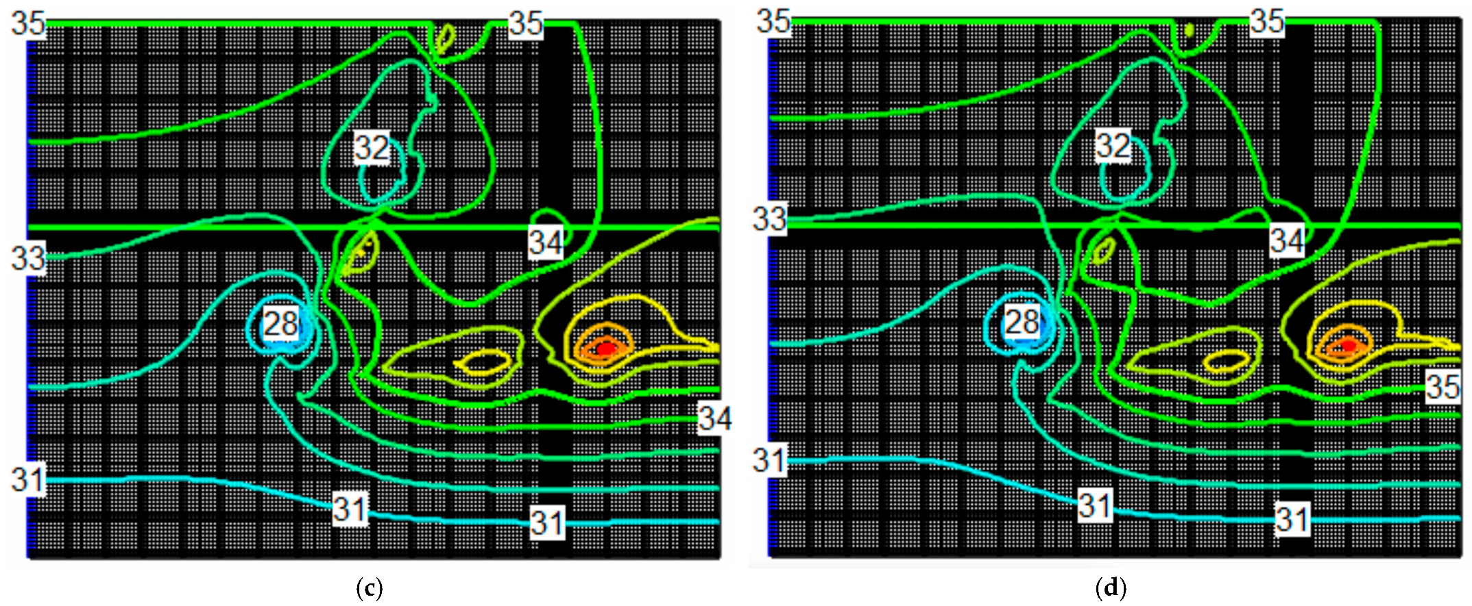
4.3. Steady-State Flow Model
4.4. Transient-State Flow Model
4.5. Dewatering System Performance
4.6. Discussion
5. Conclusions
- The analysis of a numerical model of the “Torre Tres Rios” project in the city of Culiacan, Sinaloa, indicated that the main recharges are induced by the constant load of the water table in the area, as well as the influence of the Tamazula River and precipitation. Additionally, the main discharges include the river and the same constant load of the water table.
- The configuration of the water table suggests that the contribution of the Tamazula River discharges into the Humaya River and is influenced in the area where the project was carried out.
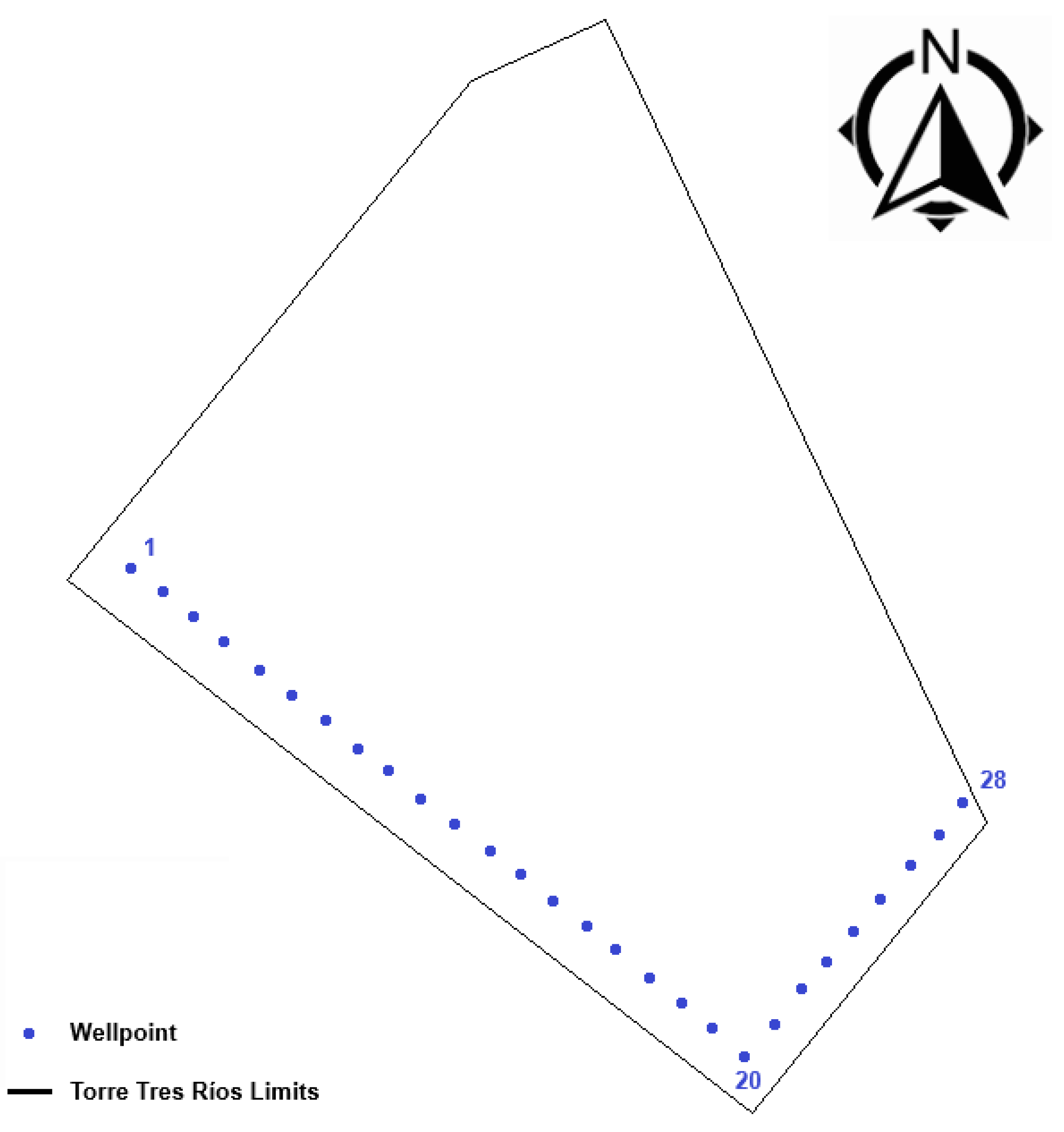
- The wellpoint system model consisted of 28 wells positioned along the flow direction. The wells were spaced 3 m apart with a diameter of 2 inches, as shown in Figure 14. They were connected to a main 6-inch collector and linked to a rotary suction pump with a capacity of 20 HP. In the model, the system reached the excavation level without facing localized overexploitation of the aquifer.
- The observed data from the field, compared with the simulated data, showed that the system controlled the water table at a depth of 6.5m by pumping 28 lps under critical conditions; in contrast, with traditional methods such as deep wells, pumping of 120 lps was needed. In this way, the process was efficient, since the pumping required was considerably reduced (by 75%); also, the pump power was lower, so the hydraulic design had better performance. It also reduced the radius of influence of the drawdown cone and the potential impacts, including overexploitation (excessive pumping rates), which could cause instability in the excavation slopes or settlement of nearby structures.
- The sensitivity and uncertainty analyses confirmed that hydraulic conductivity, transmissivity, and recharge rates were the primary factors influencing groundwater fluctuations in the study area.
- Finally, a model was obtained that achieved the objective of this paper: to evaluate a dewatering system that enabled the construction of the project under optimal conditions and a reduced pumping flow rate. Additionally, the model represents the behavior of the aquifer flow regime, which is altered by the dewatering system. These results provide a reliable basis for informed decision-making in dewatering optimization, allowing for safer and more efficient and sustainable practices in construction.
Author Contributions
Funding
Data Availability Statement
Acknowledgments
Conflicts of Interest
Appendix A
References
- Prontuario Normativo de, la Administración Pública de la Ciudad de México. RCDF: Reglamento de Construcciones del Distrito Federal; Colegio de Ingenieros Municipales: México City, Mexico, 2004. [Google Scholar]
- Gaceta Oficial De La Ciudad De México. Normas Técnicas Complementarias para Diseño y Construcción de Cimentaciones; Gaceta Oficial del Distrito Federal: Mexico City, Mexico, 2004.
- Patrick, J. Powers, Construction Dewatering and Groundwater Control: New Methods and Applications; Wiley: Hoboken, NJ, USA, 2007. [Google Scholar]
- Cashman, P.M.; Preene, M. Groundwater Lowering in Construction: A Practical Guide to Dewatering; CRC Press: Boca Raton, FL, USA; Taylor & Francis Group: Milton Park, UK, 2014. [Google Scholar]
- Somerville, S.H. Control of Groundwater for Temporary Works; Construction Industry Research and Information Association: London, UK, 1986. [Google Scholar]
- Shaqour, F.M.; Hasan, S.E. Groundwater control for construction purposes: A case study from Kuwait. Environ. Geol. 2008, 53, 1603–1612. [Google Scholar] [CrossRef]
- Peck, R.B. Advantages and Limitations of the Observational Method in Applied Soil Mechanics. Géotechnique 1969, 19, 171–187. [Google Scholar] [CrossRef]
- Nicholson, D.; Tse, C.M.; Penny, C.; O Hana, S.; Dimmock, R. The Observational Method in Ground Engineering: Principles and Applications; CIRIA: London, UK, 1999. [Google Scholar]
- Shi, C.; Cao, C.; Lei, M.; Peng, L.; Jiang, J. Optimal design and dynamic control of construction dewatering with the consideration of dewatering process. KSCE J. Civ. Eng. 2017, 21, 1161–1169. [Google Scholar] [CrossRef]
- Pathak, R.; Awasthi, M.K.; Sharma, S.K.; Hardaha, M.K.; Nema, R.K. Ground Water Flow Modelling Using MODFLOW–A Review. Int. J. Curr. Microbiol. Appl. Sci. 2018, 7, 83–88. [Google Scholar] [CrossRef]
- RSun, J.; Johnston, R.H. Regional Aquifer-System Analysis Program of the US Geological Survey; US Government Printing Office: Washington, DC, USA, 1994; Volume 1099.
- Harbaugh, A.W.; Banta, E.R.; Hill, M.C.; Mcdonald, M.G. MODFLOW-2000, the US Geological Survey Modular Ground-Water Model: User Guide to Modularization Concepts and the Ground-Water Flow Process; McDonald Morrissey Associates: Concord, NH, USA, 2000. [Google Scholar]
- Harbaugh, A.W. MODFLOW-2005: The U.S. Geological Survey Modular Ground-Water Model-the Ground-Water Flow Process. Available online: https://www.semanticscholar.org/paper/MODFLOW-2005-%3A-the-U.S.-Geological-Survey-modular-Harbaugh/8f66c41c163e48f97c00319045275210c8556ae1 (accessed on 31 December 2024).
- Carrera, J.; Neuman, S.P. Estimation of Aquifer Parameters Under Transient and Steady State Conditions: 1. Maximum Likelihood Method Incorporating Prior Information. Water Resour. Res. 1986, 22, 199–210. [Google Scholar] [CrossRef]
- Dai, Z.; Samper, J. Inverse problem of multicomponent reactive chemical transport in porous media: Formulation and applications. Water Resour. Res. 2004, 40. [Google Scholar] [CrossRef]
- Dai, Z.; Samper, J. Inverse modeling of water flow and multicomponent reactive transport in coastal aquifer systems. J. Hydrol. 2006, 327, 447–461. [Google Scholar] [CrossRef]
- Shang, H.; Wang, W.; Dai, Z.; Duan, L.; Zhao, Y.; Zhang, J. An ecology-oriented exploitation mode of groundwater resources in the northern Tianshan Mountains, China. J. Hydrol. 2016, 543, 386–394. [Google Scholar] [CrossRef]
- Carrillo, N. Influence of Artesian Wells in the Sinking of Mexico City. In Proceedings of the 2nd International Conference on Soils Mechanics, Rotterdam, The Netherlands, 21–30 June 1948. [Google Scholar]
- Ortega-Guerrero, A.; Cherry, J.A.; Rudolph, D.L. Large-Scale Aquitard Consolidation Near Mexico City. Groundwater 1993, 31, 708–718. [Google Scholar] [CrossRef]
- Avilés, J.; Pérez-Rocha, L.E. Regional subsidence of Mexico City and its effects on seismic response. Soil Dyn. Earthq. Eng. 2010, 30, 981–989. [Google Scholar] [CrossRef]
- Powrie, W.; Roberts, T.O.L.; Moghazy, H.E.D. Effects of high permeability lenses on efficiency of wellpoint dewatering. Géotechnique 1989, 39, 543–547. [Google Scholar] [CrossRef]
- Huang, C.; Mayer, A.S. Pump-and-treat optimization using well locations and pumping rates as decision variables. Water Resour. Res. 1997, 33, 1001–1012. [Google Scholar] [CrossRef]
- Larson, K.J.; Başaǧaoǧlu, H.; Mariño, M.A. Prediction of optimal safe ground water yield and land subsidence in the Los Banos-Kettleman City area, California, using a calibrated numerical simulation model. J. Hydrol. 2001, 242, 79–102. [Google Scholar] [CrossRef]
- Leighton, D.A.; Phillips, S.P. Simulation of Ground-Water Flow and Land Subsidence in the Antelope Valley Ground-Water Basin, California; Water-Resources Investigations Report 03-4016; U.S. Geological Survey: Reston, VA, USA, 2003.
- Xu, Y.-S.; Ma, L.; Shen, S.-L.; Sun, W.-J. Evaluation of land subsidence by considering underground structures that penetrate the aquifers of Shanghai, China. Hydrogeol. J. 2012, 20, 1623–1634. [Google Scholar] [CrossRef]
- Pujades, E.; López, A.; Carrera, J.; Vázquez-Suñé, E.; Jurado, A. Barrier effect of underground structures on aquifers. Eng. Geol. 2012, 145, 41–49. [Google Scholar] [CrossRef]
- Surinaidu, L.; Rao, V.V.S.G.; Rao, N.S.; Srinu, S. Hydrogeological and groundwater modeling studies to estimate the groundwater inflows into the coal Mines at different mine development stages using MODFLOW, Andhra Pradesh, India. Water Resour. Ind. 2014, 7–8, 49–65. [Google Scholar] [CrossRef]
- Pujades, E.; De Simone, S.; Carrera, J.; Vázquez-Suñé, E.; Jurado, A. Settlements around pumping wells: Analysis of influential factors and a simple calculation procedure. J. Hydrol. 2017, 548, 225–236. [Google Scholar] [CrossRef]
- Zeng, C.-F.; Wang, S.; Xue, X.-L.; Zheng, G.; Mei, G.-X. Evolution of deep ground settlement subject to groundwater drawdown during dewatering in a multi-layered aquifer-aquitard system: Insights from numerical modelling. J. Hydrol. 2021, 603, 127078. [Google Scholar] [CrossRef]
- Pujades, E.; Jurado, A.; Carrera, J.; Vázquez-Suñé, E.; Dassargues, A. Hydrogeological assessment of non-linear underground enclosures. Eng. Geol. 2016, 207, 91–102. [Google Scholar] [CrossRef]
- Feng, Q.; Zhan, H. Constant-head test at a partially penetrating well in an aquifer-aquitard system. J. Hydrol. 2019, 569, 495–505. [Google Scholar] [CrossRef]
- Wang, J.; Liu, X.; Wu, Y.; Liu, S.; Wu, L.; Lou, R.; Lu, J.; Yin, Y. Field experiment and numerical simulation of coupling non-Darcy flow caused by curtain and pumping well in foundation pit dewatering. J. Hydrol. 2017, 549, 277–293. [Google Scholar] [CrossRef]
- Subdirección General Técnica Gerencia de Aguas Subterráneas. Available online: https://www.gob.mx/cms/uploads/attachment/file/100875/GAS_Acuerdo_6._Comisi_n_intersecretarial.pdf (accessed on 23 February 2025).
- CONAGUA. Determinación de la Disponibilidad de Agua en el Acuífero Río Culiacán, Estado de Sinaloa; Diario Oficial de la Federación: Mexico City, Mexico, 2013. Available online: https://www.gob.mx/cms/uploads/attachment/file/103342/DR_2504.pdf (accessed on 31 December 2024).
- De Cueto-Díaz, D.J. Estudio de Mecánica de Suelos para la Torre de Dieciséis Niveles; Geotechnical Study Report; Centro Experimental y Servicios en Ingeniería Civil: Culiacán, Mexico, 2009. [Google Scholar]
- Hidalgo-Pérez, J. Optimización de un abatimiento del nivel freático para una excavación mediante el programa Modflow; Escuela Técnica Superior de Ingeniería: Cartagena, Colombia, 2015. [Google Scholar]
- Preene, M.; Roberts, T.; Powrie, W. Groundwater Control: Design and Practice, 2nd ed.; CIRIA: London, UK, 2016; Available online: www.ciria.org (accessed on 31 December 2024).
- Darcy, H. Les Fontaines Publiques de la Ville de Dijon; Gallica: Paris, France, 1856. [Google Scholar]
- Bear, J. Dynamics of Fluids in Porous Media; Dover Publications: Garden City, NY, USA, 2013. [Google Scholar]
- Anderson, M.P.; Woessner, W.W.; Hunt, R.J. Applied Groundwater Modeling: Simulation of Flow and Advective Transport; Academic Press: Cambridge, MA, USA, 2015. [Google Scholar]
- Khosravi, M.; Khosravi, M.H.; Najafabadi, S.H.G. Determining the portion of dewatering-induced settlement in excavation pit projects. Int. J. Geotech. Eng. 2021, 15, 563–573. [Google Scholar] [CrossRef]
- Wu, Y.-X.; Lyu, H.-M.; Han, J.; Shen, S.-L. Dewatering–Induced Building Settlement around a Deep Excavation in Soft Deposit in Tianjin, China. J. Geotech. Geoenvironmental Eng. 2019, 145, 05019003. [Google Scholar] [CrossRef]
- Chen, Z.; Huang, J.; Zhan, H.; Wang, J.; Dou, Z.; Zhang, C.; Chen, C.; Fu, Y. Optimization schemes for deep foundation pit dewatering under complicated hydrogeological conditions using MODFLOW-USG. Eng. Geol. 2022, 303, 06653. [Google Scholar] [CrossRef]


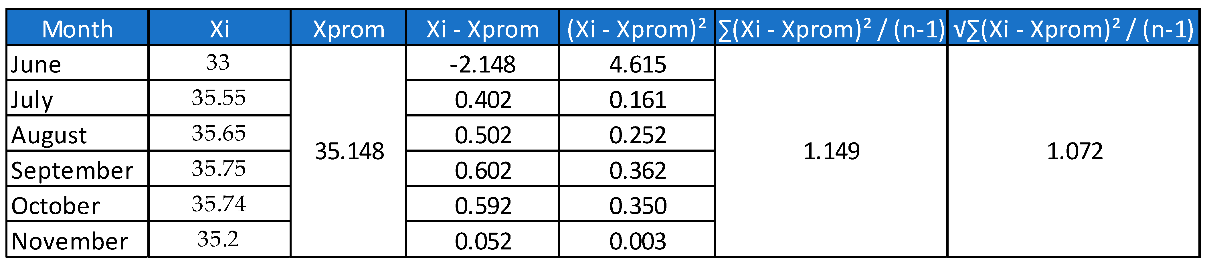
| Month | Observed Water Table (masl) | Depth (m) |
|---|---|---|
| June | 33.00 | 7.00 |
| July | 35.55 | 4.45 |
| August | 35.65 | 4.35 |
| September | 35.75 | 4.25 |
| October | 35.74 | 4.26 |
| November | 35.20 | 4.80 |
| Month | Tamazula River Discharge Rate (m3/s) | Month | Humaya River Discharge Rate (m3/s) |
|---|---|---|---|
| June | 20.00 | June | 89.56 |
| July | 19.83 | July | 100.27 |
| August | 25.56 | August | 99.34 |
| September | 31.52 | September | 97.50 |
| October | 26.31 | October | 98.94 |
| November | 19.85 | November | 72.39 |
| Torre Tres Ríos | |
|---|---|
| Aquifer | Unconfined, heterogeneous, anisotropic |
| Aquifer depth | 40 m |
| System outflows | Rivers and pumping |
| System inflows | Rivers and precipitation |
| Water table level | Variable (33–35.74 masl) |
| Excavation level | 33.5 masl |
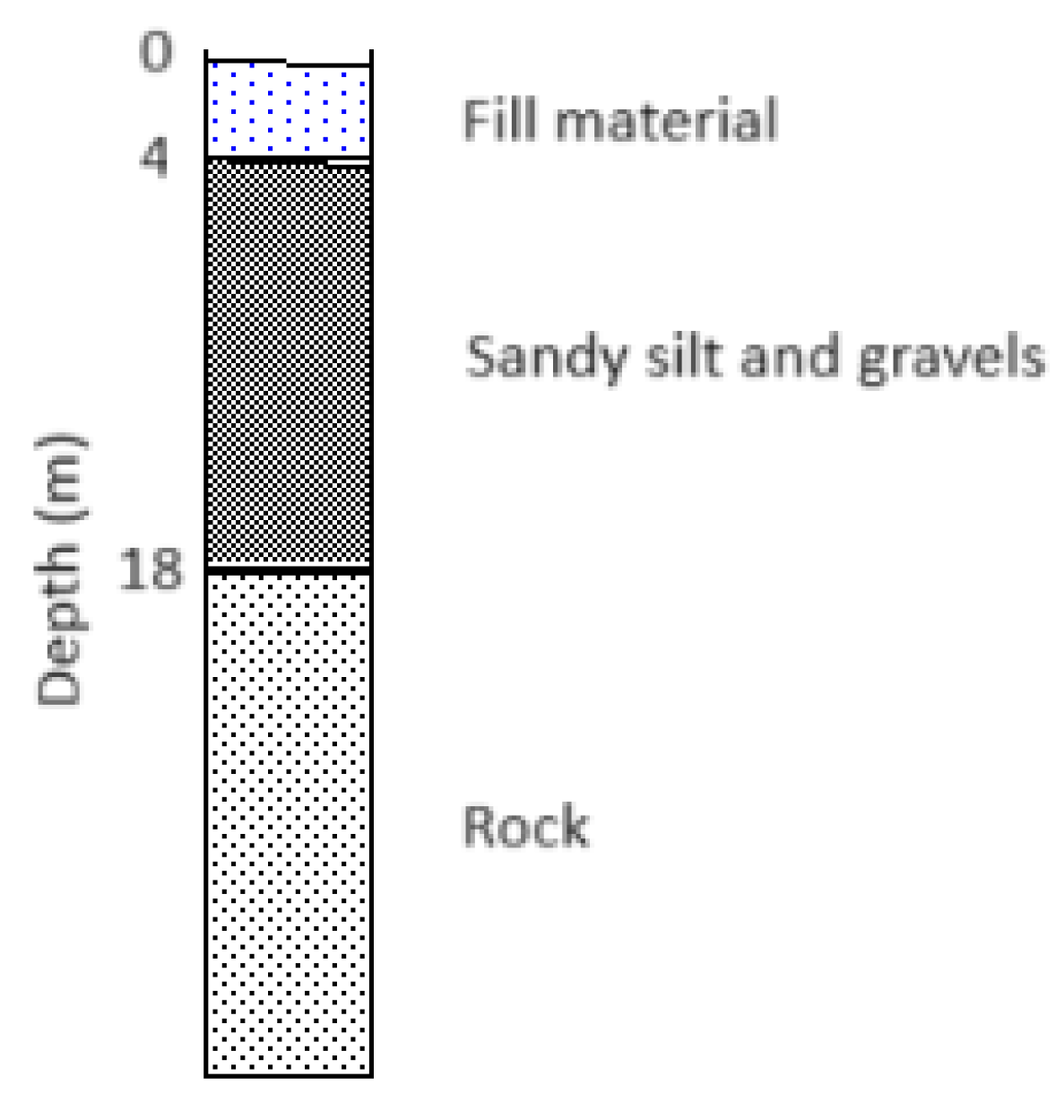
| Stratigraphy | Fill material, alluviofluvial, rock |
| Parameter | Baseline Value | Variation Range | Sensitivity (∆h) | Influence |
|---|---|---|---|---|
| Hydraulic conductivity (Kx, Ky) | 3.24 × 10⁻⁴ m/s | 1 × 10⁻⁵ to 5 × 10⁻⁴ m/s | ±1.5 m | High |
| Transmissivity | 470 m2/day | 280.1 to 843.3 m2/day | ±1.2 m | Moderate–High |
| Recharge from precipitation | 10% of rainfall (Figure 7) | 5 to 15% | ±1.8 m | High |
| River flow influence | BANDAS database (Table 2) | ±15% variation in average flow | ±0.7 m | Moderate |
| Month | Mean Water Table (masl) | Standard Deviation (m) | 95% Confidence Interval (masl) |
|---|---|---|---|
| June | 33.00 | 0.72 | 32.3–33.7 |
| July | 35.55 | 0.80 | 34.8–36.3 |
| August | 35.65 | 0.84 | 34.9–36.5 |
| September | 35.75 | 0.88 | 34.9–36.6 |
| October | 35.74 | 0.85 | 34.9–36.6 |
| November | 35.20 | 0.92 | 34.3–36.1 |
| Month | Observed Water Table | Modeled Water Table | Residual |
|---|---|---|---|
| June | 33.00 | 32.725 | −0.275 |
| July | 35.55 | 35.675 | 0.125 |
| August | 35.65 | 35.850 | 0.200 |
| September | 35.75 | 36.025 | 0.275 |
| October | 35.74 | 35.676 | −0.064 |
| November | 35.2 | 35.438 | 0.238 |
| Month | Wellpoint Flow Rate (lps) | Deep Well Flow Rate (lps) |
|---|---|---|
| July | 22.4 | 89.3 |
| August * | 28 | 120 |
| September * | 25.76 | 99.52 |
| October | 22.4 | 89.3 |
| November | 19.6 | 85 |
| December | 19.6 | 85 |
| Month | Wellpoint Flow Rate (lps) | Radius of Influence (m) | Deep Well Flow Rate (lps) | Radius of Influence (m) |
|---|---|---|---|---|
| August | 28 | 14 | 120 | 60 |
| September | 25.76 | 12.26 | 99.52 | 47.43 |
Disclaimer/Publisher’s Note: The statements, opinions and data contained in all publications are solely those of the individual author(s) and contributor(s) and not of MDPI and/or the editor(s). MDPI and/or the editor(s) disclaim responsibility for any injury to people or property resulting from any ideas, methods, instructions or products referred to in the content. |
© 2025 by the authors. Licensee MDPI, Basel, Switzerland. This article is an open access article distributed under the terms and conditions of the Creative Commons Attribution (CC BY) license (https://creativecommons.org/licenses/by/4.0/).
Share and Cite
Beltrán-Vargas, D.; García-Páez, F.; Martínez-Morales, M.; Rentería-Guevara, S.A. Novel Numerical Modeling of a Groundwater Level-Lowering Approach Implemented in the Construction of High-Rise/Complex Buildings. Water 2025, 17, 732. https://doi.org/10.3390/w17050732
Beltrán-Vargas D, García-Páez F, Martínez-Morales M, Rentería-Guevara SA. Novel Numerical Modeling of a Groundwater Level-Lowering Approach Implemented in the Construction of High-Rise/Complex Buildings. Water. 2025; 17(5):732. https://doi.org/10.3390/w17050732
Chicago/Turabian StyleBeltrán-Vargas, David, Fernando García-Páez, Manuel Martínez-Morales, and Sergio A. Rentería-Guevara. 2025. "Novel Numerical Modeling of a Groundwater Level-Lowering Approach Implemented in the Construction of High-Rise/Complex Buildings" Water 17, no. 5: 732. https://doi.org/10.3390/w17050732
APA StyleBeltrán-Vargas, D., García-Páez, F., Martínez-Morales, M., & Rentería-Guevara, S. A. (2025). Novel Numerical Modeling of a Groundwater Level-Lowering Approach Implemented in the Construction of High-Rise/Complex Buildings. Water, 17(5), 732. https://doi.org/10.3390/w17050732