
Prewhitening-Aided Innovative Trend Analysis Method for Trend Detection in Hydrometeorological Time Series


Abstract

1. Introduction
2. Brief Description of ITA Method
2.1. Innovation Trend Analysis (ITA)
2.2. Improved ITA Method Based on Covariance (COV_ITA)
2.3. Improved ITA Method Based on Bootstrap Method (Bootstrap_ITA)
- (1)
- Divide the time series data into two sub-series with equal size, and arrange them in an ascending order to calculate P in Equation (8);
- (2)
- Randomly select n sample data (some of which may be sampled multiple times) from to form a new sample time series. After resampling M times, arrange the obtained new indicators in ascending order as: ;
- (3)
- Given significance level α, calculate ,, and then the confidence interval is . If the indicator P falls in the confidence interval, the trend is not significant at the significance level α; otherwise, it is considered significant; besides, p > 0 represents an upward trend, while p < 0 represents a downward trend.
2.4. ITA Method Based on Variance Correction Analysis (VCA_ITA)
3. Prewhitening-Aided ITA Method
3.1. Correction of Formula in ITA
3.2. Combination of Corrected ITA Method and Prewhitening Methods
- (1)
- Use the Theil Sen Median method (TSA) [13] to calculate the linear trend slope of the original time series Xt = (X1, X2, … Xn):where b is the calculated linear trend slope, “Median” is the median function, and Xi is the i-th observation value.
- (2)
- Choose an appropriate prewhitening method to handle the original time series Xt.
- (3)
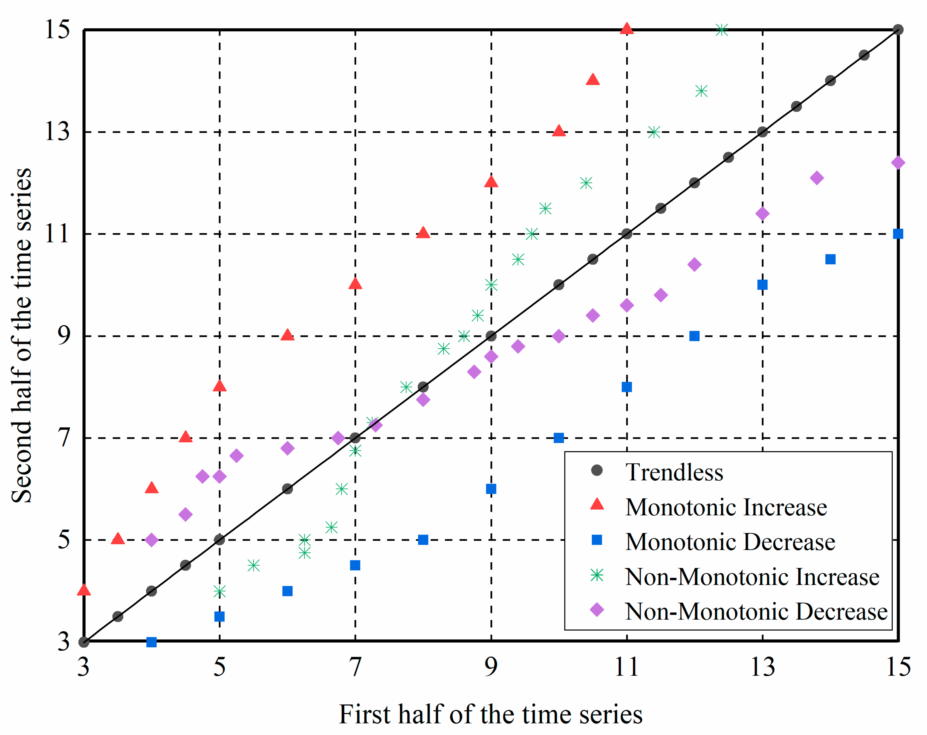
- Follow the steps of the ITA method to first divide the prewhitened time series into equal parts and arrange them in ascending order. Then, take the first and second halves as the abscissa and ordinate, respectively, to draw a scatter plot in the Cartesian coordinate system (Figure 1). If the scattered points are distributed above (below) the 45° line, it indicates a monotonic upward (downward) trend. If the scattered points are distributed near the 45° line, it indicates an insignificant trend.
- (4)
- Use Equation (16) to calculate the corrected standard deviation of the trend slope in the prewhitened time series.
- (5)
- Conduct trend significance assessment. Combine Equations (16) and (1) to obtain the value of ZITA. If , it is considered that the trend is significant at the significance level α, and represents a positive (upward) trend, and represents a negative (downward) trend. In this study, the significance level of α = 0.05 was used.
4. Monte–Carlo Experiments
4.1. Design of Monte–Carlo Experiments
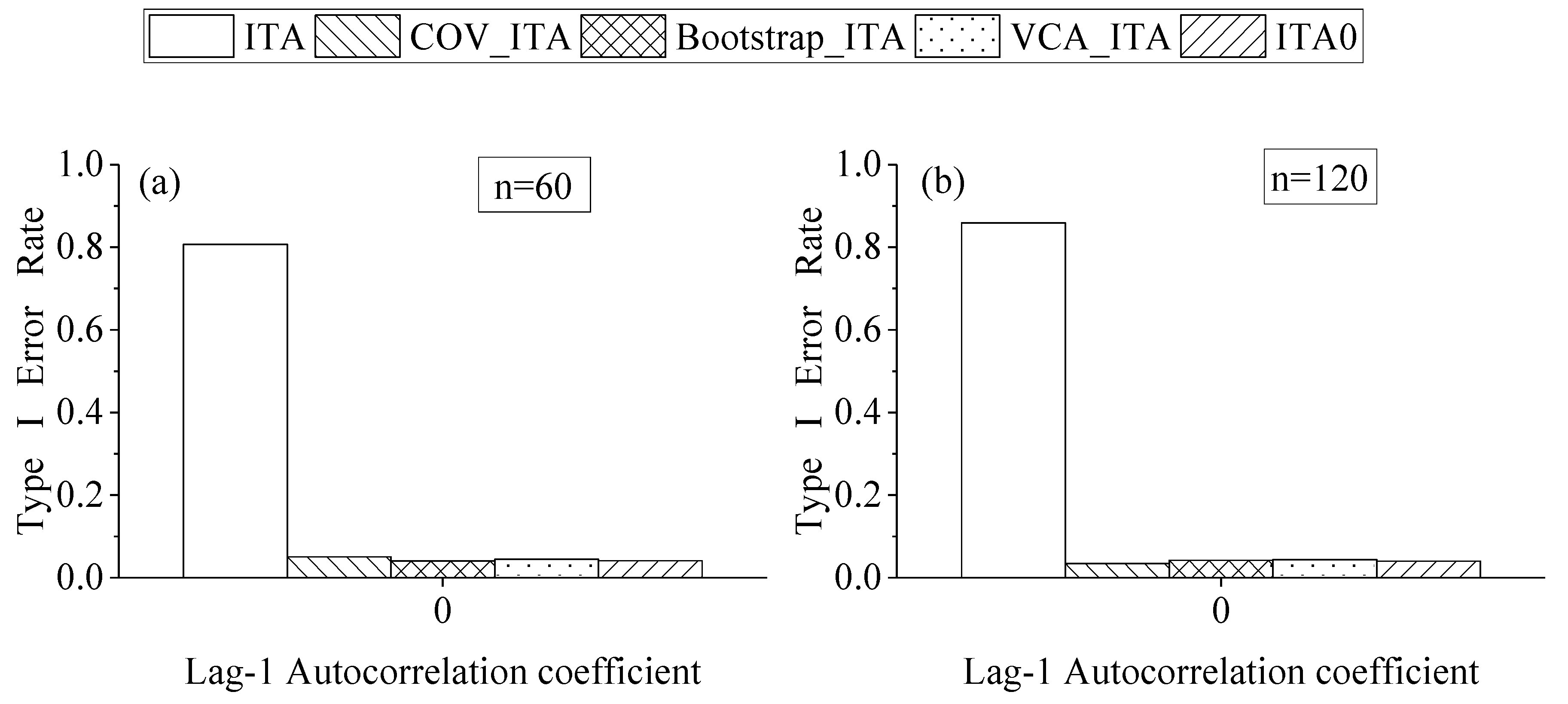
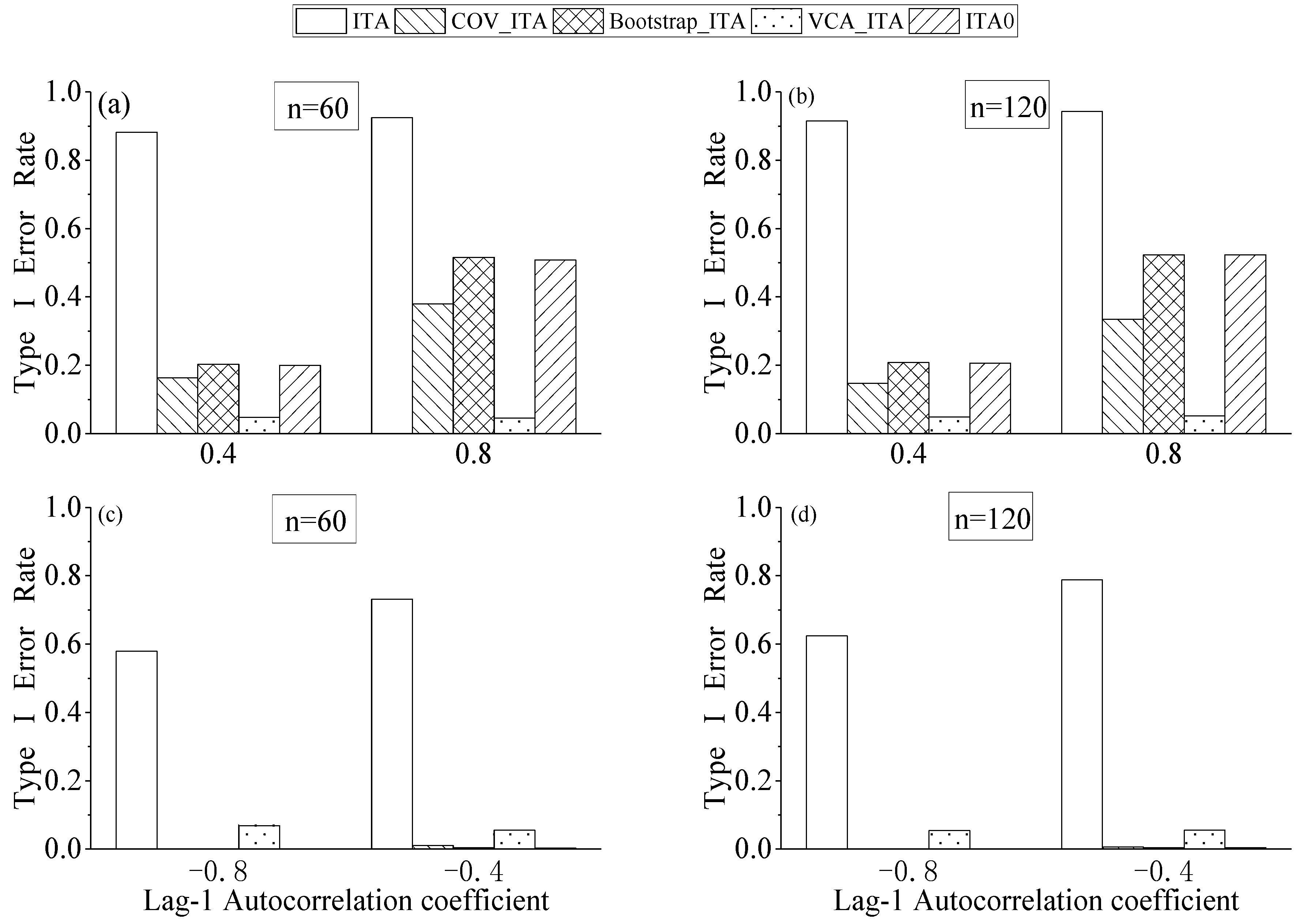
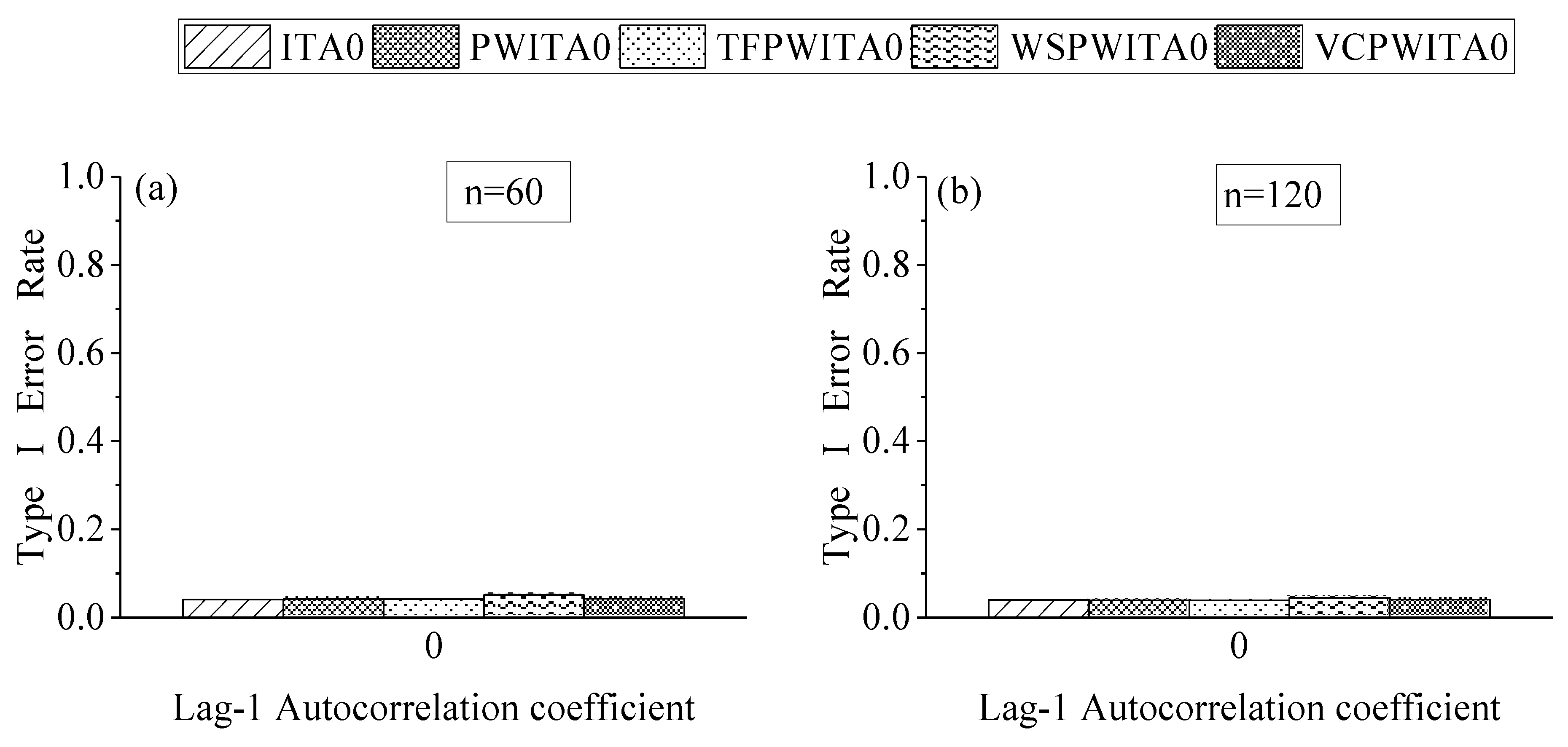
4.2. Effect of Formula Correction in ITA
5. Case Study
6. Conclusions
Author Contributions
Funding
Data Availability Statement
Conflicts of Interest
Abbreviations
| ITA | Innovation trend analysis method |
| COV_ITA | Improved ITA method based on covariance |
| Bootstrap_ITA | Improved ITA method based on bootstrap method |
| VCA_ITA | ITA method based on variance correction analysis |
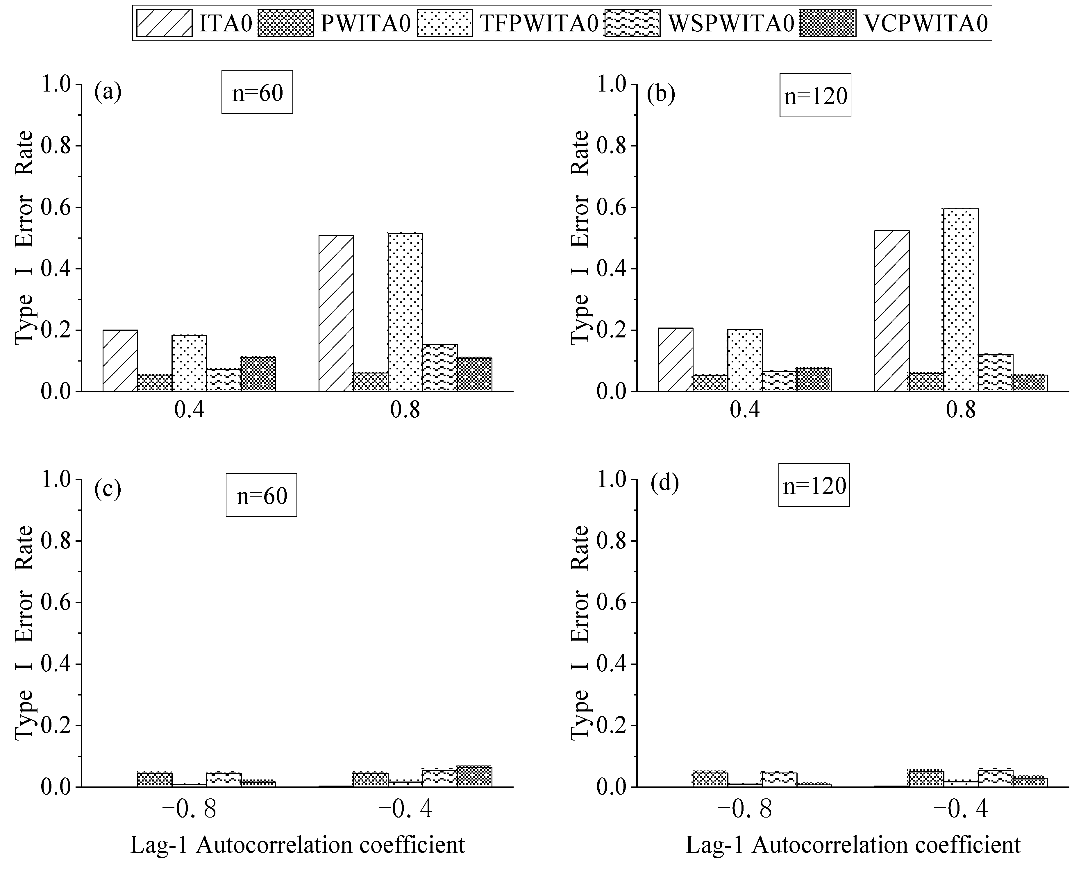
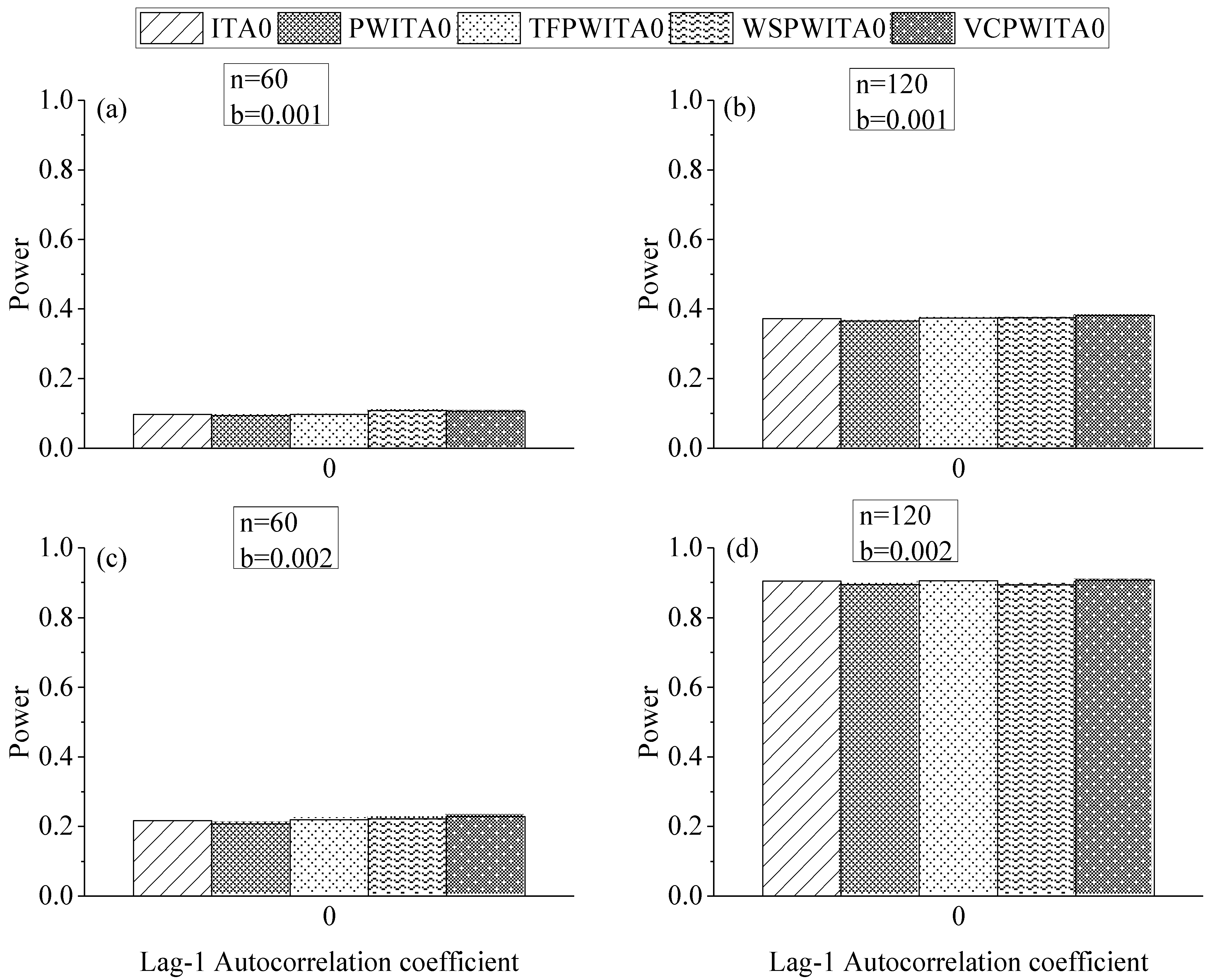
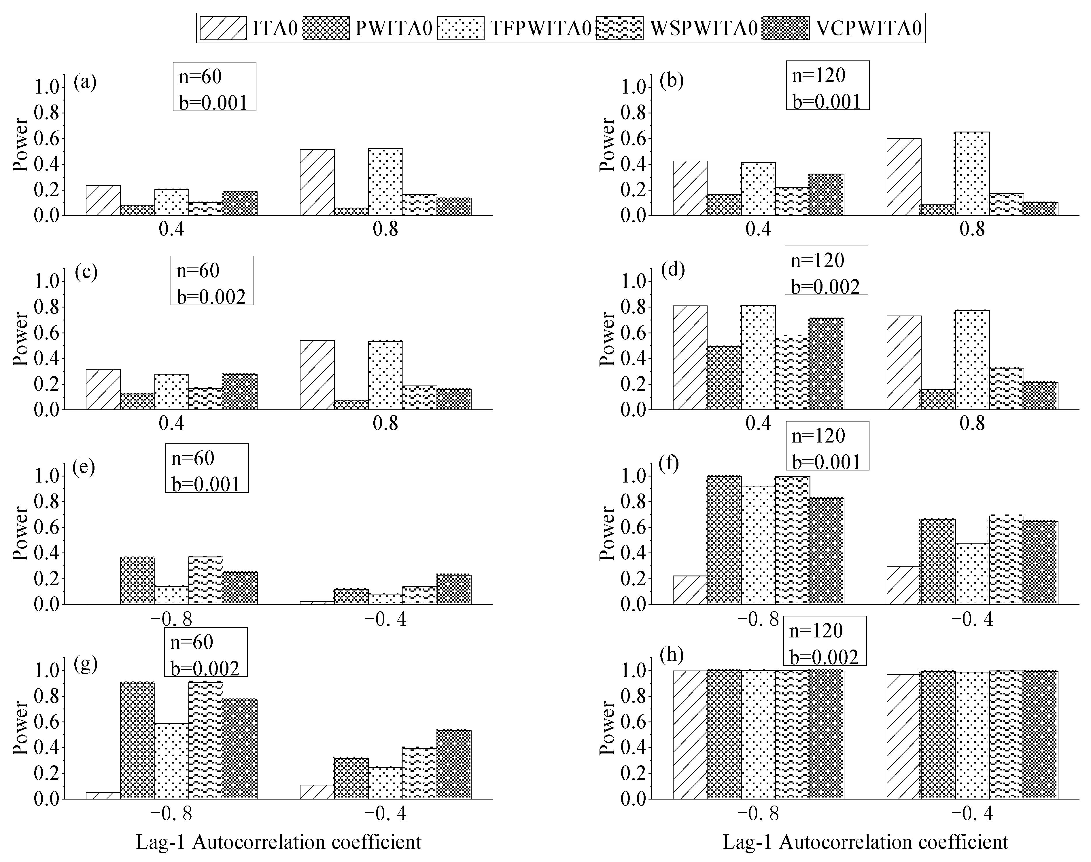
| ITA0 | Only correct the mathematical formula of the original ITA method |
| PWITA0 | Ordinary prewhitening-aided ITA method |
| TFPWITA0 | Trend-free prewhitening-aided ITA method |
| WSPWITA0 | Iterative prewhitening-aided ITA method |
| VCPWITA0 | Variance-corrected prewhitening-aided ITA method |
Appendix A. Four Prewhitening Methods
Appendix A.1. Ordinary Prewhitening (PW) Method
Appendix A.2. Trend-Free Prewhitening (TFPW) Method
- (1)
- Estimate Sen’s slope in the original time series;
- (2)
- According to Equation (A2), remove the trend components from the original time series to obtain the detrended time series ;
- (3)
- According to Equation (A3), remove the autocorrelation from the detrended time series to obtain ;
- (4)
- Add the trend components to to generate the time series for evaluating the statistical significance of its trend.The TFPW method tends to generate Type I errors.
Appendix A.3. Wang and Swail Prewhitening (WSPW) Method
- (1)
- Remove from the original time series and correct the prewhitened data according to Equation (A5);
- (2)
- Estimate Sen’s slope of prewhitened time series ;
- (3)
- Remove the estimated trend () from the original time series to obtain the prewhitened and detrend time series (Equation (A6));
- (4)
- Repeat steps (1)–(3) until the r1 value and the trend slope differences become less than a specified small threshold such as 0.0001, i.e., and (Equations (A7) and (A8)).
Appendix A.4. Variance Correction Prewhitening (VCPW) Method
References
- Imbers, J.; Lopez, A.; Huntingford, C.; Allen, M. Sensitivity of Climate Change Detection and Attribution to the Characterization of Internal Climate Variability. J. Clim. 2014, 27, 3477–3491. [Google Scholar] [CrossRef]
- Liebmann, B.; Dole, R.M.; Jones, C.; Bladé, I.; Allured, D. Influence of Choice of Time Period on Global Surface Temperature Trend Estimates. Bull. Am. Meteorol. Soc. 2010, 91, 1485–1492. [Google Scholar] [CrossRef]
- Khaliq, M.N.; Ouarda, T.B.; Gachon, P.; Sushama, L.; St-Hilaire, A. Identification of Hydrological Trends in the Presence of Serial and Cross Correlations: A Review of Selected Methods and Their Application to Annual Flow Regimes of Canadian Rivers. J. Hydrol. 2009, 368, 117–130. [Google Scholar] [CrossRef]
- Sonali, P.; Kumar, D.N. Review of Trend Detection Methods and Their Application to Detect Temperature Changes in India. J. Hydrol. 2013, 476, 212–227. [Google Scholar] [CrossRef]
- Pandey, B.K.; Khare, D.; Tiwari, H.; Mishra, P.K. Analysis and Visualization of Meteorological Extremes in Humid Subtropical Regions. Nat. Hazards 2021, 108, 661–687. [Google Scholar] [CrossRef]
- Ma, D.; Wang, T.; Gao, C.; Pan, S.; Sun, Z.; Xu, Y.-P. Potential Evapotranspiration Changes in Lancang River Basin and Yarlung Zangbo River Basin, Southwest China. Hydrol. Sci. J. 2018, 63, 1653–1668. [Google Scholar] [CrossRef]
- Şan, M.; Akçay, F.; Linh, N.T.T.; Kankal, M.; Pham, Q.B. Innovative and Polygonal Trend Analyses Applications for Rainfall Data in Vietnam. Theor. Appl. Climatol. 2021, 144, 809–822. [Google Scholar] [CrossRef]
- Madsen, H.; Lawrence, D.; Lang, M.; Martinkova, M.; Kjeldsen, T.R. Review of Trend Analysis and Climate Change Projections of Extreme Precipitation and Floods in Europe. J. Hydrol. 2014, 519, 3634–3650. [Google Scholar] [CrossRef]
- Li, X.; Sang, Y.-F.; Sivakumar, B.; Gil-Alana, L.A. Detection of Type of Trends in Surface Air Temperature in China. J. Hydrol. 2021, 596, 126061. [Google Scholar] [CrossRef]
- Kendall, M.G. A New Measure of Rank Correlation. Biometrika 1938, 30, 81–93. [Google Scholar] [CrossRef]
- Mann, H.B. Nonparametric Tests against Trend. Econom. J. Econom. Soc. 1945, 13, 245–259. [Google Scholar] [CrossRef]
- Lehmann, E.L.; D’Abrera, H.J. Nonparametrics: Statistical Methods Based on Ranks; Springer: New York, NY, USA, 2006; Volume 464. [Google Scholar]
- Sen, P.K. Estimates of the Regression Coefficient Based on Kendall’s Tau. J. Am. Stat. Assoc. 1968, 63, 1379–1389. [Google Scholar] [CrossRef]
- Güçlü, Y.S. Improved Visualization for Trend Analysis by Comparing with Classical Mann-Kendall Test and ITA. J. Hydrol. 2020, 584, 124674. [Google Scholar] [CrossRef]
- Sang, Y.-F.; Sun, F.; Singh, V.P.; Xie, P.; Sun, J. A Discrete Wavelet Spectrum Approach for Identifying Non-Monotonic Trends in Hydroclimate Data. Hydrol. Earth Syst. Sci. 2018, 22, 757–766. [Google Scholar] [CrossRef]
- Sang, Y.-F.; Sivakumar, B.; Zhang, Y. Is There an Underestimation of Long-Term Variability of Streamflow across the Continental United States? J. Hydrol. 2020, 581, 124365. [Google Scholar] [CrossRef]
- Sang, Y.; Singh, V.P.; Wen, J.; Liu, C. Gradation of Complexity and Predictability of Hydrological Processes. J. Geophys. Res. Atmos. 2015, 120, 5334–5343. [Google Scholar] [CrossRef]
- Yue, S.; Pilon, P.; Phinney, B.; Cavadias, G. The Influence of Autocorrelation on the Ability to Detect Trend in Hydrological Series. Hydrol. Process. 2002, 16, 1807–1829. [Google Scholar] [CrossRef]
- Yue, S.; Pilon, P.; Phinney, B. Canadian Streamflow Trend Detection: Impacts of Serial and Cross-Correlation. Hydrol. Sci. J. 2003, 48, 51–63. [Google Scholar] [CrossRef]
- Kisi, O.; Ay, M. Comparison of Mann–Kendall and Innovative Trend Method for Water Quality Parameters of the Kizilirmak River, Turkey. J. Hydrol. 2014, 513, 362–375. [Google Scholar] [CrossRef]
- Wang, Y.; Xu, Y.; Tabari, H.; Wang, J.; Wang, Q.; Song, S.; Hu, Z. Innovative Trend Analysis of Annual and Seasonal Rainfall in the Yangtze River Delta, Eastern China. Atmos. Res. 2020, 231, 104673. [Google Scholar] [CrossRef]
- Wang, W.; Chen, Y.; Becker, S.; Liu, B. Variance Correction Prewhitening Method for Trend Detection in Autocorrelated Data. J. Hydrol. Eng. 2015, 20, 04015033. [Google Scholar] [CrossRef]
- Şen, Z. Innovative Trend Analysis Methodology. J. Hydrol. Eng. 2012, 17, 1042–1046. [Google Scholar] [CrossRef]
- Şen, Z. Innovative Trend Significance Test and Applications. Theor. Appl. Climatol. 2017, 127, 939–947. [Google Scholar] [CrossRef]
- Kisi, O. An Innovative Method for Trend Analysis of Monthly Pan Evaporations. J. Hydrol. 2015, 527, 1123–1129. [Google Scholar] [CrossRef]
- Tabari, H.; Taye, M.T.; Onyutha, C.; Willems, P. Decadal Analysis of River Flow Extremes Using Quantile-Based Approaches. Water Resour. Manag. 2017, 31, 3371–3387. [Google Scholar] [CrossRef]
- Wang, W.; Zhu, Y.; Liu, B.; Chen, Y.; Zhao, X. Innovative Variance Corrected Sen’s Trend Test on Persistent Hydrometeorological Data. Water 2019, 11, 2119. [Google Scholar] [CrossRef]
- Serinaldi, F.; Chebana, F.; Kilsby, C.G. Dissecting Innovative Trend Analysis. Stoch. Environ. Res. Risk Assess. 2020, 34, 733–754. [Google Scholar] [CrossRef]
- Zhou, Z.; Wang, L.; Lin, A.; Zhang, M.; Niu, Z. Innovative Trend Analysis of Solar Radiation in China during 1962–2015. Renew. Energy 2018, 119, 675–689. [Google Scholar] [CrossRef]
- Li, J.; Wu, W.; Ye, X.; Jiang, H.; Gan, R.; Wu, H.; He, J.; Jiang, Y. Innovative Trend Analysis of Main Agriculture Natural Hazards in China during 1989–2014. Nat. Hazards 2019, 95, 677–720. [Google Scholar] [CrossRef]
- Alifujiang, Y.; Abuduwaili, J.; Maihemuti, B.; Emin, B.; Groll, M. Innovative Trend Analysis of Precipitation in the Lake Issyk-Kul Basin, Kyrgyzstan. Atmosphere 2020, 11, 332. [Google Scholar] [CrossRef]
- Zerouali, B.; Elbeltagi, A.; Al-Ansari, N.; Abda, Z.; Chettih, M.; Santos, C.A.G.; Boukhari, S.; Araibia, A.S. Improving the Visualization of Rainfall Trends Using Various Innovative Trend Methodologies with Time–Frequency-Based Methods. Appl. Water Sci. 2022, 12, 207. [Google Scholar] [CrossRef]
- Wu, H.; Li, X.; Qian, H.; Chen, J. Improved Partial Trend Method to Detect Rainfall Trends in Hainan Island. Theor. Appl. Climatol. 2019, 137, 2539–2547. [Google Scholar] [CrossRef]
- Alashan, S. Testing and Improving Type 1 Error Performance of Şen’s Innovative Trend Analysis Method. Theor. Appl. Climatol. 2020, 142, 1015–1025. [Google Scholar] [CrossRef]
- Von Storch, H. Misuses of Statistical Analysis in Climate Research. In Analysis of Climate Variability; Von Storch, H., Navarra, A., Eds.; Springer: Berlin/Heidelberg, Germany, 1999; pp. 11–26. ISBN 978-3-642-08560-4. [Google Scholar]
- Wang, X.L.; Swail, V.R. Changes of Extreme Wave Heights in Northern Hemisphere Oceans and Related Atmospheric Circulation Regimes. J. Clim. 2001, 14, 2204–2221. [Google Scholar] [CrossRef]
- Zhang, X.; Zwiers, F.W. Comment on “Applicability of Prewhitening to Eliminate the Influence of Serial Correlation on the Mann-Kendall Test” by Sheng Yue and Chun Yuan Wang. Water Resour. Res. 2004, 40, 1068. [Google Scholar] [CrossRef]
- Sheoran, R.; Dumka, U.C.; Tiwari, R.K.; Hooda, R.K. An Improved Version of the Prewhitening Method for Trend Analysis in the Autocorrelated Time Series. Atmosphere 2024, 15, 1159. [Google Scholar] [CrossRef]
- Collaud Coen, M.; Andrews, E.; Bigi, A.; Martucci, G.; Romanens, G.; Vogt, F.P.A.; Vuilleumier, L. Effects of the Prewhitening Method, the Time Granularity, and the Time Segmentation on the Mann–Kendall Trend Detection and the Associated Sen’s Slope. Atmos. Meas. Tech. 2020, 13, 6945–6964. [Google Scholar] [CrossRef]
- O’Brien, N.L.; Burn, D.H.; Annable, W.K.; Thompson, P.J. Trend Detection in the Presence of Positive and Negative Serial Correlation: A Comparison of Block Maxima and Peaks-Over-threshold Data. Water Resour. Res. 2021, 57, e2020WR028886. [Google Scholar] [CrossRef]
- Şen, Z. Trend Identification Simulation and Application. J. Hydrol. Eng. 2014, 19, 635–642. [Google Scholar] [CrossRef]
- Minh, B.Q.; Nguyen, M.A.T.; Von Haeseler, A. Ultrafast Approximation for Phylogenetic Bootstrap. Mol. Biol. Evol. 2013, 30, 1188–1195. [Google Scholar] [CrossRef]
- Alashan, S. Comparison of Sub-Series with Different Lengths Using Şen-Innovative Trend Analysis. Acta Geophys. 2022, 71, 373–383. [Google Scholar] [CrossRef]
- Önöz, B.; Bayazit, M. Block Bootstrap for Mann–Kendall Trend Test of Serially Dependent Data. Hydrol. Process. 2012, 26, 3552–3560. [Google Scholar] [CrossRef]
- Lutz, A.F.; Immerzeel, W.W.; Shrestha, A.B.; Bierkens, M.F.P. Consistent Increase in High Asia’s Runoff Due to Increasing Glacier Melt and Precipitation. Nat. Clim. Change 2014, 4, 587–592. [Google Scholar] [CrossRef]
- Yao, T.; Thompson, L.; Yang, W.; Yu, W.; Gao, Y.; Guo, X.; Yang, X.; Duan, K.; Zhao, H.; Xu, B. Different Glacier Status with Atmospheric Circulations in Tibetan Plateau and Surroundings. Nat. Clim. Change 2012, 2, 663–667. [Google Scholar] [CrossRef]
- Yashas Kumar, H.K.; Varija, K. Assessing the Changing Pattern of Hydro-Climatic Variables in the Aghanashini River Watershed, India. Acta Geophys. 2023, 71, 2971–2988. [Google Scholar] [CrossRef]
- Stefanini, C.; Becherini, F.; della Valle, A.; Rech, F.; Zecchini, F.; Camuffo, D. Homogeneity Assessment and Correction Methodology for the 1980-2022 Daily Temperature Series in Padua, Italy. Climate 2023, 11, 244. [Google Scholar] [CrossRef]
- Anusty, A.; Singh, M.; Khanna, M.; Krishnan, P.; Shrivastava, M.; Parihar, C.M.; Rajput, J.; Krishna, H.B. Trend Detection and Change Point Analysis of Inflows in Karuppanadhi and Gundar Dams of Chittar River Basin, Tamil Nadu, India. Water Pract. Technol. 2024, 19, 113–133. [Google Scholar] [CrossRef]
- Ribeiro, S.; Caineta, J.; Costa, A.C.; Henriques, R.; Soares, A. Detection of Inhomogeneities in Precipitation Time Series in Portugal Using Direct Sequential Simulation. Atmos. Res. 2016, 171, 147–158. [Google Scholar] [CrossRef]
- Gholami, H.; Moradi, Y.; Lotfirad, M.; Gandomi, M.A.; Bazgir, N.; Hajibehzad, M.S. Detection of Abrupt Shift and Non-Parametric Analyses of Trends in Runoff Time Series in Dez River Basin. Water Supply 2022, 22, 1216–1230. [Google Scholar] [CrossRef]
- Xie, P.; Zhao, Y.; Sang, Y.-F.; Gu, H.; Wu, Z.; Singh, V.P. Gradation of the Significance Level of Trends in Precipitation over China. Hydrol. Res. 2018, 49, 1890–1901. [Google Scholar] [CrossRef]
- Xie, P.; Huo, J.; Sang, Y.-F.; Li, Y.; Chen, J.; Wu, Z.; Singh, V.P. Correlation Coefficient-Based Information Criterion for Quantification of Dependence Characteristics in Hydrological Time Series. Water Resour. Res. 2022, 58, e2021WR031606. [Google Scholar] [CrossRef]
- Matalas, N.C.; Sankarasubramanian, A. Effect of Persistence on Trend Detection via Regression. Water Resour. Res. 2003, 39, 1342. [Google Scholar] [CrossRef]


| Trend Slope | Data Type | Data Length | Lag-1 Auto-Correlation | Trend Slope | Data Type | Data Length | Lag-1 Auto-Correlation | Trend Slope | Data Type | Data Length | Lag-1 Auto-Correlation |
|---|---|---|---|---|---|---|---|---|---|---|---|
| b = 0 | Series 1 | 60 | 0 | b = 0.001 | Series 11 | 60 | 0 | b = 0.002 | Series 21 | 60 | 0 |
| Series 2 | 120 | 0 | Series 12 | 120 | 0 | Series 22 | 120 | 0 | |||
| Series 3 | 60 | 0.4 | Series 13 | 60 | 0.4 | Series 23 | 60 | 0.4 | |||
| Series 4 | 60 | 0.8 | Series 14 | 60 | 0.8 | Series 24 | 60 | 0.8 | |||
| Series 5 | 120 | 0.4 | Series 15 | 120 | 0.4 | Series 25 | 120 | 0.4 | |||
| Series 6 | 120 | 0.8 | Series 16 | 120 | 0.8 | Series 26 | 120 | 0.8 | |||
| Series 7 | 60 | −0.4 | Series 17 | 60 | −0.4 | Series 27 | 60 | −0.4 | |||
| Series 8 | 60 | −0.8 | Series 18 | 60 | −0.8 | Series 28 | 60 | −0.8 | |||
| Series 9 | 120 | −0.4 | Series 19 | 120 | −0.4 | Series 29 | 120 | −0.4 | |||
| Series 10 | 120 | −0.8 | Series 20 | 120 | −0.8 | Series 30 | 120 | −0.8 |
| Method | How It Works | Advantages/Disadvantages |
|---|---|---|
| Original ITA | -Directly handle data without pretreatment | -High Type I error rate -High power of trend detection |
| COV_ITA | -Directly handle data without pretreatment -Represent the trend slope variance using mathematical equations in covariance form | -High Type I error rate -High power of trend detection |
| Bootstrap_ITA | -Directly handle data without pretreatment -Use the bootstrap method to determine the significance interval of the trend | -High Type I error rate -High power of trend detection |
| VCA_ITA | -Directly handle data without pretreatment -Correct the variance of the trend slope | -Low Type I error rate -Low power of trend detection |
| ITA0 | -Correct the mathematical formula -Directly handle data without prewhitening | -High Type I error rate -High power of trend detection |
| PW_ITA0 | -Correct the mathematical formula -Handle data by first removing the correlation using the PW method | -Low Type I error rate -Low power of trend detection |
| TFPW_ITA0 | -Correct the mathematical formula -Handle data by first removing the correlation using the TFPW method | -High Type I error rate -High power of trend detection |
| WSPW_ITA0 | -Correct the mathematical formula -Handle data by first removing the correlation using the WSPW method | -Low Type I error rate -High power of trend detection |
| VCPW_ITA0 | -Correct the mathematical formula -Handle data by first removing the correlation using the VCPW method | -Low Type I error rate -High power of trend detection |
| Data Size | TT | RST | PET |
|---|---|---|---|
| 61 | 2.001 | 1.960 | 289.750 |
| Station Number | TT | RST | PET | Homogeneity | Station Number | TT | RST | PET | Homogeneity |
|---|---|---|---|---|---|---|---|---|---|
| 1 | −1.904 | 2.290 | 289 | Y | 19 | 1.816 | 1.402 | 170 | Y |
| 2 | −1.651 | 1.979 | 246 | Y | 20 | 4.019 | 3.455 | 476 | N |
| 3 | −1.352 | 1.591 | 189 | Y | 21 | 2.034 | 1.931 | 266 | Y |
| 4 | −1.528 | 1.401 | 192 | Y | 22 | 2.105 | 2.018 | 266 | N |
| 5 | −3.879 | 3.378 | 415 | N | 23 | 1.152 | 1.106 | 144 | Y |
| 6 | −2.059 | 1.909 | 228 | Y | 24 | −1.672 | 1.895 | 261 | Y |
| 7 | −2.524 | 2.373 | 327 | N | 25 | −1.392 | 1.481 | 184 | Y |
| 8 | −1.173 | 1.172 | 139 | Y | 26 | −1.088 | 1.463 | 180 | Y |
| 9 | −4.052 | 3.332 | 451 | N | 27 | −1.895 | 1.920 | 251 | Y |
| 10 | −3.948 | 3.332 | 398 | N | 28 | 1.781 | 1.429 | 196 | Y |
| 11 | −2.035 | 2.252 | 279 | N | 29 | −2.013 | 2.135 | 278 | N |
| 12 | −1.405 | 1.736 | 240 | Y | 30 | 1.600 | 1.698 | 234 | Y |
| 13 | 1.789 | 1.461 | 228 | Y | 31 | −1.478 | 1.945 | 267 | Y |
| 14 | −2.647 | 2.412 | 313 | N | 32 | −3.085 | 2.611 | 358 | N |
| 15 | 1.566 | 1.370 | 190 | Y | 33 | 2.197 | 2.805 | 289 | N |
| 16 | 1.807 | 1.545 | 212 | Y | 34 | −2.414 | 2.581 | 340 | N |
| 17 | −3.002 | 3.165 | 378 | N | 35 | −1.549 | 1.454 | 184 | Y |
| 18 | 1.681 | 1.730 | 237 | Y | 36 | −1.207 | 1.486 | 206 | Y |
Disclaimer/Publisher’s Note: The statements, opinions and data contained in all publications are solely those of the individual author(s) and contributor(s) and not of MDPI and/or the editor(s). MDPI and/or the editor(s) disclaim responsibility for any injury to people or property resulting from any ideas, methods, instructions or products referred to in the content. |
© 2025 by the authors. Licensee MDPI, Basel, Switzerland. This article is an open access article distributed under the terms and conditions of the Creative Commons Attribution (CC BY) license (https://creativecommons.org/licenses/by/4.0/).
Share and Cite
Huo, J.; Xie, P. Prewhitening-Aided Innovative Trend Analysis Method for Trend Detection in Hydrometeorological Time Series. Water 2025, 17, 731. https://doi.org/10.3390/w17050731
Huo J, Xie P. Prewhitening-Aided Innovative Trend Analysis Method for Trend Detection in Hydrometeorological Time Series. Water. 2025; 17(5):731. https://doi.org/10.3390/w17050731
Chicago/Turabian StyleHuo, Jingqun, and Ping Xie. 2025. "Prewhitening-Aided Innovative Trend Analysis Method for Trend Detection in Hydrometeorological Time Series" Water 17, no. 5: 731. https://doi.org/10.3390/w17050731
APA StyleHuo, J., & Xie, P. (2025). Prewhitening-Aided Innovative Trend Analysis Method for Trend Detection in Hydrometeorological Time Series. Water, 17(5), 731. https://doi.org/10.3390/w17050731