Article

A Study of the Scale Dependency and Anisotropy of the Permeability of Fractured Rock Masses

Faculty of Architecture, Civil and Transportation Engineering, Beijing University of Technology, Beijing 100124, China
*
Author to whom correspondence should be addressed.
Water 2025, 17(5), 697; https://doi.org/10.3390/w17050697
Submission received: 17 January 2025 / Revised: 5 February 2025 / Accepted: 25 February 2025 / Published: 27 February 2025

Abstract

:
Affected by discontinuities, the hydraulic properties of rock masses are characterized by significant scale dependency and anisotropy. Sampling a rock mass at any scale smaller than the representative elementary volume (REV) size may result in incorrect characterization and property upscaling. Here, a three-dimensional discrete fracture network (DFN) model was built using the joint data obtained from a dam site in southwest China. A total of 504 two-dimensional sub-models with sizes ranging from 1 m × 1 m to 42 m × 42 m were extracted from the DFN model and then used as geometric models for equivalent permeability tensor calculations. A series of steady-state seepage numerical simulations were conducted for these models using the finite element method. We propose a new method for estimating the REV size of fractured rock masses based on permeability. This method provides a reliable estimate of the REV size by analyzing the tensor characteristic of the directional permeability, as well as its constant characteristic beyond the REV size. We find that the hydraulic REV sizes in different directions vary from 6 to 36 m, with the maximum size aligning with the average orientation of joint sets and the minimum along the angle bisector of intersecting joints. Additionally, the REV size is negatively correlated with the average trace length of the two intersecting joint sets. We find that the geometric REV size, determined by the joint connectivity and density, falls into the range of the hydraulic REV size. The findings could provide guidance for determining the threshold values of numerical rock mass models.

1. Introduction

Discontinuities, such as joints, bedding planes, and faults, widely develop in rock masses. These discontinuities interconnect to form a fracture network system, providing primary pathways for fluid flow [1,2,3,4,5]. As the permeability of discontinuities is several orders of magnitude higher than that of the rock matrix, the hydraulic behavior of a rock mass is mainly determined by the discontinuities [6,7]. Influenced by the discontinuities, the hydraulic properties of rock masses exhibit strong scale dependency and anisotropy [8,9,10]. The determination of the equivalent permeability of rock masses and the dominant permeability path is of great significance for dam design and stability evaluations.
Currently, the methods for determining the permeability of rock masses include laboratory experiments, in situ tests, and numerical simulations. Due to the limited sample size, rock samples in laboratory tests usually do not represent a whole rock mass containing a complex fracture network, and thus the measured values cannot reflect the true permeability [11,12]. In situ tests can measure representative permeability values at an engineering scale but are limited by time consumption and high costs [13]. Numerical simulations based on discrete fracture network models have become one of the most effective ways for solving the equivalent seepage problem in rock masses [2,14,15]. However, the permeability of rock masses has a size effect, and thus sampling a rock mass at any scale smaller than the REV size may result in incorrect property upscaling. How to obtain the permeability values representative of a rock mass remains a challenge.
A fractured rock mass is deemed to behave as an equivalent continuum when (1) there is an insignificant change in the equivalent permeability value with a slight addition to or subtraction of the sample volume, and (2) the equivalent permeability tensor exists, which predicts the correct flux when the direction of a constant gradient is changed [16]. The REV is defined as the smallest element that can represent the macroscopic properties of a fractured rock mass [17,18,19]. Evaluating the REV size of a rock mass is a critical step for determining the applicability of the continuum approach, since it determines whether a fractured rock behaves as a continuum [1,11,20,21]. Currently, various parameters of rock masses have been used to determine the REV size, including the following:
  • Geometric parameters, such as joint spacing, trace length, etc. [19,22,23]. For example, Schultz [24] suggested that the REV size of a rock mass is five to ten times the average joint spacing. Zhang and Xu [25] considered that the REV size to be three to four times the maximum expected value of the joint trace length.
  • Mechanical parameters, such as the shear stress, elastic modulus, and uniaxial compressive strength [19,26,27,28]. For example, Wang et al. [29] used the two-dimensional particle flow code (PFC2D) to study the size effect and directionality of the shear strength of stratified rocks and determined the REV size based on shear strength. Li et al. [28] conducted a series of uniaxial compression numerical simulation tests using PFC3D based on a synthetic rock model and estimated the REV dimensions using the elastic modulus and uniaxial compressive strength.
  • Hydraulic parameters, including connectivity and permeability. For example, Min et al. [1] determined the REV size based on rock permeability and found that the permeability values calculated at the REV size have tensor characteristics. Bang et al. [30] estimated the REV size with respect to the hydraulic behavior based on a three-dimensional (3D) discrete fracture network model. Rong et al. [6] discussed the effects of fracture geometric parameters such as the trace length, spacing, aperture, orientation, and the number of fracture groups on the REV size. Wang et al. [31] studied the hydraulic properties of fractured rock masses related to the fracture length and aperture under both radial and unidirectional flow conditions and estimated the REV size.
Permeability is a key parameter in geotechnical engineering that directly affects the long-term performance of critical infrastructure projects (e.g., dams, tunnels, and underground storage) in terms of safety and durability. High permeability may lead to rock seepage and structural instability in the dam area. Affected by discontinuities, the hydraulic parameters of a rock mass have strong directivity. Accordingly, the REV sizes in different directions vary. However, the limitations of previous works are that they seldom study the scale dependency and anisotropy of complex fractured rock masses based on field measured data simultaneously. In this work, the rock mass of a dam site located in the upper reaches of the Nu River on the southeast edge of the Tibetan Plateau were investigated. A 3D discrete fracture network (DFN) model of the rock mass was established based on the field joint data using the Monte Carlo simulation. Two-dimensional (2D) models with different sizes were extracted from the 3D DFN model and then were subjected to fluid flow simulations to investigate the variations in their equivalent permeability with their sizes. The models were also rotated in 15° intervals to investigate the tensor characteristics of the directional permeability. The steady-state mean permeability in each direction was calculated. The estimated permeability ellipse was fitted, and the fitting effect was evaluated using the root mean square error. On this basis, a method for determining the REV size was proposed. The effects of joint parameters on the equivalent permeability and the REV size were analyzed. Additionally, the hydraulic REV size was compared with the geometric REV size. The findings of this study not only provide a new method for REV determinations of fractured rock masses but also provide a scientific basis for permeability and anisotropy analyses in practical engineering.

2. Discrete Fracture Network Model
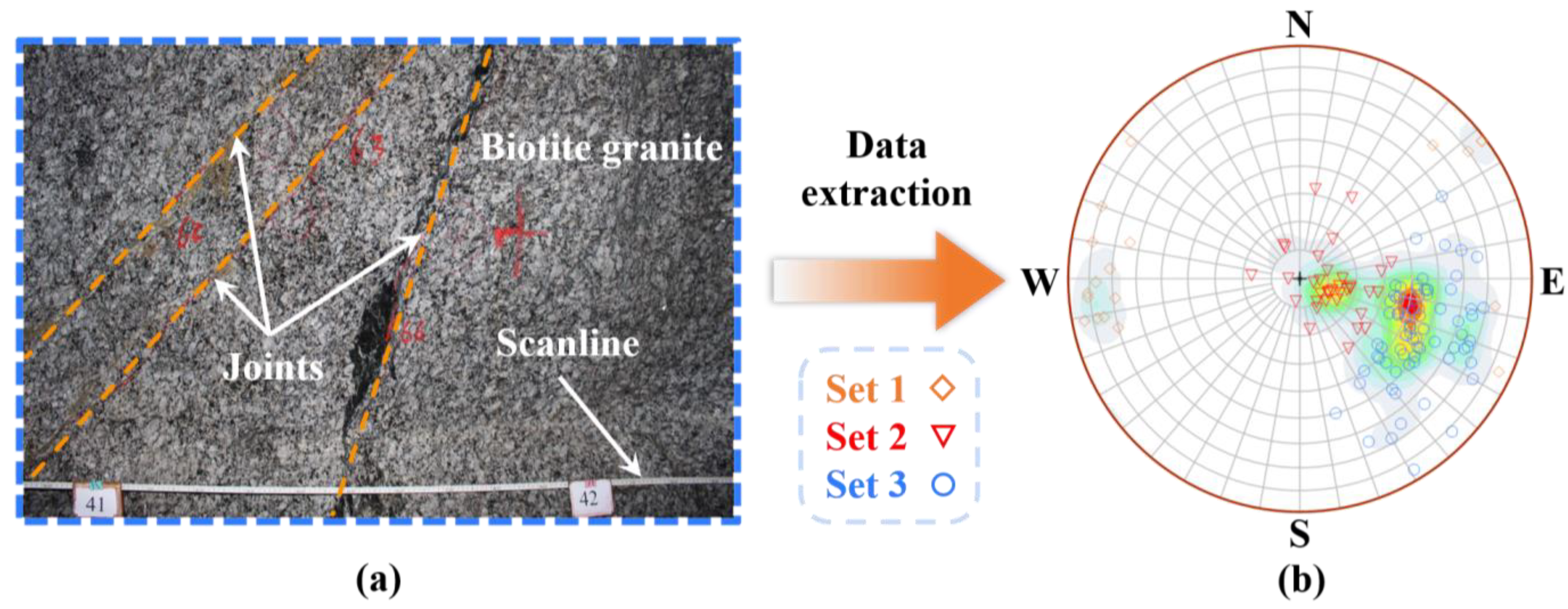
2.1. Joint Mapping

Joint mapping was conducted in an exploration tunnel with a length of 200 m and a radius of 2 m, which is located at the upper reaches of the Nu River, China. The lithology is primarily Cretaceous biotite granite, mainly consisting of quartz, plagioclase, potassium feldspar, and biotite. Cretaceous mafic intrusive rocks are also outcropped in this area, presenting as dykes with widths ranging from 0.05 to 5 m [32]. In this study, the window sampling method [5,33,34,35,36] was used for joint measurements: all joints intersecting the south-side wall of the exploration tunnel with a trace length larger than 0.5 m were mapped (Figure 1a). The measured data included the joint coordinate, orientation, trace length, spacing, and aperture. Based on the degrees of unloading and weathering, the investigated rock mass was divided into three zones: a strongly disturbed zone, weakly disturbed zone, and undisturbed zone. This study selected the 80 m-long undisturbed zone as the study region, where a total of 128 joints were measured [37]. The joints were grouped into three sets based on their orientations using the fuzzy K-means algorithm [38] (Figure 1b): (1) set 1 consists of steeply dipping joints with an average orientation of 265.0°∠82.2°; (2) set 2 consists of shallow-dipping joints with an average orientation of 100.6°∠11.8°; and (3) set 3 consists of moderately dipping joints with an average orientation of 113.3°∠48.3°.

2.2. Generation of the 3D DFN Model

The discrete fracture network DFN model can be an effective simulation tool as it can largely restore realistic discontinuity geometries for in situ applications [39,40]. Typically, the parameters used to generate the DFN model can be determined from a probability distribution function derived statistically based on in situ measurements. The 3D DFN model in this paper was established from our previous study. The detailed modeling procedures can refer to our previous work [35]. The statistical joint parameters used for the fracture network modelling are listed in Table 1. Joints are assumed to be disks and their spatial distributions are determined by three parameters [35]: (1) orientation, (2) diameter, and (3) location. The distribution of joint orientations in each joint set is described by an empirical probability distribution, with corrections applied to the relative frequency of each measured joint direction [34]. The size distribution of joints in each fracture set corresponds to their trace length distribution, which is statistically determined from the field data. The location of joint centers is assumed to follow a uniform Poisson distribution [1,5,36]. The stereological method [41] was used to determine the mean size of joints in each set according to their trace length distributions. The volume density λiV can be derived from the normal linear density λil of each joint set using the following formula [42,43]:
λ i V = 4 λ i l π E ( D 2 )
where E(D2) is the second moment of the joint diameter distribution. The number of joints ni in the simulated region for the i-th joint set is
n i = V λ i V
Finally, the Monte Carlo method was used to generate a 3D DFN model through the Poisson process in a 100 m × 60 m × 60 m simulated region, as shown in Figure 2. An artificial sampling window with the same size as the field measurement was set in the simulated rock mass to obtain joint parameters, including the number of joints, dip direction, dip angle, spherical standard deviation, and measured mean trace length and standard deviation. The DFN model was validated by comparing the parameters of the artificial joints with those obtained from field mapping. The results in Table 2 show that the simulated parameters agree well with the field measurements, indicating that the DFN model is reliable.

3. Calculation Method for Fluid Flow in Rock Masses

Fluid flow in fractured rock masses is typically assumed to follow the linear Darcy’s law [1,2], with the governing equation expressed as follows:
Q = A k μ Δ P Δ L
where Q is the total flow rate, A is the cross-sectional area, k is the permeability, μ is the fluid dynamic viscosity, ∆P is the pressure difference between the inlet and outlet boundaries, and ∆L is the seepage length.
For fluid flow in a fracture, it is often assumed that the both walls of the fracture are smooth, and the flow follows the cubic law [44]
q = h 3 12 μ Δ P Δ L
where q is the flow rate and h is the fracture aperture.

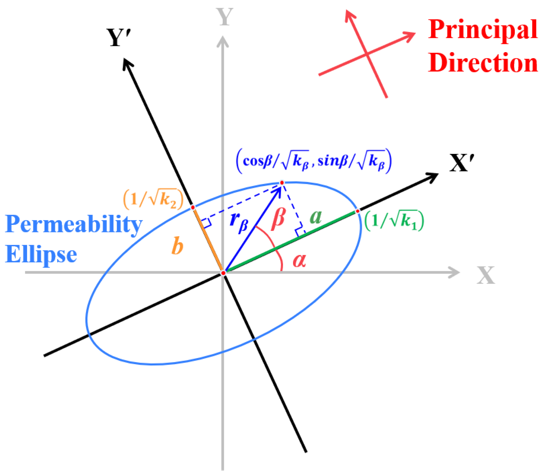
3.1. Permeability Tensor

The permeability of a fractured rock mass has tensor characteristics [16,26], which is a second-order positive definite tensor with six independent parameters:
k = k x x k x y k x z k y x k y y k y z k z x k z y k z z
where kxx, kyy, kzz, kxy, kxz, and kyz are the six independent components of the permeability tensor. The two-dimensional form is as follows:
k = k x x k x y k y x k y y
The permeability tensor has coordinated transformation characteristics, which are a function of the position coordinates and vary with the coordinate system. As shown in Figure 3, assuming that the local coordinate system xoy′ is formed by rotating the global coordinate system xoy counterclockwise by an angle α, the transformation relationship between them is expressed as follows:
k i j = k i j α i i α j j
where αxx = cosα, αxy = sinα, αyx = −sinα, and αyy = cosα. When the xoy coordinate system rotates counterclockwise to the xoy′ coordinate system, the transformation relationship between the elements of each matrix is described by
k x x k y y k x y = cos 2 α sin 2 α sin 2 α sin 2 α cos 2 α sin 2 α 1 2 sin 2 α 1 2 sin 2 α cos 2 α k x x k y y k x y
In the xoy′ coordinate system, assuming that the x′ and y′ axes are aligned with the principal permeability directions k1 and k2, the permeability in the direction obtained by rotating the x′ axis counterclockwise by an angle β is
k β = k 1 cos 2 β + k 2 sin 2 β
In the polar coordinate system, for a point with the polar angle β and radial distance rβ, which is assumed to be 1/kβ1/2 here, the projection of this point onto the Cartesian coordinate axes is (Figure 3)
x = cos β / k β y = sin β / k β
By transforming the above relationship into the Cartesian coordinate system, k1 and k2 satisfy the standard ellipse equation, which refers to the permeability ellipse [17]:
x 2 1 / k 1 2 + y 2 1 / k 2 2 = 1
The length of the two semi-axes of the ellipse is a = 1/k11/2 and b = 1/k21/2, and the radial distance rβ can be expressed numerically by the permeability in that direction rβ = 1/kβ1/2. The permeability ellipse is helpful for the visualization of the permeability tensor, which provides an effective way to evaluate the calculation results of the permeability.
Once the directional REV size is determined, the steady-state permeability of the fractured rock mass in different directions is calculated. In the polar coordinate system, the polar angle θ is defined as the counterclockwise angle from the x-axis direction to the fluid flow direction, and the polar radius r = 1/k1/2 is represented by the permeability. The models are rotated in 15° intervals to investigate the tensor characteristics of the directional permeability, resulting in 24 data points (θi, ri). The least square method is used to fit these points to an ellipse, yielding the fitting equation of the permeability ellipse and the six independent components of the permeability tensor. The eigenvalues and corresponding eigenvectors of the permeability tensor are then solved to obtain the principal permeabilities and their directions, respectively. To evaluate whether the fitting of the permeability ellipse could reasonably describe the permeability characteristics of the fractured rock mass, the fitting effectiveness is evaluated by the root mean square error (RMSNorm) [45]:
R M S Norm = 2 k 1 + k 2 1 N 1 N k t e n s o r ( θ ) k s i m ( θ ) 2
where N is the number of seepage directions, which is equal to 24 in this study; ktensor(θ) is the calculated permeability value in the θ direction; and ksim(θ) is the fitted permeability value in the θ direction. RMSNorm is a measure of the average difference between a statistical model’s predicted values and actual values. The smaller the RMSNorm, the smaller the difference between the calculated and fitted permeability values, indicating a better fit.

3.2. Fluid Flow Simulation Method

This study uses the commercial software package COMSOL Multiphysics 5.6 to simulate fluid flow in the fractured rock mass. Typically, the fluid velocity in the rock matrix is low, and its permeability is much smaller than that of fractures. Therefore, the Darcy’s law interface in the porous media and subsurface flow module is used to simulate fluid flow in a rock matrix. This interface is suitable for low-velocity flows or media with low permeability and porosity, driven by pressure gradients where frictional resistance in pores is the primary influencing factor on the flow. Combining Darcy’s law and the continuity equation yields the following generalized governing equation [17]:
t ρ ε p + ρ k μ p = Q m
where ρ is fluid density, εp is the porosity of rock matrix, and Qm is the mass source term.
For the calculation of fluid flow in fractures, the fracture flow interface based on the single fracture channel flow process is selected. The governing equation is derived by combining the generalized cubic law with the continuity equation [44]:
ρ q f = d f Q m
q f = d f 3 12 μ f f p
where qf is the volume flow rate per unit length in the fracture, df is the aperture or fracture thickness, and ff is the roughness factor.
The above calculation method ensures the momentum and mass conservation in the process of seepage calculation. The continuity boundary conditions also ensure the continuity of pressure and mass flux. The fluid distribution in fractures is coupled with the rock matrix through the exchange of the flow and pressure between the upper and lower surfaces of the fractures. Changes in the fluid density and fracture aperture caused by variations in temperature and stress are not considered, and the fluid is assumed to be an incompressible medium under steady laminar flow driven only by the pressure head. These assumptions improve the computational efficiency and ensure the accuracy of the hydraulic property estimation.

3.3. Verification

In order to validate the numerical method, a series of simple fracture models, including nine single-fracture models and one double-fracture model, were selected, as shown in Figure 4. In the single fracture models, the angle α between the fracture and the horizontal direction varies from 50° to 90°, and the aperture is 5 mm. In the double-fracture model, the apertures of two fractures are 4 mm and 5 mm, respectively. The model sides are 20 m × 20 m. With head H2 = 30 m applied above the model and head H1 = 10 m below, the head varies linearly on both sides of the boundary. The steady-state fluid flow simulation was performed using the numerical method and the simulation results were then compared with those calculated by the theoretical method [44] and the modified equivalent permeability model proposed by Wang et al. [46]. Table 3 shows the simulation results of the flow rate at the outlet for the fracture models obtained by different methods. The results show that the relative difference between the simulation results of this work and the results obtained by the two previous methods are all below 5%, indicating that the numerical method performs well in simulating fluid flows in fractured rock masses.

4. Numerical Simulation

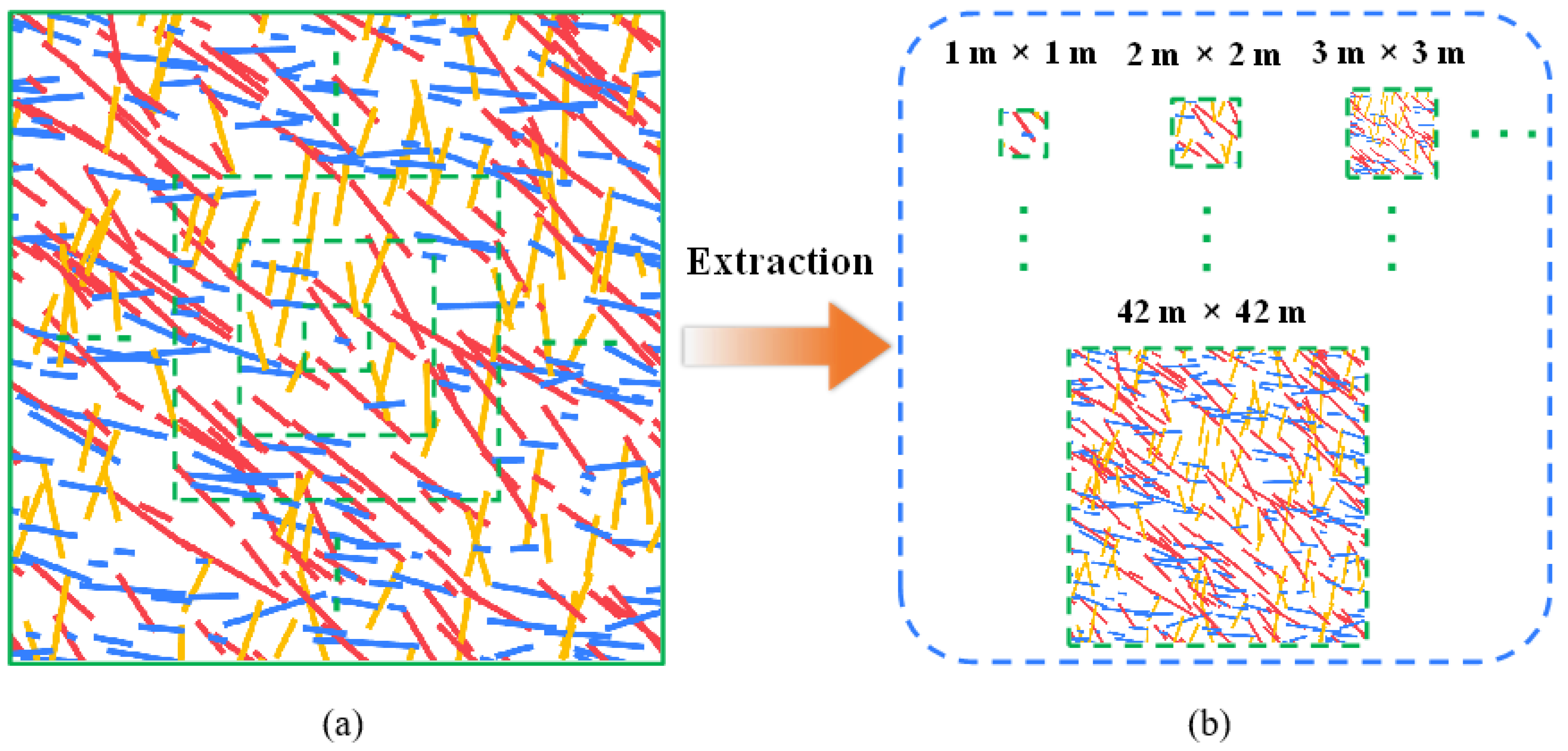
4.1. Model Generation and Boundary Conditions

A 60 m × 60 m 2D DFN model was extracted from the 3D DFN model at x = 50 m along a plane perpendicular to the x-axis, serving as the ’master’ model. A series of square sub-models with side lengths varying from 1 m to 42 m with 1 m increments (i.e., 1 m, 2 m, 3 m, …, 42 m) were then extracted from the ’master’ model, as shown in Figure 5. In addition, each of the sub-models was rotated in a counterclockwise direction at 15° intervals with the rotation angle θ (θ = 0°, 15°, 30°, 45°, 60°, 75°, 90°, 105°, 120°, 135°, 150°, and 165°), which was defined as the angle between the fluid flow direction and the x-axis direction, as shown in Figure 6. All sub-models were imported into the software COMSOL Multiphysics to study the variation in the equivalent permeability with the model size and the directional permeability. Thus, 504 numerical simulations were performed. The boundary conditions imposed on the models are shown in Figure 7. The two lateral boundaries are constant pressure boundaries, where a 0.1 MPa/m pressure is applied to the left side and a 0.5 MPa/m pressure is applied to on the right side, yielding a constant pressure differential of 0.4 MPa/m in the flow direction. The top and bottom boundaries are impermeable boundaries.

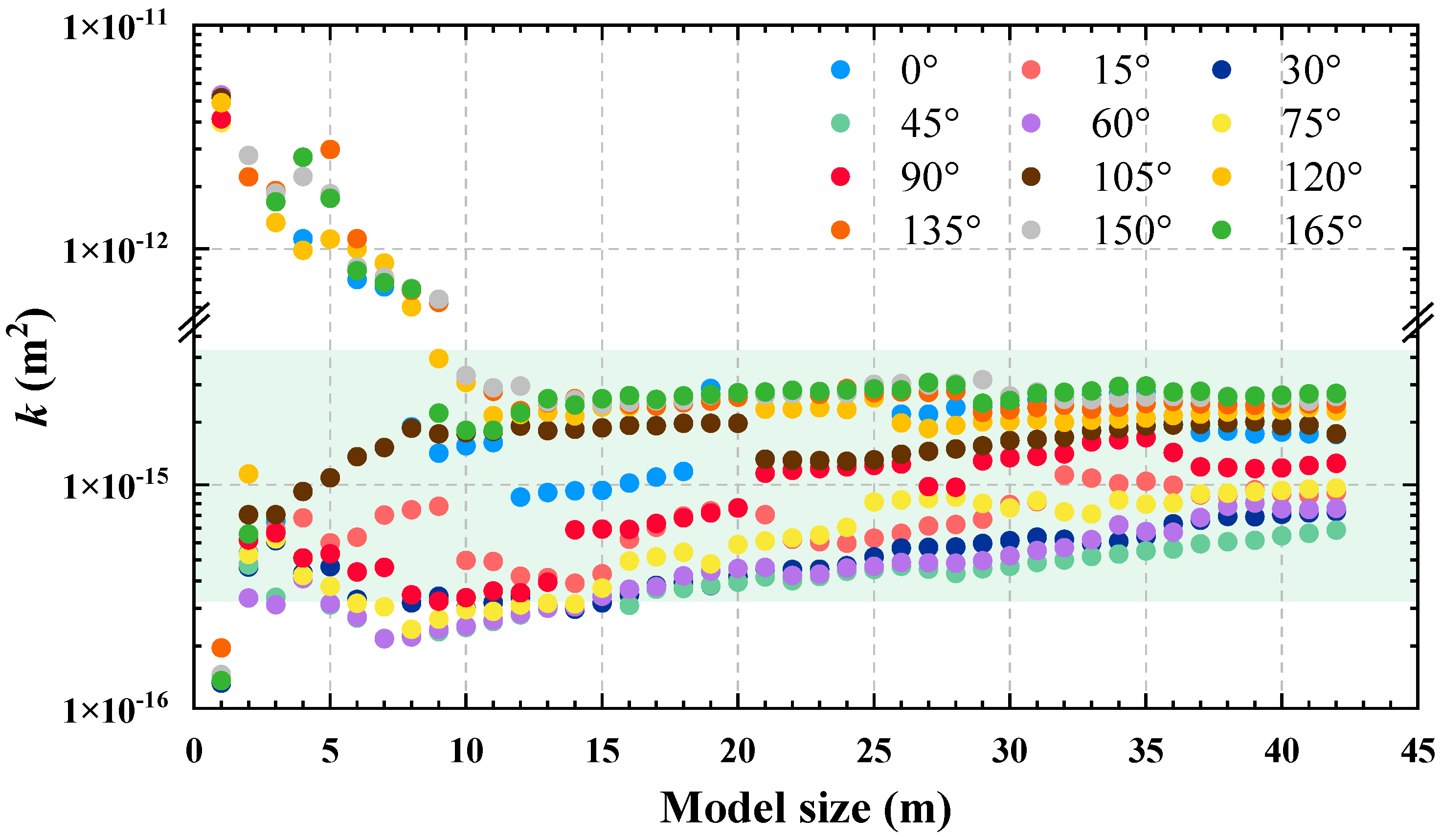
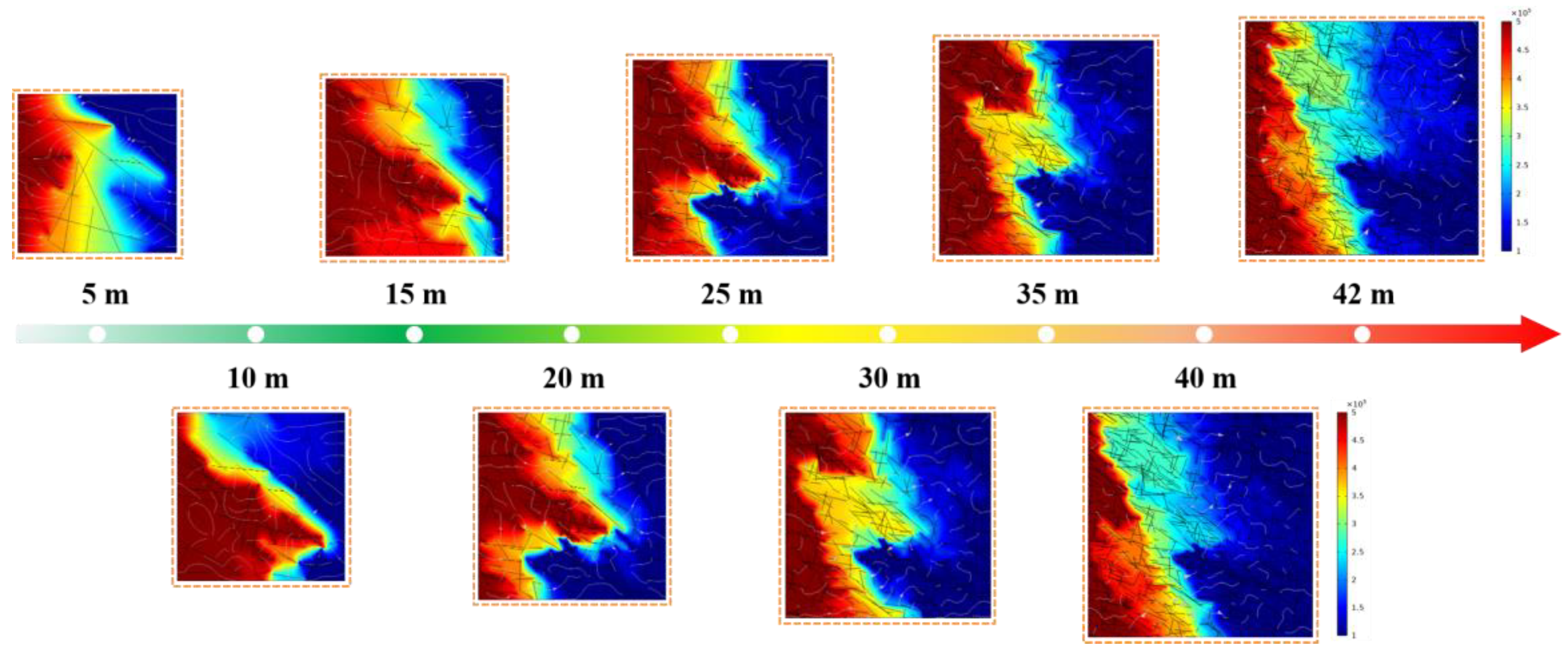
4.2. Simulation Results

Figure 8 shows the variation in the equivalent permeability k with the model size in different fluid flow directions. When the model size increases from 1 m to 11 m, the value of k fluctuates drastically due to the existence of persistent joints in the models. As the model size further increases, the value of k begins to converge to a constant due to the absence of persistent joints. The plots in Figure 8 also indicate that the permeability of the rock mass presents strong anisotropy. This anisotropy decreases with increasing model sizes and eventually stabilizes. Figure 9 gives an example of the fluid pressure distribution in the models when θ is 0°. It seems that the permeability of the small-sized models is typically dominated by a highly permeable long persistent joint.

5. Estimation of the REV Size

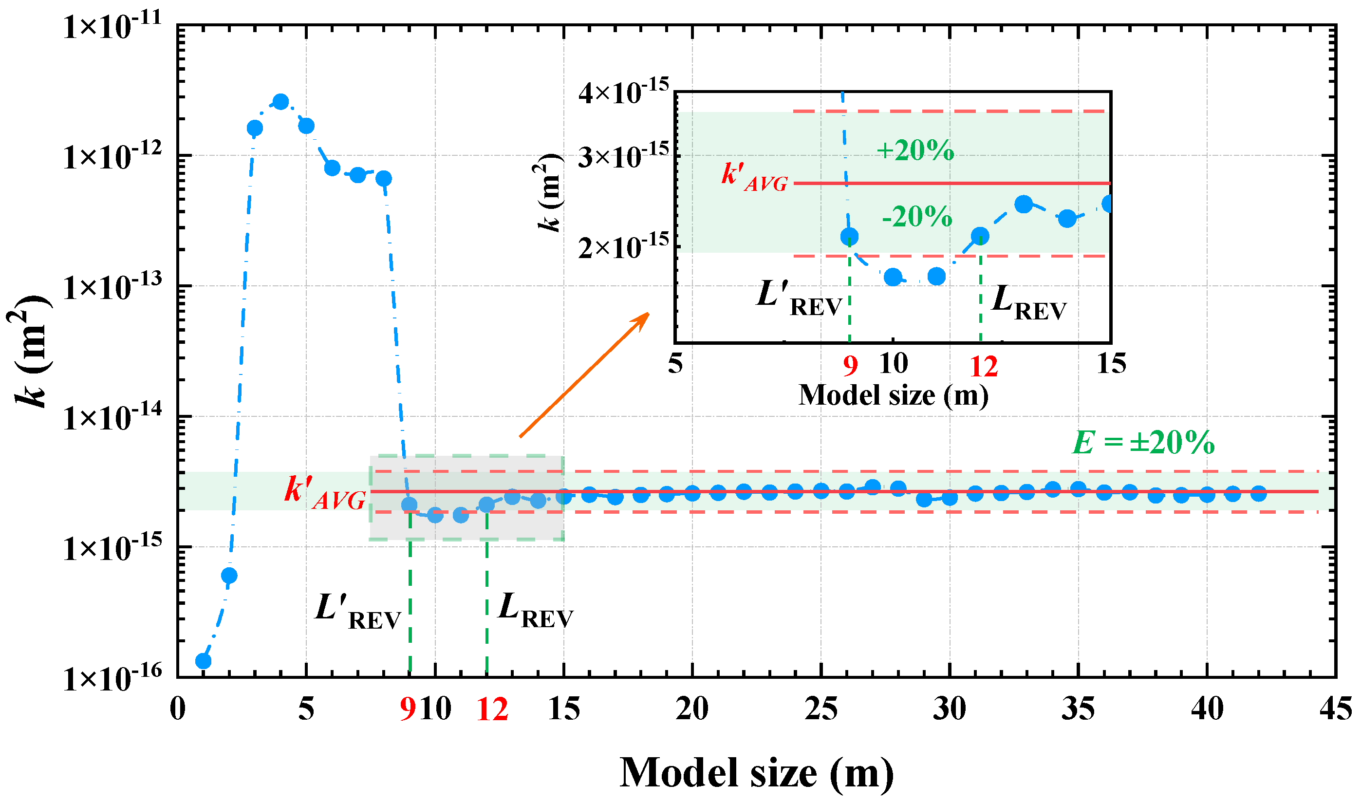
5.1. Estimation of the REV Size Based on Permeability

The REV is defined as the smallest element that can represent the macroscopic properties of a fractured rock mass [17,18,19]. The permeability of a rock mass shows a constant characteristic when its size is larger than the REV size. Once the rock mass size exceeds LREV, its permeability presents both constant and tensor properties [16,44]. This study used the coefficient of variation (CV), defined as the ratio of the standard deviation to the mean, to quantitatively determine the REV size. CV has been widely used to determine the REV size of rock masses based on mechanical parameters [27,28]. Generally, when the calculated CV value is less than 0.2, the sample size is considered the REV size [45]. This study gives the estimated results of the REV size considering different threshold values of CV (i.e., CV = 0.2, 0.19, 0.18, 0.17, 0.16, 0.15, 0.14, 0.13, 0.12, 0.11, and 0.1). In this research, the REV size determined by CV refers to LREV, and the average permeability of the rock mass larger than the REV size refers to kAVG. Since CV only reflects the cumulative error of measured data but cannot measure their local fluctuations, we used the following method to correct the REV size: the minimum size corresponding to the permeability k within a 20% fluctuation range of kAVG was taken as the REV size and denoted as LREV (Figure 10), and the average permeability for the models with sizes larger than LREV was calculated as the equivalent permeability kAVG.
The equivalent permeability kAVG in different flow directions was plotted in the polar coordinate system to fit the permeability ellipse. The fitting of the permeability ellipse was evaluated by calculating the root mean square error (RMSNorm). A small RMSNorm value means that the deviation between the original values and fitted values is small. It is generally considered that the fitting of the permeability ellipse is satisfying when the value of RMSNorm is less than 0.2 [2,5,14,45]. The LREV values determined by permeability according to different threshold values of CV are shown in Table 4. By limiting the fluctuation range of the permeability within a 20% fluctuation range of kAVG, the LREV values were obtained (Table 5). The LREV, kAVG, and fitted permeability ellipse in each seepage direction were plotted in the polar coordinate system (Figure 11). The results show that the values of LREV in the flow direction with θ = 0–105° are significantly larger than those in the flow direction with θ = 120–165°. The difference in the kAVG values and permeability ellipses obtained by the different CV values are not significant, but CV does affect the determination of LREV, especially in the seepage directions where the LREV values are relatively large. Figure 12 shows the values of RMSNorm for the fitting of the permeability ellipse under different threshold values of CV. All calculated results are less than 0.2, indicating that the fit is good. The values of RMSNorm achieve the minimum value of 0.0617 when the CV = 0.18, suggesting that the fit of the permeability ellipse is the best. Therefore, CV = 0.18 is adopted in this study as the threshold value for determining the REV size.
Figure 13a shows that the REV size is smallest (LREV = 6 m) in the seepage direction of θ = 105°, which is 3–4 times the mean joint trace length. Additionally, the REV size is the largest (LREV = 36 m) for θ = 0° and 90°. In the seepage directions of θ = 0–90°, the value of LREV is no less than 20 m, whereas the value of LREV does not exceed 12 m in the seepage directions of θ = 105–165°. Due to the influence of the joints, the rock mass permeability exhibits strong anisotropy, with the value of k ranging from 4.71 × 10⁻¹⁶ to 2.55 × 10⁻¹⁵ m2 (Figure 13b). The long and short principal axes of the permeability ellipse are at θ = 48° and θ = 138°, respectively (Figure 13c). Figure 13 also shows that the rock mass permeability is relatively smaller and the REV size is relatively larger in the seepage directions of θ = 0–90° compared with the seepage directions of θ = 105–165°. Therefore, it seems that the directional REV size is negatively correlated with the directional permeability of the rock mass.

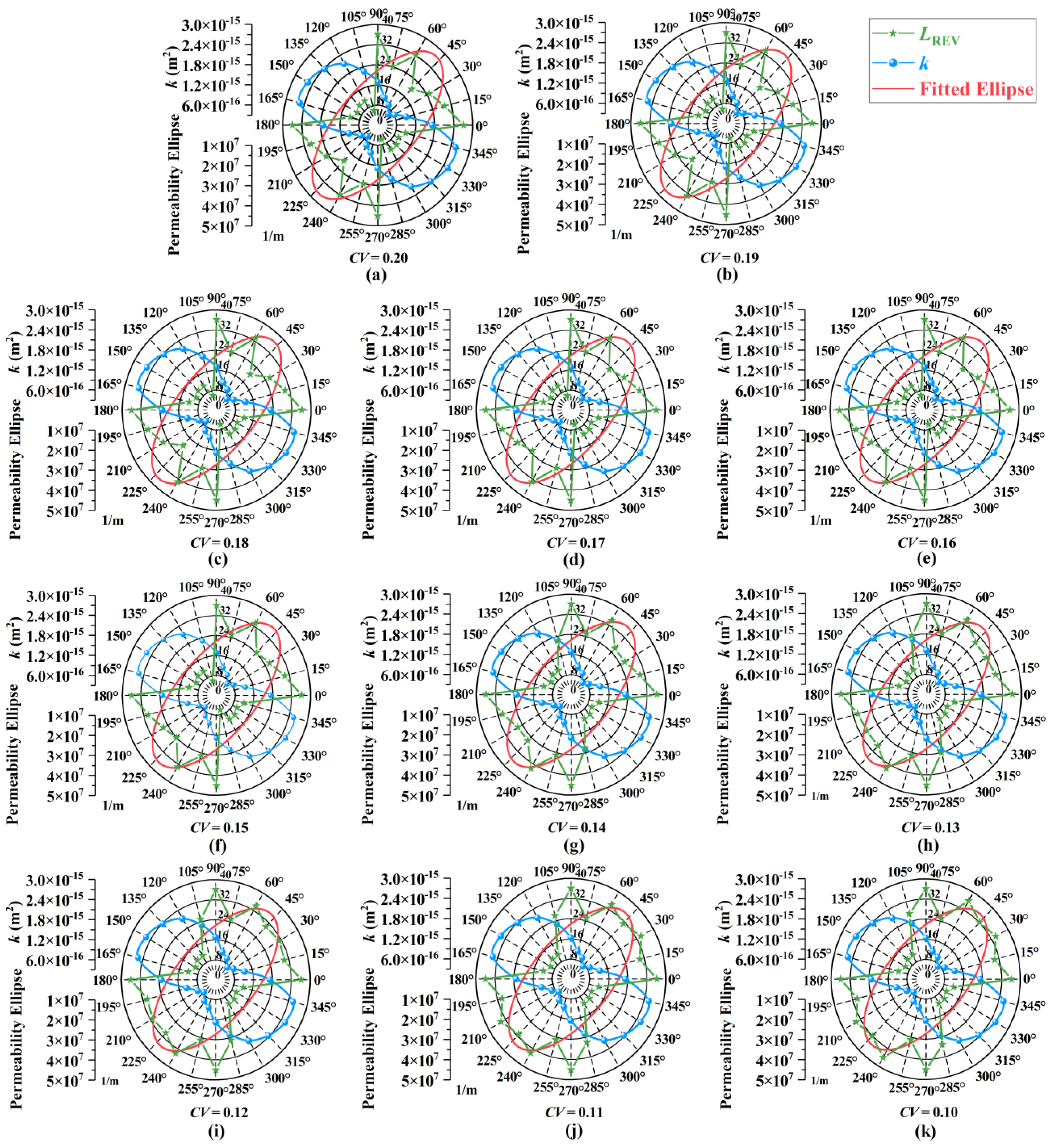
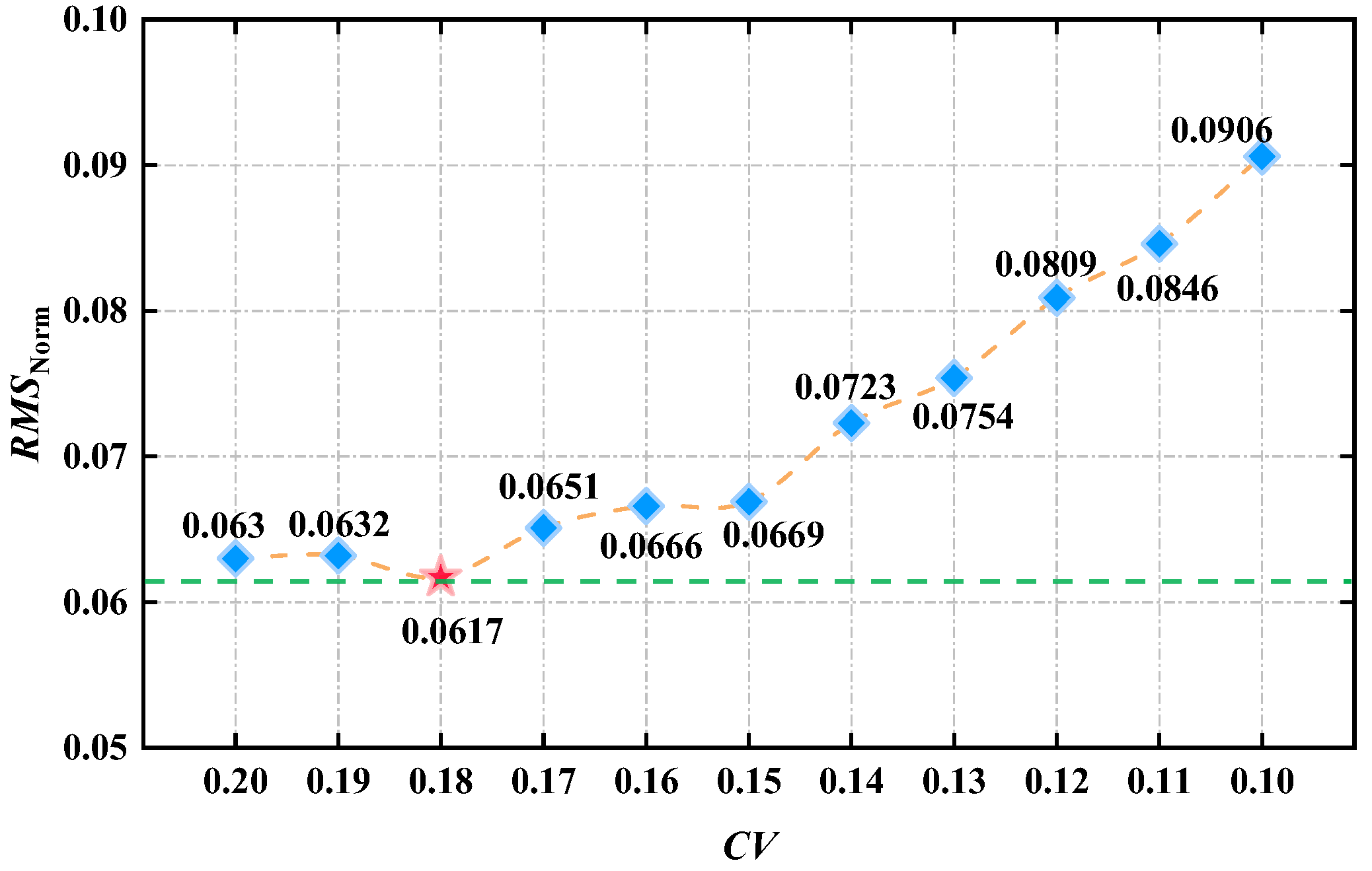
5.2. Estimation of the REV Size Based on the Anisotropy Index

The anisotropy index (AIp) was introduced to quantitatively describe the anisotropy of the permeability of the fractured rock mass:
A I p = k max k min
where kmax and kmin represent the maximum and minimum permeability values in different directions.
Figure 14 shows the variation in the AIp with the model size. When the model size reaches 11 m, the AIp value drops by nearly three orders of magnitude. Beyond this size, the AIp values remain below 10, indicating a dramatic change in permeability. To verify the applicability of the AIp for estimating the REV size, the RMSNorm was used for comparison (Figure 14). The RMSNorm is less than 0.2 when the size of the rock mass reaches 11 m, which is consistent with the REV size determined by the AIp. Figure 15 shows the variation in the permeability k with the model size. The average permeability kAVG reaches the minimum value of 4.71 × 10⁻¹⁶ m2 at θ = 45° and it reaches the maximum value of 2.55 × 10⁻¹⁵ m2 at θ = 150°. The permeability exhibits a variation pattern similar to a cosine function with a periodicity of π, reflecting the directional properties of the directional permeability.

6. Discussion

6.1. Influence of the Joint Geometry on the Permeability and REV Size

The statistical parameters of the joints in the 2D ‘master’ DFN model (Figure 5a) are shown in Figure 16. Here, the orientation of a joint in a 2D plane is defined as the counterclockwise angle from the x-axis direction to the joint trace. Based on this definition, the average orientation of the joint sets S1, S2, and S3 is 80.5°, 137.5°, and 171.9°, respectively. Notably, the LREV values at θ = 90°, 135°, and 180° are 36 m, 11 m, and 36 m, respectively, which are all the local maxima. Meanwhile, the bisector angles of each pair of the joint sets (i.e., S1 and S3, S1 and S2, and S2 and S3) are 36.2°, 109.1°, and 154.8°, respectively, while the LREV values at θ = 45°, 105°, and 150° are 20 m, 6 m, and 10 m, respectively, which are all the local minima. Therefore, it could be concluded that the local maximum REV size appears in the direction of the average orientation of each joint set, while the local minimum REV size appears in the direction of the angle bisector of the average angle between each pair of the joint sets. We also find that the smallest value of LREV (6 m) appears in the angle bisector direction between the joint sets S1 and S2 with larger joint lengths, whereas the largest value of LREV (36 m) appears in the average orientation direction of the joint set S3 with a smaller joint length. This indicates that a larger joint length leads to a smaller value of LREV. The fracture groups with larger average trace lengths are easier to intersect with the fractures distributed in other directions, which in turn form more persistent joints along that direction, greatly facilitating the connectivity of the fracture network. As the model size increases, the seepage process in this direction will reach the steady state more quickly, thus making the REV size smaller than the other directions.

6.2. Comparison Between the Geometric and Hydraulic REV Sizes

The geometric parameters are also important indicators for determining the REV size of rock masses. This study used the geometric parameters (i.e., joint connectivity and intensity) to estimate the geometric REV size. Joint connectivity refers to the number of joint intersections per unit area, while the joint intensity here refers to the number of joints per unit area (P20) and the total joint length per unit area (P21) [47]. The coefficient of variation (CV) was used to determine the geometric REV size. A CV value of 0.05 was selected as the threshold value for the REV size estimation.
The variation in the geometric parameters of the fractured rock mass with model size is shown in Figure 17. When the model sizes are 20 m, 10 m, and 7 m, the CV values for joint connectivity, P20, and P21 are all less than 0.05. Therefore, the geometric REV sizes based on joint connectivity, P20, and P21 are 20 m, 10 m, and 7 m, respectively. This observation reveals an interesting phenomenon: (1) the geometric REV size estimated by joint connectivity (20 m) is approximately equal to the lower limit of the REV size in the directions with relatively low permeability (i.e., θ = 0°, 15°, 30°, 45°, 60°, 75°, and 90°); (2) the geometric REV size estimated by P21 (7 m) is similar to the lower limit of the REV size in the directions with relatively high permeability (i.e., θ = 105°, 120°, 135°, 150°, and 165°); and (3) the geometric REV size estimated by P20 (10 m) is approximately equal to the REV size determined by the AIp. In fact, the hydraulic properties of a rock mass are influenced by various joint parameters, such as the joint density, length, aperture, orientation, etc. The REV size based on geometric parameters could not reflect the variation and anisotropy of hydraulic properties, leading to incorrect characterization and property upscaling.
Fractured rock masses, due to their complex internal structures, often exhibit significant hydraulic anisotropy, making the variation in REV size in different directions non-negligible. Traditional homogeneous assumptions or isotropic models fail to accurately describe the permeability characteristics of fractured rock masses in many cases, leading to considerable deviations in seepage analysis and engineering calculations. The newly proposed permeability-based method for estimating the directional REV size of fractured rock masses provides a more targeted approach for characterizing rock mass permeability. In dam design, accurately assessing the permeability of the bedrock has profound implications for the design of anti-seepage systems, the development of seepage monitoring plans, and the prediction of long-term operational safety. Therefore, a reasonable estimation of the REV size of fractured rock masses, especially the directional REV size under anisotropic conditions, is crucial for improving the accuracy of permeability predictions, optimizing seepage control measures, and enhancing dam safety assessments.
However, for real natural fractured rock masses, further research is needed. First, two-dimensional models inherently underestimate the connectivity and anisotropy of three-dimensional fracture networks. As a result, the 2D approach may lead to an underestimation of permeability, thereby affecting the estimation of the REV size. This limitation is particularly evident in rock masses with significant variations in fracture dip angles or high fracture densities. Second, the geometric shape and surface roughness of fractures influence the fluid distribution, leading to channeling and anomalous transport phenomena, which in turn affect permeability predictions. Therefore, although this study provides an effective 2D method for estimating the directional REV size of fractured rock masses, further refinements are necessary for application to real natural fractured rock masses. Future research could integrate three-dimensional DFN models, fracture roughness models, and a geometric morphological analysis to explore how these factors interact with fracture network connectivity, thereby improving the accuracy and reliability of directional REV assessments.

7. Conclusions

This paper investigates the scale dependency and anisotropy of the hydraulic properties of a fractured rock mass. A 3D DFN model was built using the joint data obtained from a dam site in southwest China. A total of 504 2D sub-models with sizes ranging from 1 m × 1 m to 42 m × 42 m were extracted from the DFN model and then were used for equivalent permeability tensor calculations based on the finite element method. We proposed a new method for estimating the directional REV size of fractured rock masses based on permeability. The steady-state average permeability in each direction was calculated and the permeability ellipse was fitted.
The results show that the rock mass permeability exhibits strong anisotropy, with the value of k ranging from 4.71 × 10⁻¹⁶ to 2.55 × 10⁻¹⁵ m2. The long and short principal axes of the fitted permeability ellipse are θ = 48° and θ = 138°, respectively. The hydraulic REV size LREV is smallest (6 m) in the seepage direction of θ = 105°, which is 3–4 times the mean joint trace length. Additionally, the REV size is the largest (LREV = 36 m) when θ = 0° and 90°. We also find that the smallest value of LREV (6 m) appears in the bisector direction between the joint sets S1 and S2 with larger joint lengths, whereas the largest value of LREV (36 m) appears in the average orientation direction of the joint set S3 with a smaller joint length. This indicates that a larger joint length leads to a smaller value of LREV. A comparison between the geometric and hydraulic REV indicates that the geometric REV size falls into the range of the hydraulic REV size.
However, the 2D model used in this research inevitably underestimates the connectivity and permeability of the realistic 3D fracture network system [1,48,49,50]. Moreover, aperture changes induced by stress variations are not within the scope of this work. Future research is recommended to utilize a 3D DFN model considering aperture changes to study fluid flow in fractured rock masses.

Author Contributions

Conceptualization, H.Q. and Y.L.; methodology, H.Q.; software, H.Q.; formal analysis, H.Q.; investigation, H.Q. and Y.L.; data curation, H.Q. and Y.L.; writing—original draft preparation, H.Q. and Y.L.; writing—review and editing, H.Q. and Y.L. All authors have read and agreed to the published version of the manuscript.

Funding

This research was funded by the National Natural Science Foundation of China (NSFC) (No. 42077258).

Data Availability Statement

The data are available from the corresponding author upon reasonable request.

Acknowledgments

Thanks to the editor and the anonymous reviewers for their constructive comments and suggestions for improving the quality of this paper.

Conflicts of Interest

The authors declare that they have no known competing financial interests or personal relationships that could have appeared to influence the work reported in this paper.

References

  1. Min, K.-B.; Jing, L.; Stephansson, O. Determining the Equivalent Permeability Tensor for Fractured Rock Masses Using a Stochastic REV Approach: Method and Application to the Field Data from Sellafield, UK. Hydrogeol. J. 2004, 12, 497–510. [Google Scholar] [CrossRef]
  2. Baghbanan, A.; Jing, L. Hydraulic Properties of Fractured Rock Masses with Correlated Fracture Length and Aperture. Int. J. Rock Mech. Min. Sci. 2007, 44, 704–719. [Google Scholar] [CrossRef]
  3. Cui, Z.; Zhang, Y.; Sheng, Q.; Cui, L. Investigating the Scale Effect of Rock Mass in the Yangfanggou Hydropower Plant with the Discrete Fracture Network Engineering Approach. Int. J. Geomech. 2020, 20, 04020033. [Google Scholar] [CrossRef]
  4. Luo, L.; Liang, X.; Ma, B.; Zhou, H. A Karst Networks Generation Model Based on the Anisotropic Fast Marching Algorithm. J. Hydrol. 2021, 600, 126507. [Google Scholar] [CrossRef]
  5. Yu, L.; Zhang, J.; Liu, R.; Li, S.; Liu, D.; Wang, X. Estimation of the Representative Elementary Volume of Three-Dimensional Fracture Networks Based on Permeability and Trace Map Analysis: A Case Study. Eng. Geol. 2022, 309, 106848. [Google Scholar] [CrossRef]
  6. Rong, G.; Peng, J.; Wang, X.; Liu, G.; Hou, D. Permeability Tensor and Representative Elementary Volume of Fractured Rock Masses. Hydrogeol. J. 2013, 21, 1655–1671. [Google Scholar] [CrossRef]
  7. Liu, R.; Zhu, T.; Jiang, Y.; Li, B.; Yu, L.; Du, Y.; Wang, Y. A Predictive Model Correlating Permeability to Two-Dimensional Fracture Network Parameters. Bull. Eng. Geol. Environ. 2019, 78, 1589–1605. [Google Scholar] [CrossRef]
  8. Oda, M. A Method for Evaluating the Effect of Crack Geometry on the Mechanical Behavior of Cracked Rock Masses. Mech. Mater. 1983, 2, 163–171. [Google Scholar] [CrossRef]
  9. Park, B.; Min, K.-B. Bonded-Particle Discrete Element Modeling of Mechanical Behavior of Transversely Isotropic Rock. Int. J. Rock Mech. Min. Sci. 2015, 76, 243–255. [Google Scholar] [CrossRef]
  10. Wu, Q.; Jiang, Y.; Tang, H.; Luo, H.; Wang, X.; Kang, J.; Zhang, S.; Yi, X.; Fan, L. Experimental and Numerical Studies on the Evolution of Shear Behaviour and Damage of Natural Discontinuities at the Interface Between Different Rock Types. Rock Mech. Rock Eng. 2020, 53, 3721–3744. [Google Scholar] [CrossRef]
  11. Wu, Q.; Kulatilake, P.H.S.W. REV and Its Properties on Fracture System and Mechanical Properties, and an Orthotropic Constitutive Model for a Jointed Rock Mass in a Dam Site in China. Comput. Geotech. 2012, 43, 124–142. [Google Scholar] [CrossRef]
  12. Khani, A.; Baghbanan, A.; Hashemolhosseini, H. Numerical Investigation of the Effect of Fracture Intensity on Deformability and REV of Fractured Rock Masses. Int. J. Rock Mech. Min. Sci. 2013, 63, 104–112. [Google Scholar] [CrossRef]
  13. He, J.; Chen, S.; Shahrour, I. Numerical Estimation and Prediction of Stress-Dependent Permeability Tensor for Fractured Rock Masses. Int. J. Rock Mech. Min. Sci. 2013, 59, 70–79. [Google Scholar] [CrossRef]
  14. Li, Z.-W.; Feng, X.-T.; Zhang, Y.-J.; Xu, T.-F. Effect of Hydrological Spatial Variability on the Heat Production Performance of a Naturally Fractured Geothermal Reservoir. Environ. Earth Sci. 2018, 77, 496. [Google Scholar] [CrossRef]
  15. Mahboubi Niazmandi, M.; Binesh, S.M. A DFN–DEM Approach to Study the Influence of Confinement on the REV Size of Fractured Rock Masses. Iran. J. Sci. Technol. Trans. Civ. Eng. 2020, 44, 587–601. [Google Scholar] [CrossRef]
  16. Long, J.C.S.; Remer, J.S.; Wilson, C.R.; Witherspoon, P.A. Porous Media Equivalents for Networks of Discontinuous Fractures. Water Resour. Res. 1982, 18, 645–658. [Google Scholar] [CrossRef]
  17. Bear, J. Dynamics of Fluids in Porous Media; Elsevier: New York, NY, USA, 1972. [Google Scholar]
  18. Oda, M. A Method for Evaluating the Representative Elementary Volume Based on Joint Survey of Rock Masses. Can. Geotech. J. 1988, 25, 440–447. [Google Scholar] [CrossRef]
  19. Esmaieli, K.; Hadjigeorgiou, J.; Grenon, M. Estimating Geometrical and Mechanical REV Based on Synthetic Rock Mass Models at Brunswick Mine. Int. J. Rock Mech. Min. Sci. 2010, 47, 915–926. [Google Scholar] [CrossRef]
  20. Wei, L.; Hudson, J.A. A Coupled Discrete-Continuum Approach for Modelling of Water Flow in Jointed Rocks. Géotechnique 1993, 43, 21–36. [Google Scholar] [CrossRef]
  21. Gutierrez, M.; Youn, D.-J. Effects of Fracture Distribution and Length Scale on the Equivalent Continuum Elastic Compliance of Fractured Rock Masses. J. Rock Mech. Geotech. Eng. 2015, 7, 626–637. [Google Scholar] [CrossRef]
  22. Ni, P.; Wang, S.; Wang, C.; Zhang, S. Estimation of REV Size for Fractured Rock Mass Based on Damage Coefficient. Rock Mech. Rock Eng. 2017, 50, 555–570. [Google Scholar] [CrossRef]
  23. Li, Y.; Chen, J.; Shang, Y. Determination of the Geometrical REV Based on Fracture Connectivity: A Case Study of an Underground Excavation at the Songta Dam Site, China. Bull. Eng. Geol. Environ. 2018, 77, 1599–1606. [Google Scholar] [CrossRef]
  24. Schultz, R.A. Relative Scale and the Strength and Deformability of Rock Masses. J. Struct. Geol. 1996, 18, 1139–1149. [Google Scholar] [CrossRef]
  25. Zhang, G.; Xu, W. Analysis of Joint Network Simulation Method and REV Scale. Rock Soil. Mech. 2008, 29, 1675–1680. [Google Scholar]
  26. Min, K.-B.; Jing, L. Numerical Determination of the Equivalent Elastic Compliance Tensor for Fractured Rock Masses Using the Distinct Element Method. Int. J. Rock Mech. Min. Sci. 2003, 40, 795–816. [Google Scholar] [CrossRef]
  27. Huang, H.; Shen, J.; Chen, Q.; Karakus, M. Estimation of REV for Fractured Rock Masses Based on Geological Strength Index. Int. J. Rock Mech. Min. Sci. 2020, 126, 104179. [Google Scholar] [CrossRef]
  28. Li, Y.; Wang, R.; Chen, J.; Zhang, Z.; Li, K.; Han, X. Scale Dependency and Anisotropy of Mechanical Properties of Jointed Rock Masses: Insights from a Numerical Study. Bull. Eng. Geol. Environ. 2023, 82, 114. [Google Scholar] [CrossRef]
  29. Wang, P.; Ren, F.; Miao, S.; Cai, M.; Yang, T. Evaluation of the Anisotropy and Directionality of a Jointed Rock Mass under Numerical Direct Shear Tests. Eng. Geol. 2017, 225, 29–41. [Google Scholar] [CrossRef]
  30. Bang, S.-H.; Jeon, S.-W.; Kwon, S.-K. Modeling the Hydraulic Characteristics of a Fractured Rock Mass with Correlated Fracture Length and Aperture: Application in the Underground Research Tunnel at Kaeri. Nucl. Eng. Technol. 2012, 44, 639–652. [Google Scholar] [CrossRef]
  31. Wang, Z.; Li, W.; Qiao, L.; Liu, J.; Yang, J. Hydraulic Properties of Fractured Rock Mass with Correlated Fracture Length and Aperture in Both Radial and Unidirectional Flow Configurations. Comput. Geotech. 2018, 104, 167–184. [Google Scholar] [CrossRef]
  32. Li, Y.; Wang, Q.; Chen, J.; Han, L.; Song, S. Identification of Structural Domain Boundaries at the Songta Dam Site Based on Nonparametric Tests. Int. J. Rock Mech. Min. Sci. 2014, 70, 177–184. [Google Scholar] [CrossRef]
  33. Mauldon, M.; Dunne, W.M.; Rohrbaugh, M.B. Circular Scanlines and Circular Windows: New Tools for Characterizing the Geometry of Fracture Traces. J. Struct. Geol. 2001, 23, 247–258. [Google Scholar] [CrossRef]
  34. Wu, Q.; Kulatilake, P.H.S.W.; Tang, H. Comparison of Rock Discontinuity Mean Trace Length and Density Estimation Methods Using Discontinuity Data from an Outcrop in Wenchuan Area, China. Comput. Geotech. 2011, 38, 258–268. [Google Scholar] [CrossRef]
  35. Han, X.; Chen, J.; Wang, Q.; Li, Y.; Zhang, W.; Yu, T. A 3D Fracture Network Model for the Undisturbed Rock Mass at the Songta Dam Site Based on Small Samples. Rock Mech. Rock Eng. 2016, 49, 611–619. [Google Scholar] [CrossRef]
  36. Xu, W.; Zhang, Y.; Li, X.; Wang, X.; Ma, F.; Zhao, J.; Zhang, Y. Extraction and Statistics of Discontinuity Orientation and Trace Length from Typical Fractured Rock Mass: A Case Study of the Xinchang Underground Research Laboratory Site, China. Eng. Geol. 2020, 269, 105553. [Google Scholar] [CrossRef]
  37. Li, Y.; Chen, J.; Shang, Y. Connectivity of Three-Dimensional Fracture Networks: A Case Study from a Dam Site in Southwest China. Rock Mech. Rock Eng. 2017, 50, 241–249. [Google Scholar] [CrossRef]
  38. Hammah, R.E.; Curran, J.H. On Distance Measures for the Fuzzy K-Means Algorithm for Joint Data. Rock Mech. Rock Eng. 1999, 32, 1–27. [Google Scholar] [CrossRef]
  39. Qiu, J.; Zhou, C.; Wang, Z.; Feng, F. Dynamic Responses and Failure Behavior of Jointed Rock Masses Considering Pre-Existing Joints Using a Hybrid BPM-DFN Approach. Comput. Geotech. 2023, 155, 105237. [Google Scholar] [CrossRef]
  40. Zhou, C.; Xie, H.; Zhu, J. Revealing Size Effect and Associated Variability of Rocks Based on BPM–μDFN Modelling: Significance of Internal Microstructure and Strain Rate. Rock Mech. Rock Eng. 2024, 57, 2983–2996. [Google Scholar] [CrossRef]
  41. Warburton, P.M. A Stereological Interpretation of Joint Trace Data. Int. J. Rock Mech. Min. Sci. Geomech. Abstr. 1980, 17, 181–190. [Google Scholar] [CrossRef]
  42. Oda, M. Fabric Tensor for Discontinuous Geological Materials. Soils Found. 1982, 22, 96–108. [Google Scholar] [CrossRef]
  43. Kulatilake, P.H.S.W.; Wathugala, D.N.; Stephansson, O. Stochastic Three Dimensional Joint Size, Intensity and System Modelling and a Validation to an Area in Stripa Mine, Sweden. Soils Found. 1993, 33, 55–70. [Google Scholar] [CrossRef]
  44. Snow, D.T. Anisotropic Permeability of Fractured Media. Water Resour. Res. 1969, 5, 1273–1289. [Google Scholar] [CrossRef]
  45. Öhman, J.; Niemi, A. Upscaling of Fracture Hydraulics by Means of an Oriented Correlated Stochastic Continuum Model. Water Resour. Res. 2003, 39, 1277. [Google Scholar] [CrossRef]
  46. Wang, Z.; Rutqvist, J.; Zuo, J.; Dai, Y. A Modified Equivalent Permeability Model of Fracture Element and its Verification. Chin. J. Rock Mech. Eng. 2013, 32, 728–733. [Google Scholar]
  47. Einstein, H.H.; Locsin, J.-L.Z. Modeling Rock Fracture Intersections and Application to the Boston Area. J. Geotech. Geoenviron. Eng. 2012, 138, 1415–1421. [Google Scholar] [CrossRef]
  48. Lang, P.S.; Paluszny, A.; Zimmerman, R.W. Permeability Tensor of Three-dimensional Fractured Porous Rock and a Comparison to Trace Map Predictions. J. Geophys. Res. Solid Earth 2014, 119, 6288–6307. [Google Scholar] [CrossRef]
  49. Huang, N.; Jiang, Y.; Liu, R.; Li, B. Estimation of Permeability of 3-D Discrete Fracture Networks: An Alternative Possibility Based on Trace Map Analysis. Eng. Geol. 2017, 226, 12–19. [Google Scholar] [CrossRef]
  50. Zhu, W.; Khirevich, S.; Patzek, T.W. Impact of Fracture Geometry and Topology on the Connectivity and Flow Properties of Stochastic Fracture Networks. Water Resour. Res. 2021, 57, e2020WR028652. [Google Scholar] [CrossRef]
Figure 1. Development of joints in the rock mass around the tunnel. A total of 128 joints were obtained from a relatively homogeneous and undisturbed zone with a length of 80 m. Set 1 refers to steeply dipping joints, set 2 consists of shallow-dipping joints, and set 3 consists of moderately dipping joints. (a) Structural plane measurements; (b) upper-hemisphere and equal area projection of the joint orientations.
Water 17 00697 g001
Figure 2. The 3D DFN model and distribution of joint traces on the yz plane with x = 50 m. The x-direction refers to the west, and the y-direction refers to the south. (a) The 3D analysis area; (b) the 2D analysis area. (yellow lines, red lines, and blue lines represent the joints in set 1, set 2, and set 3, respectively).
Water 17 00697 g002
Figure 3. Permeability ellipse and principal direction.
Water 17 00697 g003
Figure 4. Fracture network models used for validation and their boundary conditions. (a) Single-fracture model; (b) pressure distribution in the single-fracture model; (c) double-fracture model; and (d) pressure distribution in the double-fracture model. (The arrow lines represent the streamline).
Water 17 00697 g004
Figure 5. Extraction of 2D sub-models used for fluid flow simulations. (a) DFN original network; (b) sub-models.
Water 17 00697 g005
Figure 6. Schematic diagram of the rotation of the sub-models.
Water 17 00697 g006
Figure 7. Boundary conditions for the numerical models (yellow lines, red lines, and blue lines represent the joints in set 1, set 2, and set 3, respectively).
Water 17 00697 g007
Figure 8. Variation in the directional permeability k with the model size.
Water 17 00697 g008
Figure 9. Fluid pressure distribution in different sized models when θ = 0°.
Water 17 00697 g009
Figure 10. Schematic diagram of the REV size estimation.
Water 17 00697 g010
Figure 11. Values of kAVG and k in different flow directions and the fitted permeability ellipses. (a) CV = 0.20; (b) CV = 0.19; (c) CV = 0.18; (d) CV = 0.17; (e) CV = 0.16; (f) CV = 0.15; (g) CV = 0.14; (h) CV = 0.13; (i) CV = 0.12; (j) CV = 0.11; (k) CV = 0.10.
Water 17 00697 g011
Figure 12. Values of RMSNorm for different CV values.
Water 17 00697 g012
Figure 13. (a) LREV size, (b) permeability, and (c) fitted ellipse in each seepage direction for CV = 0.18.
Water 17 00697 g013
Figure 14. Variations in the AIp and RMSNorm with model sizes.
Water 17 00697 g014
Figure 15. Variation in the permeability k in each direction with model sizes.
Water 17 00697 g015
Figure 16. Distributions of the average trace length and orientation for the three joint sets in the 2D DFN model.
Water 17 00697 g016
Figure 17. Variations in joint connectivity, P20, and P21 with model sizes.
Water 17 00697 g017
Table 1. Statistical parameters of the joints used for DFN modelling [35].
Joint SetJoint NumberDip Direction (°)Dip (°)Fisher ConstantSpherical Std. (°)Measured Trace LengthJoint Density (m−3)
Mean (m)Std. (m)Distribution
119265.082.210.8714.431.480.57Log-normal0.030
235100.611.828.408.752.191.57Gamma0.160
374113.348.317.1110.011.350.79Log-normal0.062
Table 2. Comparison between the joint data obtained from field mapping and the DFN model.
Joint SetJoint NumberDip Direction (°)Dip (°)Spherical Std. (°)Measured Trace Length
Mean (m)Std. (m)
1Field19265.082.214.431.480.57
Generated20272.579.013.081.260.51
2Field35100.611.88.752.191.57
Generated3489.88.09.882.471.76
3Field74113.348.310.011.350.79
Generated73112.145.39.851.650.75
Table 3. Comparison of the simulation results obtained by the numerical method and the method proposed by Wang et al. [46].
Fracture ModelOutlet Flow (m3/s)Relative Difference
Solution of Wang et al. [46]Solution of This WorkTheoretical SolutionWang et al. [46]Theoretical Solution
Single-fracture modelα = 50°0.08110.07770.07934.19%2.02%
α = 55°0.08680.08310.08484.26%2.00%
α = 60°0.09190.08790.08964.35%1.90%
α = 65°0.09640.09200.09384.56%1.92%
α = 70°0.10000.09540.09724.60%1.85%
α = 75°0.09840.09800.09990.41%1.90%
α = 80°0.10020.09990.10190.30%1.96%
α = 85°0.10110.10110.10310.00%1.94%
α = 90°0.10400.10150.10352.40%1.93%
Double-fracture model0.14240.13990.14241.78%1.78%
Table 4. Values of LREV determined with different CV values.
CVL′REV (m)
θ = 0°θ = 15°θ = 30°θ = 45°θ = 60°θ = 75°θ = 90°θ = 105°θ = 120°θ = 135°θ = 150°θ = 165°
0.20342521152918172911109
0.19352521173019183911109
0.18352623173020183911109
0.17352624193120194911109
0.16362724213220194911109
0.153627252332212051011109
0.1436282626332220221011109
0.1336292929332234241011109
0.1236293130342335251011109
0.1136303431342436261011109
0.1036303432362436271011109
Table 5. Adjustment of LREV considering a 20% fluctuation range.
CVLREV (m)
θ = 0°θ = 15°θ = 30°θ = 45°θ = 60°θ = 75°θ = 90°θ = 105°θ = 120°θ = 135°θ = 150°θ = 165°
0.2036292520322436611111012
0.1936292520332436611111012
0.1836302620332436611111012
0.1736302623332436611111012
0.1636302623332436611111012
0.1536302624332536611111012
0.14363026263425362211111012
0.13363029293425362411111012
0.12363031303425362511111012
0.11363034313425362611111012
0.10363034323625362711111012
Disclaimer/Publisher’s Note: The statements, opinions and data contained in all publications are solely those of the individual author(s) and contributor(s) and not of MDPI and/or the editor(s). MDPI and/or the editor(s) disclaim responsibility for any injury to people or property resulting from any ideas, methods, instructions or products referred to in the content.

