Unraveling the Characteristics of the Inter-Station Daily Rainfall Field in the Plain Regions of Eastern China Under Monsoon Climate

Abstract

This study examined the characteristics of rainfall fields in a monsoon climate using seven years of daily rainfall data from 95 stations in eastern China. The stations were located in a region with a flat, low-lying topography, covering approximately 250 km by 150 km. The spatial and temporal properties of the rainfall fields were analyzed from three perspectives: time scales, spatial distance, and direction. Multiple linear regression was applied to explore linear relationships and predict rainfall amounts at selected sites, considering four time scales: 1 day, 3 days, 7 days, and 15 days. The analysis assumed isotropy when examining the distance–decay in the correlation field. The results showed that the distance–decay of the correlation coefficient followed an exponential pattern, with decay rates decreasing as time scales increased. Spatially, north–south variations were more pronounced than east–west variations, and the correlation extended further in latitude than in longitude, highlighting spatial heterogeneity. The correlation coefficient in the wet season was smaller than for the entire year due to dry days and rainfall variability. Additionally, a multi-site linear model was used to interpolate missing rainfall data. The analysis revealed that the goodness of fit improved over longer time scales. Nevertheless, it was also observed that the error ratio simultaneously increased. This implies that when applying distance-weighted interpolation methods, one must exercise due caution.

1. Introduction

Accurate rainfall data are crucial for hydrological and meteorological models. In practice, the only way to gather these data is by strategically locating rainfall stations for observations. So, numerous spatial interpolation techniques have been employed to address this issue [1,2], including the nearest neighbor (NN), Thiessen polygon, splines, local trend surfaces, local weighted polynomial (LWP), inverse distance weight (IDW), and multiple linear regression (MLR) methods, and various forms of Kriging methods [3,4]. Several authors have debated the advantages and limitations of these interpolation methods [5,6]. It is noteworthy that some studies have reported the ordinary Kriging (OK) method to be more accurate than inverse distance weighting (IDW) or Thiessen polygon interpolation in certain regions [7,8]. In contrast, other research has found the IDW method to outperform the OK method in terms of precision [9,10,11]. The variability in the effectiveness of different interpolation methods across regions can be attributed to the inherent uncertainty associated with rainfall patterns. It is important to note that correlation serves as the foundation for interpolation methods like the Kriging method. Studies have explored the relationship between rainfall correlation coefficients and inter-station distances, considering factors such as altitudinal effects, spatial patterns of monthly and annual rainfall, and daily rainfall in various regions [12,13,14,15,16,17,18,19]. These studies demonstrate that the statistical characteristics of spatial rainfall patterns were influenced not only by large-scale atmospheric circulation patterns but also by local factors such as topography and coastlines. However, there are differences in the distance–decay correlation and anisotropy across different study areas. For example, the coefficient for all stations in the Bengawan Solo Sub-Watershed is below 0.2, showing a weak relationship, and the daily rainfall data among stations are independent [20].

Currently, research on the correlation of rainfall in the East Asian Monsoon Region remains relatively limited. This study aims to investigate the spatial and temporal characteristics of rainfall fields at various time scales using the Pearson product moment correlation technique in the plains of the monsoon region. It will evaluate the correlation of existing rainfall data and provide theoretical support for interpolation in areas without meteorological stations. Additionally, by analyzing the spatial variability of rainfall, this study seeks to offer insights for the establishment of new meteorological stations, ultimately optimizing the weather monitoring network in the monsoon region and enhancing the accuracy and reliability of precipitation data. Moreover, the multiple linear regression (MLR) method was utilized to interpolate rainfall data for various time scales in order to validate the effectiveness of several interpolation methods that are based on the linear relationship between paired stations. For this purpose, daily rainfall data from 95 stations in eastern China over a 7-year period (2006–2012) have been utilized. This paper is organized as follows: Section 2 provides a brief description of the datasets, the study area, and the methods used. We then analyze the results of the correlation coefficient field in terms of time scale, distance, and direction to discuss the space-time characteristics of the rainfall field and the effectiveness of the MLR method. This paper concludes with a summary of our findings.

2. Materials and Methods

2.1. Study Area and Data

The daily rainfall data from 95 stations spanning a 7-year period, from 2006 to 2012, were compiled as shown in Figure 1. This figure illustrates the spatial distribution of these stations, all of which are automatic weather stations. These stations provided consistent and high-frequency rainfall measurements throughout the study period. The data were sourced from the Jiangsu Province Hydrology and Water Resources Investigation Bureau and encompass a region primarily situated between the Yangtze River and the Old-Yellow River in Jiangsu Province, eastern China. The total area covered is approximately 31,800 km², with a station density of 2.99 per 1000 km². The majority of this area is part of the lower reaches of the Huaihe River and the coastal region of the Yellow Sea, characterized by an intricate network of rivers and low-lying terrain. A smaller portion in the south belongs to the Lower Yangtze. Climatologically, the region falls within the monsoon zone, influenced by the Mongolian cold high pressure in winter and the East Asian summer monsoon in summer [21,22]. The area experiences distinct seasons: a dry and windy spring, a hot and rainy summer, a pleasant and moist autumn, and a cold and dry winter. The average annual rainfall across the 95 stations is 1022.8 mm, with a standard deviation of 77.5 mm. Rainfall is predominantly concentrated in summer and early autumn (from June to September), accounting for an average of 65.7% of the annual total. Some stations record percentages above 70%.

The raw data were organized with stations as variables and days as cases to facilitate the application of correlation techniques. The variation in correlation coefficients across different time scales was considered; however, the inclusion of completely dry days could introduce positive skewness in the data and abnormally high correlation coefficients [7,23,24]. To assess the impact of completely dry days on the correlation coefficients, the data were processed by removing days with a total rainfall of less than 0.5 mm across all 95 stations, which were defined as dry days. The correlation coefficients for the modified dataset were calculated using Excel 2016 and compared with those from the raw data using a paired samples test. The results indicated a statistically significant but minimal difference of approximately 0.028. Based on these findings, completely dry days were treated as having zero rainfall in the raw time-series data. Subsequently, data for 2557 days at each station were used to calculate the Pearson product moment correlation coefficients. Spatial mapping and interpolation were conducted using ArcMap 10.8.

2.2. Pearson’s Production Moment Correlation

To investigate the spatial and temporal variability of the inter-station correlation in rainfall, the Pearson’s product moment correlation coefficient was employed. This coefficient, denoted as r, is calculated using the time-series rainfall data for each station pair and serves as a quantitative measure of the linear association between two variables. It is mathematically defined as follows:

$$r_{xy}={\displaystyle \frac{{\displaystyle \sum _{i=1}^n(x_i-\overline{x})(y_i-\overline{y})}}{\sqrt{{\displaystyle \sum _{i=1}^n{(x_i-\overline{x})}^2}{\displaystyle \sum _{i=1}^n{(y_i-\overline{y})}^2}}}}$$

(1)

where r_xy is the correlation coefficient of rainfall between stations x and y. x_i and y_i are the rainfall values at two different stations for the i-th day. $\overline{y}$ values are the mean rainfall values for the two stations over the period of study. n is the number of days in the time series.

To analyze how the correlation coefficients vary with distance, a modified exponential function was be selected to model the relationship between the correlation coefficients and the distances between stations. This approach has been utilized to capture the distance–decay effect in spatial correlation [25,26]. The modified exponential function, assuming isotropy, can be expressed as follows:

$$r(d)=r_0\exp [{(-{\displaystyle \frac{d}{d_0}})}^{\theta }]$$

(2)

where r₀, d₀, and θ are parameters. The parameter θ is the correlogram shape parameter; d₀ is taken as the correlation distances, which can be called the scale parameter; r₀ is the correlation value for the distances close to zero distances. In this study, it is assumed that the correlation between two stations with a distance close to zero is a perfect positive correlation, which means r₀ = 1. This assumption also implies that the effect of the rainfall measurement error at the same station was neglected. The parameter θ plays a crucial role in determining the shape of the fitted curve. If θ = 1, the distance–decay correlation is an exponential function, whereas if θ = 2, the distance–decay correlation is a normal distribution curve. The correlation coefficients r with distances d of all station pairs were used to estimate the d₀ and θ in our modified exponential function. The Levenberg–Marquardt algorithm (LMA), a robust nonlinear least squares method [27,28], was employed to perform this estimation. The larger the estimated parameter d₀, the slower the decay of the correlation coefficient, and the greater the spatial influence of rainfall.

2.3. The Multi-Site Linear Interpolation Model

Multiple linear regression was utilized to predict rainfall sequences at test stations. In this framework, the dependent variable corresponds to the predicted rainfall at the test stations, while the independent variables consist of the rainfall sequences from surrounding stations. Stepwise regression was applied to select the most relevant predictors and address multicollinearity by systematically adding or removing predictors based on statistical criteria. This method helps to mitigate the impact of multicollinearity by refining the model and retaining only those predictors that contribute significantly to the model’s explanatory power.

Moreover, to prevent the model from generating negative rainfall amounts, which are not physically meaningful, we formulated our model without a constant term. The equation is as follows:

$$x_i={\displaystyle \sum _{j=1}^n{\beta }_j{x}_j}$$

(3)

where x_i is the rainfall sequence of station i; x_j is the rainfall sequence of station j around station i; β is the regression parameter; and n is the number of the stations used to fit.

The relative error ratio (RER) and the root mean square error (RMSE) were used to assess the prediction accuracy of the model.

$$e_i={\displaystyle \frac{1}{x_i}}|{\displaystyle \sum _{t=1}^n(x_{it}-{\widehat{x}}_{it})|}\times 100$$

(4)

$$E_i=\sqrt{{\displaystyle \frac{1}{\mathrm{n}}}{\displaystyle \sum _{t=1}^n{(x_{it}-{\widehat{x}}_{it})}^2}}$$

(5)

where e_i denotes the relative error ratio; E_i denotes the RMSE; x_it is the observer rainfall amount; $\widehat{x}$_it is the estimated value; i is the station code; t is the time step; and n is the number of time steps. The variables have fitted values.

3. Results

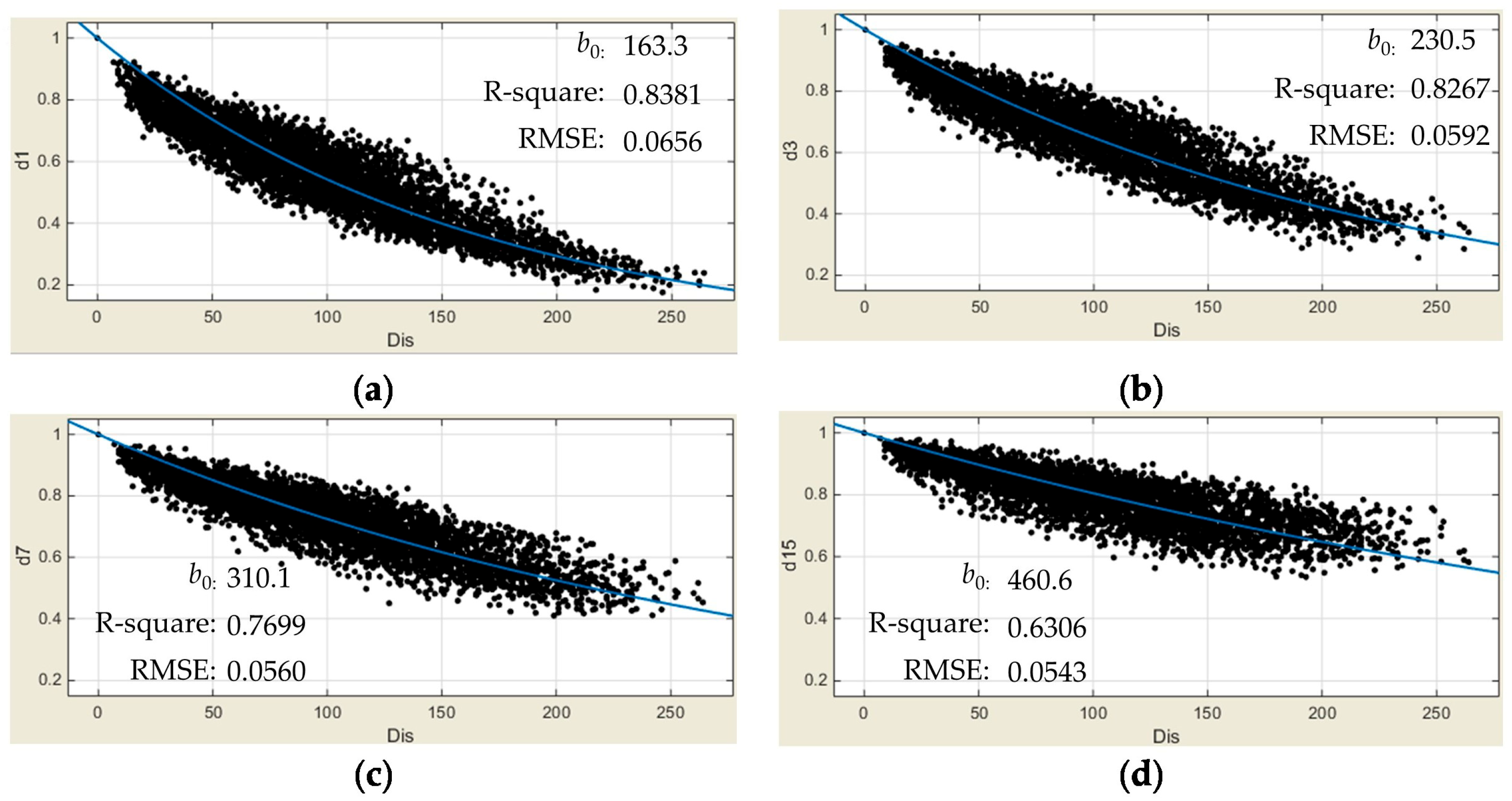
3.1. The Impact of Time Scale and Distance on Rainfall Correlation

The correlation coefficient matrix for all pairs of stations is significant at the p < 0.01 level. The goodness of fit of the model remains virtually unchanged when θ = 1 and when θ is allowed to vary. In alignment with Occam’s Razor, θ = 1 was chosen to simplify the model. Figure 2 displays the inter-station distance–decay correlation coefficient for various time scales, including 1 day, 3 days, 7 days, 15 days (black dots), along with the corresponding fitted curves (blue lines). It was observed that the correlation decreases as the distance between stations increases. The concave shape of the correlograms and their sharp decline at short distances are clearly visible across all time scales, particularly for the daily, 3-day, and 7-day scales. This indicates that the correlation coefficient decays exponentially with distance, a relationship that holds true across the board. It can be seen that the maximum inter-station distance is approximately 265 km. The values for b₀ were 163.3, 230.5, 310.1, 460.6 km for the daily, 3-day, and 7-day scales, respectively. This means that the distance of the correlation coefficient decays to 0.37. Correlations for inter-station distances below 20 km are quite high, ranging from 0.78 to 0.93. Beyond this distance, the correlations gradually decay, but the pattern becomes less clear beyond 230 km, where all correlation coefficients fluctuate around 0.22.

Despite the significant daily rainfall correlation coefficients observed between all pairs of stations, it is evident that these coefficients tend to diminish with increasing spatial distance.

Table 1. Statistical description of the correlation coefficient matrix for different time scales.

Time Scale	1 d	3 d	7 d	15 d
mean	0.555	0.652	0.723	0.799
standard derivation	0.163	0.142	0.117	0.089
coefficient of variation	0.294	0.218	0.162	0.112
minimum	0.176	0.257	0.410	0.534

presents a statistical summary of the correlation for different time scales. It is noticeable that as the time scale increases, the mean and minimum values of the correlation coefficients also increase, while the standard deviation and coefficient of variation decrease. Figure 2 provides the R-square and RMSE (root mean square error) values to assess the goodness of fit of the analytical approximation for different time scales. These metrics offer a comprehensive evaluation of our model using the data at various time intervals. Upon analyzing the relationship between correlation and time scale, Figure 2’s scatter plot illustrates a trend in which the correlation coefficient values increase with the time scale. Specifically, the average correlation coefficient rises from 0.555 to 0.799. The minimum correlation coefficient for the daily time scale is 0.176, while it increases to 0.534 for the 15-day time scale. The coefficient of variation, which is the ratio of the standard deviation to the mean, decreases from 0.294 to 0.058. These changes illustrate that as the time scale increases, the correlation coefficient generally strengthens and exhibits less fluctuation.

From this, two conclusions can be drawn: firstly, the correlation coefficient decays exponentially with distance; secondly, the correlation coefficient increases with larger time scales. An intriguing feature of the fitting results in Table 1 is that the R-square and RMSE values, both indicators of the goodness of fit, tend to move in the same direction. The R-square value indicates how well the model fits the observations, whereas the RMSE value represents the simulation accuracy. This suggests that as the time scale increases, the model’s ability to interpret the dependent variable decreases, while the fitting precision increases. This might seem counterintuitive. However, the simulated data for different time scales exhibit varying distribution characteristics. The R-square value represents the ratio of the sum of squares of the regression (SSR) to the total sum of squares (SST), while the RMSE is the square root of the MSE (mean squared error). Therefore, the RMSE is not a meaningful metric for comparing the goodness of fit across different time scales.

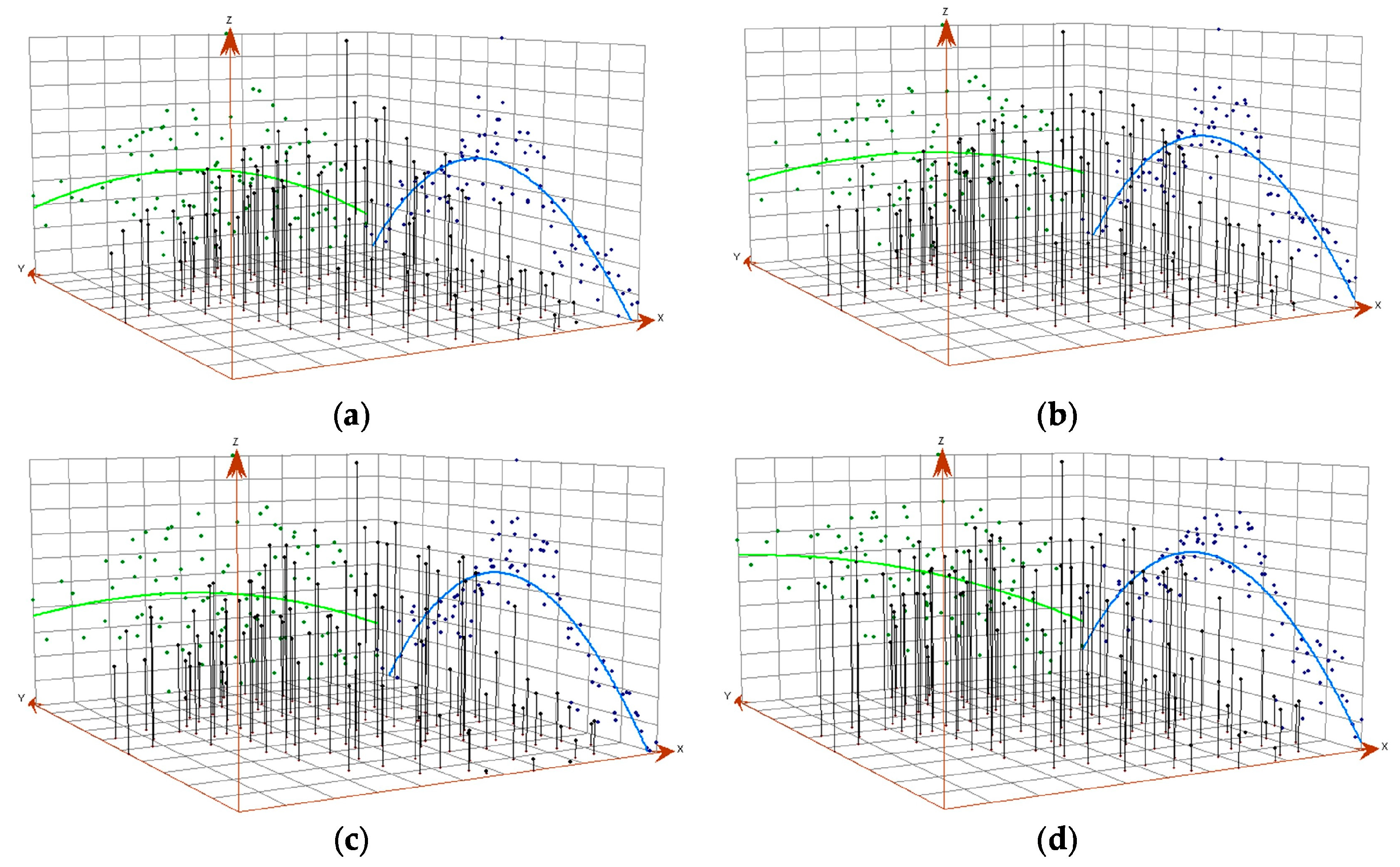
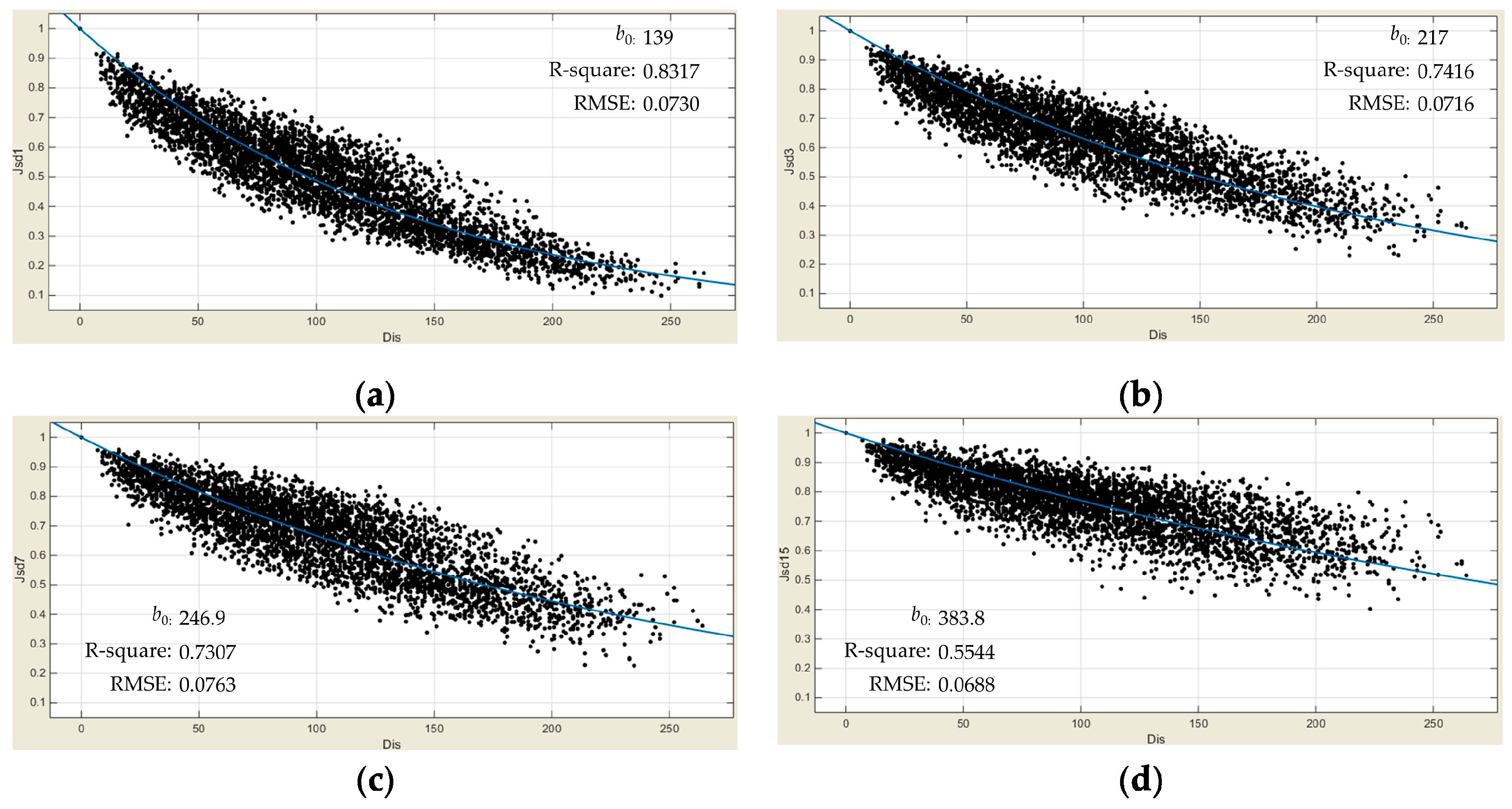
3.2. Spatial Anisotropy of the Correlation Field

To investigate the spatial variability of the correlation field, AnFeng station, located near the center of the study area, was taken as the reference station. This choice enables a comprehensive analysis in all directions. As illustrated in Figure 3, distinct patterns of the correlation coefficient variation are observed along both the x-axis (north–south direction) and y-axis (east–west direction), where the x, y, and z-axes follow the right-hand rule. Along the x-axis, the variation in the correlation coefficient shows no significant trend, as evidenced by the green line. This lack of trend may be attributed to the considerable dispersion of the scatter plot in the XZ plane. In contrast, along the y-axis, a clear trend is evident, with the correlation coefficient decaying as the distance increases in both the northern and southern directions, as shown by the blue line. From these observations, it can be inferred that the correlation field exhibits anisotropy, with a noticeable distance–decay in the longitudinal direction, but there is no significant decay in the latitudinal direction. These findings highlight the importance of accounting for spatial anisotropy when analyzing the correlation structure of rainfall fields.

Researchers have preliminarily identified anisotropic characteristics in the distance–decay of the correlation through their analysis. To further investigate this phenomenon, the correlation field was modeled using the ordinary Kriging method within a geostatistical framework. The Kriging method estimates unknown values as a weighted linear combination of nearby data points, with the objective of minimizing the variance in the prediction error while ensuring that the residuals are close to zero [29]. Although the Kriging approach inherently introduces some degree of error, this does not significantly affect the overall trend observed in the correlation field.

A key advantage of the Kriging method lies in its capacity to effectively represent spatial anisotropy. By leveraging this method, researchers can capture both the spatial variability and directional dependence within the correlation field, thereby providing a more detailed understanding of the anisotropic nature of distance–decay. This methodological approach proves particularly valuable for visualizing and quantifying variations in correlation decay across different spatial directions, ultimately enhancing the ability to model and interpret the spatial structure of rainfall correlations in the study area.

Figure 4 illustrates the distribution of correlation coefficients for the different time scales, which resembles an ellipse with its major axis aligned along the east–west direction and its minor axis along the north–south direction. As the time scale increases, the correlation pattern evolves into a more rectangular shape, possibly due to the constraints of our regional extent. This observation is in agreement with the results from our trend analysis. For the time scale of 15 days, the correlation coefficients are almost consistently above 0.7, which is considered a high correlation in statistical terms. In this flat plain region, the phenomenon indicates that the monsoon climate is the predominant factor influencing the rainfall process. However, it is also evident that the air mass during the monsoon season exhibits a delay in the longitudinal direction. As mentioned earlier, the correlation coefficient for the daily data is above 0.7 within a range of approximately 50 km in the longitudinal direction. This suggests that caution should be exercised when extrapolating to regions without stations at larger spatial scales, as the complexity may increase due to the lack of data points for accurate analysis. Furthermore, the intricacies of the correlation structure may become more pronounced at smaller time scales, such as minutes or hours, where additional factors could influence the rainfall patterns. This highlights the importance of considering the temporal and spatial scales when analyzing rainfall correlations and their driving factors, particularly in the context of a monsoon-influenced climate.

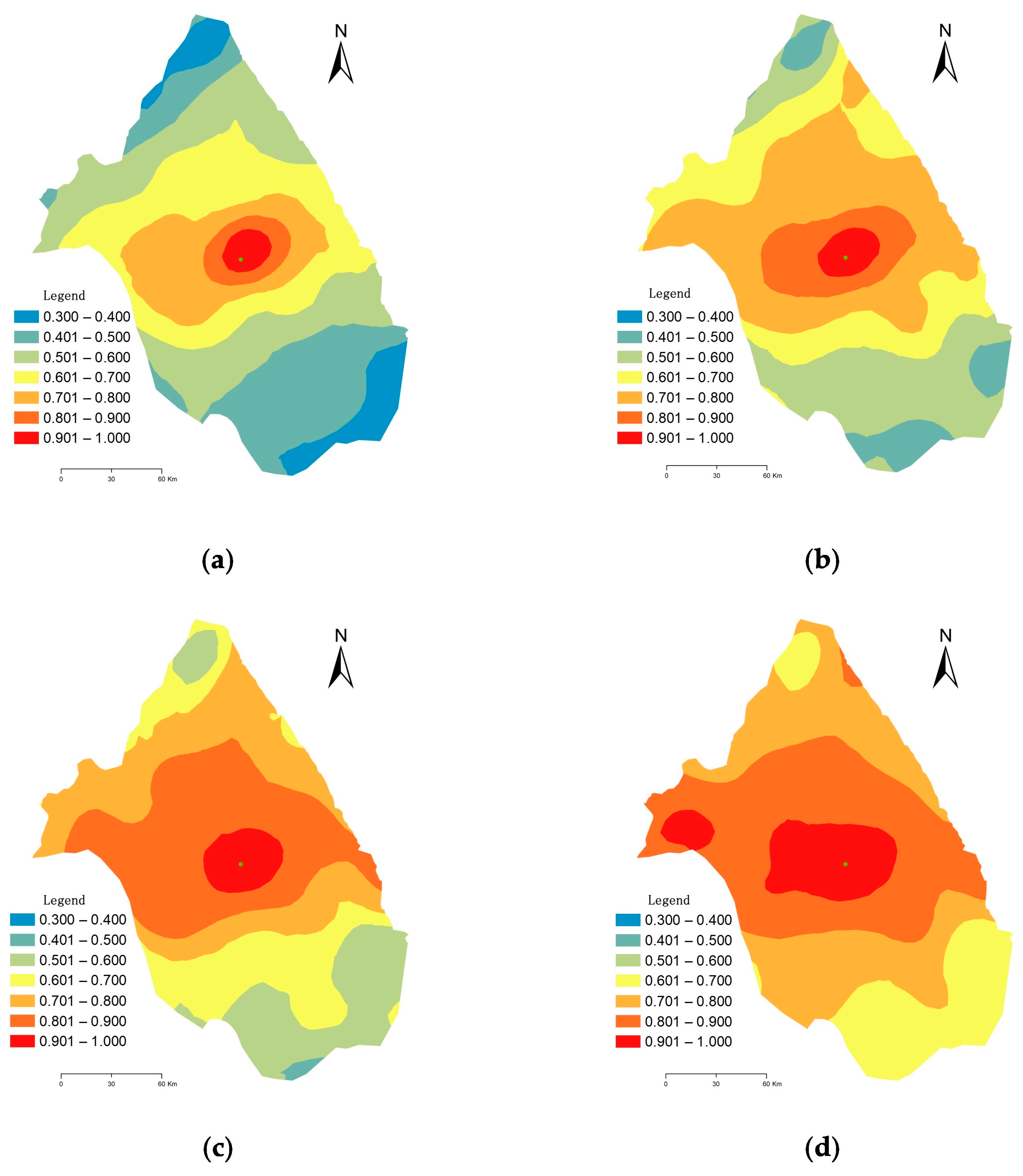
3.3. Character of the Correlation Filed in Wet Season

Since rainfall is predominantly concentrated in the summer and early autumn months, from June to September, accounting for an average of 65.7% of the annual total, the wet season was analyzed separately. Daily rainfall data from June to September over the years 2006 to 2012 were utilized for this analysis. This focused examination facilitates a more detailed understanding of the rainfall patterns during the peak precipitation period, which is essential for various hydrological and meteorological applications.

AnFeng station was also taken as the central point to analyze the spatial correlation field during the wet season. Figure 5 and Figure 6 reveal that the distance–decay and spatial heterogeneity patterns in the wet season are similar to those observed throughout the entire year. However, a closer examination reveals some distinctions between the wet season and the annual patterns. It shows a pattern, as indicated in Figure 2, where the distance–decay coefficients (b₀) in the wet season are smaller than those in the entire year, as indicated in Figure 2. Comparing Figure 6 with Figure 4, it is evident that the area with correlation coefficients above 0.7 during the wet season is smaller than that in the entire year. These observations collectively suggest that the correlation relationships during the wet season are weaker compared to the whole year. The difference in correlation coefficients between the wet season and the entire year is statistically significant, with a paired samples test yielding a difference of 0.048.

4. Discussion

Our findings are largely consistent with those of other studies [25,30], which also observed a concave shape in the correlograms. However, there are differences with studies by Grzegorz [24], where the correlograms showed a convex shape. This discrepancy may be attributed to the fact that the time resolution was 0.5 s and the spatial scale was approximately 3 km by 3 km, whereas in our study, the time resolution is at the daily level, with the maximum inter-station distance reaching about 264 km. These differences in scale likely contribute to the variations in the shape of the correlograms observed across studies.

The presence of completely dry days throughout the year likely contributes to this result, as these days can elevate the correlation coefficient, as demonstrated in various studies in the literature [14,19,23,24]. The correlation coefficient for the wet season, based on data with completely dry days removed, showed a significant difference from the raw data. A paired samples test yielded a difference of 0.018. However, this difference is smaller than the difference in correlation coefficients between the wet season and the entire year. This leads us to conclude that the variability in rainfall during the wet season also contributes to the lower correlation coefficients. The mean daily rainfall for all stations from June to September is 5.50 mm with a standard deviation of 15.36 mm, whereas the mean daily rainfall for the entire year is 2.80 mm with a standard deviation of 9.93 mm. This indicates that rainfall variability in the wet season is higher, which aligns with findings from a study in the southeast USA [29].

5. Conclusions

The distance–decay of rainfall correlation is significant across different time scales, and an exponential function adequately captures this decay, assuming spatial isotropy. However, it is important to note that this characteristic varies markedly for different time scales. The rate of the distance–decay correlation coefficient decreases as the time scales increase. For example, the parameter b₀ is 163.3 km at the daily scale, which is significantly smaller than the 460.6 km at the 15-day scale. The area with correlation coefficients above 0.7 expands as the time scale increases. For daily data, this area is only about 50 km in latitude and 150 km in longitude, whereas for the 15-day data, all areas exceed 0.7.

Given that the study area is a low-lying plain with elevations ranging from −4 to 17 m, the influence of the topography on the correlation field changes is minimal. Additionally, the coastal region does not exhibit a significant difference in the correlation field. In flat plain regions primarily affected by large-scale atmospheric air masses, it is reasonable to interpolate daily rainfall at distances within 50 km and up to 15 days within 150 km. However, when the distances exceed 163.3 km, the correlation drops to around 0.37, which is relatively weak, thus warranting caution in interpolation.

An intriguing observation is that the area with correlation coefficients above 0.7 during the wet season is about 100 km² smaller than the corresponding area for the entire year. This discrepancy may be attributed to the impact of completely dry days, as suggested by previous research. When the correlation coefficients were calculated excluding data from completely dry days, the change was only a decrease of 0.018. On the other hand, rainfall variability during the wet season led to a reduction in the correlation coefficient by 0.048. This implies that rainfall variability in the wet season is higher than that observed throughout the entire year.

References

1. Hwang, Y.; Clark, M.; Rajagopalan, B.; Leavesley, G. Spatial interpolation schemes of daily precipitation for hydrologic modeling. Stoch. Environ. Res. Risk Assess. 2012, 26, 295–320. [Google Scholar] [CrossRef]
2. Xu, W.; Zou, Y.; Zhang, G.; Linderman, M. A comparison among spatial interpolation techniques for daily rainfall data in Sichuan province, China. Int. J. Climatol. 2015, 35, 2898–2907. [Google Scholar] [CrossRef]
3. Elumalai, V.; Brindha, K.; Sithole, B.; Lakshmanan, E. Spatial interpolation methods and geostatistics for mapping groundwater contamination in a coastal area. Environ. Sci. Pollut. Res. 2017, 24, 11601–11617. [Google Scholar] [CrossRef]
4. Yeh, H.C.; Chen, Y.C.; Wei, C.; Chen, R.H. Entropy and kriging approach to rainfall network design. Paddy Water Env. 2011, 9, 343–355. [Google Scholar] [CrossRef]
5. Wang, Y.; Liu, X.; Liu, R.; Zhang, Z. Research Progress on Spatiotemporal Interpolation Methods for Meteorological Elements. Water 2024, 16, 818. [Google Scholar] [CrossRef]
6. Fassnacht, S.R.; Dressler, K.S.; Bales, R.C. Snow water equivalent interpolation for the Colorado River Basin from snow telemetry (SNOTEL) data. Water Resour. Res. 2003, 39, 1208. [Google Scholar] [CrossRef]
7. Garcia, M.; Peters-Lidard, C.D.; Goodrich, D.C. Spatial interpolation of precipitation in a dense gauge network for monsoon storm events in the southwestern United States. Water Resour. Res. 2008, 44, 387–400. [Google Scholar] [CrossRef]
8. Li, X.; Heap, A.D. A review of comparative studies of spatial interpolation methods in environmental sciences. Environ. Model. Softw. 2014, 51, 1–12. [Google Scholar]
9. Song, L.; Tian, Y.; Wu, L.; Zhang, H. On Comparison of Spatial Interpolation Methods of Daily Rainfall Data: A Case Study of Shenzhen. J. Geo-Inf. Sci. 2008, 10, 566–572. [Google Scholar]
10. Chen, D.; Ou, T.; Gong, L.; Xu, C.-Y.; Li, W.; Ho, C.-H.; Qian, W. Spatial interpolation of daily precipitation in China: 1951–2005. Adv. Atmos. Sci. 2010, 27, 1221–1232. [Google Scholar] [CrossRef]
11. Karakaya, N.; Demirtaş, N. A comparison of interpolation techniques for predicting groundwater levels in urban areas. Hydrol. Res. 2022, 53, 94–106. [Google Scholar]
12. Das, M.; Hazra, A.; Sarkar, A.; Bhattacharya, S.; Banik, P. Comparison of spatial interpolation methods for estimation of weekly rainfall in West Bengal, India. Mausam 2017, 68, 41–50. [Google Scholar] [CrossRef]
13. Hendrick, R.L.; Comer, G.H. Space variations of precipitation and implications for raingage network design. J. Hydrol. 1970, 10, 151–163. [Google Scholar] [CrossRef]
14. Stol, P.T. The relative efficiency of the density of rain-gage networks. J. Hydrol. 1972, 15, 193–208. [Google Scholar] [CrossRef]
15. Jackson, I.J. Inter-station rainfall correlation under tropical conditions. CATENA 1973, 1, 235–256. [Google Scholar] [CrossRef]
16. Jackson, I.J. Local differences in the patterns of variability of tropical rainfall: Some characteristics and implications. J. Hydrol. 1978, 38, 273–287. [Google Scholar] [CrossRef]
17. Sharon, D. Correlation Analysis of the Jordan Valey Rainfall Field. Mon. Weather Rev. 2009, 107, 1042–1047. [Google Scholar] [CrossRef]
18. Baldassare, B.; Kottegoda, N.T. Identification and calibration of spatial correlation patterns of rainfall. J. Hydrol. 1995, 165, 311–348. [Google Scholar]
19. Sumner, G.N. The use of correlation linkages in the assessment of daily rainfall patterns. J. Hydrol. 1983, 66, 169–181. [Google Scholar] [CrossRef]
20. Trinugroho, M.W.; Arif, S.S.; Susanto, S.; Nugroho, B.D.A.; Prabowo, A. Changes in Rainfall Pattern in Bengawan Solo Sub-Watershed. Sains Tanah J. Soil Sci. Agroclimatol. 2022, 19, 249–260. [Google Scholar] [CrossRef]
21. Ding, Y.; Chan, J. The East Asian summer monsoon: An overview. Meteorol. Atmos. Phys. 2005, 89, 117–142. [Google Scholar]
22. Chen, J.; Lu, D. Division of monsoon climatic regions in China. J. Beijing For. Univ. 1981, 4, 1–8. [Google Scholar]
23. Berndtsson, R. On the use of cross-correlation analysis in studies of patterns of rainfall variability. J. Hydrol. 1987, 93, 113–134. [Google Scholar] [CrossRef]
24. Bonell, M.; Sumner, G. Autumn and winter daily precipitation areas in Wales, 1982–1983 to 1986–1987. Int. J. Climatol. 1992, 12, 77–102. [Google Scholar] [CrossRef]
25. Habib, E.; Krajewski, W.F.; Ciach, G.J. Estimation of rainfall interstation correlation. J. Hydrometeorol. 2001, 2, 621–629. [Google Scholar] [CrossRef]
26. Ciach, G.J.; Krajewski, W.F. Analysis and modeling of spatial correlation structure in small-scale rainfall in Central Oklahoma. Adv. Water Resour. 2006, 29, 1450–1463. [Google Scholar] [CrossRef]
27. Bekas, G.K.; Alexakis, D.E.; Gamvroula, D.E. Forecasting discharge rate and chloride content of karstic spring water by applying the Levenberg-Marquardt algorithm. Environ. Earth Sci. 2021, 80, 404. [Google Scholar] [CrossRef]
28. Lourakis, M.I.A. A brief description of the Levenberg-Marquardt algorithm implemented by levmar. Found. Res. Technol. 2005, 4, 1–6. [Google Scholar]
29. Baigorria, G.A.; Jones, J.W.; O‘Brien, J.J. Understanding rainfall spatial variability in southeast USA at different timescales. Int. J. Climatol. 2010, 27, 749–760. [Google Scholar] [CrossRef]
30. Dzotsi, K.A.; Matyas, C.J.; Jones, J.W.; Baigorria, G.; Hoogenboom, G. Understanding high resolution space-time variability of rainfall in southwest Georgia, United States. Int. J. Climatol. A J. R. Meteorol. Soc. 2014, 34, 3188–3203. [Google Scholar] [CrossRef]
Figure 1. Layout of rainfall stations (AnFeng station marked in red). The values near the stations on the right figure represent the manually assigned codes for the rainfall stations.
Water 17 00654 g001
Figure 2. The correlation coefficient decay with distance at different time scales of (a) daily, (b) 3 days, (c) 7 days, and (d) 15 days. The vertical axis represents the correlation coefficient (a dimensionless quantity), and the horizontal axis represents the distance in kilometers (km). The blue line represents the curve fitted using Formula (2).
Water 17 00654 g002
Figure 3. The correlation coefficient (z-axis) trend for time scales of (a) daily, (b) 3 days, (c) 7 days, and (d) 15 days. The x-axis represents the north–south direction, the y-axis represents the east–west direction, and the z-axis shows the correlation coefficient. The blue curve represents the fitted trend projected onto the y-axis, with blue points indicating the projections on the y-axis, while the green curve represents the fitted trend projected onto the x-axis, with green points indicating the projections on the x-axis.
Water 17 00654 g003
Figure 4. Correlation field generated by the Kriging method for time scales of (a) daily, (b) 3 days, (c) 7 days, and (d) 15 days. AnFeng station is marked with a green dot.
Water 17 00654 g004
Figure 5. The correlation coefficient decay in the wet season with distance for time scales of (a) daily, (b) 3 days, (c) 7 days, and (d) 15 days. The vertical axis represents the correlation coefficient (a dimensionless quantity), and the horizontal axis represents the distance in kilometers (km). The blue line represents the curve fitted using Formula (2).
Water 17 00654 g005
Figure 6. Correlation field generated by the Kriging method in the wet season for time scales of (a) daily, (b) 3 days, (c) 7 days, and (d) 15 days. AnFeng station is marked with a green dot.
Water 17 00654 g006