1. Introduction
The coast is the boundary between the ocean and the land, characterized by the significant impact of waves and tides, where the interaction and contact between the ocean and land occur. Over the years, coastal landslide disasters have received widespread attention due to the needs of coastal beach tourism, coastal ecological environment protection, and coastal economic zone development [
1,
2]. However, more attention has been paid to gravelly coasts, muddy coasts, wetland coasts, and artificial coasts, while the long-term geological disaster risks of rocky coastal zones have been overlooked. In fact, rocky coastal zones have experienced numerous landslide disasters under long-term internal and external dynamic geological conditions, such as wave, tidal, and seismic dynamic loads, adversely affecting the safety of construction projects in these coastal zones [
3,
4,
5,
6].
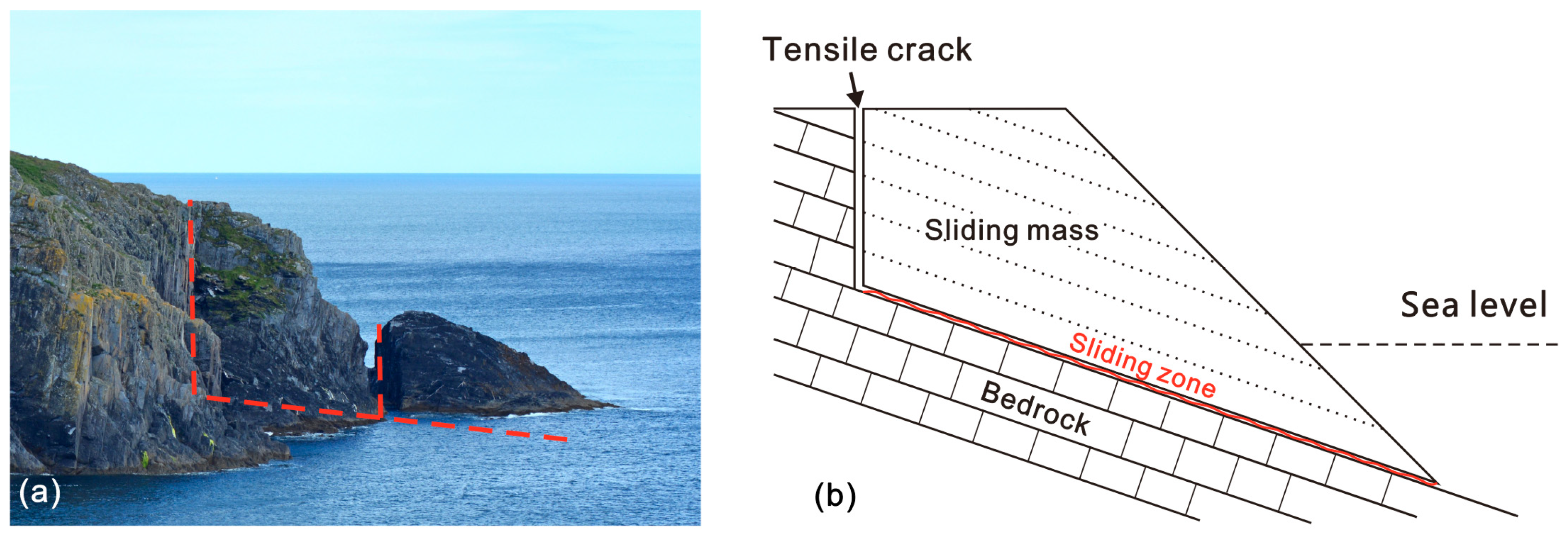
The rocky coastlines present in nature are predominantly characterized by steep slopes. However, some coastlines are influenced by the dip angles of rock layers and specific structural planes, which may lead to the formation of relatively gentle slopes over certain time periods. This research focuses on localized rocky slopes within the wave impact zone.
Figure 1 shows a typical photo of a coastal rocky slope and a generalized geological model. The stability and deformation failure modes of coastal rocky slopes are primarily controlled by weak structural planes within the rock mass, which possess relatively lower strength. The structural plane with a gentle dip angle at the bottom of the sliding mass, often comprising bedding planes or joint planes, forms the potential sliding surface. Conversely, the steeply dipping or vertical structural planes located at the rear of the sliding mass, typically consisting of joint planes and faults, constitute the rear boundary of the sliding mass [
7,
8].
There are various methods for calculating and analyzing the stability of terrestrial rocky slopes, which can be broadly categorized into theoretical analysis methods and numerical analysis methods [
9]. Theoretical analysis methods include graphical methods (e.g., stereographic projection) and the limit equilibrium method, while numerical analysis methods encompass the finite element method, discrete element method, boundary element method, and numerical manifold method [
10,
11,
12]. Among these, advanced numerical analysis methods can accurately describe the mechanical behavior and failure process of complex landslide bodies, but the accuracy of their results depends on reliable geological models and computational parameters. On the other hand, the LEM, despite being based on simplified assumptions, offers a straightforward and intuitive calculation process that is easy to implement. Its results are deterministic and reproducible, making it a classic method widely used in engineering practice for landslide stability analysis [
13].
The limit equilibrium method is currently the most widely used method for analyzing the stability of terrestrial rocky slopes. The basic principle of this method is to consider the landslide body as a system in a critical equilibrium state. By calculating the mechanical equilibrium conditions on the potential sliding surface, the stability of the landslide can be evaluated [
14]. However, unlike terrestrial rocky slopes, coastal rocky slopes are subject to additional loads beyond gravity, hydrostatic pressure, and seismic forces, specifically the long-term effects of wave loading. Under long-term cyclic loading, geomaterials may experience fatigue failure, especially within coastal rock mass where weak structural planes may form potential sliding surfaces [
15,
16]. Structural planes in natural rock masses often contain filling materials such as clay, sand, and highly weathered rock fragments. Under prolonged cyclic wave loading, the slope body above the structural plane experiences slight oscillations, leading to minor displacements along the weak plane. The strain-softening phenomenon caused by fatigue damage to the filling materials alters the mechanical properties of the structural plane and the overall strength of the rock mass, thereby reducing the stability of the rocky slope body. Over time, this cumulative effect can trigger landslide disasters [
17,
18].
To study the impact of long-term wave loading on the stability of coastal rocky slopes, we first utilized fluid dynamics programs to analyze the magnitude and distribution characteristics of wave pressure on slopes with varying angles under different wave heights. These pressure were then decomposed to determine the shear stress components along the potential sliding surfaces of the landslides. Based on the constitutive model of strain-softening in geomaterials, we analyzed the long-term weakening pattern of shear strength caused by the variation in shear stress due to wave action on the sliding surface. Consequently, we proposed a method for calculating the long-term factor of safety (FOS) of coastal rocky slopes under the influence of wave loading.
2. Mechanical Model of Coastal Rocky Slope
By comprehensively analyzing the geological structural characteristics and macroscopic failure modes of coastal rocky slopes, it is evident that the failure mechanism of coastal rocky slopes primarily involves sliding along weak planes such as bedding planes, joint planes, and fracture planes under unfavorable combinations of structural planes. The failure mode of coastal rocky slopes can be simplified into the generalized geological model shown in
Figure 1b. In this model, a set of gently inclined weak planes dipping towards the slope face generally forms the potential sliding surface of the landslide, while steeply inclined structural planes with orientations consistent with the slope surface at the rear of the rocky coast typically constitute the rear boundary of the rocky slope. If the rocky coast contains these two sets of intersecting unfavorable structural planes, there exists a significant risk of sliding failure.
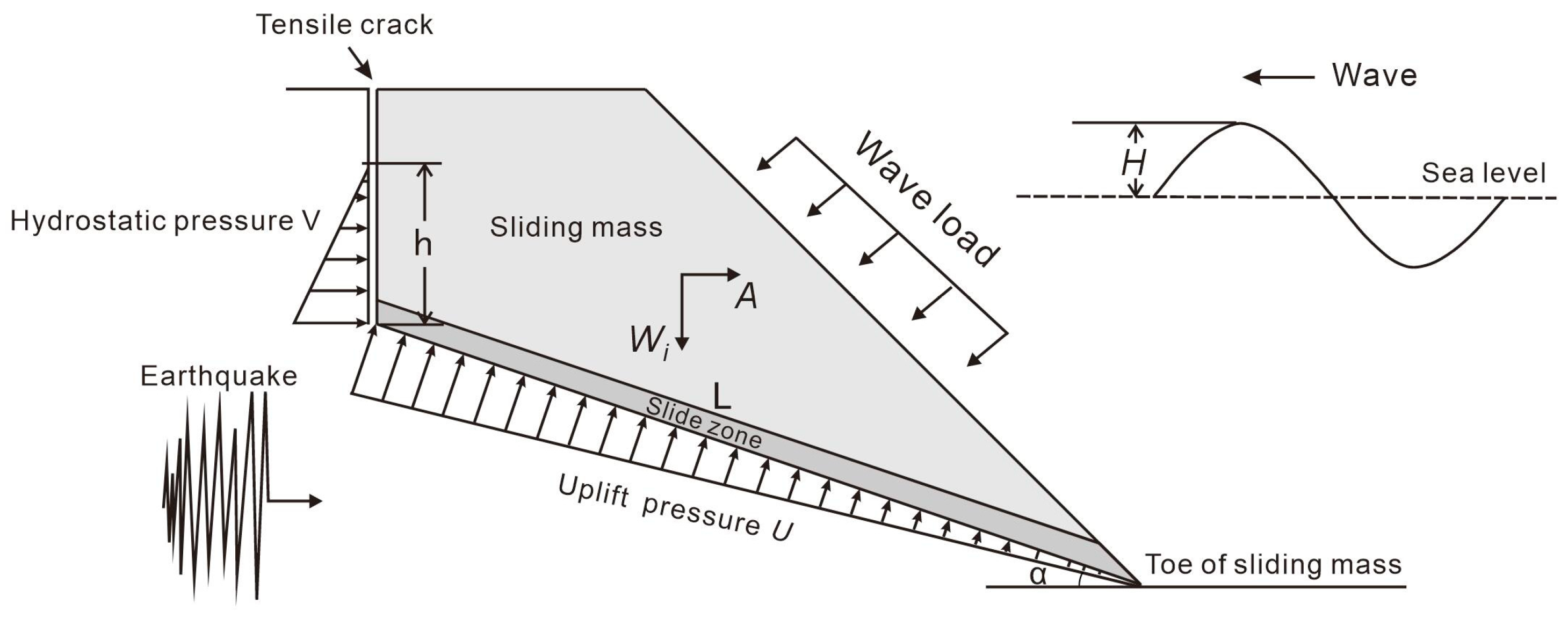
Based on the mechanical calculation model for the stability of terrestrial rockslides [
13], and considering the influence of wave loads, the mechanical model of coastal rocky slopes, as illustrated in
Figure 2, can be obtained. The loads acting on the landslide body are categorized into basic loads and special loads. Basic loads include self-weight, hydrostatic pressure on the rear tensile crack, and uplift pressure on the sliding surface related to underground water and wave load, which occur frequently. Special loads encompass seismic loads and other less frequent loads. Due to prior erosion by seawater, historical pressures, and earthquake disturbances, the interlayer material is in a strain-weakening stage. Additionally, the disturbance from waves, though minor, cumulatively reduces the shear strength of the weakening interlayer over a long period. When the shear strength decreases to the point where it can no longer resist the shear stress caused by the weight of the upper sliding mass, a landslide disaster may occur.
The current stability of coastal rocky slopes, without considering the influence of dynamic wave loads, is assessed using the same limit equilibrium method utilized for terrestrial rocky slope stability calculations. In analyzing the current stability of coastal rocky slope, the main considerations are the resisting forces and driving forces on the potential sliding weak plane. The driving forces mainly include the component of the sliding mass weight along the weak plane, the hydrostatic pressure component along the sliding plane from fractures at the rear of the sliding mass. The resisting force of the weak plane in rocky slopes primarily depends on the normal stress on the weak plane, which includes the component of the sliding mass weight perpendicular to the weak plane, uplift pressure along the weak plane, and the cohesion of the weak plane.
Referring to the computational model in
Figure 2, the current FOS (Kc) of coastal rocky slopes is calculated based on the rigid body limit equilibrium method as the ratio of total resisting force to total driving force [
13]. The specific calculation formula is as follows:
where Kc is the current FOS; W is the weight of the sliding mass; V is the water pressure in rear fractures:
; U is the uplift pressure along the sliding surface:
; h is the water depth in rear fractures; A is the seismic acceleration;
is the friction angle of the sliding surface;
is the cohesion of the sliding surface;
is the slope angle;
is the dip angle of the sliding surface.
Compared with terrestrial rocky slopes, the basic loads considered in the stability calculation of coastal rocky slopes include gravity, water pressure, wave forces, and seismic forces. Due to the relatively high stiffness of rocky slope materials, the sliding mass can be simplified as a rigid body with no deformation. Its gravitational force can be simplified as a constant body force acting vertically downward at the center of mass. Water pressure includes hydrostatic pressure acting on the rear boundary of the landslide and uplift pressure on the bottom sliding surface, calculated based on the seawater level corresponding to the design tide level, numerically equal to the pressure head at the point of application. Since rocky slopes generally do not involve soil liquefaction mechanisms, seismic loads are considered only in terms of inertial forces, calculated using the pseudo-static method [
19]. The wave force mechanisms acting on coastal rocky slopes are complex, involving full reflection, partial reflection, and breaking waves. The energy attenuation and transformation are influenced by these reflection and breaking conditions [
20].
3. Calculation Method of Wave Pressure on Coastal Rocky Slope
Flow-3D computational fluid dynamics software is widely used for numerical simulations of wave analysis and has been validated by numerous studies to accurately simulate wave motion characteristics and their interactions with solid bodies [
21,
22]. Considering that waves are characterized by incompressible viscous fluid motion, Flow-3D employs the continuity equation for liquid motion and the Navier–Stokes equations for incompressible viscous fluid motion as the governing equations. Its unique FAVOR grid processing technology allows the definition of independent complex geometries within structured grids, achieving the representation of arbitrarily complex geometrical shapes using simple rectangular grids [
23].
Flow-3D (V11.2) provides various turbulence models. Among them, the RNG k-ε model, which modifies turbulent viscosity and considers rotational and swirling flows in the mean flow, is better suited for handling flows with significant streamline curvature and high strain rates [
24]. Flow-3D uses the volume of fluid method to calculate the fluid volume fraction within grid cells, tracking the interface between two immiscible fluids [
25]. This method effectively tracks the free surface of complex deformations, where the two immiscible fluids are water and air. Since wave motion is a transient problem, the computational domain needs to be discretized in both space and time before solving the governing equations of motion. For this purpose, Flow-3D employs the finite difference method for discretization, with the spatial domain divided into three-dimensional rectangular staggered grids. Scalars such as pressure, density, and fluid volume fraction are defined at the center of the control volume, while vectors such as velocity are defined at the center of the grid boundary faces [
26].
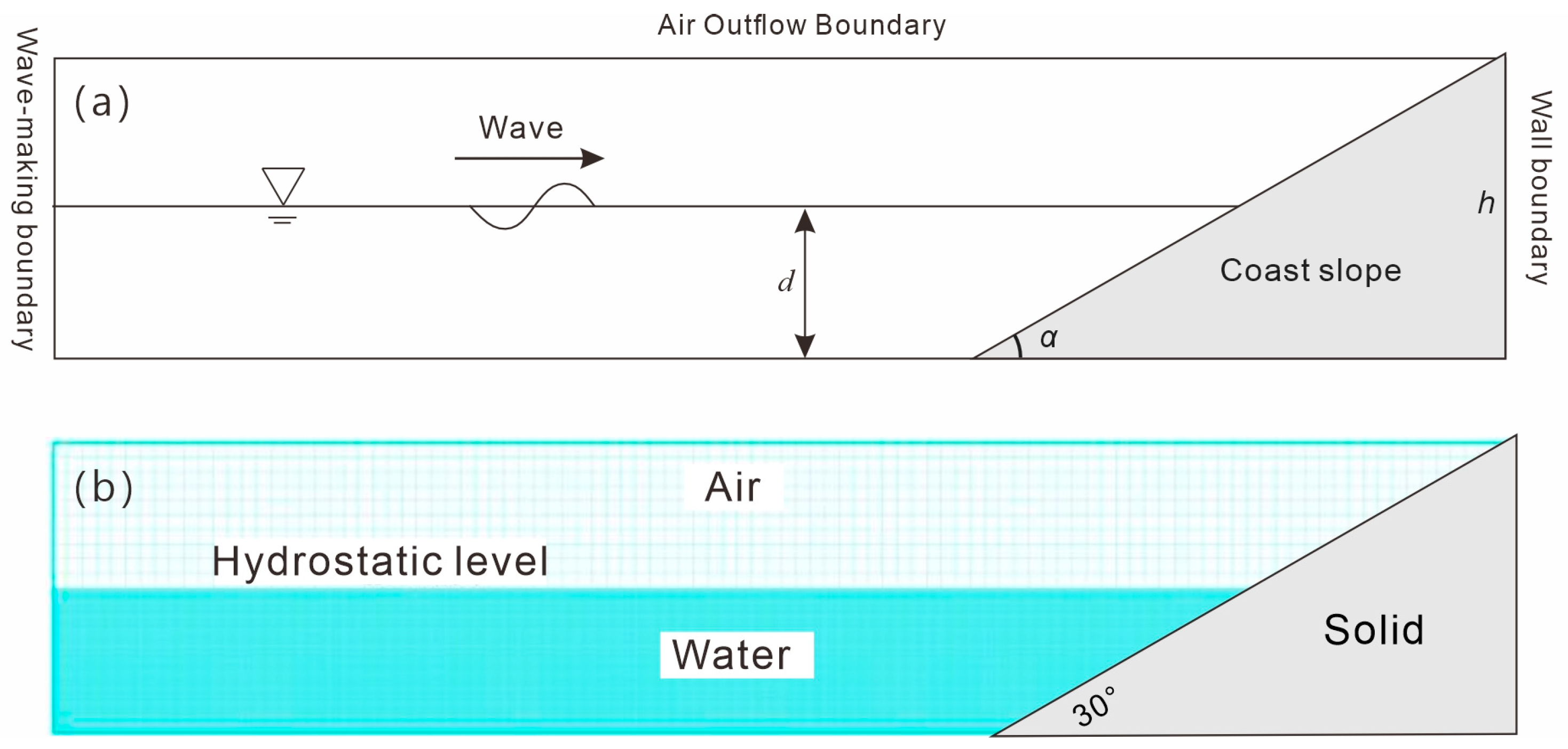
The two-dimensional computational model was drawn using ZWCAD2024 software, as shown in
Figure 3a. In this model, the triangular solid region on the right represents a coastal rocky slope with a certain incline, while the water area on the left simulates the nearshore ocean in front of the slope. To study the impact characteristics of waves with different heights on coastal rocky slopes with various inclines, the coastal slope in this model was set with inclines of 30°, 45°, 60°, 75°, and 90°. The model consists of a 200 m horizontal wave surge area and the base of the slope, with the z-direction representing a slope height of 30 m. The still water depth, d, in front of the slope was set to half the slope height, i.e., 15 m.
The aforementioned computational model was assigned materials and meshed as shown in
Figure 3b. In this setup, the rocky slope is designated as a non-moving solid material. The region below the hydrostatic level in the water area is set as water, while the region above is set as air. The fluid region of the model was meshed with grid sizes of 0.5 m in both the horizontal and vertical directions. When setting the boundary conditions for the model, the right and bottom sides of the model were defined as wall boundary conditions. The top side was set as an air free outflow boundary, and the left side of the model was set as an active absorption-type elliptic cosine wave generation boundary.
The gravitational acceleration and the viscosity coefficient of the sea water were set to −9.81 m/s2 and 0.007 P, respectively. The simulation duration was set to 120 s. If the simulation time is set too short, the wave load on the coastal slope will not reach a stable pattern, thus affecting the accuracy of the experiment. Conversely, if the simulation time is set too long, it may result in unnecessary computations during the simulation process, reducing simulation efficiency. The initial time step was set to 0.001 s, and the minimum time step was set to 1 × 10⁻⁷ s to ensure the convergence of the simulation. The output settings directly influence the thoroughness and accuracy of the simulation results, and an appropriate output frequency is beneficial for identifying the maximum pressure on the slope under wave loading.
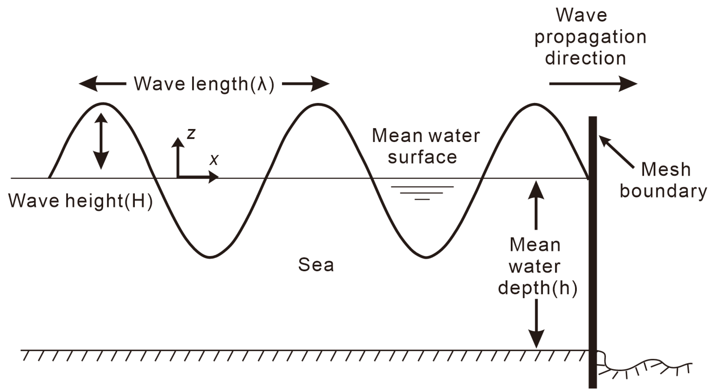
Flow-3D employs the boundary wave generation method, which sets values at the wave generation boundary based on the analytical solution of progressive waves. It assumes that the waves propagate from a flat seabed outside the computational domain into the domain, solving the fluid motion N-S equations within the computational domain to achieve wave generation [
27]. Using the linear sinusoidal wave generation method, three different wave heights (H) of 2 m, 4 m, and 6 m were set for slope models with varying slope angles. The wavelength was uniformly set to 40 m. As shown in the figure below (
Figure 4), a linear wave has a sinusoidal profile with an amplitude that is small relative to the wave length and water depth.
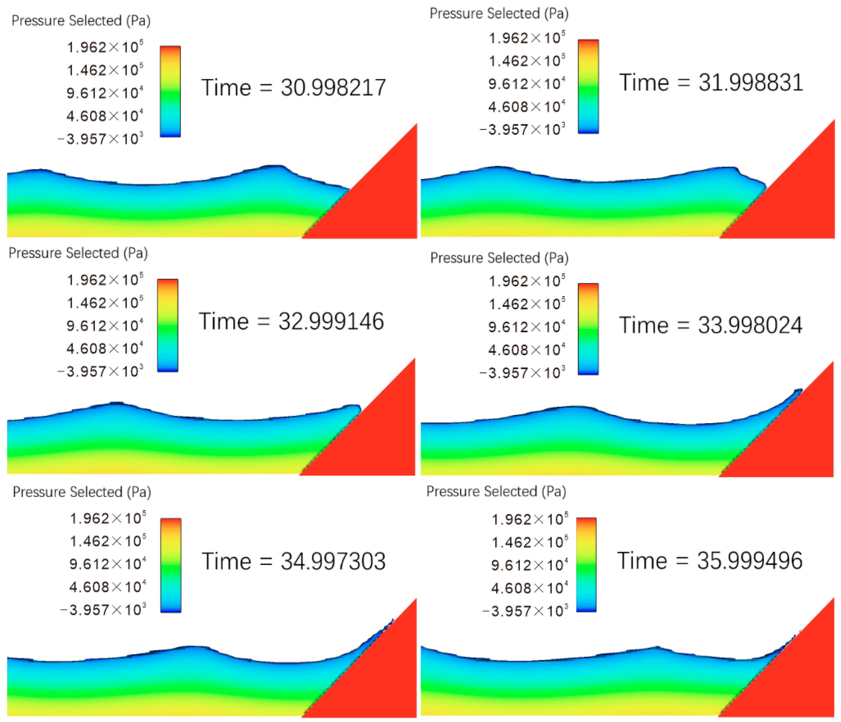
Since the maximum wave pressure impact on the slope surface will directly affect the shear stress and stability of weak structural planes, the focus will now be on analyzing the pattern of the maximum wave pressure.
Figure 5 shows the process of forming the maximum wave pressure on the slope surface with a slope angle of 30° and a wave height H = 4 m. At this point, the wave steepness exceeds the limit load condition when the previous wave has completely receded (no water cushion layer on the slope surface), causing the wave to break and impact the slope surface. This impact generates a maximum wave impact force at the point of impact, referred to as the maximum wave pressure.
4. Wave Load Calculation Results
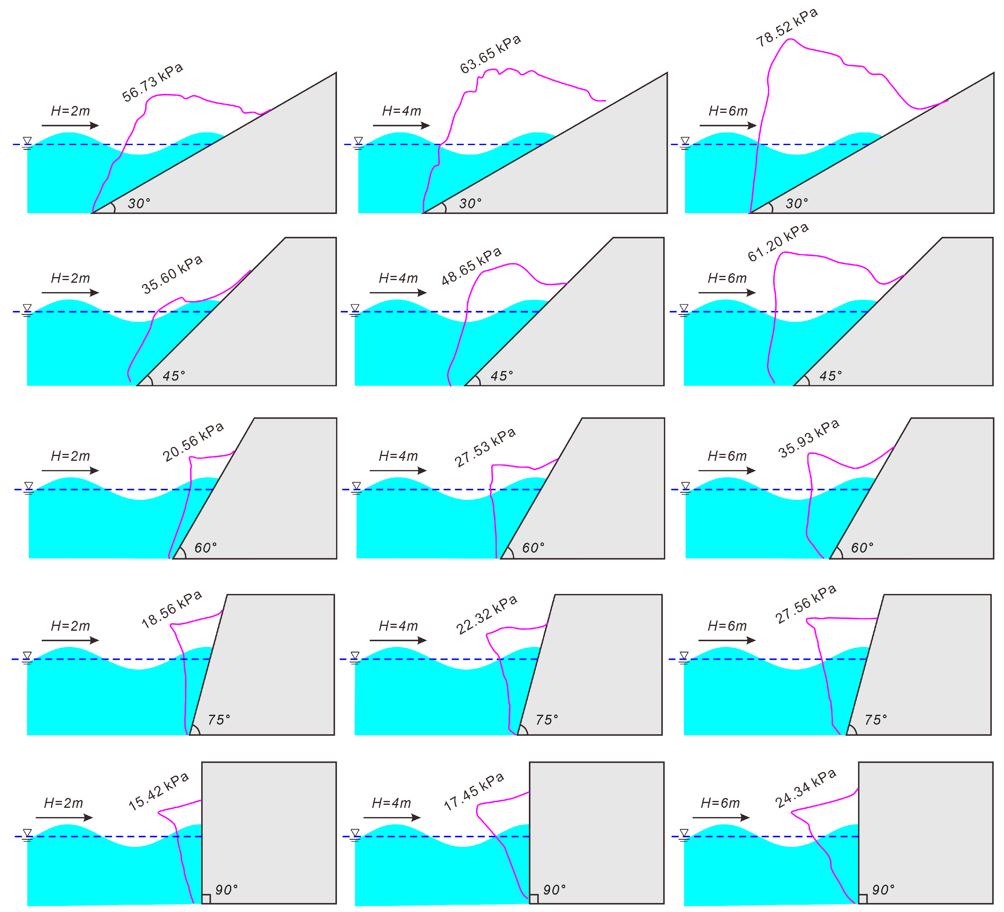
After conducting 15 simulation calculations for each of the five slope angle models under three different wave height conditions, the distributions of wave pressure on the slope surfaces were obtained.
Figure 6 shows the wave pressure distribution curves and maximum pressure values at the moment of maximum wave pressure impact for different scenarios.
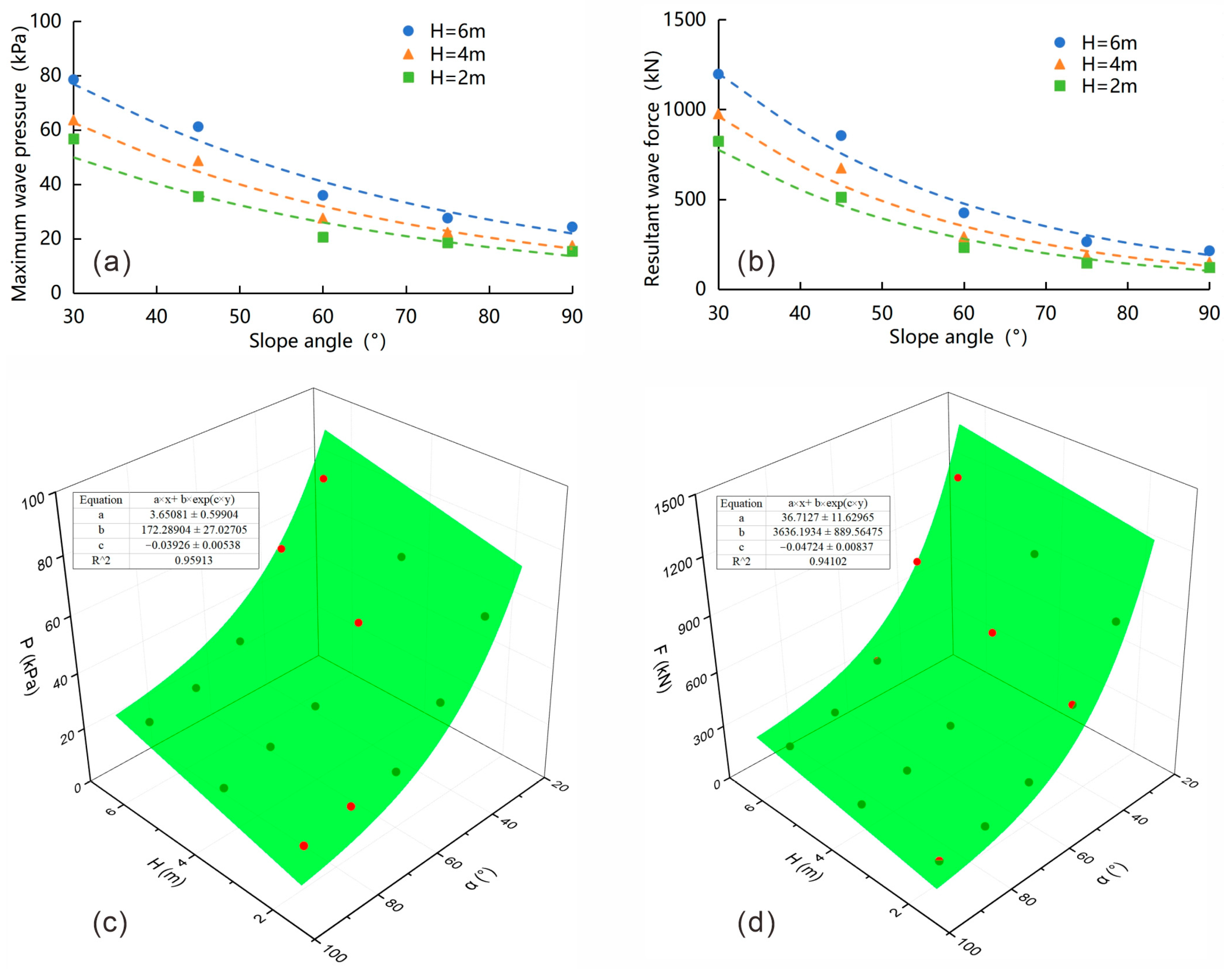
The comparative relationship of the maximum pressure values on the slope surface under different slope angles and wave heights is shown in
Figure 7a. It can be observed that the maximum wave pressure on the slope surface decreases with increasing slope angle and decreasing wave height. By integrating the wave pressure curves of each simulation condition over the slope surface area, the resultant wave forces acting on slopes can be calculated (
Figure 7b). These resultant forces also exhibit a decreasing trend with increasing slope angles and decreasing wave heights. The relation of maximum wave pressure and forces with wave heights and slope angles shows an exponential relationship, which can be fitted by the following model. The nonlinear fitting surface presented in
Figure 7c,d demonstrates that the mathematical model represented by Equation (2) effectively captures the relationship between the maximum wave pressure, resultant wave force, wave height, and slope angle, achieving a R
2 value of approximately 0.95.
where F is the resultant wave pressure; H is the wave height;
is the slope angle; a, b, c are the model fitting parameters.
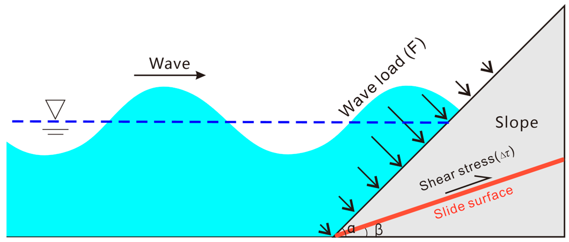
When wave loading acts on the slope surface, the direction of the force is perpendicular to the slope surface. Given that the potential sliding plane of coastal rocky slopes has a gentler dip angle than the slope surface, the change in shear stress on the potential sliding plane caused by wave loading can be derived through conversion. The calculation method is illustrated in
Figure 8. The forces exerted by waves on the slope surface arise from two main components: the weight of the water and the kinetic energy of the water. Through numerical simulations, we have determined that for slopes with relatively gentle inclinations, wave pressure is larger than that on steeper slopes. This is primarily due to the increased gravitational force acting on the relatively gentle slope, as more water accumulates on the slope surface as waves propagate toward the shore. However, as illustrated in the schematic diagram of
Figure 8, although the total wave pressure on the surface of the relatively gentle slope is larger, the shear component acting on the potential sliding surface may not be significant. This depends on the angle between the potential sliding surface and the slope surface.
The change in shear stress on the sliding plane varies with the slope surface inclination and the sliding plane dip angle. The wave load perpendicular to the slope surface can be decomposed along the weak plane, with the component along the weak plane calculated using the following Equation (3).
where
is the shear force due to wave pressure on the sliding surface; F is the resultant wave pressure, which can be calculated by Equation (1) with specific wave height and slope angle;
is the slope angle;
is the weak plane dip angle.
5. Discussion
In the stability analysis of coastal rocky slopes, both current stability and long-term stability must be considered. Current stability refers to the stability of the potential sliding surface of the rocky slope under the present mechanical parameters and boundary conditions. Long-term stability refers to the changes in stability of the potential sliding surface during the strain-softening process under prolonged wave loading.
To calculate the slope stability, it is first necessary to sample the weak plane material and conduct laboratory shear tests to obtain basic physical parameters, such as the friction angle, cohesion, strain-softening displacement, and strain-softening coefficient of the weak plane material. Based on different working conditions, the change in shear force on the weak plane due to wave impact is then calculated. During the stability of the potential sliding weak plane calculating, first, using the measured parameters and data, the shear strength and shear stress of the weak plane are calculated, and the current FOS of the weak plane is determined.
For the long-term stability calculation, it must first be determined whether the shear stress on the weak plane has reached the fatigue failure threshold of the weak plane material. If the shear stress induced by wave pressure does not reach the fatigue failure threshold of the material, the rocky slope will not experience fatigue failure due to wave action, and a long-term stability calculation is unnecessary. However, if the peak shear stress exceeds the fatigue failure threshold of the weak plane, the reduction factor and creep displacement at the time of weak plane failure must be calculated based on the wave pressure. Then, using the constitutive relationship formula of the strain-softening medium, the time required for creep failure of the weak plane can be obtained.
The primary difference between coastal rocky slopes and terrestrial rocky slopes is that the former are subjected to cyclic wave impacts, causing their stress state to change constantly, whereas terrestrial rocky slopes typically experience static loading conditions. In the absence of changes in external factors like weather, the stress state of terrestrial rocky slopes remains unchanged. During wave impacts on coastal slopes, the load on weak planes varies periodically with the waves, approximating cyclic loading. The amplitude of this cyclic loading corresponds to the shear stress variation caused by wave pressure. Under cyclic loading, the weak planes undergo continuous creep displacement, eventually leading to fatigue failure when the accumulated displacement reaches a certain value.
Before conducting long-term stability calculations for rocky slopes, it is necessary to determine whether the weak planes are susceptible to fatigue failure. The mechanical properties of rocks under cyclic loading are closely related to the long-term stability of rock mass. Whether structural planes experience fatigue failure under cyclic loading depends on the stress threshold, which is close to the conventional yield strength. Therefore, before calculating long-term stability, shear tests should be conducted on the weak planes to obtain the complete stress–strain curves and identify the yield strength, which serves as the fatigue failure threshold for the weak planes. The shear stress on the weak planes is then evaluated to see if it reaches the fatigue failure threshold. If the shear stress exceeds this threshold, long-term stability calculations are necessary to predict the failure time. If the shear stress does not reach the threshold, the weak planes will not undergo fatigue failure under the given wave action, and long-term stability calculations for the rocky slopes are unnecessary.
The material of the potential sliding surface in coastal rocky slopes, due to factors such as compressive fragmentation, water erosion, historical pressure, and earthquake disturbances, exhibits strain-softening behavior. When the shear stress exceeds the peak shear strength, the material’s resistance to deformation decreases with increasing strain, characteristic of strain-softening materials. Once the shear stress on the potential sliding surface material exceeds its peak strength, the stress–strain relationship during the strain-softening stage can be expressed by the following Equation (4) [
28,
29].
where τ
0 is the peak shear stress of the weakening medium; u is the creeping displacement of the sliding mass along the weak interlayer; u* is the displacement at the inflection point of the strain-softening curve; when u = 0, τ = τ
0; m is the strain-softening coefficient, which is related to the material properties. The larger the m, the more significant the strain-softening; The parameters τ
0, u* and m can be obtained by fitting the data from slow shear experiments.
Assuming that the material of the potential sliding surface of the rocky slope follows the Mohr–Coulomb failure criterion, we have:
The strain-softening of the material is caused by the reduction in its shear strength parameters as deformation increases. Assuming that the shear strength parameters, cohesion, and friction angle of the potential sliding surface decrease by a certain reduction factor during the strain-softening process, we have:
where λ is the shear strength reduction factor; c
t and φ
t are the shear strength parameters (cohesion and friction angle, respectively) of the potential sliding surface at time t. When τ = τ
0, λ = 1, and the shear strength parameters are c0 and φ0 representing the peak shear strength of the material.
Assuming that the coastal rocky slope has historically undergone various external forces, causing the strain on the potential sliding surface to exceed the deformation corresponding to the peak shear strength, it has entered the strain-softening stage. If shear strength tests are conducted, the obtained shear strength parameters are c
1 and φ
1, and λ
1 can be calculated as follows:
Combining Equations (4) and (8), the deformation displacement u
1 of the potential sliding surface in the strain-softening stage can be calculated as follows. It is evident that the strain-softening displacement is related to the shear strength reduction factor λ.
Under the influence of waves, with the cyclic variation in wave pressure, when the shear stress on the potential sliding surface combined with the shear stress variation caused by waves reaches the fatigue failure threshold of the sliding surface material, irreversible deformation occurs due to strain-softening. Consequently, the cyclic disturbance from waves leads to cumulative deformation of the sliding surface, causing a continuous reduction in its shear strength. Assuming the shear stress variation caused by waves on the sliding surface is Δτ and the wave action period is T, the constitutive Equation (4) can be differentiated with respect to u to obtain the following relationship:
is the shear stress variation caused by waves; is the slope of the strain-softening curve.
For computational convenience, the strain-softening curve is divided into i linear segments, with the slope of each segment denoted as k
i (where i = 1, 2, 3, …). Therefore, at any given moment, the displacement variation caused by each wave action is:
After a time, t = Σt
i, the total displacement, u
t, of the sliding mass along the potential sliding surface can be calculated as:
where T is the wave period.
The reduction factor of the shear strength, λ
t, of the potential sliding surface after a time, t, can be calculated by the following equation:
From Equation (2), it is evident that the FOS of rocky slopes is directly proportional to the shear strength parameters of the sliding surface. Therefore, the FOS K(t) of coastal rocky slopes under wave action, changing over time, can be calculated as:
where Kc is the current FOS of the rocky slope, calculated by Equation (3).
The primary objective of this work is to explore the long-term stability evaluation method of coastal rocky slopes. The main contribution lies in extending the widely used limit equilibrium calculation method for terrestrial rockslide stability to incorporate the effects of wave loads and the mechanisms of rock mass fatigue failure in the context of coastal rocky slope long-term stability evaluation. The impact of wave loads on coastal slopes has been extensively studied in the field of marine engineering. We just focus on simulations based on a simplified wave form and three typical wave heights to derive the loading patterns of different wave heights on slopes with varying inclinations. While employing a more realistic wave spectrum may yield slight differences in the calculated wave pressures acting on the slope surface or the shear stress components on the sliding surface, the overall trends should remain consistent with the results obtained from the simplified wave form calculations.
6. Conclusions
Coastal rocky slopes, when intersected by unfavorable structural planes, pose a risk of sliding failure. The primary failure mode involves sliding along gently inclined weak planes dipping towards the slope’s free face, with steeply inclined structural planes at the rear aligning with the slope surface, forming the rocky slope’s rear boundary.
The loads to be considered when calculating the stability of coastal rocky slopes include gravity, water pressure, wave force, and seismic force. Water pressure comprises hydrostatic pressure acting on the rear boundary of the rocky slope and uplift pressure on the bottom sliding surface, calculated based on the seawater level corresponding to the design tide level, numerically equal to the pressure head at the point of application. Seismic loads can be considered using the pseudo-static method. Wave force can be calculated by an exponential mathematical model which describes the relationship between the resultant wave force with different wave heights and slope angles.
In the stability analysis of coastal rocky slopes, both current stability and long-term stability should be considered. The current FOS can be calculated using an extended limit equilibrium analysis method for terrestrial rocky slopes. For long-term stability calculation, it is first necessary to determine whether the shear stress on the weak plane reaches the fatigue failure threshold of the weak plane material. If the shear stress induced by wave pressure does not reach the material’s fatigue failure threshold, the rocky slope will not experience fatigue failure due to wave action, and long-term stability calculation is unnecessary. However, if the peak shear stress exceeds the fatigue failure threshold of the weak plane, it is necessary to calculate the cumulative displacement and shear strength reduction factor of the potential sliding surface based on the shear stress caused by wave pressure and the material’s strain-softening constitutive model, thereby determining the long-term stability variation in the rocky slope under continuous wave action.


