Wave–Structure Interaction Modeling of Transient Flow Around Channel Obstacles and Contractions

Abstract

This study investigated the effects of downstream channel obstacles and the lateral transition distance to the dam on dam-break wave evolution as a wave–structure interaction problem. Numerical simulations were conducted using three-dimensional Navier–Stokes equations and solved using the finite volume method. The model accurately predicted interactions between dam-break waves and downstream structures. The numerical results showed that turbulence intensity increased where the cross-section significantly changed in the downstream channel. Accordingly, transcritical flow and lateral transitions were developed around the dam site. Additionally, reducing the distance of the obstacle to the dam resulted in a significant decrease in wave height and kinetic energy. The transient flow velocity direction changed around the structures, and pressure fluctuations were pronounced. Moreover, the entrainment of air bubbles and the vortex shedding were observed due to the interaction of the wave and downstream structures. The peak discharge in the downstream channel was reduced by increasing the distance of obstacles to the dam. The model successfully captured the flow disturbance, wave reflectance from the sidewalls, and formation of hydraulic jumps. The validation of the model with experimental data in the literature showed that the model performed well in predicting the wave dynamic characteristics around the downstream structures.

1. Introduction

Dam failure is a disastrous event that results in the rapid release of a massive volume of water behind the reservoir and the formation of flood waves. The flood waves’ evolution toward the downstream areas may lead to many life losses and the destruction of the infrastructure, including roads, bridges, buildings, etc. These infrastructures may act as obstacles against flood waves’ evolution and affect dynamic characteristics like velocity, kinetic energy, impact loads, and pressure. Accordingly, the flood depth, path, and transient flow characteristics may change due to the interaction of flood waves and the downstream structures. However, the literature has not entirely investigated the dynamic characteristics of the dam-break wave as a transient flow around the downstream structures [1,2,3,4].

Previous dam-break studies focused on the retentive effects of isolated or group obstacles and lateral transitions in the downstream channel at the specific distance of the dam site. These studies showed that changes in the geometry and arrangement of obstacles and contractions significantly changed the wave impact load, velocity, and model performance. For example, rectangular obstacles increased the impact load compared to flat-faced obstacles [5,6,7,8]. Accordingly, other studies developed volume of fluid (VOF) and particle methods like smoothed particle hydrodynamics (SPH) and discrete elements to capture wave dynamics around obstacles. They showed that increasing the wave height and pressure around the obstacles and deformation impacts were correlated with the obstacles’ size, scale, and orientation. The volume of fluid (VOF) is a numerical technique that tracks and captures the interface between immiscible fluids, such as water and air. In this method, the volume fraction of fluid is tracked within each computational cell. In contrast, smoothed particle hydrodynamics (SPH) represents fluids as discrete particles and calculates flow dynamics based on particle interactions. This method is particularly suitable for modeling wave-breaking and highly turbulent flows [9,10,11,12].

It was also reported that the reflection of dam-break waves against the obstacles and contractions intensified the kinetic energy dissipation and development of turbulence characteristics [13,14,15]. Some studies scrutinized the variation in turbulence characteristics around the obstacles and contractions. They showed that turbulence intensification caused the development of cross-flows and changed in the magnitude of transverse velocity components, pressure fluctuations, and significant flow mixtures [16,17,18].

Despite the advancements in identifying the effects of downstream obstacles and contraction on dam-break wave dynamics, some aspects still need further research. These complementary studies, presented below, need to fill some gaps. The first is a unified study identifying the different effects of obstacles and contractions on dam-break wave dynamics. While the obstacles, depending on their geometry, separate the dam-break flow in the channel, the contractions may lead to the narrowing of the flow path and an increase in flow depth upstream [19,20,21,22,23]. Second, reducing the distance between obstacles and contractions to the dam site may significantly change the dam-break wave evolution. In previous studies, this variation has not been considered a critical factor affecting the dam-break wave dynamics around the obstacles and contractions. However, this positioning may significantly change dam-break flow depth, velocity, and kinetic energy, especially at the early stages [4,18,24,25,26]. Third, previous studies did not present a holistic view of simultaneous variations in numerous phenomena around the obstacles and contractions. These phenomena included air entrapment, turbulence shedding, and flow field variation in a small area of the downstream channel [27,28,29,30].

The questions addressed in this study were critical for improving the predictive capability of dam-break wave–structure dynamics. The primary study questions were the following: (a) How did the distance between downstream structures and the dam affect flow depth, velocity, and turbulence during a dam-break event? (b) What were the effects of obstacles and contractions on dam-break wave dynamics? (c) How could phenomena like air entrapment, vortex shedding, and turbulence be accurately modeled to understand dam-break wave evolution in confined downstream channels?

The following study hypotheses aligned with the questions: (a) Reducing distances between the dam and downstream structures could significantly alter flow depth, velocity, and turbulence characteristics. (b) The dam-break wave dynamic characteristics could be substantially different around the obstacles and contractions in the downstream channel. (c) Complex phenomena like air entrapment and vortex shedding could provide a more accurate representation of dam-break wave evolution in confined channels.

To address the above questions, this study investigated the interactions between the dam-break waves and the downstream obstacles and contractions (downstream structures). The distance of obstacles and contractions changed along the downstream channel and was considered a critical factor affecting wave dynamics. Some complex phenomena like flow depth variations, air entrapment, and vortex shedding were also modeled around the obstacles and contractions. Accordingly, the free surface height longitudinal and transverse profiles, Froude number, and inflow hydrograph were predicted around the downstream structures. The numerical model was a CFD software (Flow-3D HYDRO (Version: 2023R1—Academic license: DESKTOP-TM969EE) that used the three-dimensional (3D) Navier–Stokes equations discretized using the finite volume method in the second order of time and space precision. The free surface flow volume was also tracked using the volume-of-fluid (VOF) technique. However, the turbulence characteristics were modeled using the large eddy simulation (LES) method after model calibration and validation against the mesh resolution and turbulence methods. After doing accuracy tests, the model was used to study the dam-break evolution around downstream structures in three different scenarios, including downstream structures (a) near the dam site, (b) in the middle of the channel, and (c) near the end of the channel. Using a numerical approach, these three scenarios examined the effects of the downstream structures’ distance to the dam site on the wave–structure interactions. Finally, the quantitative and qualitative results were presented, such as the free surface profile, the dam-break flow regime, hydrographs, and the iso-surfaces of flow depth, air entrapment, and vortices around the downstream structures. The results of this study have practical implications for predicting the dam-break flood dynamics around the downstream infrastructures in risk management and hazard analyses.

2. Materials and Methods

This study discretized three-dimensional Navier–Stokes equations using the finite volume method (FVM) in a structured mesh. This numerical approach was adopted to reproduce the dam-break wave evolution at different stages. The non-conservative partial differential equation (PDE) form of the VOF, according to Equations (1) and (2), continuity in Equation (3), and momentum in Equations (4) to (6) were used in all simulations. The continuity and momentum equations were coupled with the fluid volume fractions (f) to simulate the evolution of free surface flow. The Equations (1) to (6) were discretized using the finite volume method and the central scheme with second-order space-time accuracy [31,32,33].

$$V_f{\displaystyle \frac{\partial \rho }{\partial t}}+{\displaystyle \frac{\partial }{\partial x}}\left(\rho u{f}_x\right)+{\displaystyle \frac{\partial }{\partial y}}\left(\rho v{f}_y\right)+{\displaystyle \frac{\partial }{\partial z}}\left(\rho w{f}_z\right)+{\displaystyle \frac{\rho u{f}_x}{x}}=RD+RS$$

(1)

$$RD={\displaystyle \frac{\partial }{\partial x}}\left({\vartheta }_{\rho }{f}_x{\displaystyle \frac{\partial \rho }{\partial x}}\right)+{\displaystyle \frac{\partial }{\partial y}}\left({\vartheta }_{\rho }{f}_{y}R{\displaystyle \frac{\partial \rho }{\partial y}}\right)+{\displaystyle \frac{\partial }{\partial z}}\left({\vartheta }_{\rho }{f}_z{\displaystyle \frac{\partial \rho }{\partial z}}\right)+{\displaystyle \frac{{\vartheta }_{\rho }{f}_x}{x}}{\displaystyle \frac{\partial \rho }{\partial x}}$$

(2)

$${\displaystyle \frac{\partial }{\partial x}}\left(u{f}_x\right)+{\displaystyle \frac{\partial }{\partial y}}\left(v{f}_y\right)+{\displaystyle \frac{\partial }{\partial z}}\left(w{f}_z\right)+{\displaystyle \frac{u{f}_x}{x}}={\displaystyle \frac{RS}{\vartheta }}$$

(3)

$${\displaystyle \frac{\partial u}{\partial t}}+{\displaystyle \frac{1}{V_f}}\left(u{f}_x{\displaystyle \frac{\partial u}{\partial x}}+v{f}_y{\displaystyle \frac{\partial u}{\partial y}}+w{f}_z{\displaystyle \frac{\partial u}{\partial z}}\right)-{\displaystyle \frac{f_x{v}^2}{x{V}_f}}=-{\displaystyle \frac{1}{\rho }}{\displaystyle \frac{\partial \rho }{\partial x}}+g_x+a_x-L_x-{\displaystyle \frac{RS}{\rho V_f}}\left(u-u_w-{\partial u}_s\right)$$

(4)

$${\displaystyle \frac{\partial v}{\partial t}}+{\displaystyle \frac{1}{V_f}}\left(u{f}_x{\displaystyle \frac{\partial v}{\partial x}}+v{f}_y{\displaystyle \frac{\partial v}{\partial y}}+w{f}_z{\displaystyle \frac{\partial v}{\partial z}}\right)-{\displaystyle \frac{f_{y}uv}{x{V}_f}}=-{\displaystyle \frac{1}{\rho }}{\displaystyle \frac{\partial \rho }{\partial y}}+g_y+a_y-L_y-{\displaystyle \frac{RS}{\rho V_f}}\left(v-v_w-{\partial v}_s\right)$$

(5)

$${\displaystyle \frac{\partial w}{\partial t}}+{\displaystyle \frac{1}{V_f}}\left(u{f}_x{\displaystyle \frac{\partial w}{\partial x}}+v{f}_y{\displaystyle \frac{\partial w}{\partial y}}+w{f}_z{\displaystyle \frac{\partial w}{\partial z}}\right)=-{\displaystyle \frac{1}{\rho }}{\displaystyle \frac{\partial \rho }{\partial z}}+g_z+a_z-L_y-{\displaystyle \frac{RS}{\rho V_f}}\left(w-w_w-{\partial w}_s\right)$$

(6)

where x, y, z, u, v, w, ρ, μ, $\vartheta$, V_f, f_x, f_y, f_z, p, g_x, g_y, g_z, L_x, L_y, L_z, a_x, a_y, a_z, u_w, v_w, w_w, u_s, v_s, w_s, RS, RD, S_c, and D_diff represented the spatial coordinates, the components of velocity in the x, y, and z directions (three Cartesian coordinates), the fluid density, dynamic viscosity, and kinematic viscosity, the volume fraction open to the fluid, the fractional areas open to the fluid in the Cartesian coordinates, the fluid pressure, the gravitational acceleration components, the additional force or loss terms components, the acceleration components in the Cartesian coordinates, the water velocity components, the slip velocity components, the mass source and turbulent diffusion terms, the Schmidt number, and the mass diffusivity, respectively. The finite volume method (FVM) was used to discretize the governing equations (Equations (1) to (6)) in this study. The computational domain was divided into structured control volumes where the fluxes across each cell face were computed using a central differencing scheme to achieve second-order spatial accuracy. Time integration was performed with an implicit second-order scheme with dynamic time-step adjustment according to the Courant–Friedrichs–Lewy (CFL) condition. The volume-of-fluid (VOF) method was performed to track the free surface by updating the volume fraction scalar field at every step. Inflow, outflow, and no-slip wall boundary conditions were implemented using ghost cells to represent them accurately.

The semi-implicit method for the pressure-linked equations (SIMPLE) algorithm was used for pressure–velocity coupling by iteratively solving the pressure correction equation, ensuring that the velocity fields remain divergence-free. Mesh refinement was performed near-critical regions such as obstacles and contractions to capture transient flow features accurately. These equations were iteratively solved for the velocity, pressure, and scalar fields at every step. Accordingly, the residual convergence criteria were satisfied in all simulations.

The term RS represented the mass source and accounted for specific mass additions or losses within the computational domain. In this study, RS was primarily associated with changes in mass flux due to dynamic boundary conditions. These dynamic boundary conditions encompassed the inflow and outflow at the domain edges or localized mass exchanges caused by geometry variations. It also accounted for numerical corrections to ensure the conservation of mass when dealing with complex free surface interactions, such as wave breaking or air entrainment. These phenomena were particularly relevant in simulations involving rapidly varying flow conditions, as seen in dam-break wave evolution. While RS was numerically integrated into the governing equations, its values were derived based on the specific physical conditions at each computational cell. It ensured that geometry and fluid volume changes were appropriately captured in the mass conservation framework. This inclusion enhanced accuracy in tracking free surface dynamics and turbulence effects in the modeled scenarios.

2.1. Turbulence Modeling Using Large Eddy Simulation (LES)

This study employed the large eddy simulation (LES) to model the turbulent flow around the obstacles and contractions. This model resolved the large-scale turbulence explicitly while modeling the sub-grid-scale stresses using the Smagorinsky model. The turbulence generation arises from the interaction of flow shear and obstacles (contractions), represented by a resolved strain-rate tensor and sub-grid-scale eddy viscosity (Equations (7) to (10)). Accordingly, turbulent transport was captured via convection (∇. (ρu)) and diffusion (∇⋅(${\vartheta }_{SGS}$∇ u). However, abatement occurred through kinetic energy dissipation at the sub-grid level. This ensured the model accurately represents energy transfer and turbulence decay around obstacles and contractions [17,31].

$${\tau }_{ij}^{SGS}=-2{\vartheta }_{SGS}{\tilde{S}}_{ij}+{\displaystyle \frac{1}{3}}{\delta }_{ij}{\tau }_{kk}^{SGS}$$

(7)

$${\vartheta }_{SGS}={\left(C_s∆\right)}^2\left|\tilde{S}\right|$$

(8)

$$\left|\tilde{S}\right|=\sqrt{2{\tilde{S}}_{ij}{\tilde{S}}_{ij}}$$

(9)

$${\tilde{S}}_{ij}={\displaystyle \frac{1}{2}}\left({\displaystyle \frac{\partial {\tilde{u}}_i}{\partial x_j}}+{\displaystyle \frac{\partial {\tilde{u}}_j}{\partial x_i}}\right)$$

(10)

where ${\tau }_{ij}^{SGS}$, ${\vartheta }_{SGS}$, ${\tilde{S}}_{ij}$, ${\delta }_{ij}$, ${\tau }_{kk}^{SGS}$, C_s, Δ, $\left|\tilde{S}\right|$, $\partial {\tilde{u}}_i$, and $\partial {\tilde{u}}_j$ represented the sub-grid-scale stress tensor, sub-grid-scale eddy viscosity, resolved strain rate tensor, Kronecker delta (equal 1 for i = j), trace of the SGS stress tensor, representing the isotropic part, Smagorinsky constant, a dimensionless parameter (between 0.1 and 0.2), filter width, magnitude of the strain-rate tensor, and resolved velocity component in the i- and j- directions, respectively.

The LES was a robust approach to capture near-wall turbulence effects. In this model, the no-slip wall boundary conditions were applied at rigid boundaries. This method accurately represented wall-induced turbulence effects, including reduction and dissipation. However, explicit wall functions were not used in this numerical framework. Indeed, the applied boundary conditions and mesh refinement near-critical regions (obstacle and contractions) ensured that turbulence reduction and flow characteristics in the vicinity of solid structures were accurately captured. Furthermore, the model’s calibration and validation against experimental data verified its ability to reproduce near-wall flow dynamics. It included the dissipation of turbulent energy due to rigid boundaries. This approach reliably represented wave–structure interactions, even without employing a formal wall function formulation.

2.2. Air Entrainment Modeling

The free surface deformations around the obstacles and contractions may result in air entrainment within the flow. The air entrainment was modeled using an auxiliary model, assuming it occurred when the turbulence kinetic energy surpassed the gravity and surface tensions. A specific air volume drew into the water due to the imbalance between destabilizing and stabilizing forces. The air entrainment formulation was according to Equations (11) to (14) [23,29].

$$l_t={\displaystyle \frac{C_1^{0.75}{k}_t^{1.5}}{{\epsilon }_t}}$$

(11)

$$P_t=\rho k_t$$

(12)

$$P_d=\rho g_n{l}_t+{\displaystyle \frac{\sigma }{l_t}}$$

(13)

$$\delta V=\left\{\begin{array}{c}{K}_a{K}_s\left[{\displaystyle \frac{2\left(P_t-P_d\right)}{\rho }}\right] for P_t>P_d\\ 0 for P_t<P_d \end{array}\right\}$$

(14)

where l_t, C₁, k_t, ε_t, g_n, σ, δV, K_a, and K_s represent the turbulence length scale, constant (0.09), turbulence kinetic energy, turbulence energy dissipation, gravitational component perpendicular to the free surface, coefficient of surface tension, volume of entrained air per unit time, coefficient of proportionality, and surface area of the interface where air entrainment occurs, respectively.

2.3. Stability of Numerical Solution and Selecting the Numerical Method

A free surface advection scheme was adopted based on the donor-acceptor technique. It minimized numerical diffusion and preserved the sharpness of the interface. It was also a reliable approach and ideal for simulating wave–structure interactions. This was because this technique could accurately track intricate free surface deformations, including splashing, wave breaking, and air entrainment. The stability and convergence of the numerical solution were ensured through adherence to the Courant–Friedrichs–Lewy (CFL) condition, expressed as (uΔt/Δx) ≤ 1. The convergence criteria were satisfied when residual values (e) were below 0.001 (e ≤ 0.001). The time-stepping scheme incorporated dynamic adjustment to satisfy the CFL condition throughout the computational domain. It was satisfied particularly in regions with steep gradients and free surface interactions. Discretization was implemented with second-order spatial and temporal accuracy using the central difference method for all terms in the momentum equations, except for advection, which was handled separately. The stability parameter (α), relevant to the weighting factor for numerical approximations, was set to zero to avoid over-smoothing while maintaining second-order precision.

The implicit pressure solver employed the generalized minimal residual (GMRES) algorithm for the iterative solution of the pressure Poisson equation. The pressure–velocity coupling followed the SIMPLE algorithm. This algorithm iteratively corrected the pressure and velocity fields to enforce continuity. Accordingly, the convergence was monitored at each iteration. It ensured the residuals for all governing equations met the predefined accuracy threshold. These computational strategies enabled the model to handle the free surface dynamics robustly while maintaining stability and convergence throughout the simulation.

The GMRES algorithm also addressed the fictitious compressibility inherent in numerical schemes for incompressible fluids. This solver introduced artificial compressibility to couple pressure and velocity fields iteratively. It also maintained the flow’s incompressible nature by enforcing mass conservation. The pressure–velocity coupling through the SIMPLE algorithm effectively minimized artifacts from the fictitious compressibility. It ensured accurate results even at small time steps. This rigorous approach guaranteed numerical stability and fidelity in capturing dam-break transient flow [16,17,31].

2.4. Initial and Boundary Conditions

The evolution of the free surface during a dam failure over dry beds was modeled numerically. All simulations were performed using the CFD package (Flow-3D HYDRO) and the volume-of-fluid method. Flow turbulence was studied using the large eddy simulation (LES) model. In this way, the effect of changes in the position of obstacles in the downstream channel on the flow characteristics was studied using the numerical 3D approach (Figure 1).

Table 1. Configuration of the dam-break models.

Model	H0 (m)	a1 (m)	a2 (m)	a3 (m)	a4 (m)	Wr (m)	L4 (m)	L3 (m)	Lr (m)	Description
S1,1	0.5	0.5	0.4	-	-	1.5	2.43	6.57	5	Obstacles near the dam
S1,2	0.5	0.5	0.4	-	-	1.5	5.76	3.24	5	Obstacles in the middle of the channel
S1,3	0.5	0.5	0.4	-	-	1.5	8.7	0.3	5	Obstacles at the end of the channel
S1,3	-	-	-	0.5	0.5	1.5	2.43	6.57	5	Contractions near the dam
S1,5	-	-	-	0.5	0.5	1.5	5.76	3.24	5	Contractions in the middle of the channel
S1,6	-	-	-	0.5	0.5	1.5	8.7	0.3	5	Contractions at the end of the channel

and

Table 2. Validation of numerical against experimental results for the best mesh resolution.

Model for Validation	Number of Cells in Mesh-Block 1	Number of Cells in Mesh-Block 2	Number of Cells in Mesh-Block 3	Mean Cell Size (mm)	Run Time (min)
L1	12,960	51,510	-	11	12.6
L2	2160	6936	-	22	1.8
FT1	979,294	1,280,000	1,140,000	11	2610
FT2	86,400	160,000	145,000	22	514
FT3	21,250	234,360	35,154	33	212

describe the dimensions of the reservoir, the initial depth of water within the dam reservoir, and other initial and boundary conditions. The initial and boundary conditions were based on Figure 1 and Table 1 and Table 2. The dam-break configuration dimensions and values in Table 1 were adopted from the literature [17]. The initial water depth within the reservoir, pressure head, and flow velocity u = 0 served as the initial conditions. This balance between the dimensions makes it possible to describe the kinematic and dynamic properties of the free surface flow, as shown in Figure 1 and Table 1. The fixed boundaries, including solid walls and channel bottoms, were considered no-slip boundary conditions in the computational domain. In addition, all upper mesh planes were considered slip-free boundary conditions. Indeed, the deformation of the fluid at these boundaries was free, and the shear stresses were zero. The right side of the channel was considered an outlet with dam-break flow discharge from the downstream channel. The reservoir’s length, the dam reservoir’s width, and the obstacles’ diameter were equal to L/3, L/10, and L/75, respectively.

The initial conditions were formulated according to Equations (15) to (17) [17,31,32,33].

$$F\left(x,0\right)=\left\{\begin{array}{c}1, initial water depth within the reservoir\\ 0, dry/air region\end{array}\right.$$

(15)

$$u\left(x,0\right)=0$$

(16)

$$p\left(x,0\right)=\left\{\begin{array}{c}{p}_{atm}, air\\ p_{atm}+\gamma h_0, water\end{array}\right.$$

(17)

The volume of the fluid scalar function F was equal to 1 and 0 for the cells filled with water (reservoir) and voids (dry channel) in Equation (15). Accordingly, the flow velocity was equal to zero within the reservoir before breaking the dam (Equation (16)). The hydrostatic pressure was equal to atmospheric pressure in voids and absolute pressure within the reservoir with the initial water depth h₀ (H₀ in Figure 1), according to Equation (17).

The boundary conditions were also formulated according to Equations (18) to (21) [17,31,32,33].

$$NS:\left\{\begin{array}{c}u=0\\ {\displaystyle \frac{\partial p}{\partial x}}=0\end{array}\right.$$

(18)

$$S:\left\{\begin{array}{c}{u}_n=0\\ {\displaystyle \frac{\partial u_t}{\partial n}}=0\\ {\displaystyle \frac{\partial p}{\partial n}}=0\end{array}\right.$$

(19)

$$SP:\left\{\begin{array}{c}p=\gamma h\\ {\displaystyle \frac{\partial u}{\partial x}}=0\end{array}\right.$$

(20)

$$\mathrm{O}: \left\{\begin{array}{c}{\displaystyle \frac{\partial p}{\partial n}}=0\\ {\displaystyle \frac{\partial V}{\partial n}}=0\end{array}\right.$$

(21)

A no-slip (wall) or NS boundary condition ensured no flow was parallel to the boundary, which means the fluid velocity at a solid boundary was zero due to viscosity (Equation (18)). The NS condition was applied on the channel bed and sidewalls. The Specific Pressure (SP) was defined as a specific hydrostatic pressure at the dam based on the fluid column’s height (Equation (19)). This boundary condition was applied to the mesh planes at the beginning of the reservoir and the dam site. Accordingly, symmetry (S) was used at the upper boundaries of the computational domain, typically where no physical boundary existed (Equation (20)). The vertical velocity value, tangential velocity gradient, and pressure gradient in the normal direction were equal to zero in this boundary. Subsequently, the outflow (O) allowed the fluid to exit the domain (channel outlet) without artificial reflection or interference caused by the boundary (Equation (21)). The indices n and t represented the normal and tangential direction of the surface.

2.5. Model Calibration and Validation

2.5.1. Model Calibration Against Mesh Resolution

The numerical approach reproduced the free surface evolution during dam failure in three cell sizes: 11 mm, 22 mm, and 33 mm. The size of the mesh cells was selected based on the computational costs, accessible processor (Core i7 3.6 Hz), and computational domain dimensions in numerical models. Numerical results depended on the mesh resolution when simulating dam-break wave interaction with downstream structures [17,34].

The dimensions of the experimental and numerical configurations, number of grid cells, and computational time were reported for each simulation in Table 2 and Figure 2. The validation results showed that the run time was significantly lower for a mesh cell diameter of d_c = 22 mm than for the models with a mesh cell mean dimension of d_c = 11 mm. However, the model’s accuracy in reproducing the evolution of the free surface was significantly high considering the values of MAE (

Table 3. Mean values of MAE error in numerical results of the free surface height.

Validation Cases	MAE Values
L1	0.0165
L2	0.0132
FT1	0.0532
FT2	0.0666
FT3	0.081

). The computational time in model validation results was about 0.04 h for a computational domain of 0.15 m³ [35]. Similar results were observed when validating the model with the experimental results for the mesh cells 22 mm. Then, all other numerical simulations adopted the mesh cell size d_c = 22 mm [36].

2.5.2. Model Validation

The model was validated against the experimental data from [35,36]. The experimental data were used to test the accuracy of the VOF method in capturing the free surface advection, the reservoir release rate, and wave breaking after impact to the right wall. The model accuracy was evaluated using mean absolute error (MAE).

The mean absolute error (MAE) calculated the average magnitude of the differences between the experimental values and the numerical results. The formula for MAE was (1/N) * ∑|E_i − M_i|, where N, E_i, and M_i stand for the number of points, the actual experimental value, and the corresponding numerical value. The mean absolute error values indicated the degree of agreement between experimental and numerical results.

As shown in Table 3, the error values were near zero. However, it increased from 0.0532 to 0.081 by reducing the mesh resolution from model FT1 to FT3. The validation tests showed that the model could efficiently reproduce the free surface evolution in both small (L1 and L2) and large domains (F1 to F3). However, some discrepancies were observed between the experimental and numerical results. The possible reasons were the lack of a sluice gate in numerical models and higher wall and bottom friction in experimental results compared to the numerical ones (Table 3).

The modeling calibration and validation process in different stages was summarized and shown in Figure 3.

The flowchart showed the algorithm for model calibration and validation. This flowchart presents the structured algorithm to be followed so that the model’s performance and optimization tests can be performed accurately. It followed the first model calibration steps regarding the critical parameters, boundary conditions (BCs), initial conditions (ICs), and auxiliary modules like turbulence and air entrainment.

The model calibration involved iterative analyses of the converged solution for stability, meeting predefined error criteria. The calibration also required iterative analyses to converge, stabilize, and ensure predefined error criteria. It followed a sensitivity analysis of different turbulence methods of RANS and LES. The results were then examined based on various accuracy metrics: RMSE, MAE, and R². Thus, this step laid the basis for successive steps in performing mesh independence analysis and validating a model.

The mesh independence analysis used accuracy tests to specify the optimal mesh resolution dc in the next step. The CFL condition was controlled, and volume fraction computation and hydraulic data output were selected as the model outputs, with time steps δt = 0.005 s for stability.

Once the error criteria were satisfied, the model proceeded for validation, where selected mesh and turbulence configurations were applied. The model can predict wave characteristics influenced by obstacle and contraction distance. This iterative process ensured the robustness of the model regarding calibration and validation for optimum performance.

3. Results

3.1. Modeling the Dam-Break Flow Around the Obstacles and Contractions

The three-dimensional characteristics of the dam-break flow were predicted during the wave evolution around the obstacles and contraction (Figure 1 and

Table 4. Modeling of the dam-break flow over a channel with a series of obstacles near the dam site S_1,1, in the middle of the downstream channel S_1,2, and near the end of the channel S_1,3.

Model	Number of Cells	Run Time (min)
S1,1	1,606,169	2178
S1,2	1,823,595	2388
S1,3	2,036,470	2400

). Indeed, this study focused on predicting the rapid unsteady flow around obstacles and contractions. The dam-break wave interaction with the downstream structure resulted in developing the subsequent phenomena in the downstream channel.

These phenomena included the free surface deformations around the obstacles, the dissipation of kinetic energy, and the evolution of vorticity due to upward and downward motions and the rotational flow. These phenomena were also of the utmost importance in estimating the consequences of dam failure in the downstream areas. The dam-break wave energy dissipated, and its height was reduced due to reflection, diffraction, and turbulence when it reached the obstacles in the downstream channel (Figure 4).

The flow depth upstream of the obstacles and near the dam, D = 0.2 m, was twice the flow depth downstream of the obstacles, D = 0.1 m, at t = 4 s, as shown in Figure 4a. The obstacles near the dam significantly reduced the wave’s kinetic energy, so it did not reach the downstream outlet (Figure 4a).

The obstacles in the middle of the channel and far from the dam had less resistance to wave development toward the outlet (Figure 4b,c). Accordingly, the maximum flow depth due to free surface run-up was reduced from about D = 0.2 m to D = 0.13 m by increasing the distance of the obstacles from the dam site at t = 4 s (Figure 4b,c). The obstacles caused the flow to split into different paths and develop eddies around obstacles. These caused the velocity and pressure of the fluid to change, resulting in the formation of hydraulic jumps and significant variations in the free surface. Accordingly, high and low velocity and pressure areas formed, making the fluid flow unstable and turbulent. The dam-break flow energy was significantly dissipated upstream of the contractions (Figure 4d–f). This energy dissipation led to a significant increase in flow depth upstream of the contraction. It formed a high-depth region proportional to the contraction diameter upstream near the contractions (Figure 4d). However, this high-depth region disappeared by increasing the distance of contractions to the dam site. Correspondingly, the wave reflectance from the sidewalls led to the formation of a low-depth triangular shape downstream of the contractions (Figure 4e,f).

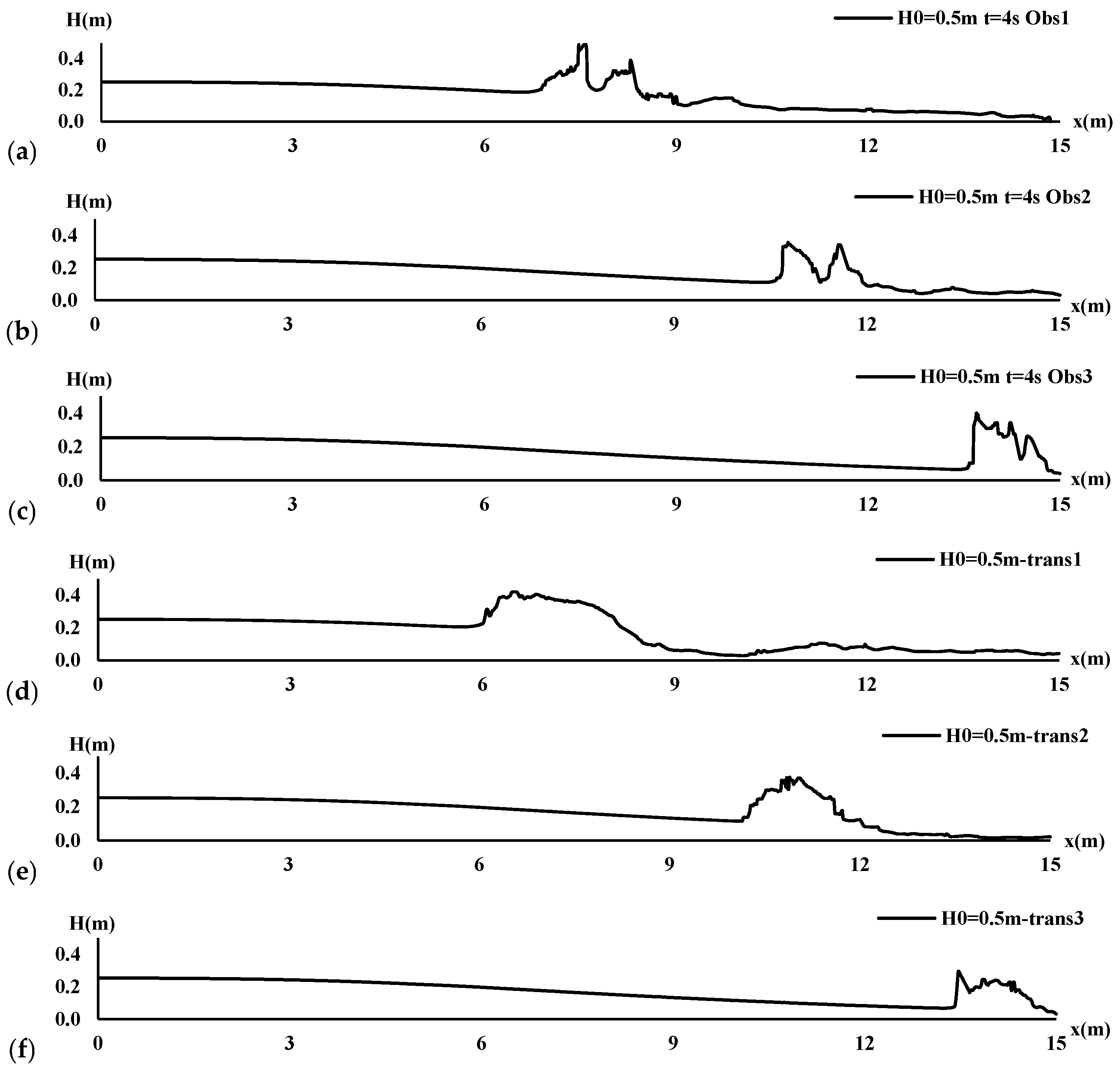
3.2. Free Surface Profile

As the distance of the obstacles from the dam site increased, the flow became more uniform during the dam failure, and the hydraulic jump became less pronounced (Figure 5a,b).

As the obstacles were high and thick, the dam-break flow developed more efficiently around them, resulting in a higher hydraulic jump and more significant energy dissipation (Figure 5a–c). For model S_1,3, no run-up was observed at t = 2 s since the bore had reached the outlet (Figure 5c). The maximum run-up height above the obstacles was 0.47 m and 0.45 m, roughly corresponding to the initial water depth in model S_1,1 at t = 2 s and t = 4 s, respectively. However, the run-up height decreased uniformly in models S_1,2 and S_1,3 with the increasing distance of the obstacles from the dam site (Figure 5a,b). The free surface fluctuations around the obstacles were significant, mainly where the obstacles were close or in the middle distance to the dam site. It was attributed to the dam-break wave’s significant kinetic energy at the early stages. The free surface profile was smoothed with a mild slope before the obstacles from the reservoir’s beginning point to the obstacle location (Figure 5a,b). In contrast, the free surface increased upstream near the contractions due to the formation of the moving hydraulic jump around x = 6 m, 10 m, and 13 m (Figure 5d–f). It differed from the run-up, considering the significant variation in specific energy upstream of the contractions and around the narrowed channel. The moving jump length decreased from around 3 m in Figure 5d to around 1.5 m in Figure 5f by increasing the distance of the contractions from the dam site.

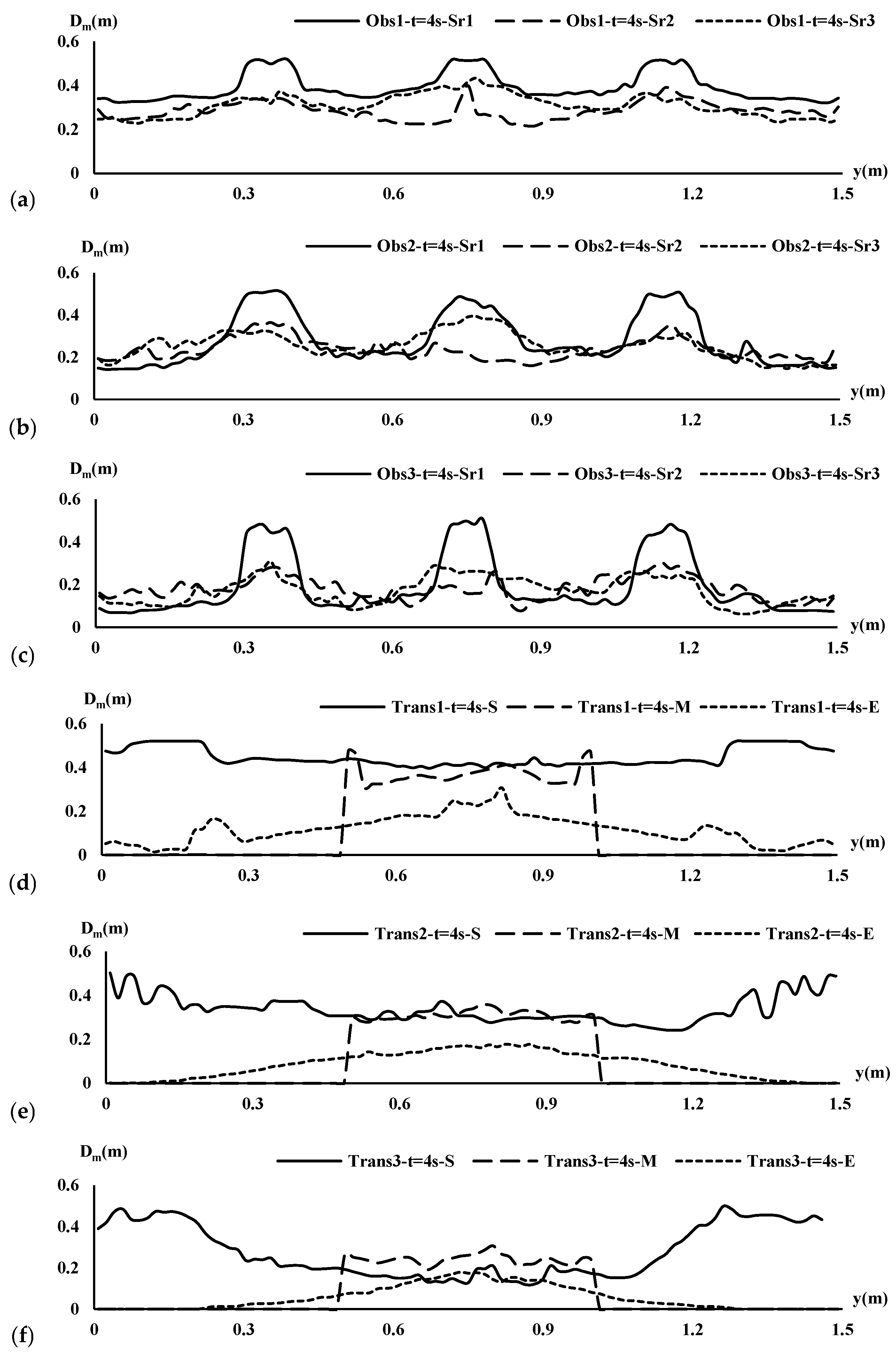
3.3. Flow Depth Fluctuations

The flow depth behind the obstacles fluctuated due to changes in the velocity and pressure of the fluid (Figure 6a–c). The dam-break flow was separated behind the obstacles during wave development and vortices, and air entrapment occurred, forming shadow areas (Figure 6 and Figure 7). The flow depth was negligible or significantly less in these areas than in the surrounding area. Accordingly, the dam-break flow depth decreased substantially in this area. The shadow areas were significantly reduced by increasing the distance of the obstacles from the dam and from S_1,1 to S_1,3. It is worth noting that the downstream channel could become more unstable due to increasing the shear stresses exerted on the channel bottom. The transverse profile of the flow depth had the shape of a high-low. The same variations were observed in the contractions from S_1,4 to S_1,6. In all cases, the maximum flow depth D_m = 0.5 m was observed around the first row of obstacles (Sr1), which could be attributed to the strong run-up over the obstacles. In contrast, the lowest flow depth was observed between obstacles and between obstacles and sidewalls (Figure 6a–f).

The transverse profile of the flow depth had the shape of a high-low. The profiles were also parallel around the obstacles in the second and third rows (Sr1 and Sr2). It could be attributed to the kinetic energy dissipation between the obstacles in the second and third rows after the wave hit the first row of obstacles.

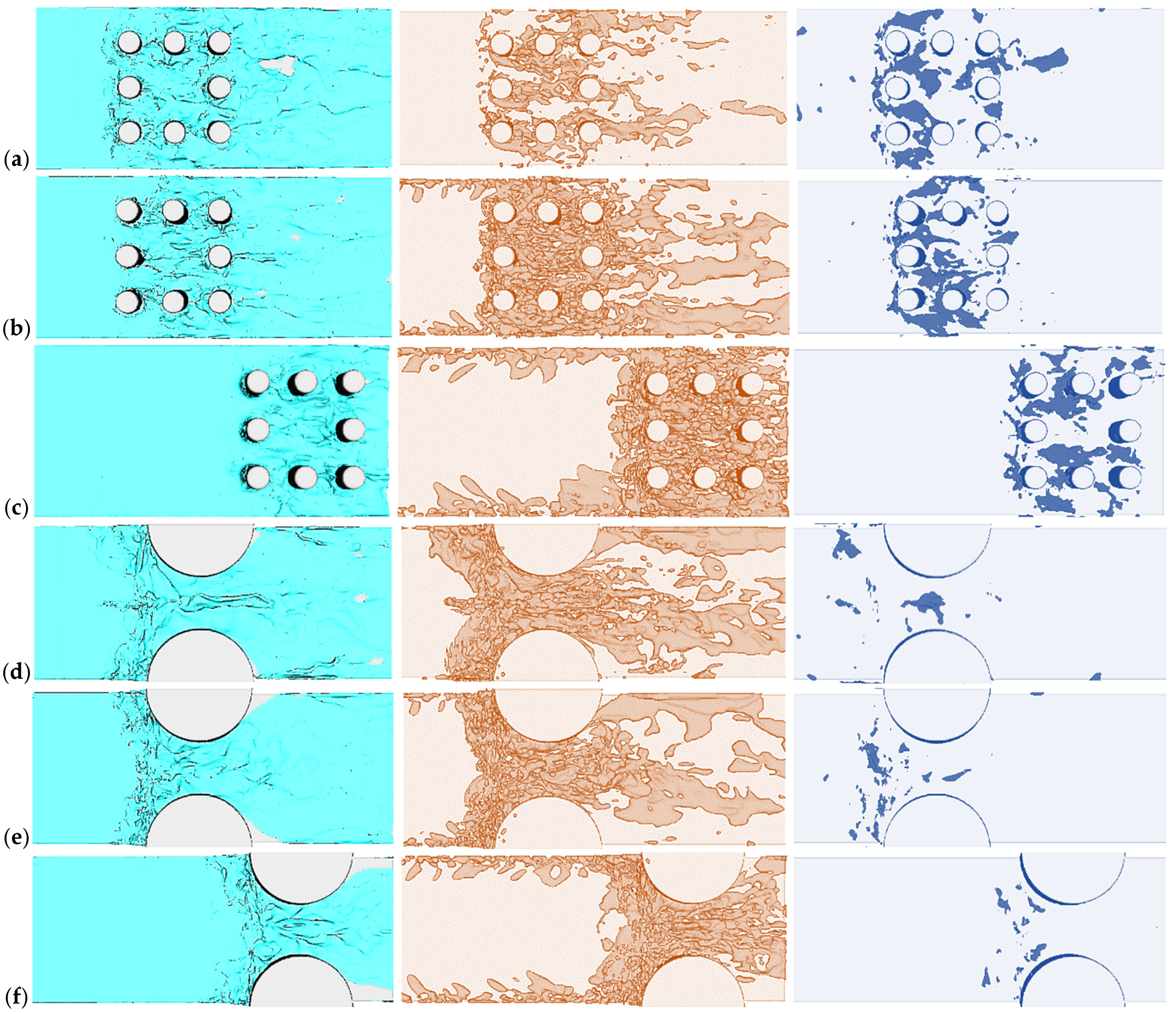
3.4. Turbulence Structures and Air Entrainment

Vorticity is a measure of the rotation or swirl of a fluid, which can form and develop around obstacles in a dam failure as the distance of the obstacles from the dam site increases. The magnitude of the vorticity was directly proportional to the rate of change of the flow velocity. Behind the obstacles, vortex shedding happened because of the flow separation into different paths. The vortices had a cylindrical shape and oscillated periodically. The vortices rotated clockwise or counterclockwise and could persist for an extended period. The intensity of the vortices around the obstacles near the dam was insignificant in the middle phase t = 4 s due to wave attenuation in the presence of prevailing laminar flow in the reservoir (Figure 7a).

The intensity of eddies was significant in the middle of the downstream channel and near the outlet. This was due to the higher flow velocity and developing turbulence structures at t = 4 s (Figure 7b,c). In contrast, the regular shape of vortices was not observed around the contractions. The most intensive vortices were also observed when the vortices were inserted in the middle of the channel for S_1,5. The change in the scale of the vortices and their longitudinal stretching was observed down the contractions (Figure 7d–f).

Air entrapment was the process by which air was trapped in the fluid during the development of a dam break. This occurred around obstacles in the downstream channel as the wave developed over and around them. The free surface stagnated in the low-velocity and low-pressure areas, and the air became trapped in the fluid. The air entrapment resulted in bubbles within the flow. However, the highest density of air bubbles was observed around the first row of obstacles (Figure 7a–c). In contrast, the intensity of vortices was negligible around the contractions. The possible reasons were fewer pressure fluctuations and weak entrapment mechanisms around the contractions. This also could be attributed to the weak flow mixture and increasing the dam-break flow velocity around the contractions (Figure 7d–f).

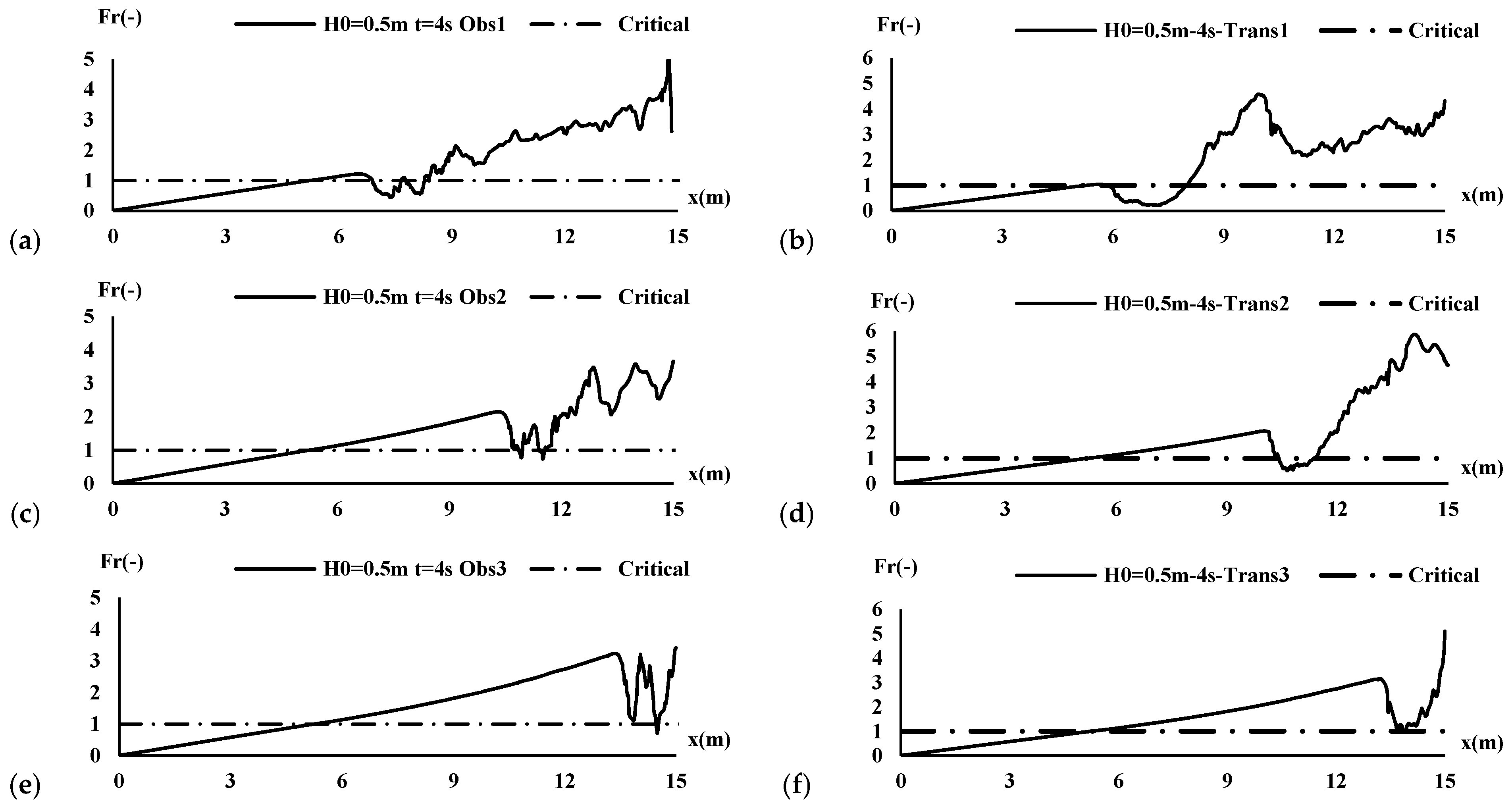
3.5. Dam-Break Flow Regime Variations

The flow regime was transcritical near the dam L_r = x = 5 m and the first row of obstacles. However, after hitting the first row of obstacles, it was displaced to the subcritical between x = 7 and x = 8 m. Some weak hydraulic jumps formed due to a transition from supercritical to subcritical flow behind the obstacles. Then, the Froude number increased, and the flow regime became supercritical due to the rapid evolution of the bore toward the outlet. The maximum Froude number was Fr_max = 5 near the outlet (Figure 8a).

The transcritical flow formed near the dam site x = 5 m in model S_1,2 as in model S_1,1 and near the first row of obstacles at x = 11 m. The transcritical flow formed near the first row of obstacles in model S_1,2 as in model S_1,1. However, before the obstacles, a steady increase in the Froude number was observed from the initial point of the dam x = 0 (left wall) to x = 10.5 m near the first row of obstacles. Then, the Froude number suddenly decreased to Fr = 0.78, and the flow was in a transition phase. After that, the flow velocity increased toward the outlet due to the wave development. The maximum Froud number Fr_max = 3.5 was observed near the outlet, as a free jet formed at this point. (Figure 8c).

As in the previous two cases, a transcritical flow formed near the dam, and a transitional flow formed near the outlet. The maximum Froude number, Fr_max = 3.4, was observed near the channel outlet. Thus, a mixed flow prevailed along the channel. Accordingly, the Froude number decreased with increasing distance between the obstacles and the dam (Figure 8e). The same trends were observed when predicting the Froude number around the contractions. However, the fluctuations of Froude number values along the channel and around the contractions were fewer, especially around the critical points (Figure 8b,d,f).

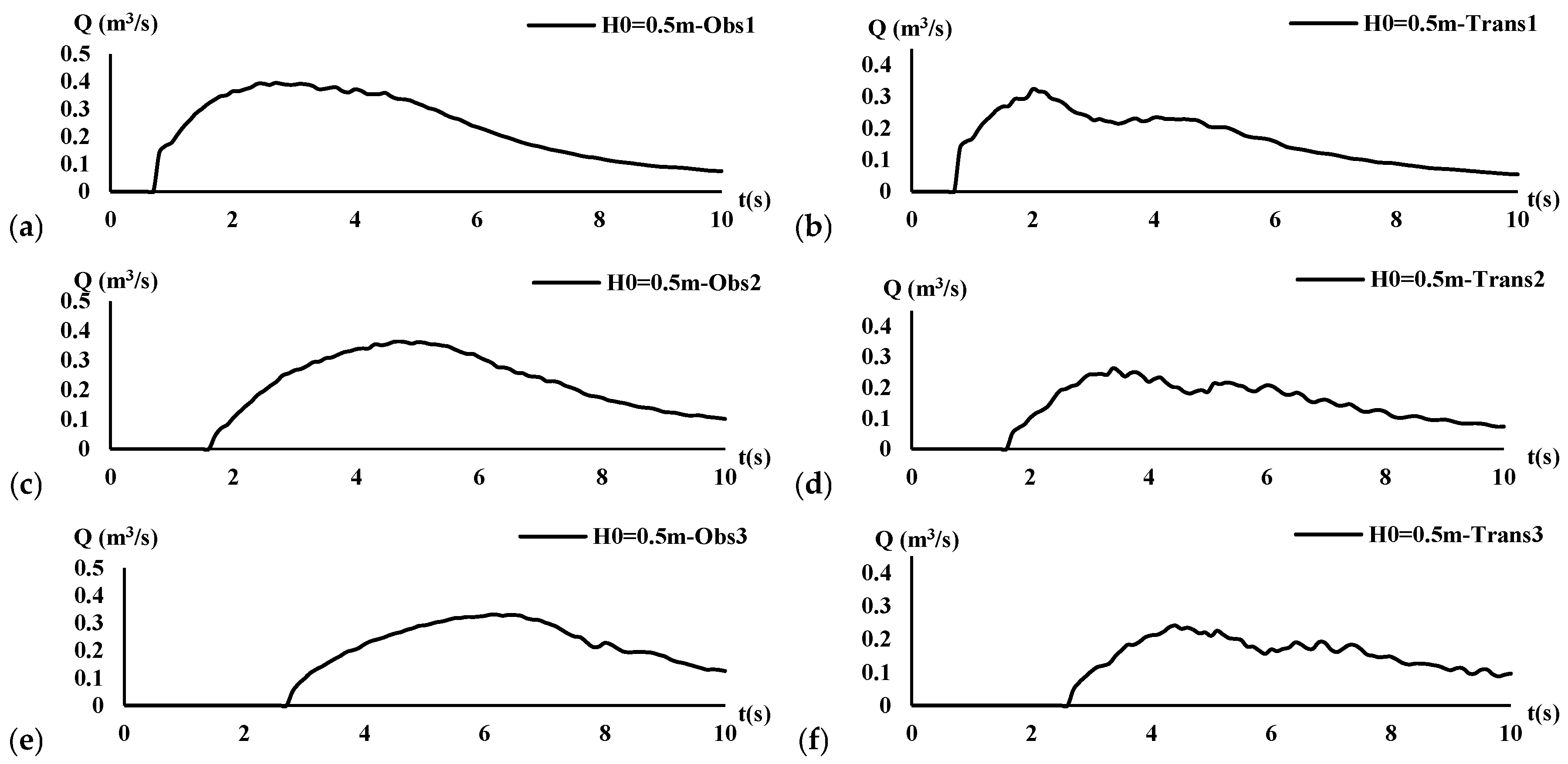
3.6. Inflow Hydrograph in the Downstream Channel

The presence of obstacles in the downstream channel changed the flow direction, causing the wave to break into smaller waves, interacting with the channel bottom, sidewalls, and obstacles in complex ways. The hydraulic jump created by the obstacles near the dam in model S_1,1 affected the inflow hydrograph. This hydraulic jump resulted in a decrease in the height of the free surface and an increase in flow velocity, leading to a rise in inflow. The hydrograph shifted on the time axis from t = 0.7 s to t = 2.6 s, with the rising limb’s length increasing with the distance of the obstacles from the dam (Figure 8a). Accordingly, the peak discharge was reduced from Q_p = 0.4 m³/s in S_1,1 to Q_p = 0.36 m³/s in S_1,2 and Q_p = 0.33 m³/s in S_1,3. Thus, the peak discharge was reduced by increasing the distance of the obstacles from the dam (Figure 8a,c,e). Approximately the same results and peak inflow discharges were predicted for contractions. However, the inflow hydrographs were not smooth like obstacles. The possible reason was the effects of the back-flow toward the reservoir and in the upstream direction. The back-flow development from the constraints toward the reservoir may lead to retentive impacts against the reservoir outflow evolution in the downstream channel (Figure 9b,d,f).

4. Discussion

This study scrutinized the transient dam-break flow and its interaction with downstream obstacles and contractions for different distances of the structures from the dam. The free surface flow evolution and deformations were captured using three-dimensional Navier–Stokes equations coupled with VOF functions. The turbulence characteristics were modeled using LES methods. The results of this study on the effects of obstacles on wave evolution were consistent with those presented in [3,5,9,23]. They showed that the free surface deformations correlated with the downstream structures’ shape, size, and arrangement. The results also showed that the kinetic energy of the dam-break wave and turbulence intensity increased when the obstacles were inserted near the dam [5]. This study also showed that the hydraulic jumps dissipated by increasing the distance of the downstream structures from the dam. This result was similarly reported in a review of dam-breaks in the presence of obstacle research by the authors of [23].

However, despite the previous studies, changing the distance of the downstream structures to the dam was considered a critical factor affecting the wave–structure interactions. It led to significant variations in free surface longitudinal and transverse profiles and fluctuations in flow depth along the channel. Previous studies did not fully address these changes [17,24].

This study also captured the variations in the vortices’ shape, scale, intensity, and air entrainment density around the downstream structures. The results emphasize the difference between obstacles and contractions in developing these phenomena. Accordingly, the intensity of these phenomena was quite different around the downstream structures near the dam from those far from the dam. These phenomena were also scrutinized in previous studies by the authors of [6,10,24]. They correlated the turbulence shedding and air entrapment with the structural impacts and kinetic energy dissipation around these structures.

The numerical results of this study also highlighted the effects of the mesh resolution and turbulence modeling method on model accuracy and performance. These results were consistent with previous numerical dam-break studies [13,33,37,38,39,40]. Indeed, mesh resolution is a critical factor in capturing dam-break wave–structure interactions and the evolution of free surface flow around downstream structures.

Some asymmetries were observed in the free surface profile upstream near the transitions, simulating the dam-break wave evolution around the contractions. The asymmetries along the longitudinal axis could be attributed to numerical and physical factors. While the numerical model was configured with symmetric boundary conditions and refined meshing, small perturbations inherent to the discretization process or solver algorithms may have amplified during the simulation. It was particularly nuanced in regions with complex flow dynamics, such as wake zones and areas of vortex shedding. Additionally, turbulent flows’ inherent unsteady and chaotic nature could lead to slight deviations from perfect symmetry, even under ideal conditions. These asymmetries were not uncommon in numerical studies and have been reported in the literature, especially in highly turbulent transient regimes [29,41,42,43]. Complementary studies need to minimize these effects by conducting additional mesh sensitivity studies and exploring advanced turbulence models to capture better and mitigate such deviations. However, it is essential to note that these localized asymmetries did not significantly impact the overall trends and conclusions of the study.

Previous studies by the authors of [3,9,20] also discussed the development of hydraulic jumps around obstacles and contractions. However, in this study, the characteristics of the hydraulic jump changed by reducing the distance of the downstream structures from the dam. For example, the power and height of the hydraulic jump were more pronounced for the obstacles and contractions near the dam than those far from the dam.

Furthermore, the changes in inflow and outflow hydrographs due to obstacles and wave–structure interactions was reported in previous studies [17,23,24,26]. However, in this study, comparing the shape of the hydrograph for obstacles and contractions highlighted the difference between them in shape and profile fluctuations.

Some limitations of this study that could be addressed in future studies were simplifying the boundary conditions and the geometry of downstream structures, which can be more complex and asymmetrical in real-world frameworks. All structures were considered solid, and the dynamic response of these structures and stress analysis were not included in the results of this study. Accordingly, the dam-break wave was generated as an ideal dam-break problem, while the complexity of the actual dam failure-induced waves was not included in this study.

Future studies can focus on the potential application of the Riemann method for scenarios involving substantial geometric changes or shock-like features. While this study employed the FVM combined with VOF and LES models, which provided robust frameworks for capturing transient flow, these approaches may have limitations in resolving extreme geometric complexities. The Riemann method could complement these techniques in scenarios where shock waves or high-gradient transitions occur. However, the selected methods were sufficient for addressing the research objectives, including evaluating the turbulence intensification, energy dissipation, and wave–structure interactions within an idealized framework. Incorporating the Riemann method could be a valuable avenue for extending this work to more complex, real-world geometries and boundary conditions.

5. Conclusions

This study investigated the transient flow characteristics of dam-break waves interacting with downstream obstacles and contractions under varying distances. The critical findings of this study were as follows:

(1)

The numerical model successfully predicted the evolution of dam-break waves around downstream structures with high accuracy.

(2)

Reducing the distance of obstacles to the dam significantly decreased wave height, kinetic energy, and turbulence intensity, particularly at the early stages of the dam break.

(3)

Hydraulic jumps and transcritical flow regimes were more pronounced around obstacles near the dam.

(4)

The study captured critical phenomena such as air entrainment, vortex shedding, and flow field variations near obstacles, emphasizing their dependency on the proximity of the downstream structures to the dam.

(5)

The inflow hydrograph and peak discharge decreased as the distance of obstacles and contractions from the dam increased, showing the structures’ retentive effects on wave dynamics.

This study has also significant theoretical and practical implications. These findings increase the knowledge of wave–structure interaction due to dam breaks as they have identified the way obstacles and contractions may influence the wave dynamics at various distances from the dam. The comprehensive data about transient flow dynamics, including air entrainment, vortex shedding, and hydraulic jump formation, lay the basic guidelines for designing and optimizing downstream infrastructure concerning resisting extreme flow conditions. These results enable engineers to devise improved strategies for flood risk mitigation against the consequences of dam-break events, especially in high-risk areas with complex hydraulic conditions. Moreover, this numerical approach can be regarded as a reliable framework for other water resources engineering applications, such as urban flood modeling and reservoir outflow management.

Future studies need to be completed on the individual and combined effects of downstream structures’ geometry, number, and material properties. Realistic complications, such as irregular structural layouts, asymmetric boundary conditions, and dynamic responses of downstream structures to wave impacts, would further extend the model’s applicability. Expanding research on sediment transport, debris flow, and erosion at obstructed or channel contractions will also enable a broader understanding of the phenomena. Further, including stress and deformation analyses of structures in the downstream area will help bridge gaps between wave dynamics and structural safety evaluations.

References

1. Haile, T.; Goitom, H.; Degu, A.M.; Grum, B.; Abebe, B.A. Simulation of urban environment flood inundation from potential dam break: Case of Midimar Embankment Dam, Tigray, Northern Ethiopia. Sustain. Water Resour. Manag. 2024, 10, 46. [Google Scholar] [CrossRef]
2. Wang, Y.; Fu, Z.; Cheng, Z.; Xiang, Y.; Chen, J.; Zhang, P.; Yang, X. Uncertainty analysis of dam-break flood risk consequences under the influence of non-structural measures. Int. J. Disaster Risk Reduct. 2024, 102, 104265. [Google Scholar] [CrossRef]
3. Khoshkonesh, A.; Sadeghi, S.; Gohari, S.H.; Oodi, S.; Karimpour, S.; Di Francesco, S. Dam-break flow dynamics over a vegetated channel with and without a drop. Water Resour. Manag. 2023, 613, 128395. [Google Scholar] [CrossRef]
4. Khoshkonesh, A.; Asim, T.; Mishra, R.; Ahmadi Dehrashid, F.; Heidarian, P.; Nsom, B. Study the effect of obstacle arrangements on the dam-break flow. Int. J. Comadem. 2022, 25, 41–50. [Google Scholar]
5. Nazari, R.; Karimi, M. High-resolution hydrodynamic modeling and flood damage assessment in complex urban systems. In XXVIII General Assembly of the International Union of Geodesy and Geophysics (IUGG); German Research Centre for Geosciences: Berlin, Germany, 2023. [Google Scholar]
6. Di Cristo, C.; Greco, M.; Iervolino, M.; Vacca, A. Impact Force of a Geomorphic Dam-Break Wave against an Obstacle: Effects of Sediment Inertia. Water 2021, 13, 232. [Google Scholar] [CrossRef]
7. Giglou, A.N.; Nazari, R.R.; Jazaei, F.; Karimi, M. Numerical analysis of surface hydrogeological water budget to estimate unconfined aquifers recharge. J. Environ. Manag. 2023, 346, 118892. [Google Scholar] [CrossRef]
8. Nazari, R.; Fahad, M.G.R.; Karimi, M.; Eslamian, S. Continuous large-scale simulation models in flood studies. In Flood Handbook; CRC Press: Boca Raton, FL, USA, 2022; pp. 335–350. [Google Scholar]
9. Liu, J.; Song, T.; Mei, C.; Wang, H.; Zhang, D.; Nazli, S. Flood risk zoning of cascade reservoir dam break based on a 1D-2D coupled hydrodynamic model: A case study on the Jinsha-Yalong River. J. Hydrol. 2024, 639, 131555. [Google Scholar] [CrossRef]
10. Qiu, W.; Li, Y.; Zhang, Y.; Wen, L.; Wang, T.; Wang, J.; Sun, X. Numerical investigation on the evolution process of cascade dam-break flood in the downstream earth-rock dam reservoir area based on coupled CFD-DEM. J. Hydrol. 2024, 635, 131162. [Google Scholar] [CrossRef]
11. Zhou, X.; Su, L.; He, X.; Hu, R.; Yuan, H. Experimental investigations of propagation characteristics and wave energy of dam-break waves on wet bed. Ocean Eng. 2024, 301, 117566. [Google Scholar] [CrossRef]
12. Han, Z.; Xie, W.; Yang, F.; Li, Y.; Huang, J.; Li, C.; Chen, G. 3D-SPH-DEM coupling simulation for the large deformation failure process of check dams under debris flow impact incorporating the nonlinear collision-constraint bond model. Eng. Anal. Bound. Elem. 2024, 167, 105877. [Google Scholar] [CrossRef]
13. Biscarini, C.; Di Francesco, S.; Ridolfi, E.; Manciola, P. On the Simulation of Floods in a Narrow Bending Valley: The Malpasset Dam Break Case Study. Water 2016, 8, 545. [Google Scholar] [CrossRef]
14. Akgün, C.; Nas, S.S.; Uslu, A. 2D and 3D Numerical Simulation of Dam-Break Flooding: A Case Study of the Tuzluca Dam, Turkey. Water 2023, 15, 3622. [Google Scholar] [CrossRef]
15. Hien, L.T.T.; Van Chien, N. Investigate Impact Force of Dam-Break Flow against Structures by Both 2D and 3D Numerical Simulations. Water 2021, 13, 344. [Google Scholar] [CrossRef]
16. Biscarini, C.; Di Francesco, S.; Manciola, P. CFD modelling approach for dam break flow studies. Hydrol. Earth Syst. Sci. 2010, 14, 705–718. [Google Scholar] [CrossRef]
17. Khoshkonesh, A.; Nsom, B.; Gohari, S.; Banejad, H. A comprehensive study on dam-break flow over dry and wet beds. Ocean Eng. 2019, 188, 106279. [Google Scholar] [CrossRef]
18. Del Gaudio, A.; La Forgia, G.; Constantinescu, G.; De Paola, F.; Di Cristo, C.; Iervolino, M.; Leopardi, A.; Vacca, A. Modelling the impact of a dam-break wave on a vertical wall. Earth Surf. Process. Landf. 2024, 49, 2080–2095. [Google Scholar] [CrossRef]
19. Kocaman, S.; Özmen-Çagatay, H. The effect of lateral channel contraction on dam break flows: Laboratory experiment. J. Hydrol. 2012, 432, 145–153. [Google Scholar] [CrossRef]
20. Cozzolino, L.; Pepe, V.; Morlando, F.; Cimorelli, L.; D’Aniello, A.; Della Morte, R.; Pianese, D. Exact solution of the dam-break problem for constrictions and obstructions in constant width rectangular channels. J. Hydraul. Eng. 2017, 143, 04017047. [Google Scholar] [CrossRef]
21. Hogg, A.J.; Skevington, E.W. Dam-break reflection. Q. J. Mech. Appl. Math. 2021, 74, 441–465. [Google Scholar] [CrossRef]
22. Valiani, A.; Caleffi, V. Dam break in rectangular channels with different upstream-downstream widths. Adv. Water Resour. 2019, 132, 103389. [Google Scholar] [CrossRef]
23. Dong, Z.; Wang, J.; Vetsch, D.F.; Boes, R.M.; Tan, G. Numerical simulation of air entrainment on stepped spillways. In Proceedings of the E-Proceedings of the 38th IAHR World Congress, Panama City, PA, USA, 1–6 September 2019; p. 1494. [Google Scholar] [CrossRef]
24. Saghi, H.; Lakzian, E. Effects of using obstacles on the dam-break flow based on entropy generation analysis. Eur. Phys. J. Plus 2019, 134, 237. [Google Scholar] [CrossRef]
25. Issakhov, A.; Zhandaulet, Y.; Nogaeva, A. Numerical simulation of dam break flow for various forms of the obstacle by VOF method. Int. J. Multiph. Flow 2018, 109, 191–206. [Google Scholar] [CrossRef]
26. Elong, A.J.; Zhou, L.; Karney, B.; Xue, Z.; Lu, Y. A Comprehensive Numerical Overview of the Performance of Godunov Solutions Using Roe and Rusanov Schemes Applied to Dam-Break Flow. Water 2024, 16, 950. [Google Scholar] [CrossRef]
27. Van Dang, H.; Park, H.; Shin, S.; Ha, T.; Cox, D.T. Numerical modeling and assessment of flood mitigation structures in idealized coastal communities: OpenFOAM simulations for hydrodynamics and pressures on the buildings. Ocean Eng. 2024, 307, 118147. [Google Scholar] [CrossRef]
28. Li, S.; Yang, J.; He, X. Modeling transient flow dynamics around a bluff body using deep learning techniques. Ocean Eng. 2024, 295, 116880. [Google Scholar] [CrossRef]
29. Khoshkonesh, A.; Nsom, B.; Okhravi, S.; Dehrashid, F.A.; Heidarian, P.; DiFrancesco, S. Numerical investigation of dam break flow over erodible beds with diverse substrate level variations. J. Hydrol. Hydromech. 2024, 72, 80–94. [Google Scholar] [CrossRef]
30. Garoosi, F. Numerical Study of Natural Convection Heat Transfer in a Square Cavity with a Cold Obstacle Inside Using the Lagrangian Particle Method. SSRN 2024. [CrossRef]
31. Hirt, C.W.; Nichols, B.D. Volume of fluid (VOF) method for the dynamics of free boundaries. J. Comput. Phys. 1981, 39, 201–225. [Google Scholar] [CrossRef]
32. Lee, H.C.; Wahab, A.K.A. Performance of different turbulence models in predicting flow kinematics around an open offshore intake. SN Appl. Sci. 2019, 1, 1266. [Google Scholar] [CrossRef]
33. Heidarian, P.; Neyshabouri SA, A.S.; Khoshkonesh, A.; Bahmanpouri, F.; Nsom, B.; Eidi, A. Numerical study of flow characteristics and energy dissipation over the slotted roller bucket system. Model. Earth Syst. Environ. 2022, 8, 5337–5351. [Google Scholar] [CrossRef]
34. Boudjelal, S.; Fourar, A.; Massouh, F. Experimental and numerical simulation of free surface flow over an obstacle on a sloped channel. Model. Earth Syst. Environ. 2022, 8, 1025–1033. [Google Scholar] [CrossRef]
35. Lobovský, L.; Botia-Vera, E.; Castellana, F.; Mas-Soler, J.; Souto-Iglesias, A. Experimental investigation of dynamic pressure loads during dam break. J. Fluid Struct. 2014, 48, 407–434. [Google Scholar] [CrossRef]
36. Fraccarollo, L.; Toro, E.F. Experimental and numerical assessment of the shallow water model for two-dimensional dam-break type problems. J. Hydraul. Res. 1995, 33, 843–864. [Google Scholar] [CrossRef]
37. Khoshkonesh, A.; Nazari, R.; Nikoo, M.R.; Karimi, M. Enhancing flood risk assessment in urban areas by integrating hydrodynamic models and machine learning techniques. Sci. Total Environ. 2024, 952, 175859. [Google Scholar] [CrossRef]
38. Pasculli, A. Viscosity Variability Impact on 2D Laminar and Turbulent Poiseuille Velocity Profiles; Characteristic-Based Split (CBS) Stabilization. In Proceedings of the 2018 5th International Conference on Mathematics and Computers in Sciences and Industry (MCSI), Corfù, Greece, 25–27 August 2018. [Google Scholar] [CrossRef]
39. Pasculli, A. CFD-FEM 2D Modelling of a Local Water Flow. Some Numerical Results. Alp. Mediterr. Quat. 2008, 21B, 215–228, ISSN: 2279-7327; SCOPUS: 2-s2.0-84983037047. [Google Scholar]
40. Chung, T.J. Computational Fluid Dynamics; Cambridge University Press: Cambridge, UK, 2006. [Google Scholar]
41. Sun, J.; Lu, L.; Lin, B.; Liu, L. Processes of dike-break induced flows: A combined experimental and numerical model study. Int. J. Sediment Res. 2017, 32, 465–471. [Google Scholar] [CrossRef]
42. Zhang, L.; Xu, W.; Zhang, F.; Zhang, W.; Wei, W.; Zhang, X. Improved general unit hydrograph model for dam-break flood hydrograph. J. Hydrol. 2024, 635, 131216. [Google Scholar] [CrossRef]
43. Zhang, L.; Zhang, F.; Xu, W.; Bo, H.; Zhang, X. An innovative method for measuring the three-dimensional water surface morphology of unsteady flow using light detection and ranging technology. Ocean Eng. 2023, 276, 114079. [Google Scholar] [CrossRef]
Figure 1. Initial and boundary conditions of the idealized city under the effect of the (a) obstacles, (b) contractions, and (c) geometric configuration of modeling case studies. The water within the reservoir is in blue color, while the solid elements, including the channel bed, obstacles, and contractions are shown in red color. The boundary conditions are also listed in arbitrary colors on each mesh plane in figures (a) and (b).
Water 17 00424 g001
Figure 2. Comparison of run time and mean cell size for calibration and validation models.
Water 17 00424 g002
Figure 3. The algorithm of the calibration and validation process in accuracy tests and model optimization.
Water 17 00424 g003
Figure 4. Flow depth plan in models. (a) Obstacles: S1,1, (b) S1,2, and (c) S1,3; (d) contractions: S1,4, (e) S1,5, and (f) S1,6 at t = 4 s. The horizontal and vertical scales are 1.5 and 4, respectively. The color scale inside the shapes presented the flow depth.
Water 17 00424 g004
Figure 5. Free surface profile in models. (a) Obstacles: S1,1, (b) S1,2, and (c) S1,3; (d) contractions: S1,4, (e) S1,5, and (f) S1,6 at t = 4 s.
Water 17 00424 g005
Figure 6. Maximum flow depth profiles in the transverse direction (Dm = Dmax) in models. (a) Obstacles: S1,1, (b) S1,2, and (c) S1,3; (d) contractions: S1,4, (e) S1,5, and (f) S1,6 at t = 4 s.
Water 17 00424 g006
Figure 7. Iso-surface of flow depth, horizontal vorticities, and air entrapment around the obstacles and transitions in models. (a) Obstacles: S1,1, (b) S1,2, and (c) S1,3; (d) contractions: S1,4, (e) S1,5, and (f) S1,6 at t = 4 s.
Water 17 00424 g007
Figure 8. Froude number changes from the beginning of the reservoir to the end of the channel in models. (a) Obstacles: S1,1, (c) S1,2, and (e) S1,3; (b) contractions: S1,4, (d) S1,5, and (f) S1,6 at t = 4 s.
Water 17 00424 g008
Figure 9. Inflow hydrograph of the dam-break flow in the place of downstream structures in models. (a) Obstacles: S1,1, (c) S1,2, and (e) S1,3; (b) contractions: S1,4, (d) S1,5, and (f) S1,6 at t = 4 s.
Water 17 00424 g009