Efficient Naval Surveillance: Addressing Label Noise with Rockafellian Risk Minimization for Water Security

Abstract

This study proposes developing a resilient machine learning algorithm based on neural networks to classify naval images used in surveillance, search, and detection operations in vast coastal and marine environments. Coastal areas critical for water resource management often face challenges such as illegal fishing, trafficking, piracy, and other illicit activities that require robust monitoring systems powered by computer vision. However, real-world datasets in such environments can be compromised by label noise due to random inaccuracies or deliberate adversarial attacks, leading to decreased accuracy in machine learning models. Our innovative approach employs Rockafellian Risk Minimization (RRM) to mitigate the impact of label noise contamination, crucial to maintaining data integrity in water-related security and governance operations. Unlike existing methodologies that rely on extensively cleaned datasets, our two-step process adjusts neural network weights and manipulates nominal probabilities of data points to isolate potential data corruption effectively. This technique reduces dependence on meticulous data cleaning, thereby increasing data processing efficiency in water resources and coastal management. To validate the effectiveness and reliability of the proposed model, we apply RRM in various parameter settings to datasets specific to naval environments and evaluate its classification accuracy against traditional methods. By leveraging the proposed model, we aim to reinforce the robustness of ship detection models, ultimately contributing to developing more reliable automated maritime surveillance systems. Such systems are essential for strengthening governance, security, and water management and curbing illegal activities at sea.

1. Introduction

The field of machine learning (ML) has been expanding rapidly, transforming how machines learn from data to make data-driven predictions and decisions. Within ML, computer vision (CV) has gained prominence as a specialized area that enables machines to interpret visual data at an unprecedented level of complexity. This capability has profound implications across sectors, creating applications in areas like autonomous vehicles, medical diagnostics, security, and military operations. Using sophisticated mathematical models, CV allows for machines to “see” and understand the visual world, creating new pathways for technological advancement and real-world impact.

In the military, CV applications play a critical role in enhancing decision-making processes by improving situational awareness and supporting autonomous systems in dynamic environments. For Brazil, a country with an extensive coastline of approximately 3.6 million square kilometers that spans 200 nautical miles within the Brazilian Exclusive Economic Zone (EEZ) [1], these advancements are essential. The Brazilian Navy (BN) is responsible for safeguarding Brazil’s maritime borders, where challenges such as piracy, smuggling, and illegal pollution persist. The BN launched the Blue Amazon Management System (SisGAAz) to address these threats, leveraging a sophisticated network of satellites, radars, and multi-platform systems for continuous monitoring of Brazil’s jurisdictional waters [2].

Automatic ship detection, an essential component of maritime surveillance, typically depends on meticulously curated datasets. However, gathering and processing high-quality data can be both labor-intensive and time-consuming. This study introduces an innovative approach to improving the robustness of image detection models in naval applications, particularly for binary classification tasks. Building on the Rockafellian relaxation methodology, this approach combines classical convolutional neural networks (CNNs) with stochastic gradient descent (SGD) training, allowing for refined adjustments of nominal probabilities for each image. The Rockafellian method strengthens CNN models by addressing label corruption issues common in ML datasets, which may arise from random inaccuracies or targeted adversarial attacks. This model aims to reinforce data integrity in maritime security operations by reducing dependency on pre-cleaned datasets and improving efficiency in data processing [3,4].

The remainder of this study is organized as follows: Section 2 provides a literature review to support the objectives of this research, offering a detailed summary of relevant concepts, conditions, and practices related to the research aim. Also, Section 2 presents the mathematical formulation and methodologies, discussing the foundational mathematics of the ML algorithms and emphasizing the distinctions between models. Section 3 showcases the results of our three unique methodologies, focusing on model testing accuracy, AUC curve, and computational runtime, with a brief analysis of the outcomes. Section 4 concludes with a summary of the findings and suggestions for future research directions.

2. Materials and Methods

2.1. Background

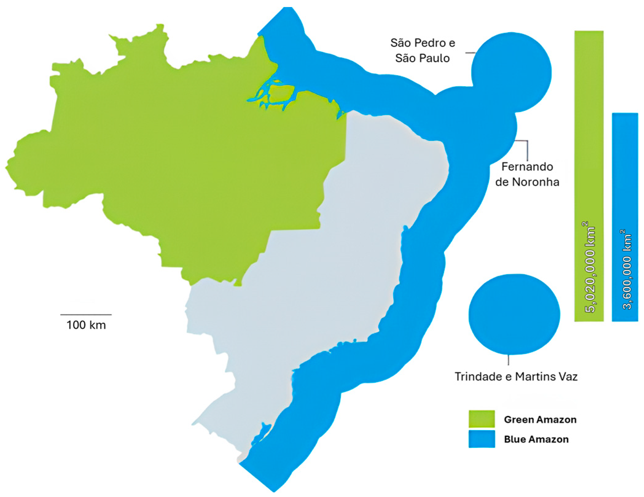
2.1.1. The Blue Amazon

With its 7500 km Atlantic coastline, Brazil has a vested interest in developments concerning the Atlantic Ocean. In 2004, the Brazilian Navy (BN) introduced the term “Blue Amazon”, a vast oceanic area extending from Brazil’s coastline to the edge of its continental shelf, covering the surface, waters, seabed, and subsoil. Registered as a trademark in 2010, the Blue Amazon is a significant region rich in resources like marine biodiversity, minerals, oil, and natural gas [1,2]. Figure 1 compares the dimensions of both Amazons.

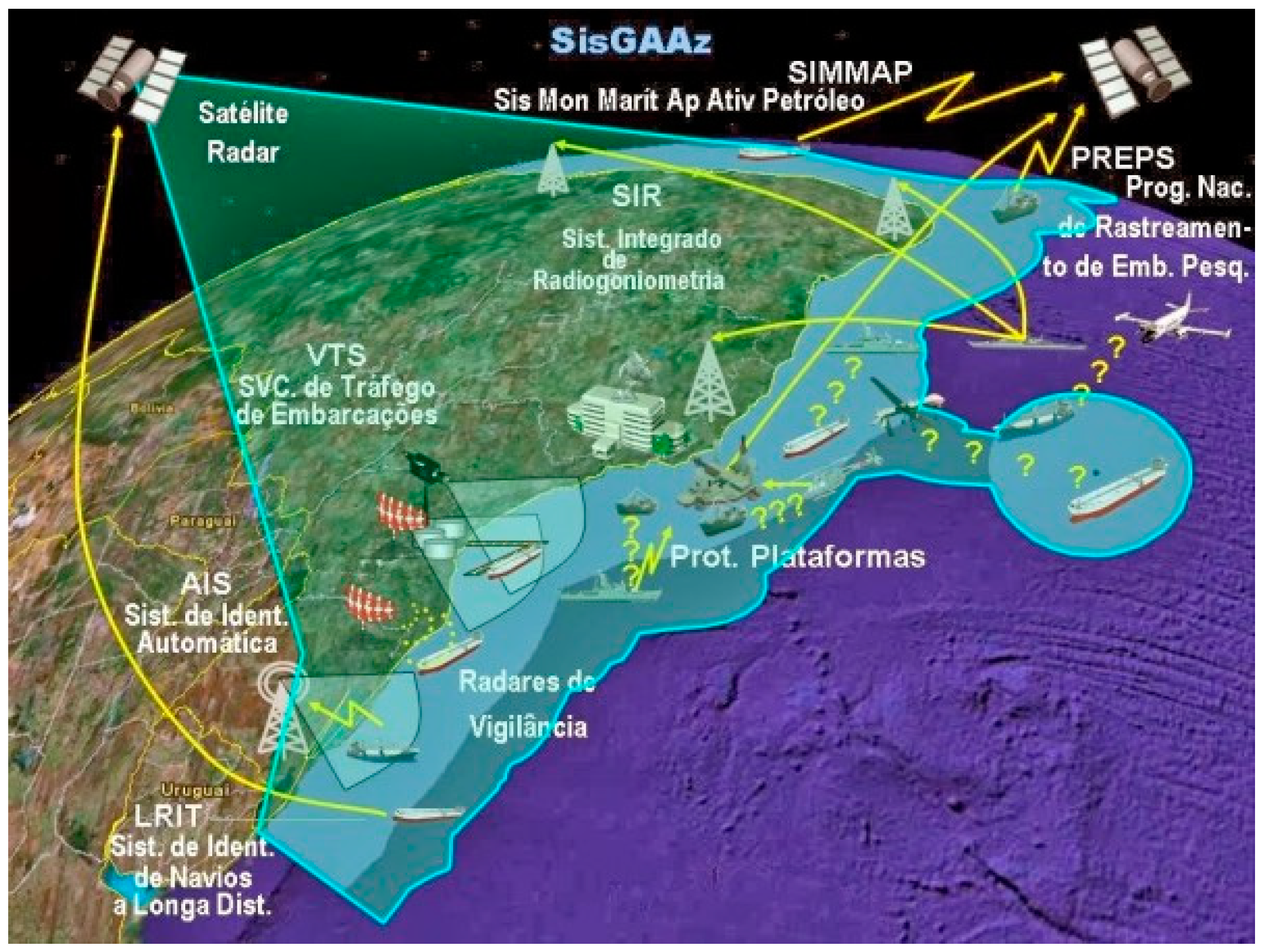
2.1.2. Surveillance System

Protecting the Blue Amazon poses challenges, as insufficient security could lead to criminal activities, including piracy, smuggling, and illegal pollution. To counteract these threats, the BN established the Blue Amazon Management System (SisGAAz), a strategic initiative focused on safeguarding this extensive region [4]. SisGAAz employs satellite technology, multi-platform systems, radars, and sensors for continuous monitoring and management of Brazil’s jurisdictional waters and Search and Rescue (SaR) region, integrating data and decision-making for effective oversight [5,6]. Figure 2 illustrates the SisGAAz system.

2.2. Concepts

2.2.1. Classification

Classification is a key task focused on predicting categorical outcomes or labels by learning boundaries that differentiate classes within the data. Unlike regression, which estimates continuous values, classification assigns each data point to a distinct category, aiding in tasks such as image recognition and spam detection [7,8,9].

Classification tasks are divided into binary and multiclass types based on the number of target categories. This article focuses on binary classification, where data are assigned to one of two categories, typically labeled as 1 and −1 (e.g., predicting purchase likelihood or detecting spam) [10]. In contrast, multiclass classification categorizes data into more than two classes.

2.2.2. Learning and Optimization

Learning and optimization are essential in ML, with learning improving optimization by leveraging past experiences and data patterns. While learning algorithms assume data reflects the real-world problem, optimization algorithms focus on finding the best solution without making such assumptions [11]. The primary goal in ML is to minimize expected generalization error, or risk, which measures performance differences between training and unseen test data [12].

To address this, expected loss minimization is commonly used, calculating average loss across inputs based on the true data distribution. However, with large datasets, this may be computationally impractical. In such cases, empirical risk minimization (ERM) approximates the true distribution using the training data’s empirical distribution, assigning equal probabilities to observed data points [13].

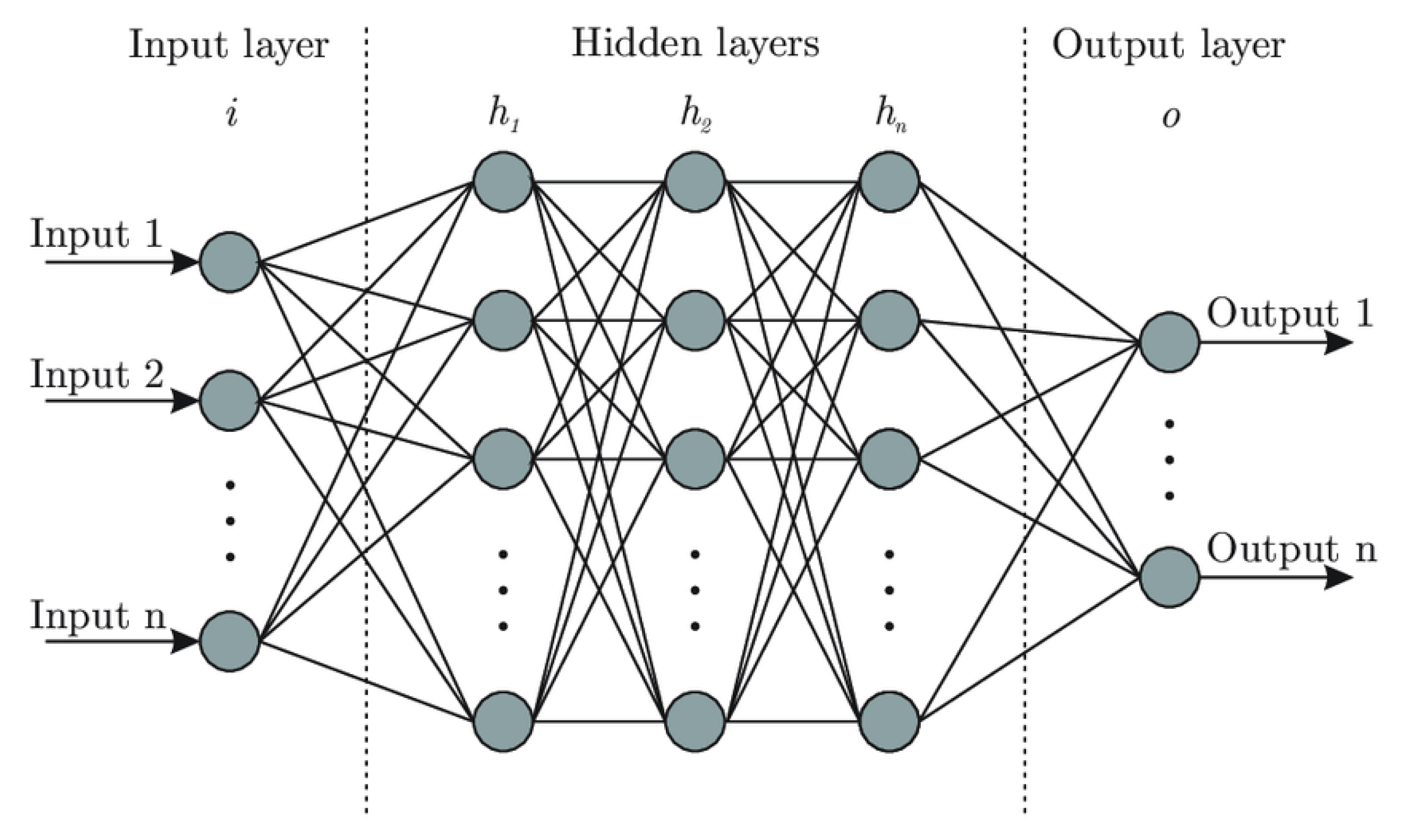
2.2.3. Neural Networks

Neural networks (NNs), a popular type of ML model, are widely used in fields such as image recognition, natural language processing, and pattern recognition. This article primarily focuses on convolutional neural networks (CNNs), a specialized form of NN. Neural networks, also known as artificial neural networks (ANNs), are inspired by the human brain’s structure and consist of three main layers: input, hidden, and output. Figure 3 illustrates this structure.

Neural network layers consist of interconnected neurons that process and learn from data through backpropagation, which calculates error gradients, compares predictions to the target, and adjusts network weights. This iterative process continues until the network minimizes error, achieving accurate predictions. A perceptron neuron, shown in Figure 4, combines weighted inputs, adds a bias, and applies an activation function to generate the final output [14].

Activation functions are essential in training neural networks, as they adjust gradients and introduce nonlinearity, enabling deep networks to learn complex functions [16]. Two widely used activation functions are Rectified Linear Units (ReLU) and Sigmoid.

The ReLU activation function is defined as

$$\mathrm{f}\left(\mathrm{x}\right)=\max (0,\mathrm{x}).$$

(1)

The sigmoid activation function is defined as

$$f\left(x\right)={\displaystyle \frac{1}{(1+\exp \left(-x\right))}}.$$

(2)

Figure 5 shows graphic representations of these activation functions.

Typically, in multilabel classification networks, the final layer utilizes another activation function called softmax. This function converts the real-valued activations into probabilities for different classes [18]; the softmax function is defined as

$$f(x)={\displaystyle \frac{\mathrm{e}\mathrm{x}\mathrm{p} \left(x_i\right)}{{\sum }_{j=1}^K\mathrm{e}\mathrm{x}\mathrm{p} \left(x_j\right)}},$$

(3)

where $x_i$ represents the i-th element of the input vector and ${\sum }_{j=1}^K\mathrm{e}\mathrm{x}\mathrm{p} \left(x_j\right)$ denotes the sum of exponential values over all elements in x. Each probability in the result is in the range 0 to 1, and the sum of the probabilities is 1, representing a valid probability distribution over the K classes.

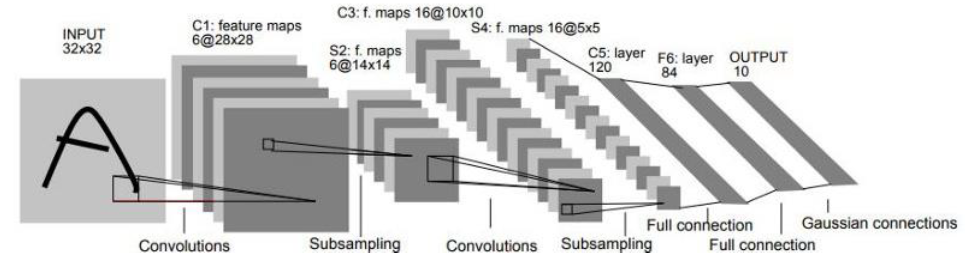
2.2.4. Computer Vision and Convolutional Neural Networks

Computer vision (CV) is a field that develops algorithms to analyze and interpret visual data, enabling machines to perceive and understand the visual world much like human perception [19]. CV applications focus on extracting and categorizing information from images and videos. In this research, we concentrate on images, which are collections of pixels arranged in two dimensions, typically containing color channels such as red, green, and blue (RGB). Each color channel holds specific color intensity values that can be processed to gain insights and make decisions in CV tasks [20].

Convolutional neural networks (CNNs) are the most effective tools in CV for extracting and learning key features from images [21]. CNNs, like traditional neural networks, use weights, biases, and nonlinear functions to produce outputs. However, CNNs uniquely perform convolutions in place of matrix multiplications, using filters or kernels to scan the input image and generate feature maps. Each kernel’s size and stride determine how it navigates the image, influencing output resolution and downsampling when strides greater than one are applied [22].

Pooling layers, typically placed between convolution layers, further downsample feature maps by selecting maximum or average values within a window, reducing spatial dimensions and computational load [23]. After convolutional and pooling operations, the multi-dimensional output is flattened into a one-dimensional array that passes into fully connected (FC) layers, responsible for final predictions. These dense layers function similarly to hidden layers in traditional neural networks, with each neuron fully connected to the previous layer’s neurons [24].

After processing the fully connected layer, the output is passed through a softmax activation function (1.3). This function converts the output values into probabilities for each class. The input is then classified based on the class with the highest probability [25].

2.3. Literature Review

2.3.1. Classification Problem

Early research began with Maron’s Naïve Bayes classifier in 1961, applying Bayes’ theorem with feature independence for classification [26]. In 1967, Cover et al. introduced the k-nearest neighbors (k-NN) algorithm, classifying new data by majority vote among nearby points [27].

In 1986, Quinlan’s Iterative Dichotomiser 3 (ID3) algorithm introduced decision trees to ML, leveraging information gain to recursively split datasets for improved classification [28]. Support Vector Machines (SVMs), introduced by Cortes and Vapnik in 1995, created hyperplanes that separate classes in a way that maximizes margins, proving robust across a variety of data conditions [29]. Ensemble methods like Boosting (Freund and Schapire, 1997) and Random Forests (Breiman, 2001) further improved classification accuracy by combining multiple base models [30,31].

The rise of deep learning transformed classification through neural networks (NNs), with Hinton et al.’s 2006 work on deep belief networks marking a milestone. These deep models excel at identifying complex patterns in high-dimensional data, providing powerful tools for modern classification tasks [32].

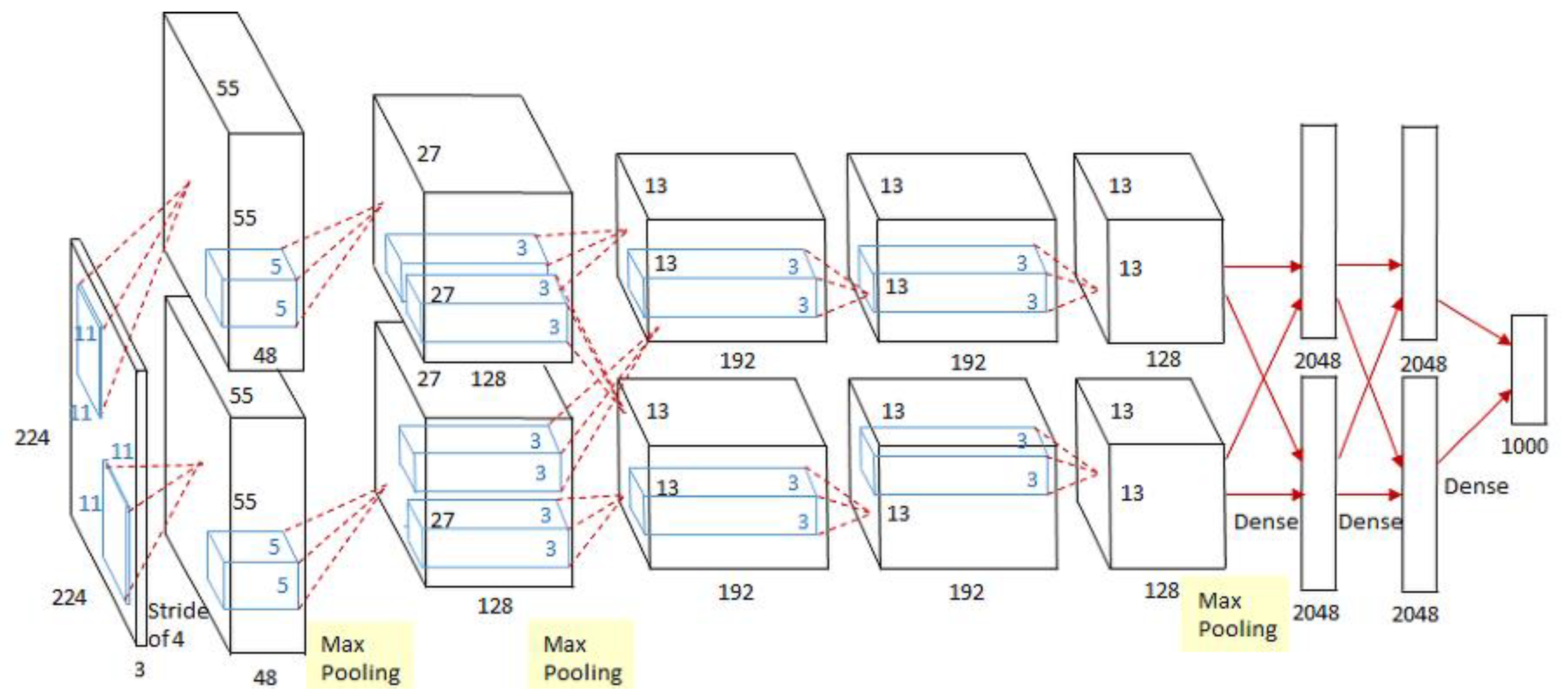
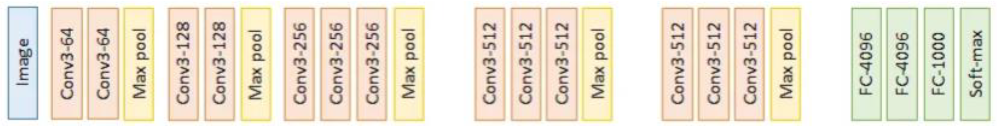
2.3.2. Neural Networks Structures

The concept of computational neurons began with McCulloch et al. in 1943, who modeled binary neurons inspired by brain activity [33]. In 1958, Rosenblatt’s perceptron model expanded on this, calculating weighted sums of inputs and forming the basis of artificial neural networks (ANNs) when combined [34].

Despite initial progress, NN development slowed until 1989, when Rumelhart et al. introduced backpropagation, a method for adjusting weights to minimize errors, enabling more complex applications [35,36]. Convolutional neural networks (CNNs) later emerged to tackle image recognition by extracting features through convolutional layers. LeNet, an early CNN by Yann LeCun in 1998, achieved high accuracy in digit recognition, used by the U.S. Postal Service on the MNIST dataset [37], as presents Figure 6.

The development of CNNs, supported by academia and industry, has included deeper architectures, residual connections, and attention mechanisms, enhanced by GPUs and large datasets like ImageNet. Deep networks faced issues like the vanishing gradient problem, where gradient values become too small to update weights effectively, as highlighted by Glorot et al. in 2010 [38].

Major advancements came from the ImageNet competition, with AlexNet (2012) showing deeper layers improve performance when overfitting is controlled [39], and GoogLeNet (2014) enhancing results by increasing channels per layer [40]. Figure 7 shows the AlexNet architecture.

A key similarity between AlexNet and GoogLeNet is their use of the ReLU activation function (1.1), introduced by Krizhevsky et al. [39], which accelerates training and helps mitigate the vanishing gradient problem. The main innovation in GoogLeNet is its inception module, which captures features at multiple scales using various filter sizes and includes 1 × 1 convolutions to reduce channels, enhancing computational efficiency.

The VGG architecture, developed by Simonyan et al. at the University of Oxford, gained significant recognition in the 2014 ILSVRC for its impressive performance, despite placing second to GoogLeNet [41]. Known for its straightforward design, VGG has had a lasting impact on the deep learning community, with two main variants, VGG-16 and VGG-19, indicating the number of layers in each model. Figure 8 and Figure 9 illustrate the structure of VGG-16 and VGG-19, respectively.

In 2015, He et al. introduced ResNet, a deep learning architecture featuring residual learning through shortcut (or skip) connections [43]. These connections enable gradients to bypass certain layers, making it feasible to train much deeper networks than before. ResNet’s innovative design, with residual blocks to capture complex features, quickly gained popularity and won the 2015 ILSVRC classification task [44].

VGG and ResNet share a notable similarity in their depth, with VGG reaching up to 19 layers and ResNet extending this concept to 152 layers. However, they differ in their approaches to addressing the vanishing gradient problem. While VGG suffers from this issue due to its uniform structure, ResNet mitigates it with residual learning via skip connections, allowing for gradients to bypass certain layers [45,46].

Additionally, VGG has a straightforward architecture of 3 × 3 convolutions and 2 × 2 pooling, while ResNet’s design is more complex due to its use of residual blocks. Together, these architectures represent advances achieved through both theoretical and empirical exploration in CNN development.

2.3.3. Maritime Computer Vision

Computer vision (CV) aims to replicate and enhance human visual interpretation capabilities, bringing significant advancements to maritime operations. Traditional navigation tools—such as vessel traffic services (VTSs), radar, and automatic identification systems (AISs)—have been foundational in maritime monitoring but face limitations. Research by Yassir et al. highlighted that camera surveillance systems can bridge these gaps, enhancing threat prediction and mitigating illegal activities [47,48,49,50].

The integration of CNN-based CV has significantly advanced maritime image interpretation, as shown in studies using specialized datasets for target classification. One study achieved a 94% success rate in classifying marine targets using a CNN with data augmentation [51]. Another, by Gallego et al., utilized the MASATI dataset and transfer learning, boosting accuracy to 99.76% with pre-trained models like VGG and ResNet [52]. Fang et al. further enhanced detection of small targets using CNNs with infrared imaging, demonstrating improvements in robustness and accuracy [53].

Recent developments in UAVs and sensor technology, paired with increased computational power, have propelled CV applications in maritime surveillance. UAVs equipped with CV have shown success in object detection, utilizing models like YOLO for real-time performance [54]. Lo et al. and Lygouras et al. demonstrated YOLO’s efficiency in UAV-based surveillance, showing the potential of deep learning for dynamic object tracking and search-and-rescue (SAR) tasks [55,56,57,58].

Reflecting this growing importance, the Maritime Computer Vision (MaCVi) workshop debuted in 2023, emphasizing the rising role of CV in maritime applications [59].

2.3.4. Label Noise

To develop high-performance deep learning models, experts employ various techniques, including preprocessing, data augmentation, and transfer learning from established architectures. However, a common issue in real-world data is label noise, which can significantly impact model outputs. Label noise, where labels are incorrectly assigned due to errors or deliberate alterations, affects real-world datasets with an estimated 8–38.5% corruption rate [60,61]. Errors arise from random noise during data collection or labeling, and intentional data poisoning, where attackers manipulate data to degrade model performance [62,63].

Researchers have proposed various methods to mitigate label noise’s effects without major structural changes. For instance, Ren et al. introduced a meta-learning algorithm that weights training samples by gradient orientation to improve performance under noisy labels [64]. Thulasidasan’s deep abstaining classifier (DAC) selectively ignores confusing samples during training, enhancing robustness [65]. Chen et al. implemented a hierarchical structure to adapt loss based on noise ratios, bolstering model resilience [66]. Narasimhan et al. combined learning-to-reject (L2R) with out-of-distribution (OOD) detection to handle outliers and complex samples, allowing for the model to abstain from such instances effectively [67,68,69,70].

This study builds on Royset et al.’s Rockafellian relaxation [25], which optimizes models by allowing flexibility in decision-making under label noise, enhancing stability. Rockafellian relaxation analyzes the sensitivity of assumptions and parameters, supporting robust optimization [71]. We apply this framework to improve the reliability of computer vision (CV) in maritime contexts, focusing on label accuracy and model stability, aiming to contribute to resilient deep learning models in noisy environments.

2.4. Rockafellian Risk Minimization

This section develops Rockafellian relaxation in the context of ML, leading to Rockafellian Risk Minimization (RRM) as a means for training in settings with corrupt data. We contrast the approach with ERM and discuss computational aspects.

2.4.1. Formulation

In a labeled set ${\{x}_j{,y}_j,j=1,\dots ,n\}$ of images, $x_j$ specifies the attributes of each pixel in the j-th image and $y_j$ is the corresponding label we seek to determine a parameter vector w in a neural network (NN) so that the prediction corresponds to the label. Considering two labels, −1 and 1, and $g_w\left(x_j\right)$ as the NN prediction for the j-th image’s label, the binary cross-entropy loss function (Equation (4)) is used to determine the vector w that minimizes the loss:

$$f_j\left(w\right)=\left\{\begin{array}{c}-\ln g_w\left(x_j\right) if y_j=1\\ -\ln \left(1-g_w\left(x_j\right)\right) if y_j=-1.\end{array}\right.$$

(4)

Classical ERM then amounts to solving the optimization problem:

$$\underset{w\in {\mathbb{R}}^d}{\mathit{minimize}}{\sum }_{j=1}^n p_j f_j\left(w\right),$$

(5)

where $p_j$ = $1/n$ typically but the data points can also be weighted differently.

In many applications, data corruption can occur due to various reasons such as data collection and labelling entry errors, or even adversarial attacks intended to poison the training data and disrupt the system. As pointed out by Royset et al. [25], and elaborated in section D of chapter II, an NN that has been trained using ERM may not perform well if the training data are corrupted. This observation provides a strong motivation for RRM, an adaptive method to identify and remove corrupted data points, hence improving the overall performance and reliability of the model [72].

RRM leverages auxiliary decision variables ${ u}_1, \dots , { u}_n$, to adjust the probability associated with each data point. This leads to the formulation

$$\underset{w\in {\mathbb{R}}^d,u\in U}{\mathrm{minimize}}{\sum }_{j=1}^n\left(\left.{(p}_j+u_j)f_j\left(w\right)+\theta \left|u_j\right|\right)\right.,$$

(6)

where $\theta$ represents a penalty parameter, u is a perturbation vector with n dimensions that alters the nominal probability vector $p$, and the set

$$U=\left\{u\in {\mathbb{R}}^n\left|u_j\ge -p_j,{\sum }_{j=1}^n{u}_j=0\right.\right\}.$$

(7)

We adjust the probability associated with each data point by adding $u_j$ to $p_j$. To identify corrupted data points, we optimize $u$ based on their calculated loss with the goal of reducing the probability that affects $f_j\left(w\right)$ to zero. This effectively eliminates the data point from being considered in the training process.

2.4.2. Training Algorithm

The RRM method consists of the usage of an Alternating Direction Heuristic based on Linear Programming (ADH-LP), which alternates between optimizing different sets of variables while keeping the others fixed, hence the name “alternating direction”. This strategy begins by optimizing w, which adjusts the neural network weights. Subsequently, we optimize u to modify each data point’s probability, isolating and discarding potential data corruption. The model is refined progressively in each cycle until it reaches the number of iterations defined by the user. Linear programming optimizes u through an objective function with linear constraints, and the parameter is the step size μ ∈ (0,1] that updates u at each iteration i. We note that components of $u^i$ sum to zero and are always greater than $-p_j$. The details of the algorithm are given next.

Alternating Direction Heuristic (ADH-LP)

Data. Number of epochs $\kappa$, number of iterations $\tau$, initial weights $w^0$, and stepsize $\mu .$

Step 0. Set iteration counter $i=1, p^1=p, u^1=0.$

Step 1. Starting from $w^{i-1}$, apply SGD-type algorithm for $\kappa$ epochs to the problem

$$\underset{w\in {\mathbb{R}}^d}{\mathrm{minimize}}{\sum }_{j=1}^n{p}_j^i{f}_j\left(w\right).$$

(8)

Let $w^i$ be resulting solution.

Step 2. Select $u^{i+1}$ for application in the LP based on $w^i$ and $u^i$.

Step 3. Solve the linear optimization problem

$$\underset{u\in \mathit{U} ,\mathit{v}\in {\mathbb{R}}^n}{\mathrm{minimize}}{\sum }_{j=1}^n\left(u_j\right.\left.f_j\left(w^i\right)+\theta v_j\right) {s.t.u}_j\le v_j, {-u}_j\le v_j, j=1,\dots , n.$$

Let ($u^{*},v^{*})$ be a minimizer.

Step 4. Set $u^{i+1}=\mu u^{\mathrm{*}}+\left(1-\mu \right)u^i$. Go to Step 3.

Step 5. If $i<\tau ,$ set $p^{i+1}=p+u^{i+1}$, replace $i$ by $i$ + 1, and back to Step 1.

Else, stop.

3. Results

In this section, we delve into the model’s results, beginning with a discussion on datasets, data preprocessing, optimizers, and network structures. We then present the results achieved by our ERM and RRM models both without label contamination and under varying levels of label contamination in training data. Following this, we analyze the behavior of our perturbation vector values in specific cases. Finally, we evaluate the adaptability and robustness of RRM compared to ERM across different contamination levels.

We utilize two datasets: the Airbus Ship Detection (AIRBUS) [73] and Maritime Satellite Imagery (MASATI) [52] datasets.

Each dataset is examined in its own subsection, detailing unique characteristics and specific challenges. In both, we consider an environment without label contamination and another where label contamination in the training set is gradually increased, starting from 10%, 20%, 30%, and 40% by randomly swapping training example labels. Higher contamination levels of 50% and 60% were tested, but the CNNs struggled to learn patterns at these levels.

The CNN topology used in this study was selected through a combination of empirical experimentation and systematic hyperparameter tuning to balance performance and computational efficiency. The primary focus of this research is not the CNN architecture itself but the application of the RRM methodology to mitigate label noise in maritime datasets. However, to ensure that the CNN was capable of effectively extracting relevant features, the spatial resolution of the input images was carefully considered. Both datasets used in this study—MASATI and Airbus Ship Detection—contain RGB images resized to the same dimensions, ensuring consistency in preprocessing and compatibility with a single CNN topology. This standardization eliminated the need to design separate architectures for each dataset.

The choice of resizing was guided by the need to maintain visual clarity of small vessels, which are critical targets for detection. The resolution was adjusted to a level where ships could still be visually distinguishable to the human eye, preserving key spatial features while reducing computational demands. Although the datasets originally differ in resolution—768 × 768 pixels for AIRBUS and 512 × 512 pixels for MASATI—resizing them to a common input dimension ensured that the CNN could process both datasets effectively without requiring topology modifications. This approach provided a consistent framework for evaluating the RRM methodology across datasets with varying characteristics.

The relationship between spatial resolution and CNN topology is particularly relevant for detecting ships of varying sizes. High-resolution images allow for the identification of smaller ships, while maintaining a balance between resolution and computational efficiency ensures practical applicability in real-world scenarios. By adopting a standardized preprocessing approach and ensuring that the resized resolution was sufficient to retain critical features, the CNN topology was made robust and generalizable. This design decision highlights the emphasis on evaluating the RRM’s effectiveness, while ensuring the CNN’s ability to process maritime data with diverse spatial resolutions.

Our experiments are conducted using Tensorflow version 2.11.0. For w-optimization in the first phase of the ADH process, we employ two NN optimizers: Adam [74] and SGD [75]. Adam is set with a learning rate of $1.0·{10}^{-3}$, while SGD uses a learning rate of 0.1 for the AIRBUS dataset and 0.02 for the MASATI dataset, with a momentum of 0.9 for both datasets. All experiments run on a single Nvidia Tesla V100 GPU with 32 GB of memory.

For u-optimization in the second phase of the ADH process, we use the ADH-LP algorithm, implemented with Pyomo version 6.4.0 and the CPLEX solver.

We investigate various network architectures, learning rates, and other hyperparameters, though our goal is not to enhance performance by altering network architecture. Instead, we aim to show that an RRM approach can offer benefits over an ERM approach regardless of network configuration. For comparison, we select two network configurations. Both CNNs take resized 128 × 128 × 3 images as input, with ReLU activation in hidden layers and two softmax-activated output units for binary classification. The Adam-optimized CNN has 2,228,002 trainable parameters, while the SGD-optimized CNN has 8,409,026.

Table 1. Description of the CNN used for Adam.

#	Layer	Filters	Kernel Size	Output Size	# Parameters
1	Convolution	16	3 × 3	128 × 128 × 16	448
	Max-Pooling		2 × 2	64 × 64 × 16
2	Convolution	32	3 × 3	64 × 64 × 32	4640
	Max-Pooling		2 × 2	32 × 32 × 32
3	Convolution	64	3 × 3	32 × 32 × 64	18,496
	Max-Pooling		2 × 2	16 × 16 × 64
4	Convolution	128	3 × 3	16 × 16 × 128	73,856
	Max-Pooling		2 × 2	8 × 8 × 128
5	Fully connected	256		1 × 256	2,097,408
6	Fully connected	128		1 × 128	32,896
7	Softmax (Output)	2		1 × 2	258

and

Table 2. Description of the CNN used for SGD.

#	Layer	Filters	Kernel Size	Output Size	# Parameters
1	Convolution	32	3 × 3	128 × 128 × 32	896
2	Batch Normalization Activation				128
3	Max-Pooling		2 × 2	64 × 64 × 32	-
4	Convolution Activation	64	3 × 3	64 × 64 × 64	18,496
	Max-Pooling		2 × 2	32 × 32 × 64
5	Fully-connected	128		1 × 128	8,388,736
6	Batch Normalization Activation				512
7	Softmax (Output)	2		1 × 2	258

detail the CNN structures used with each optimizer. Both networks use binary cross-entropy as the loss function.

After establishing a baseline model with ERM, we apply the RRM algorithm ADH-LP using the same network configurations.

For ERM, we set the number of epochs κ = 500. For RRM algorithm, we establish κ = 10 and iterations τ = 50, which guarantees that all heuristic runs will include 500 epochs. The ADH-LP uses the default step size parameter µ = 0.5. Concerning the penalty parameter θ in both ERM and RRM, we show 5 different levels of θ to evaluate their performance in the u-optimization across the values of θ ∈ {0.15, 0.20, 0.25, 0.30, 0.35}.

Table 3. Parameters for ERM and RRM.

	Parameters
Algorithm	Epochs (κ)	Iterations (τ)	Stepsize (µ)	Penalty (θ)
ERM	500	1	-	-
RRM(ADH-LP)	10	50	0.5	0.15, 0.20, 0.25, 0.30, 0.35

summarizes the parameters described.

To compare results, we ensure that the random seed is the same at two specific times for all runs: when we divide the data into training and testing sets and when we execute closed-set contamination through label swapping.

Table 4. Computational time of algorithms.

	Dataset
	MASATI				AIRBUS
	CNN Optimizer				CNN Optimizer
	Adam		SGD		Adam		SGD
Optimization phase	w	u	w	u	w	u	w	u
Algorithm	Total runtime in seconds over optimization phases
ERM	500	-	1400	-	22,500	-	68,500	-
RRM (ADH-LP)	500	600	1400	600	22,500	1000	68,500	1000

summarizes the algorithm runtimes over 500 epochs, separating the time used for the w-optimization and for u-optimization processes in both datasets.

There are noticeable differences between the MASATI and AIRBUS datasets and the Adam and SGD optimizers. When using the Adam optimizer on the MASATI dataset, the ADH-LP method takes 1100 s. However, if we switch to the SGD optimizer, ADH-LP takes 2000 s. Looking at the AIRBUS dataset, with the Adam optimizer, RRM with ADH-LP takes 23,500 s to complete. Under the SGD optimizer, ADH-LP requires 69,500 s. It is worth noting that the ADH-LP method takes longer in the u-optimization process, especially in the larger AIRBUS dataset.

3.1. MASATI Dataset

The MASATI dataset [52] provides a rich collection of maritime scenes captured through optical aerial imagery in the visible spectrum. Designed to evaluate ship detection and classification methods, MASATI stands out for its representation of dynamic marine environments. Each image in the dataset is a color (RGB) image with a fixed resolution of 512 × 512 pixels, stored in the PNG format, which ensures lossless image quality and preserves visual details critical for machine learning applications. The dataset incorporates significant variability in weather, lighting, and the presence of multiple targets, making it a challenging yet valuable resource for robust model evaluation.

The full MASATI dataset consists of 7389 labeled images distributed across seven distinct classes: coast, land, ship, sea, coast–ship, multi, and detail. These classes are designed to represent the diverse maritime conditions and scenes captured within the dataset, ranging from open water to coastlines and complex multi-target scenarios. For this study, however, the dataset was adapted to a binary classification problem. Specifically, two classes were selected: “ship”, comprising 1027 images, and “sea”, containing 1022 images. This reduced the dataset to a total of 2049 images, enabling a focused investigation into the presence or absence of ships in maritime environments.

Despite its relatively small size, this binary subset of the MASATI dataset offers a unique opportunity to assess the robustness and adaptability of ship detection algorithms. The limited number of images emphasizes the need for efficient model training and testing, ensuring that the results are not overly reliant on large-scale data. This makes MASATI particularly valuable for evaluating the performance of algorithms in scenarios where data availability is constrained, a common challenge in real-world maritime applications.

Furthermore, the inclusion of challenging environmental factors, such as varying weather conditions, illumination changes, and the presence of multiple targets within a single image, highlights the dataset’s complexity. These characteristics ensure that any proposed method must be versatile and robust to deliver accurate results. Figure 10 of the study illustrates some example images from the dataset, showcasing the diversity and dynamic nature of the scenes captured.

3.1.1. Accuracy Results with MASATI

In this section, we show our results in the MASATI dataset, explicitly focusing on the accuracy score, which indicates how effectively our models can classify images within the test set. Along with presenting the results, we also provide a thorough analysis to interpret the observed performance.

In MASATI, the train/test split is achieved using a 90/10 proportion, which results in 1844 images in the training set and 205 in the test set.

The final test accuracy results for ERM and RRM with ADH-LP using Adam optimizer are shown in

Table 5. Final test accuracy in MASATI for ERM and RRM (ADH-LP/Adam).

	Corrupted Training Data Percentage
Method	40%	30%	20%	10%	0%
ERM	0.624	0.653	0.785	0.858	0.941
RRM (μ = 0.5)
θ = 0.15	0.624	0.668	0.800	0.863	0.951
θ = 0.20	0.609	0.726	0.848	0.878	0.931
θ = 0.25	0.668	0.682	0.814	0.863	0.941
θ = 0.30	0.604	0.702	0.804	0.843	0.926
θ = 0.35	0.614	0.692	0.756	0.834	0.921

Note: The values highlighted in gray represent the cases where RRM outperform or match ERM.

at various levels of corruption.

The RRM method exhibits performance at par or even superior to ERM at various levels of data corruption, especially for specific penalty values. Remarkably, when the values of 0.15, 0.20, and 0.25 are chosen for θ, they yield the best overall performance. For example, θ = 0.15 performs exceptionally well at lower corruption levels, θ = 0.20 outperforms all other θ values at a 20% corruption level, and θ = 0.25 performs best at a 30% corruption level.

The performance difference is relatively minimal in scenarios where the RRM method does not surpass ERM. This finding implies that even with non-optimal selections of θ, the RRM method can deliver performance nearly equivalent to ERM. It accentuates the versatility of the RRM method as a promising alternative to ERM, especially in environments fraught with corrupted data.

The topology of the CNN used in this study was primarily selected based on empirical results obtained during the experimentation phase and through a systematic hyperparameter search, ensuring a balance between performance and computational efficiency. Although the primary focus of this research is the mathematical model for mitigating errors in noisy datasets rather than the CNN architecture itself, the network design aimed to effectively capture image patterns, including small vessels. To achieve this, the spatial resolution of the images from both the MASATI and AIRBUS datasets was uniformly resized to a level where small vessels could still be visually distinguishable to the human eye. This resizing criterion ensured that critical visual features were preserved during preprocessing.

Furthermore, as both datasets were resized to the same dimensions before being fed into the CNN, there was no need to adapt the network topology to account for differences in the original resolutions. This standardized approach simplified implementation and allowed for a focused evaluation of the RRM methodology under varying levels of label noise. The selected CNN topology and preprocessing pipeline proved sufficient to support the primary objective of this study: assessing the robustness of the proposed RRM framework in scenarios with corrupted datasets.

The results of the experimentation phase suggest that a set of θ ∈ {0.15, 0.20, 0.25} provides an optimal balance in modulating the penalty for model complexity versus the fit to training data. This balance contributes to superior generalization of the test data, particularly at intermediate corruption levels.

Now, turning to the SGD optimizer,

Table 6. Final test accuracy in MASATI for ERM and RRM (ADH-LP/SGD).

	Corrupted Training Data Percentage
Method	40%	30%	20%	10%	0%
ERM	0.556	0.546	0.581	0.663	0.648
RRM (μ = 0.5)
θ = 0.15	0.604	0.648	0.648	0.639	0.634
θ = 0.20	0.663	0.692	0.648	0.648	0.609
θ = 0.25	0.639	0.687	0.658	0.629	0.614
θ = 0.30	0.668	0.585	0.600	0.643	0.634
θ = 0.35	0.624	0.556	0.639	0.648	0.653

Note: The values highlighted in gray represent the cases where RRM outperforms or matches ERM.

displays the final test accuracy results for ERM and RRM in ADH-LP at various levels of corruption.

From Table 6, the RRM method, when compared with ERM, delivers better or comparable performance at different levels of data corruption.

Examining the selection of the θ ∈ {0.20, 0.25, 0.30}, we observe that these selections yield the highest accuracies across the range of data corruption levels.

At a 40% corruption level, the RRM outperforms the ERM method. For θ = 0.20, the accuracy improvement is a substantial 10.7%. Similarly, for θ = 0.30, the performance is enhanced by 11.2% compared to ERM. When faced with 30%, the accuracy improvement for θ = 0.20 over ERM is an impressive 14.6%, the highest observed in this dataset. In the 20% corruption level, the RRM with a θ = 0.25 exhibits a promising 7.7% improvement in accuracy over the ERM.

Interestingly, at lower corruption levels of 10% and 0%, the performance of RRM remains comparable to ERM. This reveals the versatility of the RRM method, maintaining robust performance even as the corruption level diminishes.

The superior performance of RRM at higher corruption levels (20%, 30%, and 40%) across all θ values, combined with its comparable performance at lower corruption levels, indicates its resilience.

3.1.2. U-Optimization Analysis with MASATI

In the following section, we aim to examine the u-vector behavior in some MASATI cases. We show the dynamic evolution of the perturbation vector values across the iterative steps of the RRM algorithm and how it influences performance and resilience, thereby illustrating its crucial role within this methodology.

The u-vector helps improve the model’s performance by adjusting the probability of each data point. It assigns lower values to mislabeled examples excluding them from the NN training process. The penalty parameter θ regulates the u-values and determines the amount of non-zero u-values. It is important to note that increasing θ value results in a higher penalty for non-zero u-values. However, setting θ to excessively low values can cause too many examples to be assigned low u-values, resulting in a small training set for the NN that cannot effectively learn patterns. Conversely, high θ values may incentivize the model to select zero for all u-values, making the RRM model work as the traditional ERM. Therefore, one must search for a θ value that can outperform ERM.

Table 7. Penalty parameter and perturbation vector relationship in MASATI.

ADH-LP/SGD RRM (μ = 0.5)	Contamination Levels
	40% (737 Mislabeled Images)		30% (553 Mislabeled Images)		20% (368 Mislabeled Images)		10% (184 Mislabeled Images)
Value of Penalty θ	Model Accuracy	# of Mislabeled Images Excluded	Model Accuracy	# of Mislabeled Images Excluded	Model Accuracy	# of Mislabeled Images Excluded	Model Accuracy	# of Mislabeled Images Excluded
0.15	0.604	327	0.648	286	0.648	211	0.639	99
0.20	0.663	338	0.692	290	0.648	197	0.648	91
0.25	0.639	318	0.687	263	0.658	163	0.629	94
0.30	0.668	295	0.585	230	0.600	159	0.643	87
0.35	0.624	253	0.556	213	0.639	140	0.648	71

illustrates the relationship between θ and u-values; we take one experiment using RRM (ADH-LP) in various contamination levels and compare θ with mislabeled images excluded from the NN training. An image is considered excluded from training if its associated u-value achieves a value of −1/N, where N represents the total number of training observations and 1/N is the nominal probability.

Looking at the 30% label contamination column in Table 7, we take a closer look at the cases where the best (θ = 0.20) and the worst (θ = 0.35) test accuracies were achieved. Starting with the worst case, where θ = 0.35, Figure 11 displays the accuracy of training (red curve) and test (blue curve) of ERM (left) and RRM (right) over 500 epochs. The test accuracies are very comparable in both approaches, where RRM achieves 0.556 against 0.546 of ERM.

Table 8. Evolution of u-vector across ADH-LP/SGD in MASATI (30% contamination; θ = 0.35).

Nominal Probability (1/N) $5.4·{10}^{-4}$	Iteration Number
	i = 1		i = 2		i = 49
${\mathit{u}}_{\mathit{i}}$-Values	Mislabeled Images	Correct Labeled Images	Mislabeled Images	Correct Labeled Images	Mislabeled Images	Correct Labeled Images
>>0	0	1	0	1	1	1
≈0	304	813	266	782	338	1005
−1.5 · ${10}^{-4}$	0	0	37	92	1	5
−2.7 · ${10}^{-4}$	249	477	38	41	0	1
−4.0 · ${10}^{-4}$	0	0	212	375	0	1
−5.4 · ${10}^{-4}$	0	0	0	0	213	278
Total of images	553	1291	553	1291	553	1291

reports the evolution of the u-vector across the initial updates and its final update. The columns, labeled by the i-counter value, display the distribution of $u_i$-values after each u-optimization, covering 553 mislabeled and 1291 correctly labeled images.

During the initial iteration, some images from both label categories receive a $u_i$-value of −2.7 · ${10}^{-4}$. A larger number from both groups retains their initial $u_i$-value of zero, indicating no changes. With the second update, there is a discernible shift within the range of u-values as the algorithm seeks to adjust probabilities in its u-optimization process.

Upon the final update, the algorithm identifies 213 out of 553 incorrectly labeled images. These images are assigned a $u_i$-value of −5.4 · ${10}^{-4}$, effectively excluding them from further NN training. This exclusion stems from the fact that this $u_i$-value nullifies the nominal probability assigned to the images at the inception.

While a minor proportion of the correctly labeled images receive this lowest $u_i$-value, the majority (1005 out of 1291) retain their initial probability or a value close to it and continue contributing to the NN training process.

The scenario is different when we shift to the best accuracy of RRM where θ = 0.20. Figure 12 displays the accuracy of training (red curve) and test (blue curve) of ERM (right) and RRM (left) over 500 epochs. The test accuracies are different, and we clearly note the improvement of RRM against ERM. In that case, RRM achieves 0.692 against 0.546 of ERM. The accuracy plots show much less noise and more stability in the RRM test accuracy curve compared to the ERM and the previous RRM test accuracy curve.

Table 9. Evolution of u-vector across ADH-LP/SGD in MASATI (30% contamination; θ = 0.20).

Nominal Probability (1/N) $5.4·{10}^{-4}$	Iteration Number
	i = 1		i = 2		i = 49
${\mathit{u}}_{\mathit{i}}$-Values	Mislabeled Images	Correct Labeled Images	Mislabeled Images	Correct Labeled Images	Mislabeled Images	Correct Labeled Images
>>0	0	1	0	1	0	1
≈0	133	453	93	370	260	863
−1.5 · ${10}^{-4}$	0	0	39	105	3	1
−2.7 · ${10}^{-4}$	420	837	40	83	0	0
−4.0 · ${10}^{-4}$	0	0	381	732	0	0
−5.4 · ${10}^{-4}$	0	0	0	0	290	426
Total of labels	553	1291	553	1291	553	1291

displays the u-vector evolution of the RRM best case scenario in the two early updates and how it finished in its last update.

During the initial iteration, we have more images from both label categories receiving the $u_i$-value of −2.7 · ${10}^{-4}$, and the minority from both groups retaining their initial $u_i$-value of zero. In the second update just 93 of the 553 incorrectly labeled images remained with the initial $u_i$-value of zero. Observing RRM test accuracy in Figure 12, we notice that it stabilizes around epoch 75 and even slightly improves with additional epochs. This suggests that RRM may benefit from additional training past 500 epochs. Moreover, the stabilization of the test accuracy corresponds to the stabilization of u-value assignments.

Upon the final update, the algorithm identifies 290 out of 553 incorrectly labeled images, 77 more than the worst case. These images are assigned a $u_i$-value of −5.4 · ${10}^{-4}$, effectively excluding them from further NN training.

While a considerable proportion of the correctly labeled images receive this lowest $u_i$-value, the majority (863 out of 1291) retain their initial probability or a value close to it and continue contributing to the NN training process.

3.2. AIRBUS Dataset

The Airbus Ship Detection dataset [73], initially introduced as part of a Kaggle competition in 2018, is a large-scale collection of satellite imagery provided by Airbus (Blagnac, France). It serves as a benchmark for testing and improving machine learning models for ship detection in maritime environments. The dataset includes 18,392 satellite images, all formatted as RGB files with a fixed resolution of 768 × 768 pixels. These images are stored in JPG format, which, while efficient for storage, introduces compression artifacts that can pose challenges for precise image analysis. Each image is accompanied by annotations in the form of segmentation masks that highlight the exact location of ships when present.

For the purpose of this study, a balanced subset of the dataset was extracted to ensure equal representation of both categories: “ship” and “no ship”. From the original dataset, a total of 10,428 images were selected, evenly divided between the two classes, resulting in 5214 images for each. This random sampling approach not only maintains a balance in class distribution but also ensures that the evaluation metrics reflect an unbiased performance across both detection and non-detection scenarios. Such a balanced setup is critical for reducing model bias and improving generalizability to real-world data where ship presence might vary significantly.

The dataset also captures a wide variety of maritime conditions, including different lighting, weather, and environmental scenarios. This variability introduces significant challenges for computer vision algorithms, as models must contend with factors such as shadows, partial occlusions, and atmospheric distortions. Additionally, smaller vessels are particularly difficult to detect due to their reduced size relative to the overall image dimensions. The inclusion of these complexities makes the Airbus Ship Detection dataset an excellent choice for evaluating the robustness and performance of advanced machine learning approaches, such as the RRM method employed in this study. Figure 13 illustrates some images of AIRBUS.

The MASATI dataset contains 2049 images. In contrast, the AIRBUS dataset, containing nearly five times more images, allows for us to evaluate our algorithm in a more data-rich environment. Both data-limited and data-rich situations are likely in practical scenarios. Therefore, analyzing our algorithms in a more data-rich environment adds an important dimension.

3.2.1. Accuracy Results with AIRBUS

In this section, we present the results of the AIRBUS dataset, focusing on the test accuracy score, which measures how effectively our models can classify images in the test set. We also provide a comprehensive analysis to interpret the observed performance.

In this dataset, the train/test split was achieved using an 80/20 proportion, which resulted in 8340 images in the training set and 2086 in the test set.

The final test accuracy results for ERM and RRM with ADH-LP using Adam optimizer are shown in

Table 10. Final test accuracy in AIRBUS for ERM and RRM (ADH-LP/Adam).

	Corrupted Training Data Percentage
Method	40%	30%	20%	10%	0%
ERM	0.588	0.657	0.729	0.797	0.867
RRM (μ = 0.5)
θ = 0.15	0.602	0.692	0.758	0.831	0.868
θ = 0.20	0.607	0.668	0.751	0.819	0.875
θ = 0.25	0.616	0.690	0.763	0.823	0.867
θ = 0.30	0.619	0.686	0.783	0.824	0.872
θ = 0.35	0.602	0.695	0.767	0.819	0.872

Note: The values highlighted in gray represent the cases where RRM outperform or match ERM.

at various levels of corruption.

Despite the data corruption level, RRM consistently delivers better accuracy than ERM. This performance advantage holds across all tested θ values.

In all corruption levels, the superior performance of RRM is evident, even in a no-corruption setting. This highlights the effectiveness of the RRM methodology not just in handling corrupted data but also in solving complex hidden data patterns.

At the 20% corruption level, RRM with a θ = 0.30 demonstrates a substantial increase in accuracy, as high as 5.4% over ERM, which showcases the potential effectiveness of RRM when dealing with moderate data corruption. Similarly, the most remarkable improvement for the 30% corruption scenario was 3.8% with a θ = 0.35.

Looking at the overall performance across different corruption levels, the θ = 0.25 setting emerges as a consistently strong choice. This configuration delivers higher or equivalent accuracy compared to ERM across all contamination levels.

In summary, these findings underscore RRM’s potential as a resilient and practical approach to handling various levels of data corruption, consistently matching or even slightly outperforming the ERM. The analysis supports the robustness of RRM and its broader applicability in tasks that involve varying degrees of data corruption.

Now, turning to the SGD optimizer,

Table 11. Final test accuracy in AIRBUS for ERM and RRM (ADH-LP/SGD).

	Corrupted Training Data Percentage
Method	40%	30%	20%	10%	0%
ERM	0.560	0.629	0.681	0.735	0.769
RRM (μ = 0.5)
θ = 0.15	0.603	0.739	0.745	0.774	0.764
θ = 0.20	0.671	0.755	0.753	0.775	0.769
θ = 0.25	0.687	0.733	0.757	0.769	0.767
θ = 0.30	0.684	0.744	0.764	0.765	0.774
θ = 0.35	0.661	0.747	0.764	0.770	0.779

Note: The values highlighted in gray represent the cases where RRM outperforms or matches ERM.

displays the final test accuracy results for ERM and RRM in ADH-LP at various levels of corruption, respectively.

Similar to the previous example the table shows that the RRM consistently delivers better accuracy than ERM. This performance advantage holds across all tested θ values.

At the 20% corruption level, the RRM method exhibits superior performance, particularly when configured with a θ value of 0.30. It shows a remarkable 8.3% improvement in accuracy over ERM. As the corruption level rises to 30% and θ = 0.20, RRM demonstrates an impressive accuracy improvement of 12.6% compared to ERM. Finally, at the 40% corruption level, the robustness of RRM becomes even more evident. In the set θ ∈ {0.20, 0.25, 0.30}, the RRM method delivers substantial accuracy improvements of 11.1%, 12.7%, and 12.4% over ERM, respectively.

In the lower corruption levels of 10% and 0%, the performance of RRM remains comparable or slightly superior to ERM. This underlines the flexibility of the RRM method, as it maintains strong performance even when the level of corruption decreases.

The most consistently effective choice of θ across the range of corruption levels appears to be θ = 0.30. It is the best choice for managing different levels of corruption in the AIRBUS dataset when using ADH-LP with SGD, as it consistently performs well, even in high corruption levels, and maintains similar results to other values in scenarios with 10% or no corruption.

3.2.2. U-Optimization Analysis with AIRBUS

In the following section, we aim to examine the u-vector behavior in some AIRBUS cases.

Table 12. Penalty parameter and perturbation vector relationship in AIRBUS.

ADH-LP/SGD	Contamination Levels in AIRBUS
	40% (3336 Mislabeled Images)		30% (2502 Mislabeled Images)		20% (1668 Mislabeled Images)		10% (834 Mislabeled Images)
Value of Penalty θ	Model Accuracy	# of Mislabeled Images Excluded	Model Accuracy	# of Mislabeled Images Excluded	Model Accuracy	# of Mislabeled Images Excluded	Model Accuracy	# of Mislabeled Images Excluded
0.15	0.603	1985	0.739	1812	0.745	1210	0.774	621
0.20	0.671	2108	0.755	1767	0.753	1200	0.775	587
0.25	0.687	2127	0.733	1701	0.757	1158	0.769	573
0.30	0.684	2019	0.744	1636	0.764	1154	0.765	564
0.35	0.661	1737	0.747	1635	0.764	1109	0.770	538

illustrates the relationship between θ and excluded images by the perturbation vector using RRM (ADH-LP) in different levels of label contamination.

Looking at the 40% label contamination column in Table 12, when θ = 0.25, we have the highest number of mislabeled images excluded (2127 images) and the best test accuracy achieved (0.687) at this contamination level. The worst accuracy (0.603) is achieved when θ = 0.15. Figure 14 displays the accuracy of training (red curve) and test (blue curve) of ERM (left) and RRM (right) over 500 epochs. The test accuracies differ in 4.3%, where RRM achieves 0.603 against 0.560 of ERM.

Table 13. Evolution of u-vector across ADH-LP/SGD in AIRBUS (40% contamination; θ = 0.15).

Nominal Probability (1/N) $12.0·{10}^{-5}$	Iteration Number
	i = 1		i = 2		i = 49
${\mathit{u}}_{\mathit{i}}$-Values	Mislabeled Images	Correct Labeled Images	Mislabeled Images	Correct Labeled Images	Mislabeled Images	Correct Labeled Images
>>0	0	1	0	1	0	2
≈0	131	264	64	194	1346	3135
−3.0 · ${10}^{-5}$	0	0	24	63	2	1
−6.0 · ${10}^{-5}$	3205	4739	67	153	3	6
−9.0 · ${10}^{-5}$	0	0	3181	4593	0	0
−12.0 · ${10}^{-5}$	0	0	0	0	1985	1860
Total of images	3336	5004	3336	5004	3336	5004

reports the u-vector evolution of u-optimization across 3336 mislabeled images and 5004 correctly labeled images, when θ = 0.15.

During the initial iteration, as the penalty is very low (θ = 0.15), the vast majority of images from both label categories receives the $u_i$-value of −6.0 · ${10}^{-5}$, and the rest retain their initial $u_i$-value of zero. In the second update, just 64 of the 3336 incorrectly labeled images remained with the initial $u_i$-value of zero. Eventually, over iterations, the u-value distribution stabilizes, along with test accuracy.

At the final update, the algorithm identifies 1985 out of 3336 incorrectly labeled images. These images are assigned a $u_i$-value of −12 · ${10}^{-5}$, effectively excluding them from further NN training, as this value represents the nominal probability in AIRBUS dataset. In the correct labeled images column, we notice a very similar number of images (1860) receives the lowest $u_i$-value and the majority (3135 out of 5004) retain their initial probability or a value close to it and contributes to the NN training process.

We also analyze the case where θ = 0.25, and it shows how crucial is the choice of our penalty parameter θ. Using RRM, this experiment reaches the best test accuracy of 0.687, an improvement of 12.7% in accuracy compared to the 0.560 of ERM. Figure 15 shows the accuracy of training (red curve) and test (blue curve) of ERM (left) and RRM (right) over 500 epochs.

Table 14. Evolution of u-vector across ADH-LP/SGD in AIRBUS (40% contamination; θ = 0.25).

Nominal Probability (1/N) $12.0·{10}^{-5}$	Iteration Number
	i = 1		i = 2		i = 49
${\mathit{u}}_{\mathit{i}}$-Values	Mislabeled Images	Correct Labeled Images	Mislabeled Images	Correct Labeled Images	Mislabeled Images	Correct Labeled Images
>>0	1	0	1	0	1	0
≈0	418	1257	312	1117	1192	3591
−3.0 · ${10}^{-5}$	0	0	142	590	7	1
−6.0 · ${10}^{-5}$	2917	3747	106	140	2	2
−9.0 · ${10}^{-5}$	0	0	2775	3157	5	6
−12.0 · ${10}^{-5}$	0	0	0	0	2129	1404
Total of images	3336	5004	3336	5004	3336	5004

reports the u-vector evolution of u-optimization across 3336 mislabeled images and 5004 correctly labeled images, when θ = 0.25.

During the initial iteration, a considerable number of images from both label categories receives the $u_i$-value of −6.0 · ${10}^{-5}$, 2917 of 3336 in the mislabeled portion and 3747 of 5004 in the correct labeled portion; the rest retain their initial $u_i$-value of zero. In the second update, until the run reaches 50 epochs, we have a picture of how the u-optimization process of assigning more mislabeled images with lower and lower u-values iteratively coincides with iterative improvements in test accuracy. Looking at Figure 15, this appears to manifest as “sawtooth” jumps improvements in test accuracy early iterations.

At the final update, the algorithm identifies 2129 out of 3336 incorrectly labeled images, 144 more than when θ = 0.15. These images are assigned a $u_i$-value of −12 · ${10}^{-5}$, and they are effectively excluded of the NN learning process. Otherwise, in the correctly labeled image column, the number of images retaining zero $u_i$-value increases to 3591, which guarantees 456 more correctly labeled images from the NN training process.

4. Conclusions and Future Work

4.1. Conclusions

In this study, we propose an alternative strategy for training neural networks (NNs) that deviates from the traditional empirical risk minimization (ERM) approach. Our method, known as Rockafellian Risk Minimization (RRM), provides a more robust model that may outperform ERM, especially in cases where data contains label noise.

We apply our methodology to two distinct datasets, MASATI and AIRBUS. A suitable NN architecture is selected for both, and we conduct analyses under two optimizer configurations (Adam and SGD). In each case, we compare ERM with RRM ADH-LP.

In the MASATI dataset using the Adam optimizer, the ADH-LP configuration benefits significantly from RRM, with optimal θ values ranging from 0.15 to 0.25, outperforming or matching ERM. When switching to the SGD optimizer, RRM with ADH-LP performs especially well in handling data corruption levels from 20–40%. The ideal θ values are approximately 0.20 to 0.30, highlighting ADH-LP’s resilience in high data corruption contexts.

Across both optimizers (Adam and SGD), ADH-LP demonstrates superior performance with the RRM method. Notably, under the SGD optimizer, ADH-LP maintains high-performance levels even as data corruption increases, showcasing a remarkable ability to withstand noise without significant performance loss. This resilience in the face of data corruption positions ADH-LP as the preferred algorithm for both Adam and SGD contexts.

For the AIRBUS dataset, RRM using Adam and ADH-LP consistently achieves competitive or superior results compared to ERM across all corruption levels, with the optimal θ around 0.25. This shows RRM’s robustness in uncovering complex hidden data patterns and handling label noise. With the SGD optimizer, RRM again performs well under ADH-LP, particularly under corruption scenarios of 20%, 30%, and 40%, with a notable θ = 0.30 yielding improvements of up to 12.6%.

In cases without label contamination in the AIRBUS dataset, ADH-LP achieves the highest accuracy across architectures, suggesting RRM’s effectiveness in managing complex dataset patterns, allowing for it to exceed ERM.

To conclude, RRM has proven to be a robust method for handling label corruption in the AIRBUS dataset. Across all configurations, the ADH-LP architecture under the SGD optimizer stands out for its ability to sustain high performance levels despite increasing corruption, establishing it as the top choice.

Overall, our analysis of the MASATI and AIRBUS datasets, using different optimizers and data corruption levels, consistently demonstrates ADH-LP as the superior performer. ADH-LP’s strength lies in its balance between managing data corruption and optimizing performance, showing remarkable resilience against label noise while maintaining accuracy. While RRM ADH-LP requires slightly longer processing time than traditional methods, the test accuracy and robustness make ADH-LP the optimal choice in both Adam and SGD contexts, confirming its resilience and robustness as the preferred algorithm.

4.2. Future Work

Despite the notable improvements in accuracy and robustness achieved through the implementation of the RRM method, there remains significant potential for further enhancement. A key area for exploration is the u-optimization process. Currently, u-optimization effectively excludes up to 64% of mislabeled images in experiments where RRM outperforms ERM. However, by incorporating novel techniques into the u-optimization procedure, this exclusion rate could be further improved, leading to even greater model accuracy and resilience.

Advancements in computer vision, driven by enhanced AI and machine learning algorithms, have unlocked unprecedented capabilities in automating complex tasks that traditionally required human oversight. Tools such as convolutional neural networks (CNNs), generative adversarial networks (GANs), and deep learning frameworks are now integral to computer vision tasks. These tools enable more refined feature extraction and pattern recognition, which are particularly valuable in high-stakes environments like maritime surveillance. When applied to ship detection, these models can be tuned to distinguish between various objects in challenging environments, such as open waters, where factors like lighting, sea state, and occlusion can complicate detection.

For maritime surveillance systems, robust AI-driven algorithms like the enhanced ADH-LP could offer transformative benefits. Unmanned aerial and underwater vehicles equipped with high-precision computer vision models could autonomously detect, track, and analyze vessels. This capability would bolster maritime security, improve illegal fishing detection, and assist in search-and-rescue operations. By integrating RRM-based models, which are resilient to label noise, these systems can maintain high accuracy even when faced with inconsistent or imperfect data a common issue in real-world surveillance data.

Moreover, the adaptive nature of machine learning algorithms enables continuous improvement in performance as they encounter diverse datasets, enhancing the ability of these models to generalize across different maritime conditions and vessel types. This adaptability is especially valuable in monitoring vast, complex marine environments, where a single model must manage varied inputs. Advanced models using techniques like RRM combined with adaptive learning strategies could help create surveillance systems capable of making precise and timely decisions with minimal human intervention.

As AI and machine learning continue to evolve, their integration into computer vision systems like the enhanced ADH-LP holds the potential to revolutionize maritime operations. These advancements provide not only heightened accuracy and robustness but also operational scalability, transforming how we approach surveillance and security across extensive, dynamic environments such as open waters.

References

1. Wiesebron, M. Blue Amazon: Thinking the Defense of Brazilian Maritime Territory. Austral Braz. J. Strategy Int. Relat. 2013, 2, 101–124. Available online: https://www.files.ethz.ch/isn/166009/37107-147326-1-PB.pdf#page=102 (accessed on 12 June 2023).
2. Brazilian Navy Command. Brazilian Navy Naval Policy. Available online: https://www.naval.com.br/blog/wp-content/uploads/2019/04/PoliticaNavalMB.pdf (accessed on 9 April 2023).
3. Interdisciplinary Observatory on Climate Change. Last Frontier at Sea. Available online: https://obsinterclima.eco.br/mapas/ultima-fronteira-no-mar/ (accessed on 7 April 2023).
4. Brazilian Navy Social Communication Center. Blue Amazon—The Heritage Brazilian at Sea. Villegagnon Journal Supplement—VII Academic Congress on National Defense. Available online: http://www.redebim.dphdm.mar.mil.br/vinculos/000006/00000600.pdf (accessed on 9 April 2023).
5. de Oliveira Andrade, I.; da Rocha, A.J.R.; Franco, L.G.A. DP 0261—Blue Amazon Management System (SisGAAz): Sovereignty, Surveillance and Defense of the Brazilian Jurisdictional Waters; Discussion Paper; Instituto de Pesquisa Economica Aplicada—IPEA: Brasília, Brazil, 2021; 35p. [Google Scholar] [CrossRef]
6. de Oliveira Andrade, I.; Franco, L.G.A.; Hillebrand, G.R.L. DP 2471—Science, Technology and Innovation in The Brazilian Navy’s Strategic Programs; Discussion Paper; Instituto de Pesquisa Economica Aplicada—IPEA: Brasília, Brazil, 2019; Available online: https://www.researchgate.net/publication/335925079_Ciencia_Tecnologia_e_Inovacao_nos_Programas_Estrategicos_da_Marinha_do_Brasil (accessed on 12 June 2023).
7. Murphy, K.P. Machine Learning: A Probabilistic Perspective; Adaptive Computation and Machine Learning Series; MIT Press: Cambridge, MA, USA, 2012. [Google Scholar]
8. Gewalt, R. Supervised vs. Unsupervised vs. Reinforcement Learning—The Fundamental Differences, Fly Spaceships with Your Mind. Available online: https://www.opit.com/magazine/supervised-vs-unsupervised-learning/ (accessed on 10 April 2023).
9. Sohil, F.; Sohali, M.U.; Shabbir, J. An Introduction to Statistical Learning with Applications in R, Statistical Theory and Related Fields; Informa UK Limited: London, UK, 2021; Volume 6. [Google Scholar] [CrossRef]
10. Petercour, Machine Learning Classification vs. Regression, DEV Community. Available online: https://dev.to/petercour/machine-learning-classification-vs-regression-1gn (accessed on 10 April 2023).
11. Gunjal, S. Logistic Regression from Scratch with Python, Quality Tech Tutorials. Available online: https://satishgunjal.com/binary_lr/ (accessed on 24 April 2023).
12. Goodfellow, I.; Bengio, Y.; Courville, A. Deep Learning; MIT Press: Cambridge, MA, USA, 2016; Available online: http://www.deeplearningbook.org (accessed on 17 June 2023).
13. Burkov, A. The Hundred-Page Machine Learning Book. 2019. Available online: http://ema.cri-info.cm/wp-content/uploads/2019/07/2019BurkovTheHundred-pageMachineLearning.pdf (accessed on 22 June 2023).
14. Haykin, S.S. Neural Networks and Learning Machines, 3rd ed.; Prentice-Hall: New York, NY, USA, 2009. [Google Scholar]
15. Banoula, M. What is Perceptron? A Beginner’s Guide [updated]: Simplilearn. Available online: https://www.simplilearn.com/tutorials/deep-learning-tutorial/perceptron (accessed on 24 April 2023).
16. Shanmugamani, R. Deep Learning for Computer Vision: Expert Techniques to Train Advanced Neural Networks Using TensorFlow and Keras; Packt Publishing: Birmingham, UK, 2018. [Google Scholar]
17. Activation Function—AI Wiki. Available online: https://machine-learning.paperspace.com/wiki/activation-function (accessed on 24 April 2023).
18. Szeliski, R. Computer Vision: Algorithms and Applications, 2nd ed.; Springer Ltd.: London, UK, 2022. [Google Scholar]
19. Varghese, L.J.; Jacob, S.S.; Sundar, C.; Raglend, J. Design and Implementation of a Machine Learning Assisted Smart Wheelchair in an IoT Environment. Research Square Platform LLC: Durham, NC, USA, 2021. [Google Scholar] [CrossRef]
20. Khan, S.; Rahmani, H.; Shah, S.A.A.; Bennamoun, M. A Guide to Convolutional Neural Networks for Computer Vision; Springer International Publishing: Berlin/Heidelberg, Germany, 2018. [Google Scholar] [CrossRef]
21. Chen, L.; Li, S.; Bai, Q.; Yang, J.; Jiang, S.; Miao, Y. Review of Image Classification Algorithms Based on Convolutional Neural Networks. Remote Sens. 2021, 13, 4712. [Google Scholar] [CrossRef]
22. Torén, R. Comparing CNN Methods for Detection and Tracking of Ships in Satellite Images. Master’s Thesis, Department of Computer and Information Science, Linköping University, Linköping, Sweden, 2020. [Google Scholar]
23. TensorFlow Core. Introduction to Automatic Encoders. Available online: https://www.tensorflow.org/tutorials/generative/autoencoder?hl=pt-br (accessed on 28 April 2023).
24. CS 230—Convolutional Neural Networks Cheatsheet. Available online: https://stanford.edu/~shervine/teaching/cs-230/cheatsheet-convolutional-neural-networks (accessed on 28 April 2023).
25. Royset, J.O.; Chen, L.L.; Eckstrand, E. Rockafellian Relaxation in Optimization under Uncertainty: Asymptotically Exact Formulations. arXiv 2022, arXiv:2204.04762. Available online: https://arxiv.org/abs/2204.04762 (accessed on 27 June 2023).
26. Maron, M.E. Automatic Indexing: An Experimental Inquiry. J. ACM 1961, 8, 404–417. [Google Scholar] [CrossRef]
27. Cover, T.; Hart, P. Nearest neighbor pattern classification. IEEE Trans. Inf. Theory 1967, 13, 21–27. [Google Scholar] [CrossRef]
28. Quinlan, J.R. Induction of Decision Trees. Mach. Lang. 1986, 1, 81–106. [Google Scholar] [CrossRef]
29. Cortes, C.; Vapnik, V. Support-vector networks. Mach. Learn. 1995, 20, 273–297. [Google Scholar] [CrossRef]
30. Freund, Y.; Schapire, R.E. A Decision-Theoretic Generalization of On-Line Learning and an Application to Boosting. J. Comput. Syst. Sci. 1997, 55, 119–139. [Google Scholar] [CrossRef]
31. Breiman, L. Random Forests. Mach. Lang. 2001, 45, 5–32. [Google Scholar] [CrossRef]
32. Hinton, G.; Osindero, S.; Teh, Y.-W. A Fast Learning Algorithm for Deep Belief Nets. Neural Comput. 2006, 18, 1527–1554. [Google Scholar] [CrossRef] [PubMed]
33. McCulloch, W.; Pitts, W. A logical calculus of the ideas immanent in nervous activity. Bull. Math. Biophys. 1943, 5, 49–50. [Google Scholar] [CrossRef]
34. Rosenblatt, F. The perceptron: A probabilistic model for information storage and organization in the brain; American Psychological Association (APA). Psychol. Rev. 1958, 65, 386–408. [Google Scholar] [CrossRef]
35. Steinbuch, K.; Widrow, B. A Critical Comparison of Two Kinds of Adaptive Classification Networks. IEEE Trans. Electron. Comput. 1965, EC-14, 737–740. [Google Scholar] [CrossRef]
36. Rumelhart, D.E.; Hinton, G.E.; Williams, R.J. Learning representations by back-propagating errors. Nature 1986, 323, 6088. [Google Scholar] [CrossRef]
37. Lecun, Y.; Bottou, L.; Bengio, Y.; Haffner, P. Gradient-based learning applied to document recognition. Proc. IEEE 1998, 86, 2278–2324. [Google Scholar] [CrossRef]
38. Glorot, X.; Bengio, Y. Understanding the difficulty of training deep feedforward neural networks. In Proceedings of the Thirteenth International Conference on Artificial Intelligence and Statistics; JMLR Workshop and Conference Proceedings, Sardinia, Italy, 13–15 May 2010; pp. 249–256. Available online: https://proceedings.mlr.press/v9/glorot10a.html (accessed on 8 May 2023).
39. Krizhevsky, A.; Sutskever, I.; Hinton, G.E. ImageNet Classification with Deep Convolutional Neural Networks. In Advances in Neural Information Processing Systems; Curran Associates, Inc.: New York, NY, USA, 2012; Available online: https://papers.nips.cc/paper_files/paper/2012/hash/c399862d3b9d6b76c8436e924a68c45b-Abstract.html (accessed on 8 May 2023).
40. Szegedy, C.; Liu, W.; Jia, Y.; Sermanet, P.; Reed, S.; Anguelov, D.; Erhan, D.; Vanhoucke, V.; Rabinovich, A. Going Deeper with Convolutions. arXiv 2014, arXiv:1409.4842. Available online: http://arxiv.org/abs/1409.4842 (accessed on 8 May 2023).
41. Simonyan, K.; Zisserman, A. Very Deep Convolutional Networks for Large-Scale Image Recognition. arXiv 2015, arXiv:1409.1556. Available online: http://arxiv.org/abs/1409.1556 (accessed on 8 May 2023).
42. Shadeed, G.A.; Tawfeeq, M.A.; Mahmoud, S.M. Automatic Medical Images Segmentation Based on Deep Learning Networks. IOP Conf. Ser. Mater. Sci. Eng. 2020, 870, 012117. [Google Scholar] [CrossRef]
43. He, K.; Zhang, X.; Ren, S.; Sun, J. Deep Residual Learning for Image Recognition. In Proceedings of the 2016 IEEE Conference on Computer Vision and Pattern Recognition (CVPR), Las Vegas, NV, USA, 26 June–1 July 2016; pp. 770–778. [Google Scholar] [CrossRef]
44. Fortunati, V. Deep Learning Applications in Radiology: A Deep Dive on Classification. Available online: https://www.quantib.com/blog/deep-learning-applications-in-radiology/classification (accessed on 9 May 2023).
45. Veit, A.; Wilber, M.J.; Belongie, S. Residual Networks Behave Like Ensembles of Relatively Shallow Networks. In Advances in Neural Information Processing Systems; Curran Associates, Inc.: New York, NY, USA, 2016; Available online: https://proceedings.neurips.cc/paper_files/paper/2016/hash/37bc2f75bf1bcfe8450a1a41c200364c-Abstract.html (accessed on 7 June 2023).
46. Hanin, B. Which Neural Net Architectures Give Rise to Exploding and Vanishing Gradients? arXiv 2018, arXiv:1801.03744. Available online: http://arxiv.org/abs/1801.03744 (accessed on 7 June 2023).
47. Tetreault, B.J. Use of the Automatic Identification System (AIS) for maritime domain awareness (MDA). In Proceedings of the OCEANS 2005 MTS/IEEE, Washington, DC, USA 17–23 September 2005; Volume 2, pp. 1590–1594. [Google Scholar] [CrossRef]
48. Zardoua, Y.; Astito, A.; Boulaala, M. A Comparison of AIS, X-Band Marine Radar Systems and Camera Surveillance Systems in the Collection of Tracking Data. arXiv 2020, arXiv:2206.12809. [Google Scholar]
49. Ma, M.; Chen, J.; Liu, W.; Yang, W. Ship Classification and Detection Based on CNN Using GF-3 SAR Images. Remote Sens. 2018, 10, 2043. [Google Scholar] [CrossRef]
50. Ødegaard, N.; Knapskog, A.O.; Cochin, C.; Louvigne, J.-C. Classification of ships using real and simulated data in a convolutional neural network. In Proceedings of the 2016 IEEE Radar Conference (RadarConf), Philadelphia, PA, USA, 2–6 May 2016; pp. 1–6. [Google Scholar] [CrossRef]
51. Bentes, C.; Velotto, D.; Tings, B. Ship Classification in TerraSAR-X Images with Convolutional Neural Networks. IEEE J. Ocean. Eng. 2018, 43, 258–266. [Google Scholar] [CrossRef]
52. Gallego, A.-J.; Pertusa, A.; Gil, P. Automatic Ship Classification from Optical Aerial Images with Convolutional Neural Networks. Remote Sens. 2018, 10, 511. [Google Scholar] [CrossRef]
53. Fang, H.; Chen, M.; Liu, X.; Yao, S. Infrared Small Target Detection with Total Variation and Reweighted ℓ 1 Regularization. Math. Probl. Eng. 2020, 2020, 1529704. [Google Scholar] [CrossRef]
54. Kanellakis, C.; Nikolakopoulos, G. Survey on Computer Vision for UAVs: Current Developments and Trends. J. Intell. Robot. Syst. 2017, 87, 141–168. [Google Scholar] [CrossRef]
55. Cruz, G.; Bernardino, A. Aerial Detection in Maritime Scenarios Using Convolutional Neural Networks. In Advanced Concepts for Intelligent Vision Systems; Lecture Notes in Computer Science; Blanc-Talon, J., Distante, C., Philips, W., Popescu, D., Scheunders, P., Eds.; Springer International Publishing: Cham, Switzerland, 2016; Volume 10016, pp. 373–384. [Google Scholar] [CrossRef]
56. Lo, L.-Y.; Yiu, C.H.; Tang, Y.; Yang, A.-S.; Li, B.; Wen, C.-Y. Dynamic Object Tracking on Autonomous UAV System for Surveillance Applications. Sensors 2021, 21, 7888. [Google Scholar] [CrossRef]
57. Lygouras, E.; Santavas, N.; Taitzoglou, A.; Tarchanidis, K.; Mitropoulos, A.; Gasteratos, A. Unsupervised Human Detection with an Embedded Vision System on a Fully Autonomous UAV for Search and Rescue Operations. Sensors 2019, 19, 3542. [Google Scholar] [CrossRef]
58. Redmon, J.; Divvala, S.; Girshick, R.; Farhadi, A. You Only Look Once: Unified, Real-Time Object Detection. arXiv 2016, arXiv:1506.02640. Available online: http://arxiv.org/abs/1506.02640 (accessed on 10 May 2023).
59. WACV 2023—Maritime Workshop. Available online: https://seadronessee.cs.uni-tuebingen.de/wacv23 (accessed on 20 May 2023).
60. Hickey, R.J. Noise modelling and evaluating learning from examples. Artif. Intell. 1996, 82, 157–179. [Google Scholar] [CrossRef]
61. Song, H.; Kim, M.; Park, D.; Shin, Y.; Lee, J.-G. Learning from Noisy Labels with Deep Neural Networks: A Survey. arXiv 2022, arXiv:2007.08199. Available online: http://arxiv.org/abs/2007.08199 (accessed on 21 May 2023). [CrossRef] [PubMed]
62. Liu, T.; Tao, D. Classification with Noisy Labels by Importance Reweighting. IEEE Trans. Pattern Anal. Mach. Intell. 2016, 38, 447–461. [Google Scholar] [CrossRef] [PubMed]
63. Yang, C.; Wu, Q.; Li, H.; Chen, Y. Generative Poisoning Attack Method Against Neural Networks. arXiv 2017, arXiv:1703.01340. Available online: http://arxiv.org/abs/1703.01340 (accessed on 22 May 2023).
64. Ren, M.; Zeng, W.; Yang, B.; Urtasun, R. Learning to Reweight Examples for Robust Deep Learning. In Proceedings of the 35th International Conference on Machine Learning, Stockholm, Sweden, 10–15 July 2018. [Google Scholar]
65. Thulasidasan, S.; Bhattacharya, T.; Bilmes, J.; Chennupati, G.; Mohd-Yusof, J. Combating Label Noise in Deep Learning Using Abstention. arXiv 2019, arXiv:1905.10964. Available online: http://arxiv.org/abs/1905.10964 (accessed on 21 May 2023).
66. Chen, L.; Huang, N.; Mu, C.; Helm, H.S.; Lytvynets, K.; Yang, W.; Priebe, C.E. Deep Learning with Label Noise: A Hierarchical Approach. arXiv 2022, arXiv:2205.14299. Available online: http://arxiv.org/abs/2205.14299 (accessed on 21 May 2023).
67. Narasimhan, H.; Menon, A.K.; Jitkrittum, W.; Kumar, S. Learning to reject meets OOD detection: Are all abstentions created equal? arXiv 2023, arXiv:2301.12386. Available online: http://arxiv.org/abs/2301.12386 (accessed on 21 May 2023).
68. Ni, C.; Charoenphakdee, N.; Honda, J.; Sugiyama, M. On the Calibration of Multiclass Classification with Rejection. arXiv 2019, arXiv:1901.10655. Available online: http://arxiv.org/abs/1901.10655 (accessed on 22 May 2023).
69. Ramaswamy, H.G.; Tewari, A.; Agarwal, S. Consistent algorithms for multiclass classification with an abstain option. Electron. J. Stat. 2018, 12, 530–554. [Google Scholar] [CrossRef]
70. Katz-Samuels, J.; Nakhleh, J.; Nowak, R.; Li, Y. Training OOD Detectors in their Natural Habitats. arXiv 2022, arXiv:2202.03299. Available online: http://arxiv.org/abs/2202.03299 (accessed on 22 May 2023).
71. Royset, J.O.; Wets, R.J.-B. An Optimization Primer. In Springer Series in Operations Research and Financial Engineering; Springer International Publishing: Cham, Switzerland, 2021. [Google Scholar] [CrossRef]
72. Wang, W.; Carreira-Perpiñán, M.Á. Projection onto the probability simplex: An efficient algorithm with a simple proof, and an application. arXiv 2013, arXiv:1309.1541. Available online: http://arxiv.org/abs/1309.1541 (accessed on 22 April 2023).
73. Airbus Ship Detection Challenge. Available online: https://kaggle.com/competitions/airbus-ship-detection (accessed on 30 May 2023).
74. Kingma, D.P.; Ba, J. Adam: A Method for Stochastic Optimization. arXiv 2017, arXiv:1412.6980. Available online: http://arxiv.org/abs/1412.6980 (accessed on 8 May 2023).
75. Bishop, C.M. Neural Networks: A Pattern Recognition Perspective. In Handbook of Neural Computation; CRC Press: Boca Raton, FL, USA, 2020; pp. 1–6. [Google Scholar]
Figure 1. Amazons dimensions. Adapted from [3].
Water 17 00401 g001
Figure 2. SisGAAz system. Adapted from [2].
Water 17 00401 g002
Figure 3. Basic ANN and its layers. Source: [14].
Water 17 00401 g003
Figure 4. Perceptron model adapted from [15].
Water 17 00401 g004
Figure 5. Activation functions. Adapted from [17].
Water 17 00401 g005
Figure 6. LeNet CNN architecture. Source: [37].
Water 17 00401 g006
Figure 7. AlexNet CNN architecture. Adapted from [39].
Water 17 00401 g007
Figure 8. VGG-16 structure. Adapted from [42].
Water 17 00401 g008
Figure 9. VGG-19 structure. Adapted from [42].
Water 17 00401 g009
Figure 10. MASATI dataset images. Source: [52].
Water 17 00401 g010
Figure 11. Training and test accuracy for ERM (left) and RRM ADH-LP/θ = 0.35 (right) on MASATI with 30% of contamination.
Water 17 00401 g011
Figure 12. Training and test accuracy for ERM (left) and RRM ADH-LP/θ = 0.20 (right) on MASATI with 30% of contamination.
Water 17 00401 g012
Figure 13. AIRBUS dataset images. Source: [73].
Water 17 00401 g013
Figure 14. Training and test accuracy for ERM (left) and RRM ADH-LP/θ = 0.15 (right) on AIRBUS with 40% contamination.
Water 17 00401 g014
Figure 15. Training and test accuracy for ERM (left) and RRM ADH-LP/θ = 0.25 (right) on AIRBUS with 40% contamination.
Water 17 00401 g015