Effect of the Shear Band on Water Migration in the Interface Between Lean Clay and an Engineering Structure: A Case Study of Loess-like Soil in Changchun Area, China

Abstract

The entire deformation and overturning of numerous engineering structures commence from the failure of the interface between engineering structures and environmental soils, and the shear band formed by such failure results in variations in the water transfer law within the soil. In this study, a direct shear test was carried out to analyze the alterations in dry density of the soil both inside and outside the shear band before and after the disruption of the interface between lean clay and structure bodies, and the effect of the shear band on water migration in lean clay in the interface area under different shear displacements and normal stress values was examined. A numerical model of water transfer in lean clay with the shear band was constructed to predict the soil water distribution in the interfacial band across various temporal and spatial conditions. The results indicated that the existence of the shear band in the interface delayed the water migration; shear displacement and normal stress substantially affected the rate of water migration and volumetric water content in the interface region. The established water migration model could effectively simulate the migration patterns of water in the interface region and model the entire process of changes in free water in the soil under different spatial and temporal conditions. The research findings can provide a reference for the evaluation of structural permeability stability in hydraulic engineering.

1. Introduction

In engineering structures, such as foundations [1], dams and reservoirs [2,3], tunnels [4], and underground pipe corridors [5], the shear action caused by load, deformation, and other factors alters the internal structure of soil within a certain range of the interface area between the environmental soil and the structure, forming a narrow area called the shear band [6]. The presence of a shear band alters the migration pathways of free water in the soil, further deteriorates the strength and permeability of the interface area, and ultimately leads to engineering disasters such as slope collapse [7], structural overturning [8], and water seepage in hydraulic dams and subsurface structures [9,10,11]. Therefore, the influence of the shear band on water migration in the interface region represents an urgent scientific issue that needs to be studied.

Goodman et al. [12] proposed a zero-thickness interface four-node element. Subsequent studies revealed that a shear band was observed at the interface between sand and the rough steel plate [13,14], with the shear band thickness ranging from 5 to 14 D₅₀ [15,16,17]. Wang et al. [18] analyzed the shear properties of the lean clay–concrete interface in another study through direct shear tests, demonstrating the presence of the shear band with a thickness of 8–13 mm. Wang et al. [19] performed a permeability test on clay and found that the shear band developed after compaction, and the permeability of the shear band determined the overall seepage resistance of a sample. Alnmr et al. [20,21] studied the soil–water characteristic curves of expansive soil and found that soil uplift can be reduced by substituting materials with a lower permeability coefficient than field soil. Pham et al. [22] proposed a predictive model for soil–water characteristic curves that accounts for variations in the soil density. This model can be applied to address unsaturated soil–structure interaction problems. Lei et al. [23] found that the permeability of the interface between clay and concrete decreased progressively during large shear deformations but increased after a certain displacement threshold was reached. Liu et al. [24] also discovered that reducing the pore diameter and particle size in the shear band could regulate soil permeability change in soil permeability under shear deformation. Zeng et al. [25] found through sensor data at different depths that the soil dry density was negatively correlated with the volumetric water content.

In this study, the loess-like soil from Changchun was selected as the research object. This study analyzed the change in soil dry density in the interface area and investigated the effects of the shear band on water migration patterns under different normal stress and shear displacement values by conducting water migration tests on the soil in the interface area with a shear band. Theoretical models were established to predict the distribution of free water in the soil under different spatial and temporal conditions.

2. Materials and Methods

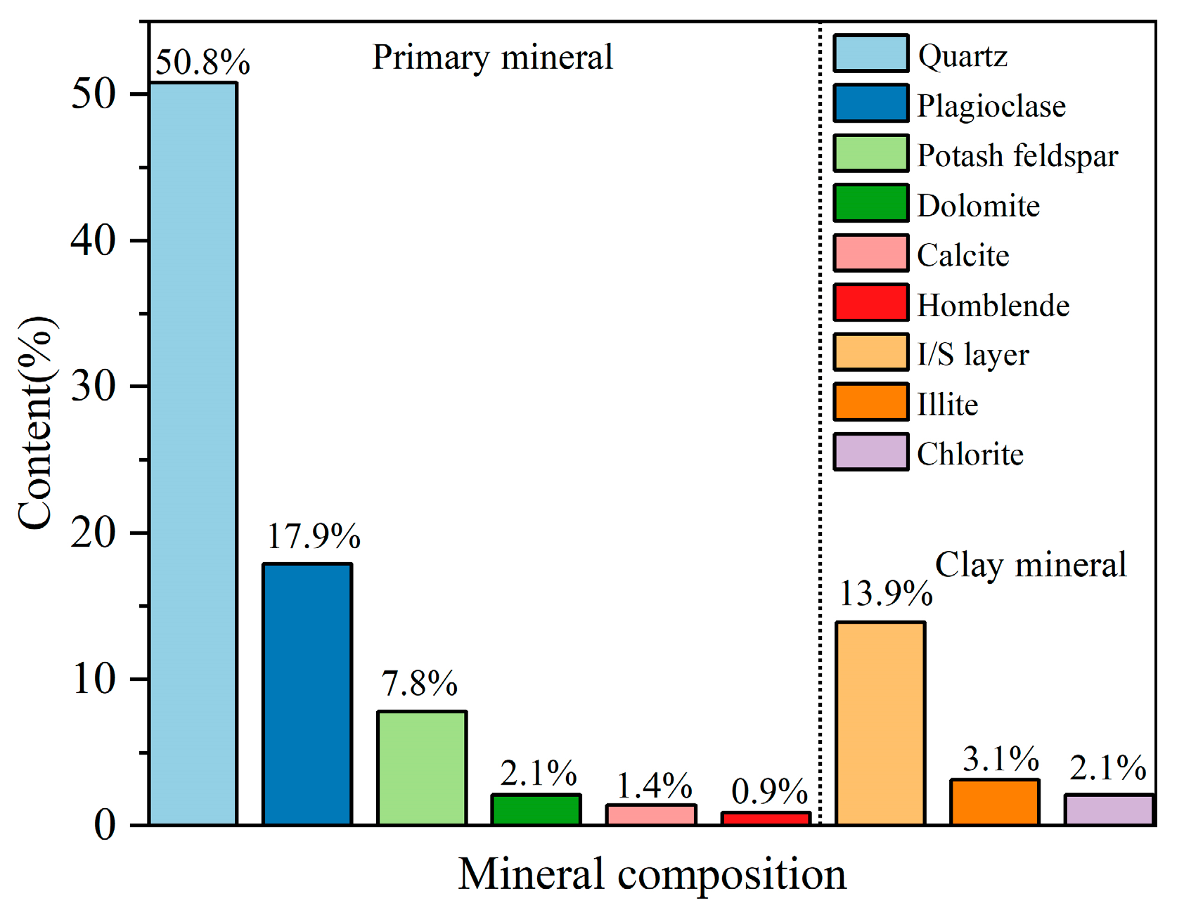
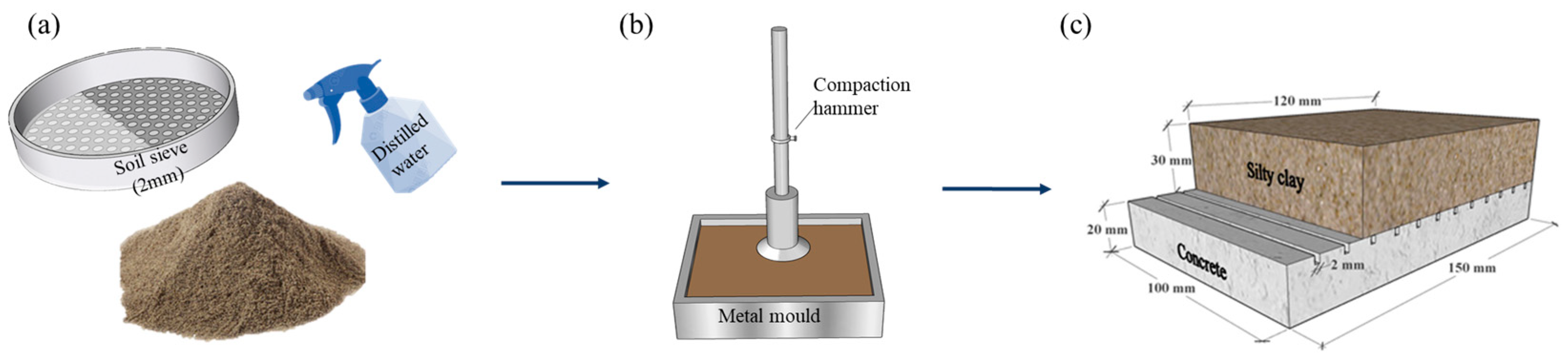
2.1. Sample Preparation

The environmental soil mass used to make the artificial interface was from Changchun City, Jilin Province, China (43°44′28″ N, 125°09′32″ E). Test samples were collected at a depth of 1 m below the surface. The sampling location and sampling site are shown in Figure 1a,b. According to the Unified Soil Classification System (USCS) [26], the soil was classified as lean clay, which has fine particles, strong water absorption after ramming, and good plasticity after wetting. It is also a type of loess-like soil.

Table 1. Basic properties of the soil.

Particle Diameter (%)			Optimum Water Content (%)	Maximum Dry Density (g/cm3)	Liquid Limit (%)	Plastic Limit (%)
2–0.075 mm	0.075–0.005 mm	<0.005 mm
1.4	66.06	32.54	20.7	1.64	34.39	19.04

summarizes the main engineering properties of the test soil samples. The maximum dry density represents the highest dry unit weight a soil sample can achieve at an optimum moisture content. The mineral composition of the soil was acquired through X-ray diffraction analysis (Figure 2).

The concrete strength grade was C30, and the dimensions of the concrete, measured from edge to edge, namely the length, width, and height of the concrete slab, were 150 mm, 100 mm, and 20 mm. The mix ratio of concrete is shown in

Table 2. Basic properties of the concrete (kg/m³).

Water	Cement	Sand	Gravel	Superplasticizer
180	360	705	1155	1.44

. The actual damage surface of soil pile foundation was selected as the roughness [27]. The roughness of concrete surface (joint roughness coefficient, JRC) was calculated using the modified sand filling method (Equation (1)) [17]. The JRC was 0.55, which was poured on the upper surface of concrete by a 3D printing template. The grooves were 2 mm wide and 3 mm deep, and each spacing was 10 mm. The concrete slab with grooves is shown in Figure 3.

$$JRC={\displaystyle \frac{d_{\max }}{\overline{d}}}\left[1+{\left({\displaystyle \frac{n_g}{n_{\mathrm{c}}+n_{\mathrm{g}}}}\right)}^3\right]{\displaystyle \frac{v_{\mathrm{s}}}{S}}$$

(1)

where $\overline{d}$ is the average depth of grooves on the surface of concrete blocks, d_max is the slip thickness of clay–concrete shear interface, d_max = (7~8) D₅₀; when $\overline{d}$ ≤ d_max, set d_max/$\overline{d}$ = 1, n_c is the number of grooves on the concrete surface, n_g is the number of smooth areas on the concrete surface, v_s is the volume of sand grouting, and S is the area of sand grouting.

First, the air-dried soil was passed through a 2 mm sieve and progressively humidified over a brief period using a sprayer filled with a calculated volume of distilled water until the desired water content was achieved. Second, all samples were cured at a standard temperature for 24 h to ensure uniform water distribution in the soil. Third, the soil samples were rammed into three layers with a 95% compaction degree in the upper shear box, and the excess soil was removed. The samples were wrapped in fresh-keeping film to prevent water evaporation. Finally, lean clay was placed on the upper layer, and the concrete slab was placed on the lower layer. The lean clay–concrete sample is shown in Figure 4.

2.2. Experimental Grouping and Design

2.2.1. Experimental Grouping

The experimental grouping under different influencing factors is shown in

Table 3. Experimental grouping.

Groups	Number	Initial Water Content/%	Normal Stress/kPa	Shear Displacement/mm	Number of Samples
G1	G1-JX	20.7	300	0, 3, 6, 9, 12	25
G2	G2-JX	20.7	400	0, 3, 6, 9, 12	25
G3	G3-JX	20.7	500	0, 3, 6, 9, 12	25

Notes: X in the numbering corresponds to shear displacement. For example, ‘G1-J12′ represents the group of tests conducted under a normal stress of 300 kPa with a shear displacement of 12 mm.

. In engineering practice, backfill compaction is typically performed based on the optimum moisture content as the standard for fill material. To better simulate real engineering conditions, the optimum moisture content was selected for this study. Also, existing studies have shown that the formation of a shear band requires a normal stress greater than 200 kPa [28]. Considering the practical engineering background, this study selected normal stresses of 300 kPa, 400 kPa, and 500 kPa under the optimum moisture content for the experiments. Additionally, five shear displacements (0, 3, 6, 9, and 12 mm) were considered. Each condition has five parallel samples, resulting in a total of 75 test groups. Among these, two samples were used to determine the dry density of the soil after direct shear tests, while the remaining three samples were used for moisture migration experiments.

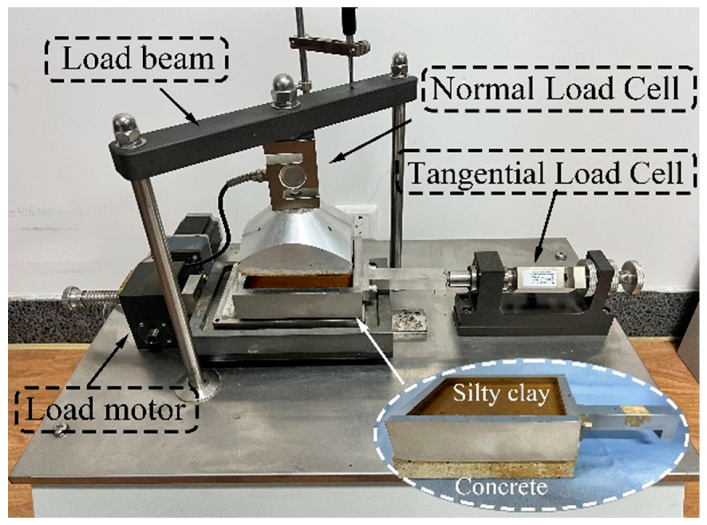
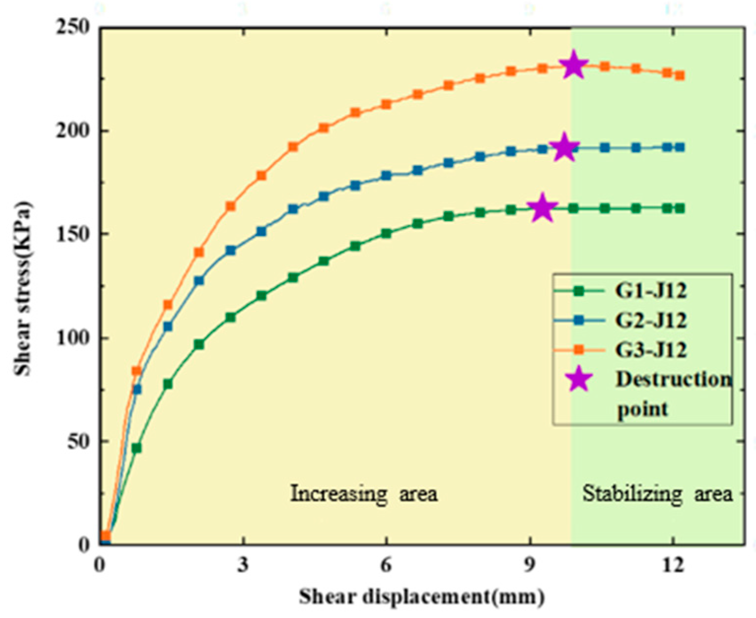
2.2.2. Direct Shear Test

In traditional direct shear instruments, the contact area between the upper and lower shear box progressively decreases during the shearing process, resulting in significant stress concentration. To address this issue, an improved direct shear apparatus was used to construct a shear band, as shown in Figure 5. Wang et al. [28] used PIV (Particle Image Velocimetry) technology to determine that the thickness of the shear band was about 10 mm when the roughness was 0.55. Therefore, the failure point was determined by the direct shear test. A shear band with a thickness of approximately 10 mm was constructed, and the dry density of soil inside and outside the shear band before and after the interface failure was measured. The influence of shear band on the dry density of soil within a certain range of the interface area between lean clay and the structure was studied, and the compaction of soil particles in the interface area under shear action was analyzed. The inner dimensions of the upper shear box in the direct shear apparatus were 120 × 100× 35 mm, and those of the lower shear box were 150 × 100 × 20 mm.

The lean clay was placed in the upper shear box, and the rough concrete plate was placed in the lower shear box. Using a computer-controlled system, the normal stress was gradually applied to the specimen until the target normal stress (300, 400, or 500 kPa) was reached. Once the target normal stress was applied, the vertical displacement of the specimen was continuously recorded using a displacement transducer to monitor the amount of compressibility. To prevent moisture loss, the soil specimen was wrapped with a damp cloth, maintaining the water content at its initial level. The compression was considered complete when the rate of vertical displacement became less than 0.005 mm/h [29]. Upon completion of the compression, the direct shear test was performed on the specimen under controlled conditions. After the direct shear test, the soil layer was divided inside and outside the shear band with a custom-made cutting ring (Φ 61.8 mm × 10 mm). Samples were obtained from each part. The water content of the samples was measured by the drying method, and the dry density was calculated.

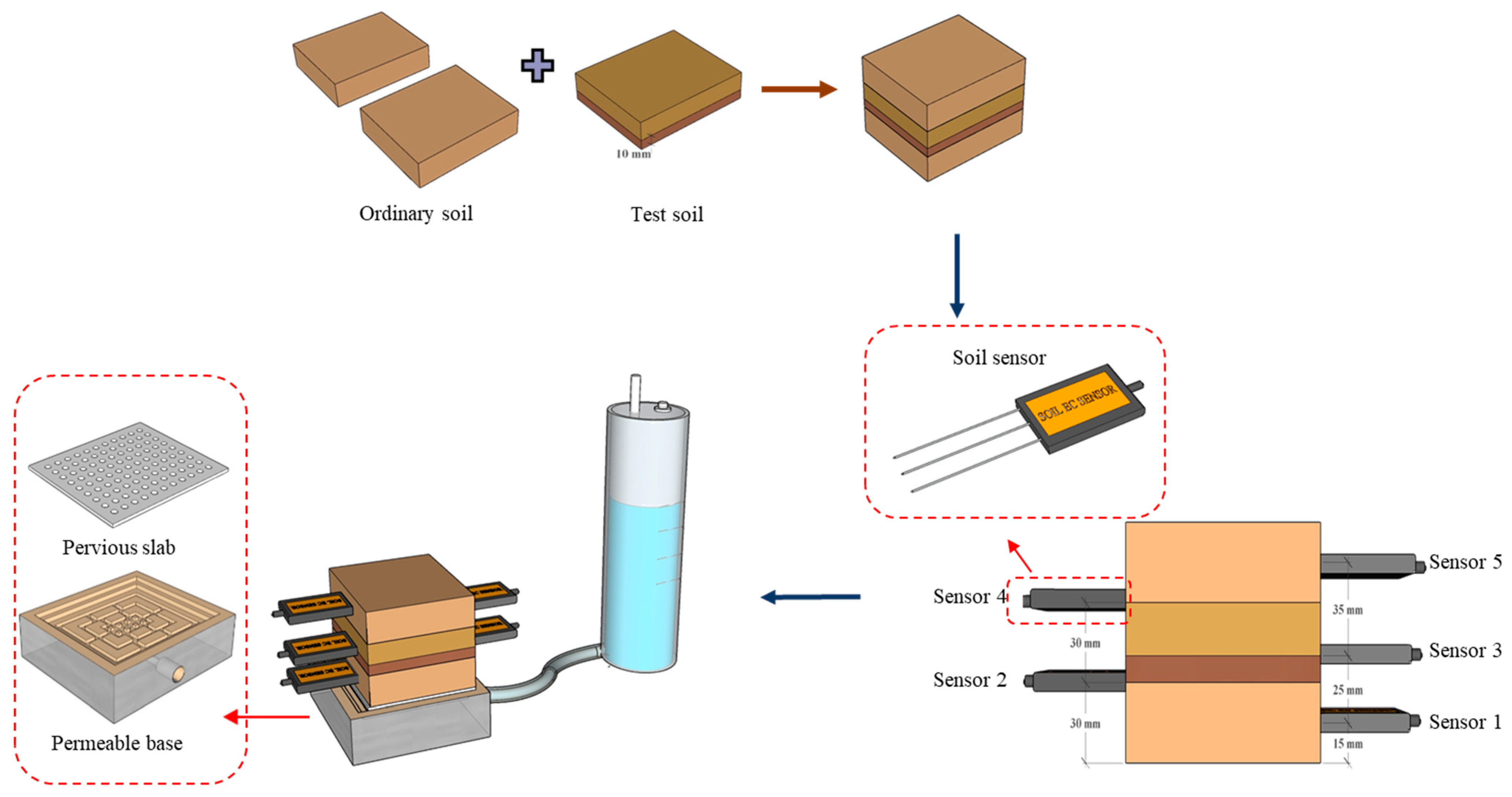
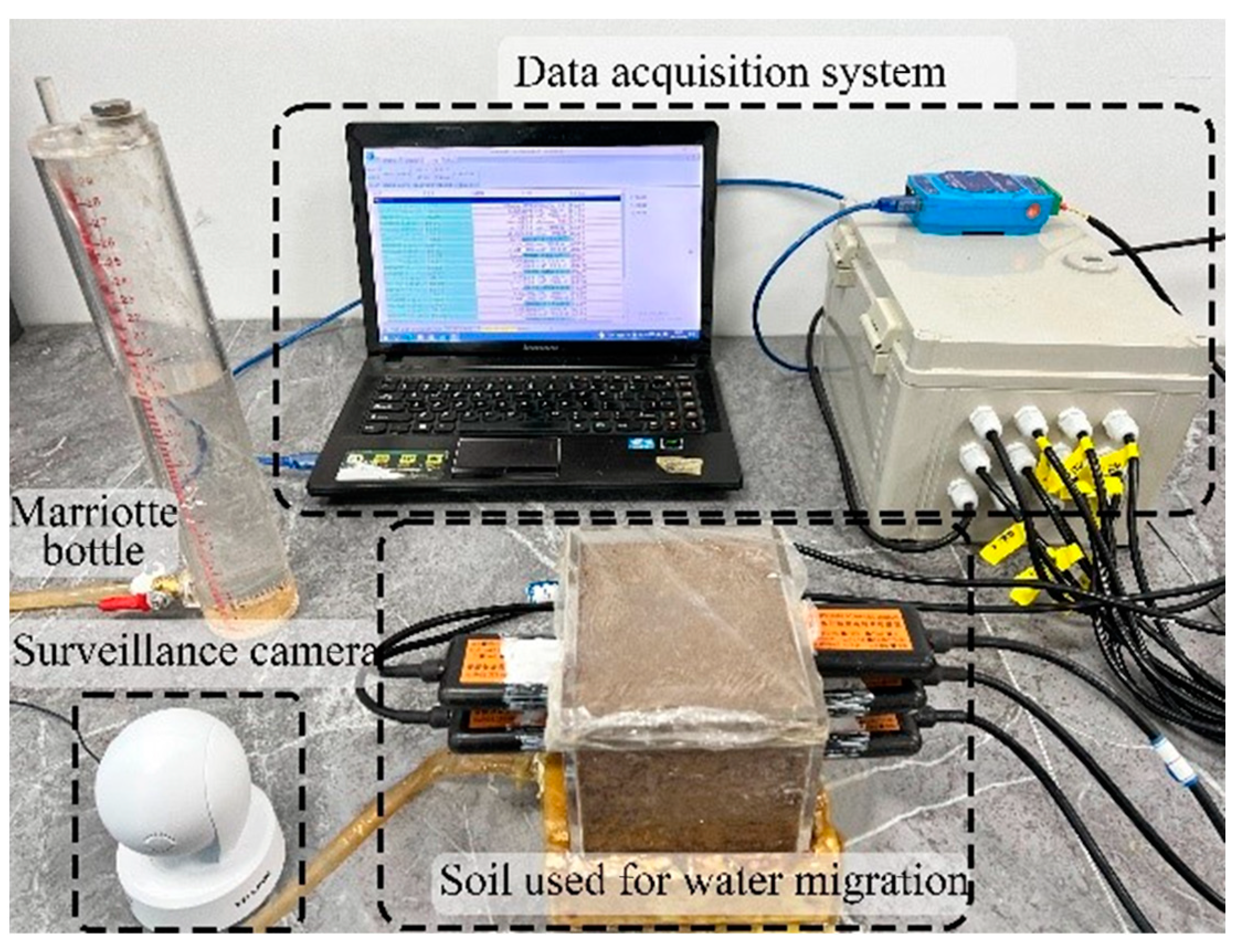
2.2.3. Soil Water Migration Test with the Shear Band

The influence of the shear band in the interface area between the lean clay and the structure on the water migration pattern in soil was explored. Two uncompressed ordinary soil layers under the same conditions as those for the test soil layer (initial water content and compactness) were prepared and placed above and below the test soil layer (test block after the direct shear test) to simulate the upward migration of water from the lower ordinary soil layer. The five sensors were, respectively, inserted at 15 mm, 30 mm (bottom of the shear band), 40 mm (top of the shear band), 60 mm (top of the test soil layer), and 75 mm (ordinary soil layer) from the bottom height. A Mariotte bottle was utilized to replenish water so that the bottom of the air inlet pipe was at the same level as the soil base. Also, a pervious slab was positioned atop the permeable base. The pervious slab was capable of preventing the dispersion of the soil bottom and enabling a more uniform flow of the solution into the soil. The water was sucked into the upper soil layer by the matrix suction of the soil (Figure 6). The test time was 24 h, and after the test, samples were obtained from the layers on the basis of the sensor positions for water content measurement using the drying method. The water migration device is shown in Figure 7.

3. Results and Discussion

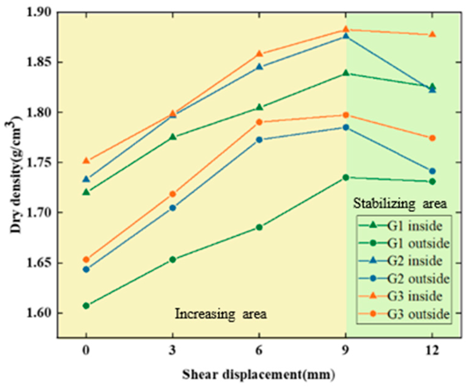
3.1. Analysis of the Dry Density of Soil in the Lean Clay–Concrete Shear Band

The dry density of soil inside and outside the shear band varied with shear displacement, as shown in

Table 4. Dry density test results (g/cm³).

Shear Displacement (mm)/Position	Group
	G1	G2	G3
0/Inside the shear band	1.7000	1.7331	1.7512
3/Inside the shear band	1.7752	1.7968	1.7985
6/Inside the shear band	1.8048	1.8452	1.8582
9/Inside the shear band	1.8390	1.8758	1.8827
12/Inside the shear band	1.8255	1.8519	1.8776
0/Outside the shear band	1.6071	1.6434	1.6533
3/Outside the shear band	1.6533	1.7049	1.7186
6/Outside the shear band	1.6854	1.7729	1.7904
9/Outside the shear band	1.7352	1.7852	1.7976
12/Outside the shear band	1.7311	1.7415	1.7745

and Figure 8. The presence of the shear band in the interface area between the lean clay and structure increased the dry density of soil, and the dry density of soil in the shear band was greater than that outside of it. The dry density of soil inside and outside the shear band demonstrated a positive correlation with normal stress. The results of the interface shear stress displacement curve of a lean clay–structural body were analyzed (Figure 9). The peak value was adopted as the shear strength when a peak value was observed on the shear stress–shear displacement curve. The results indicated that the dry density of the soil inside and outside the shear band gradually increased before the shear stress rose to the peak value, and when the interface area was damaged, the dry density of the soil inside and outside the shear band peaked. The reason for this is that before reaching the peak, the interface shear stress in the area between the lean clay and structure was supported by soil particle cohesion, soil–concrete interface interaction, and internal friction resistance. The soil particles were rearranged, and the internal structure was progressively compacted. When shear stress reached its peak, the soil particles were mostly compact; beyond the peak point, the interfacial shear zone was completely formed, shear stress was primarily supported by sliding friction between the soil and concrete interface, and the internal soil particles underwent minimal changes and even loosened slightly. At this point, the dry density of the soil mass inside and outside the shear band remained stable or showed a slightly decreasing trend.

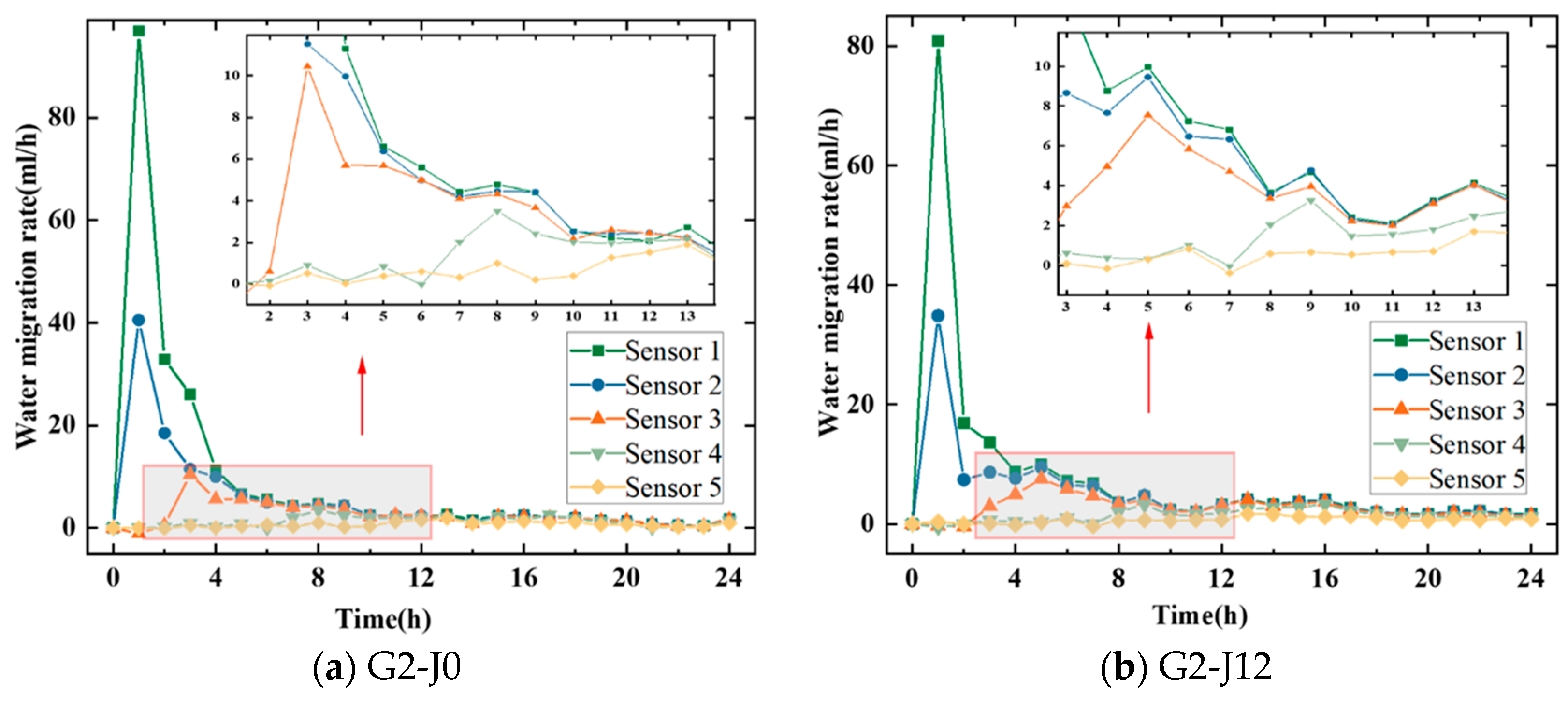
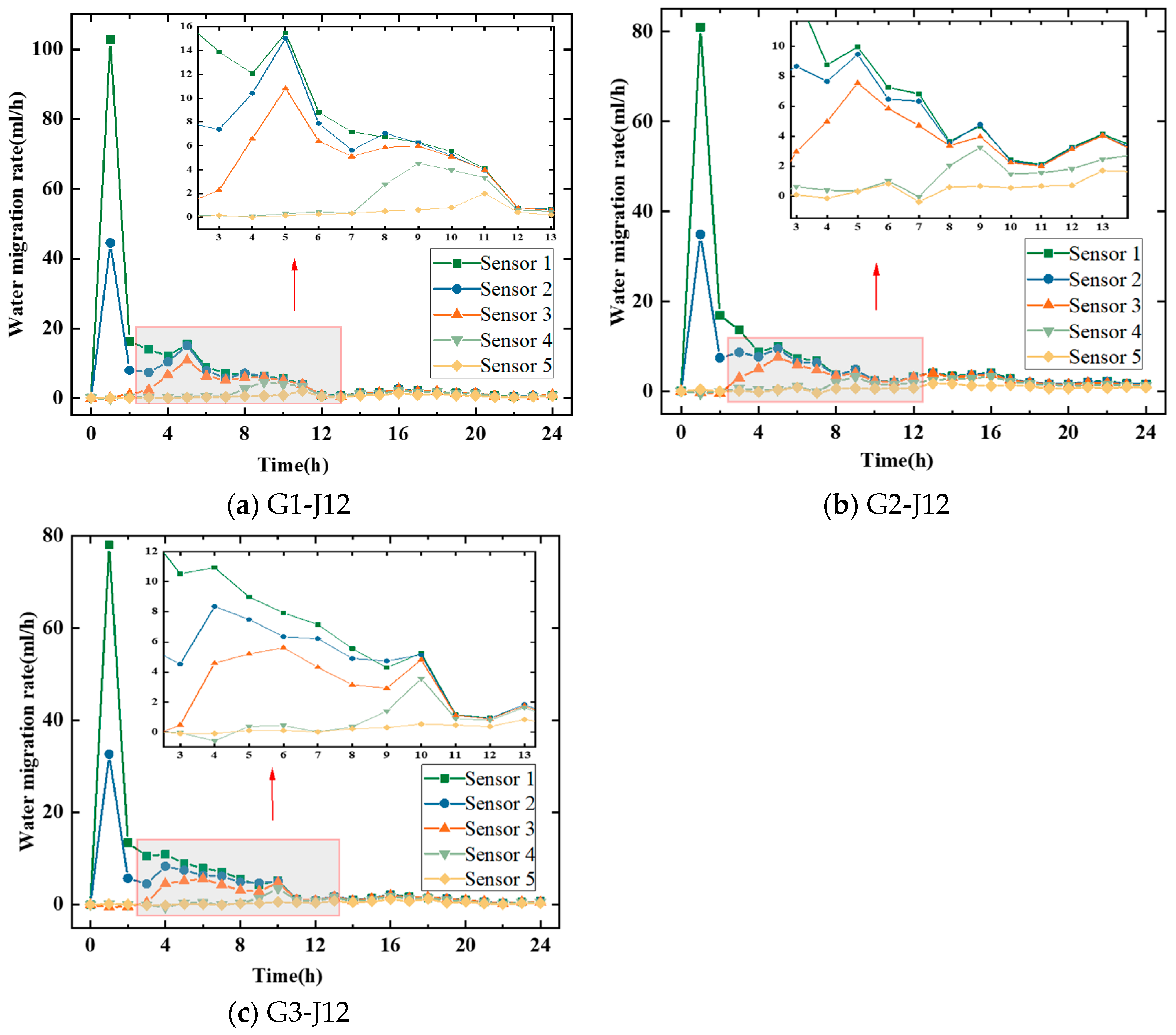
3.2. Changes in the Rate of Water Migration in Soil Under Different Influencing Factors

(1)

Shear Displacement

With the soil without a shear band in Group G2 (shear displacement of 0) and the soil with complete shear band formation (shear displacement of 12 mm) as examples, the water migration rate of the soil around the five sensors was plotted in Figure 10. Within the first hour from the beginning of the test, the water migration rate of the soil around Sensors 1 and 2 reached its peak, indicating that the water rapidly rose from the lower baseline soil layer during the initial stage of the test. Within two hours, the water rose to the bottom of the shear band of the test soil layer, and the water migration rate began to decrease due to the combined effects of the shear band and gravity potential. Within three hours, the water migration rate of the soil (shear band layer) around the two groups of Sensor 3 increased, although the water migration rate in Group G2-J0 was significantly higher than that in Group G2-J12. The water migration rate of Group G2-J0 peaked at 10.4360 mL/h at 3 h, while that of Group G2-J12 peaked at 7.5468 mL/h at 5 h, reflecting a reduction of 27.68%. Between 7 and 8 h, the water migration rate of the soil around Sensor 4 increased; however, the water migration was slow because the location was far from the water surface and was thus influenced by gravitational potential. The soil outside the shear band in the test soil layer of Group G2-J12 was also influenced by the soil inside the shear band. From 11 h to 13 h, the water migration rate of the soil around Sensor 5 increased slightly. A comparison of the time and rate changes in water migration around Sensors 4 and 5 revealed that water migration in Group G2-J12 began to increase and reach its peak value later than that in Group G2-J0, with a smaller peak value. In the G2-J12 group, due to the presence of the shear band, water was obstructed when reaching the bottom of the shear band. The gravitational potential effect weakened, the adsorption effect of soil particle surfaces on water increased, and the densely compacted shear band acted as a barrier to water migration. As a result, water required a longer time to penetrate the shear band, leading to a delayed and reduced peak water migration rate.

The slope of the fitted straight line for the rising segment (2–9 h) of the volumetric water content–time curve for Sensor 3 was calculated. It was found that as the shear displacement increased, and the slopes were 0.8394, 0.7382, 0.7263, 0.6527, and 0.7216, respectively. The shear displacement corresponding to the lowest rate of water content increase was 9 mm.

Table 5. Water migration rate (mL/h).

Group	Sensor 1	Sensor 2	Sensor 3	Sensor 4	Sensor 5
G2-J0	34.7652	17.3788	4.6260	2.3013	1.2683
G2-J3	28.6589	14.9105	4.5971	2.1800	1.1526
G2-J6	28.4000	14.4722	4.0581	2.0035	1.0656
G2-J9	26.1043	13.7580	3.7796	1.5002	0.7284
G2-J12	26.0233	13.6081	3.9069	1.9900	0.9814

Notes: sensors are numbered from bottom to top.

presents the average hourly water migration rates in the soil around each sensor during the rapid increase phase of volumetric water content in Group G2. It can be observed that, with the increase in shear displacement, the water migration rates of Sensors 3, 4, and 5 initially decreased and then slightly increased, with the lowest migration rate occurring at a shear displacement of 9 mm. This phenomenon is attributed to changes in the dry density of the soil layer under the influence of shear displacement. Within the shear band, the dry density first increased and then decreased. At a shear displacement of 9 mm, the dry density reached its maximum, resulting in the lowest porosity and the greatest resistance to water migration, thereby causing the slowest migration rate.

(2)

Normal stress

The soil water migration rate versus time curves for different normal stress values at a shear displacement of 12 mm are presented in Figure 11. As normal stress increased, the water migration rate in the soil decreased considerably. Specifically, in Groups G1-J12 and G2-J12, the water migration rate of the soil around Sensor 3 began to increase at 2 h and reached the peak values of 10.8224 and 7.5468 mL/h, respectively, at 5 h. The value for Group G2 decreased by 30.27% compared to that for Group G1. The water migration rate of the soil of Group G3-J12 around Sensor 3 began to increase at 3 h, but the water migration rate was low and exhibited a relatively smooth pattern. The water migration rate of the soil of Group G3-J12 reached its peak of 5.6192 mL/h at 6 h, indicating a decrease of 25.54% relative to the rate for Group G2-J12. These findings reveal that as normal stress increases, not only does the peak water migration rate decrease, but the time required to reach the peak also lengthens, demonstrating a slowing of the overall water migration process. Similar trends were observed in the water migration rate around Sensors 4 and 5. The higher normal stress resulted in lower water migration rates within the shear band, ultimately leading to slower water migration throughout the entire soil layer. As normal stress increases, the soil particles in the shear band are subjected to greater compaction, causing an increase in dry density and a corresponding decrease in porosity. The reduction in porosity diminishes the size and connectivity of the pore spaces that serve as pathways for water migration. Consequently, the movement of water through the shear band becomes increasingly restricted. This is particularly evident in Group G3, where the highest normal stress resulted in the smallest porosity and the lowest water migration rate.

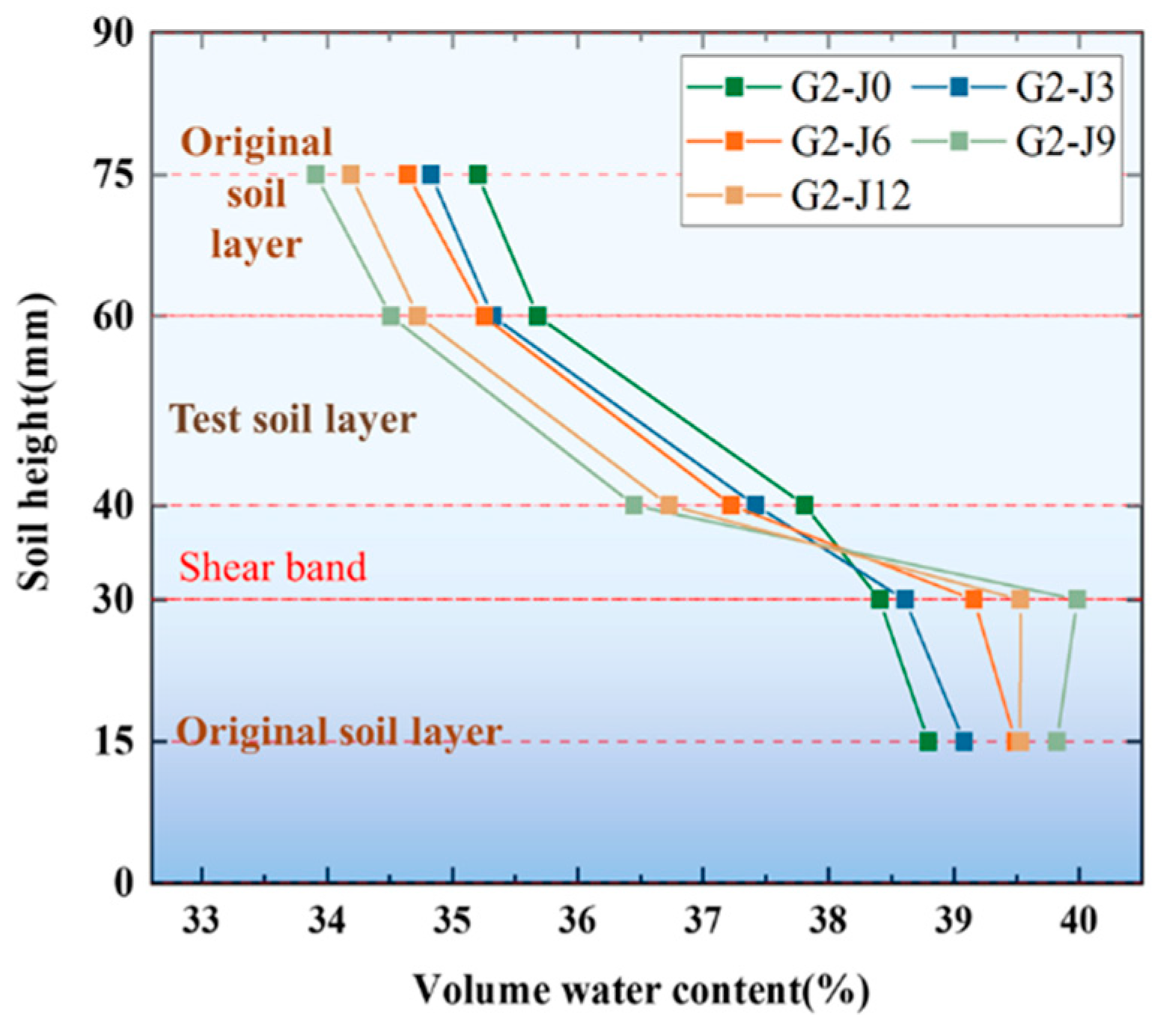
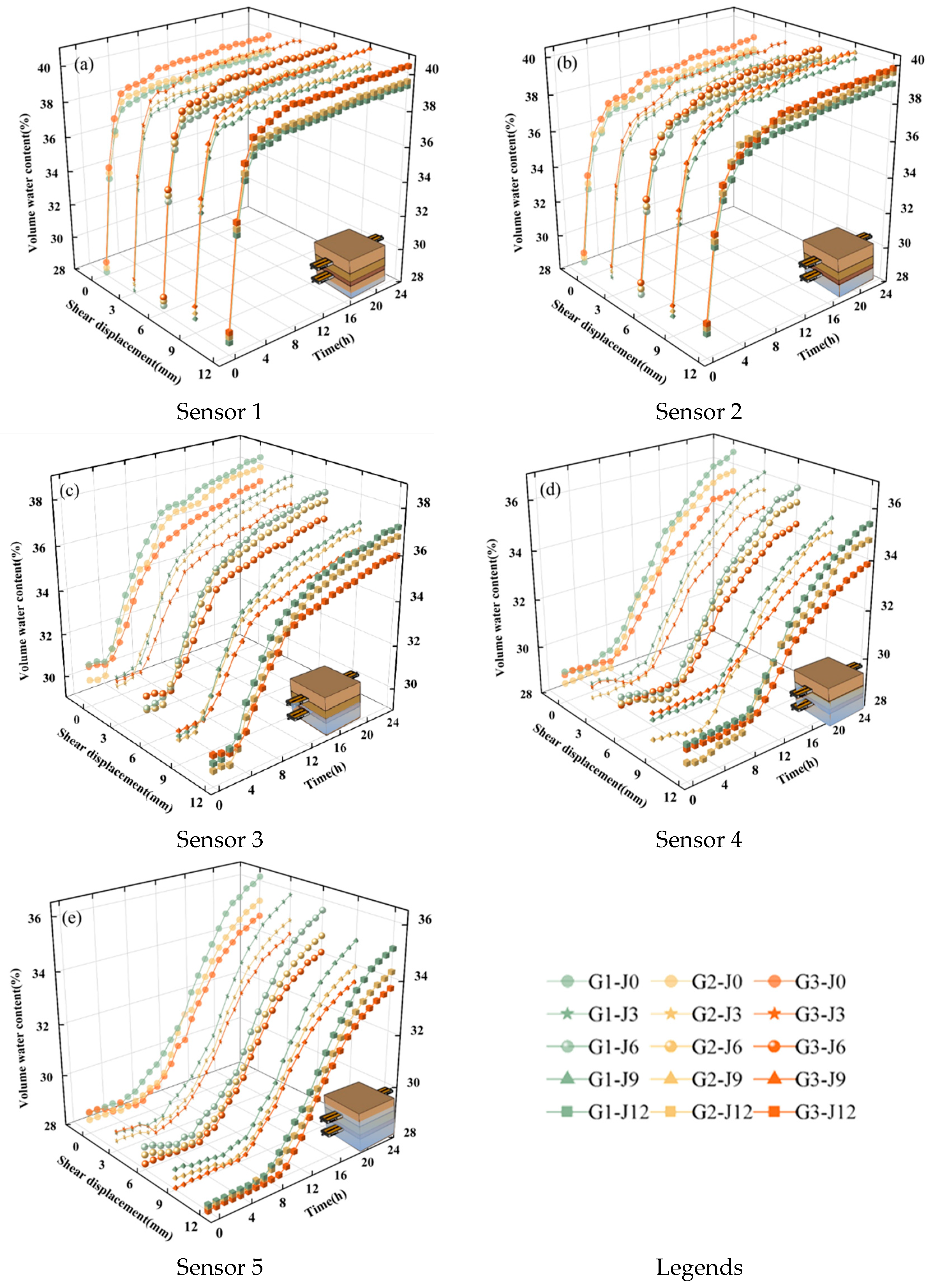
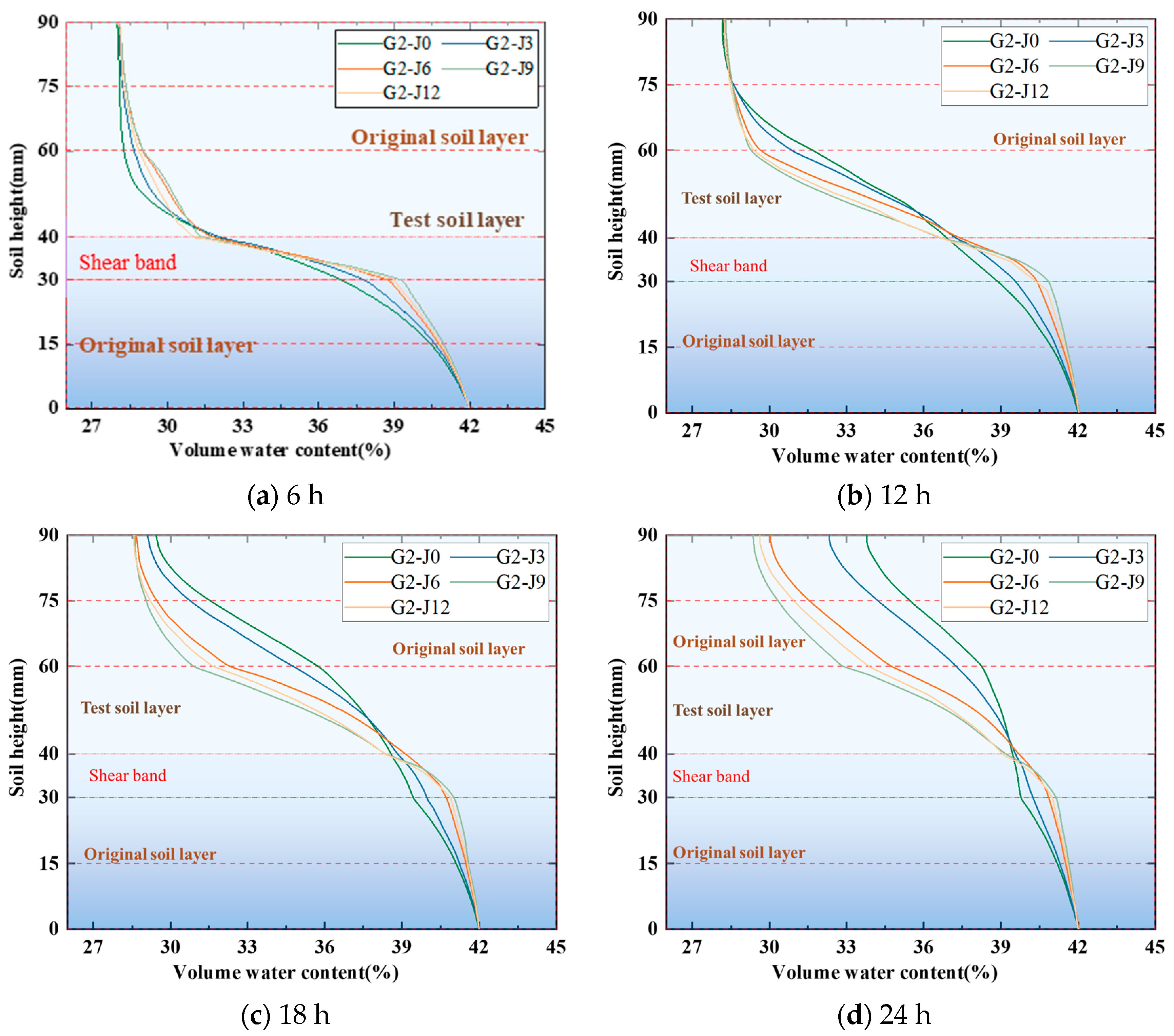
3.3. Changes in Soil Volume Water Content Under Different Influencing Factors

(1)

Shear Displacement

With Group G2 as an example, the data of representative Sensors 2, 3, and 4 and the volume water contents in relation to the change in shear displacement and time are presented in Figure 12. Figure 13 presents the distribution of soil volume water content at different heights under different shear displacements. At the beginning of the experiment, the volume water content of Sensor 2 rose rapidly, remained stable after 6–8 h, and increased then decreased as the shear displacement increased. The volume water contents of Sensors 3 and 4 began to rise after 3 h and 7–8 h, respectively, then decreased and increased with the increase in shear displacement. Sensor 2 was located at the lower part of the shear band. At this time, the volume water content of the soil without shear displacement was the smallest, and the volume water content of the soil with shear displacement of 9 mm was the largest. Sensors 3, 4, and 5 were positioned above the shear band. The volume water content of the unshear soil was the largest, and the volume water content of the soil with a shear displacement of 9 mm was the smallest. The volume water content was negatively correlated with the interfacial shear strength, suggesting that water was enriched in the shear band. This is a result of the densification and compaction of soil in the shear band under shear stress, which reduces the permeability of the soil and obstructs the upward migration of water. The inflection points of the curves were all at the shear displacement of 9 mm because the interface of the soil dry density in the shear band was broken when the shear displacement was 9 mm. Sensors 3, 4, and 5 were minimized because of the reduction in the over-water channel. At this critical displacement, the shear strength in the shear band was the highest, the soil dry density reached the peak, and the porosity of the soil was at its lowest, resulting in fewer pore spaces available for water to migrate. Sensors 1 and 2 were located below the shear band where the channel pores decreased, the closed pores increased, and water impermeability increased. At shear displacements of 9 and 12 mm, the volume water content of Sensor 2 was larger than that of Sensor 1, and water gathered at the top of the lower soil layer.

(2)

Normal stress

Figure 14 illustrates the change curve of the volume water contents of Sensors 1–5 with shear displacement and time. Under different shear displacements, the volume water content–time curves of Sensors 1 and 2 showed a trend of high volume water content at high normal stress after rising to the gentle section, but the change trends of Sensors 3, 4, and 5 were inverse. The higher the normal stress was, the lower the volume water content was because with the increase in normal stress, the interface shear strength increased, the soil in the test soil layer and shear band became dense, and impermeability was enhanced, which hindered the ascending channel of water and caused water to gather in the lower part of the shear band. In the upper part of the shear band, due to a decrease in soil porosity, the water migration rate slowed, and the volume of water content decreased.

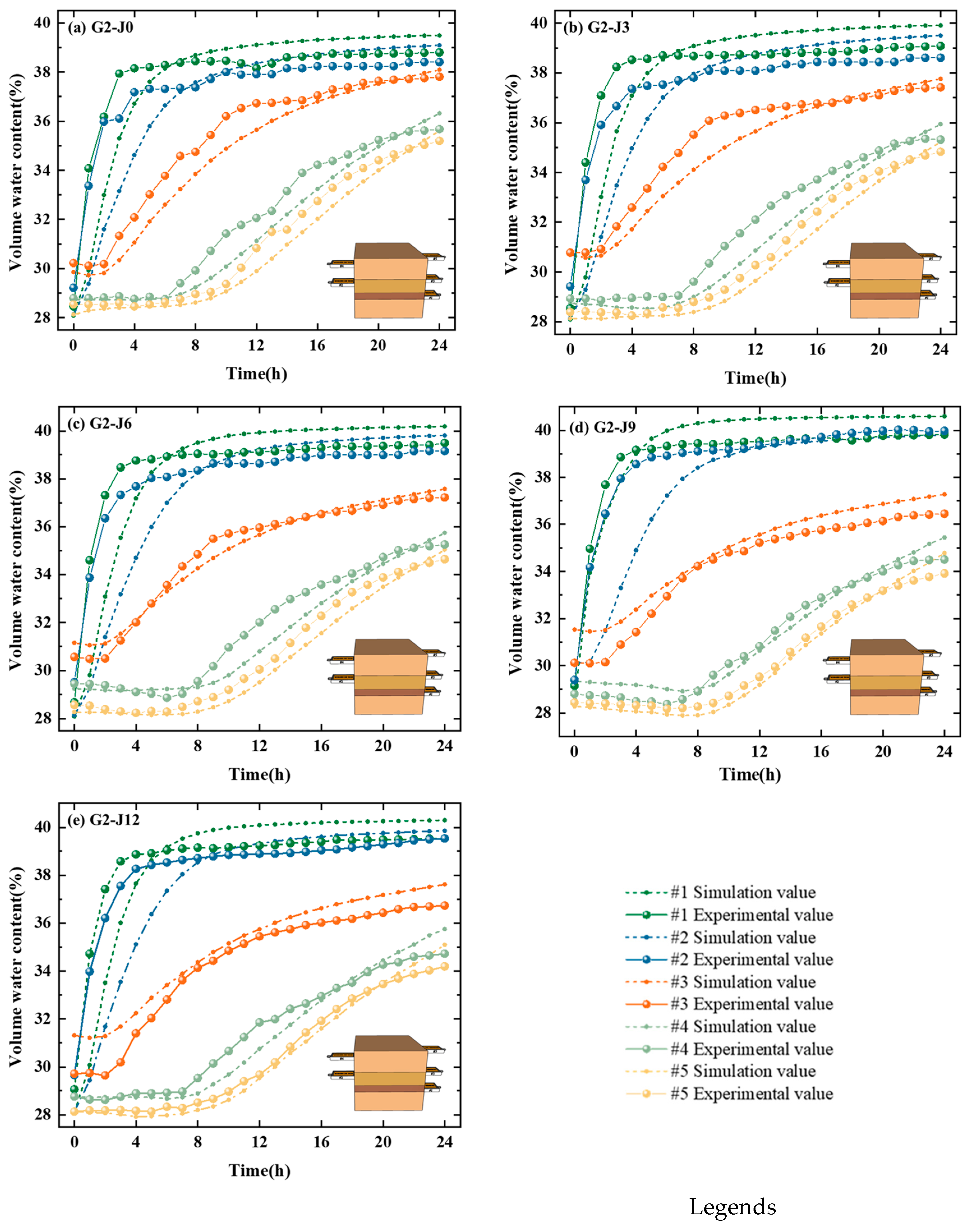
4. Numerical Simulation

4.1. Model Principle

In this test, the lateral migration of water in the soil was not considered, and the influence of gaseous water and temperature on water migration was excluded. The differential equation for water migration used Richards [30] for unsaturated porous media.

$${\displaystyle \frac{\partial \theta }{\partial t}}={\displaystyle \frac{\partial }{\partial x}}\left(K\left(\theta \right){\displaystyle \frac{\partial \phi }{\partial x}}\right)+{\displaystyle \frac{\partial }{\partial z}}\left(K\left(\theta \right){\displaystyle \frac{\partial \phi }{\partial z}}\right)$$

(2)

where $\theta$ is the volume water content of soil; $K\left(\theta \right)$ is the permeability coefficient of unsaturated porous media; and $\phi$ is the soil potential energy, matrix potential, and gravity potential, which were considered in this experiment. With the interface of the soil body in contact with the concrete as the origin, ${\phi }_g=z$. Therefore, $\phi ={\phi }_m+z$. Substitution into Equation (1) yields

$${\displaystyle \frac{\partial \theta }{\partial t}}={\displaystyle \frac{\partial }{\partial x}}\left(K\left(\theta \right){\displaystyle \frac{\partial \left({\phi }_m+z\right)}{\partial x}}\right)+{\displaystyle \frac{\partial }{\partial z}}\left(K\left(\theta \right){\displaystyle \frac{\partial \left({\phi }_m+z\right)}{\partial z}}\right)$$

(3)

The Hamiltonian operator was introduced, and the equation for water migration in the unsaturated soil in the numerical simulations was obtained as follows:

$${\displaystyle \frac{\partial \theta }{\partial t}}=\nabla \left[K\left(\theta \right)\nabla {\phi }_m\right]+\nabla \left[K\left(\theta \right)\right]$$

(4)

The Van Genuchten (1980) [31] model was used to determine matrix suction ${\phi }_m$ and permeability coefficient $k\left(\theta \right)$ of the unsaturated porous medium of the soil in Equation (5). The VG model is expressed as

$${\phi }_m={\displaystyle \frac{1}{a}}{\left({\displaystyle \frac{1}{{\left(S_{\mathrm{r}}\right)}^{\frac{1}{m}}}}-1\right)}^{{\displaystyle \frac{1}{n}}}$$

(5)

where $a,m,n$ are soil-related parameters and $m=1-1/n$ $S_r$ is the effective saturation of the soil, which has the following relationship with ${\theta }_s$ and ${\theta }_r$:

$$S_{\mathrm{r}}={\displaystyle \frac{\theta -{\theta }_{\mathrm{r}}}{{\theta }_{\mathrm{s}}-{\theta }_{\mathrm{r}}}}$$

(6)

where ${\theta }_s$ is the saturated water content of soil and ${\theta }_r$ is the residual water content of soil.

The permeability coefficient of unsaturated porous media is expressed as follows:

$$K\left(\theta \right)=k_{\mathrm{s}}{S}_{\mathrm{r}}^{0.5}{\left[1-{\left(1-S_{\mathrm{r}}^{{\displaystyle \frac{1}{m}}}\right)}^m\right]}^2$$

(7)

where $k_s$ is the permeability coefficient of saturated soil.

The parameters θ_s and θ_r were obtained from the curves generated by combining the RETC 6.02 software and the pressure plate apparatus, ensuring their accuracy. The parameters a, n, and m were derived using the empirical formulas established by Peng et al. [32] in the VG model for lean clay, which relates dry density to matric suction. The dry density of soil under different initial conditions was measured in this study to calculate the relevant parameters of soil quality, characterize the differences in soil under different initial conditions, and quantify the influence of shear action on soil water migration. The formulas are as follows:

$$\left\{\begin{array}{c}\alpha =5.7537{\rho }_d^{-12.802}+0.9492\\ \begin{array}{c}n=-3.8706{\rho }_d^2+12.305{\rho }_d-8.185\\ m=1-{\displaystyle \frac{1}{n}}\end{array}\end{array}\right.$$

(8)

4.2. Parameter Values

With Group G2 as an example,

Table 6. The values of relevant parameters of the differential equation.

Position		Inside/Outside Shear Band					Ordinary Soil
	Shear Displacement	0 mm	3 mm	6 mm	9 mm	12 mm
Parameters
a (^10−3 kPa−1)		5.043/9.951	3.177/6.221	2.260/3.769	1.830/3.450	2.157/4.474	6.404
m		0.400/0.368	0.300/0.352	0.255/0.317	0.217/0.309	0.247/0.336	0.354
n		1.515/1.583	1.429/1.543	1.342/1.465	1.277/1.447	1.328/1.505	1.547
${\theta }_s$ (%)		0.42
${\theta }_r$ (%)		0.045
ks (^10−10 m/s)		2.772/3.680	2.250/3.034	1.911/2.435	1.719/2.338	1.867/2.697	6.165

shows the values of the differential equation parameters.

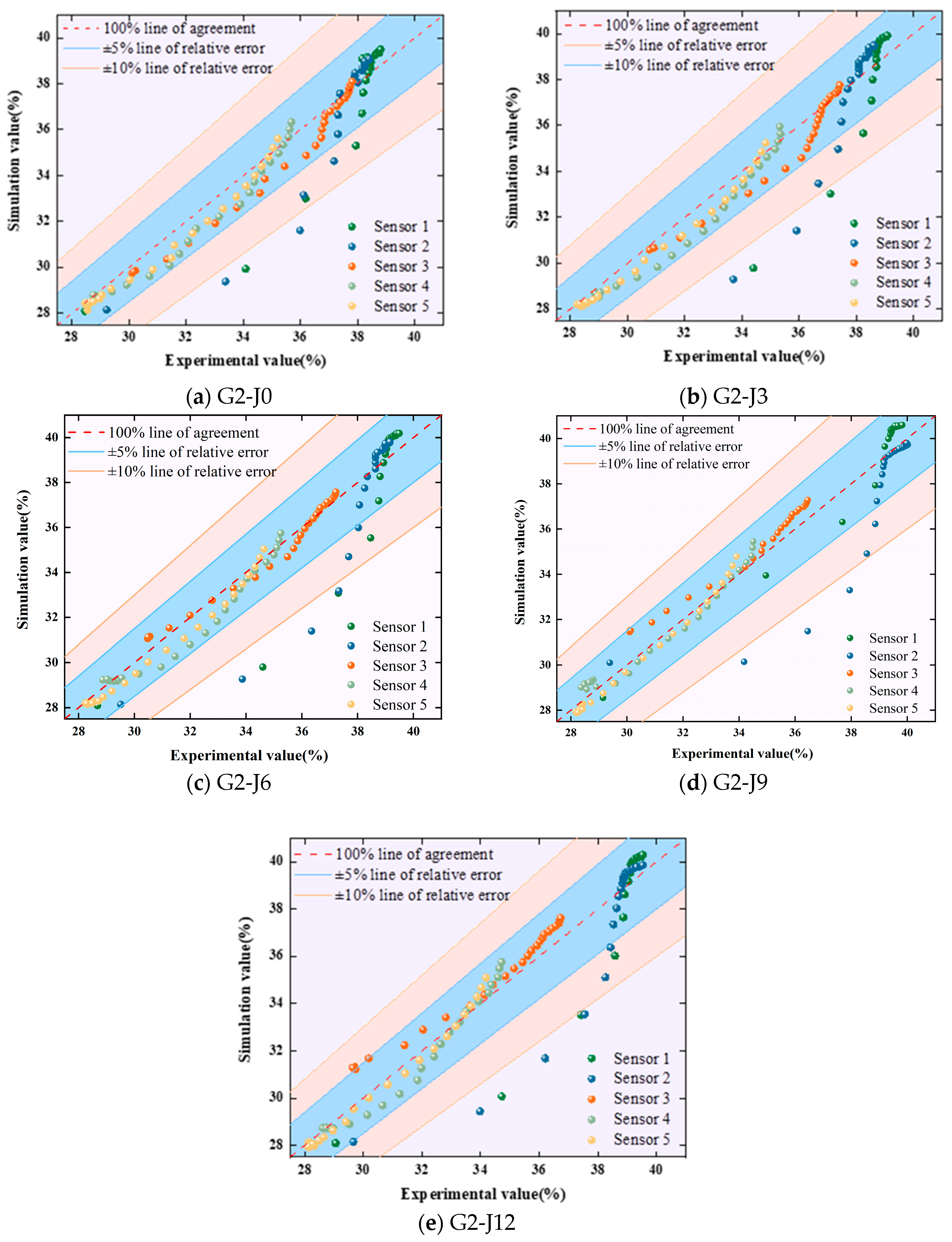
4.3. Model Verification and Prediction

Figure 15 and Figure 16 present the comparisons and relative error plots of the data points of the sensors in the numerical simulation and water migration test. The numerical calculation curves of Sensors 3, 4, and 5 showed good agreement with the test data points, and the relative error was less than 5%. An error was observed between the test and simulated values of Sensors 1 and 2. The relative error of some individual data exceeded 10%, and the maximum error was 13.86%, all of which occurred at the beginning of the test. This result was possibly due to the proximity of Sensors 1 and 2 to the horizontal plane and the high sensitivity of the sensors to water, which resulted in a rapid increase in the measured value at the early stage of the test. In general, the error in the numerical calculation results was smaller than that of the experimental data, indicating that the simulation results were reliable.

Given the limitations of this study, the change in the volume of water content in the soil was impossible to measure at any position and time during the test. Through numerical calculation and with 6, 12, 18, and 24 h as examples, Figure 17 shows the curve of the volume water content and height of the soil under five shear displacements in Group G2. The curve indicates that the soil volume water content exhibited a nonlinear relationship with changes in height, and the soil water content inside and outside the shear band gradually increased with time. The curves exhibited distinct turning points at the test soil layer, indicating that the different soil states in the shear band and test soil layer influenced water migration.

The above research results indicate that the presence of a shear band delays water migration in the soil, leading to moisture accumulation at the base of the shear band, specifically at the interface. This increase in water content at the interface is identified as a critical factor contributing to interface failure. These findings provide valuable insights for hydraulic engineering design in areas with similar soil characteristics, such as improving the soil in the interface band to facilitate better water migration. However, it is important to note that the experimental setup has limitations. For example, the specimen dimensions used in the laboratory are significantly smaller than those in real-world applications. Future studies should consider the effects of scale, as well as the influence of cyclic loading, freeze–thaw cycles, the range of shear displacements and normal stresses, and other multifactorial conditions, to enhance the applicability of the findings to practical engineering scenarios.

5. Conclusions

In this study, direct shear tests, water migration tests, and numerical simulations were conducted on loess-like soil in the Changchun area. The shear band was formed through a direct shear test on the lean clay–structure interface, and the water migration behavior in the soil within the interface area containing the shear band was studied. The main conclusions are as follows:

(1)

The water migration rate of the soil containing the shear band in the interface area decreased. A substantial amount of moisture accumulated within the shear band, and the water content was positively correlated with the shear strength of the interface.

(2)

The shear displacement and normal stress significantly affect moisture migration within the interface region. With the increase in shear displacement, the volume water content of the soil in the shear band decreased initially and then increased, and the inflection point corresponded to the displacement at which the interface failed. The volume water content of the soil in the shear band exhibited a negative correlation with normal stress.

(3)

A numerical model of water migration within the lean clay–structure interface region with a shear band was established. The model effectively simulates the process of water migration in the lean clay–structure interface region.

References

1. Singh, M.P.; Sen, S.; Pathak, H.; Dogra, A.B. Early age cracking relevant to mass concrete dam structures during the construction schedule. Constr. Build. Mater. 2024, 411, 134739. [Google Scholar] [CrossRef]
2. Hashemi, A.; Sutman, M.; Abuel-Naga, H. Thermomechanical response of kaolin clay–concrete interface in the context of energy geostructures. Can. Geotech. J. 2022, 60, 380–396. [Google Scholar] [CrossRef]
3. Brown, E. Reducing risks in the investigation, design and construction of large concrete dams. J. Rock Mech. Geotech. Eng. 2017, 9, 197–209. [Google Scholar] [CrossRef]
4. Lv, Y.; Shen, Y.; An, L.; Wei, X.; Chen, X.; He, R.; Shi, B.; Zhou, Z. A novel cement-based interface functional material for application onto shotcrete-rock interface of tunnel in cold regions. Constr. Build. Mater. 2024, 438, 136923. [Google Scholar] [CrossRef]
5. Liu, S.; Zhang, B.; Wang, H.; Cheng, J.; Cai, C.; Wang, X.; Lv, C. Large-scale field test on the shear behavior of concrete pipe-silty soil interfaces in pipe jacking: A case study. Construct. Build. Mater. 2024, 419, 135470. [Google Scholar] [CrossRef]
6. Zhang, D.; Lu, T. Establishment and application of an interface model between soil and structure. Chin. J. Geotech. Eng. 1998, 20, 65–69. [Google Scholar]
7. Qin, Y.; Shang, C.; Li, X.; Lai, J.; Shi, X.; Liu, T. Failure mechanism and countermeasures of rainfall-induced collapsed shallow loess tunnels under bad terrain: A case study. Fail. Anal. 2023, 152, 107477. [Google Scholar] [CrossRef]
8. Zhou, S.; Tian, Z.; Di, H.; Guo, P.; Fu, L. Investigation of a loess-mudstone landslide and the induced structural damage in a high-speed railway tunnel. Bull. Geol. Environ. 2020, 79, 2201–2212. [Google Scholar] [CrossRef]
9. Shen, Y.; Tang, T.; Wang, D.; Chen, M.; Liu, Y.; Wang, Y. Nonzero angle between the directions of matric suction and gravity during horizontal freezing. Acta Geotech. 2024, 19, 821–831. [Google Scholar] [CrossRef]
10. Li, H.; Yan, C.; Shi, Y.; Sun, W.; Bao, H.; Li, C. A statistical damage model for the soil-structure interface considering interface roughness and soil shear area. Constr. Build. Mater. 2024, 431, 136606. [Google Scholar] [CrossRef]
11. Campos, A.; Lopez, C.M.; Blanco, A.; Aguado, A. Effects of an internal sulfate attack and an alkali-aggregate reaction in a concrete dam. Constr. Build. Mater. 2018, 166, 668–683. [Google Scholar] [CrossRef]
12. Goodman, R.E.; Taylor, R.L.; Brekke, T. A model for the mechanics of jointed rock. J. Soil. Mech. Found. Div. 1968, 94, 637–659. [Google Scholar] [CrossRef]
13. Uesugi, M.; Kishida, H.; Tsubakihara, Y. Behavior of sand particles in sand-steel friction. Soils Found. 1988, 28, 107–118. [Google Scholar] [CrossRef]
14. Uesugi, M.; Kishida, H.; Uchikawa, Y. Friction between dry sand and concrete under monotonic and repeated loading. Soils Found. 1990, 30, 115–128. [Google Scholar] [CrossRef]
15. Zhang, G.; Liang, D.; Zhang, J. Image analysis measurement of soil particle movement during a soil–structure interface test. Comput. Geotech. 2006, 33, 248–259. [Google Scholar] [CrossRef]
16. Wang, J.; Gutierrez, M.S.; Dove, J.E. Numerical studies of shear banding in interface shear tests using a new strain calculation method. Int. J. Numer. Anal. Met. 2007, 31, 1349–1366. [Google Scholar] [CrossRef]
17. Chen, X.; Zhang, J.; Xiao, Y.; Li, J. Effect of roughness on shear behavior of red clay– concrete interface in large-scale direct shear tests. Can. Geotech. J. 2015, 52, 1122–1135. [Google Scholar] [CrossRef]
18. Pan, J.; Wang, B.; Wang, Q.; Ling, X.; Fang, R.; Liu, J.; Wang, Z. An adhesion-ploughing friction model of the interface between concrete and silty clay. Constr. Build. Mater. 2023, 376, 131039. [Google Scholar] [CrossRef]
19. Wang, G.; Wei, X.; Zou, T. A hollow cylinder radial-seepage apparatus for evaluating permeability of sheared compacted clay. Geotech. Test. J. 2018, 42, 1133–1149. [Google Scholar] [CrossRef]
20. Alnmr, A.; Ray, R. Numerical simulation of replacement method to improve unsaturated expansive soil. Pollack Period. 2023, 18, 41–47. [Google Scholar] [CrossRef]
21. Alnmr, A.; Alzawi, M.O.; Ray, R.; Abdullah, S.; Ibraheem, J. Experimental Investigation of the Soil-Water Characteristic Curves (SWCC) of Expansive Soil: Effects of Sand Content, Initial Saturation, and Initial Dry Unit Weight. Water 2024, 16, 627. [Google Scholar] [CrossRef]
22. Pham, T.A.; Sutman, M.; Medero, G.M. Density-dependent model of soil–water characteristic curves and application in predicting unsaturated soil–structure bearing resistance. Int. J. Geomech. 2023, 23, 04023017. [Google Scholar] [CrossRef]
23. Lei, H.; Wu, Y.; Yu, Y.; Zhang, B.; Lv, H. Influence of Shear on Permeability of Clayey Soil. Int. J. Geomech. 2016, 16, 04016010. [Google Scholar] [CrossRef]
24. Liu, Q.; Yu, Y.; Zhang, B.; Wang, X.; Lv, H.; Zhan, Z. A new apparatus for shear-seepage testing at the clayey soil-structure interface. Geotech. Test. J. 2022, 45, 281–299. [Google Scholar] [CrossRef]
25. Zeng, Z.; Tang, C.; Cheng, Q.; An, N.; Yang, Z.; Gong, X.; Chen, X.Y. Field and numerical investigation of soil hydro-thermal response to the climatic conditions in southern China considering soil heterogeneity. Eng. Geol. 2024, 329, 107401. [Google Scholar] [CrossRef]
26. ASTMD2487-17; Standard Practice for Classification of Soils for Engineering Purposes (Unified Soil Classification System). ASTM International: West Conshohocken, PA, USA, 2017.
27. Fang, R.; Wang, B.; Pan, J.; Liu, J.; Wang, Z.; Wang, Q.; Ling, X. Effect of concrete surface roughness on shear strength of frozen soil–concrete interface based on 3D printing technology. Constr. Build. Mater. 2023, 366, 130158. [Google Scholar] [CrossRef]
28. Pan, J.; Wang, B.; Wang, Q.; Ling, X.; Fang, R.; Liu, J.; Wang, Z. Thickness of the shear band of silty clay–concrete interface based on the particle image velocimetry technique. Constr. Build. Mater. 2023, 388, 131712. [Google Scholar] [CrossRef]
29. GB/T50123-2019; Standard for Geotechnical Test Methods. China Planning Press: Beijing, China, 2019.
30. Richards, L.A. Capillary conduction of liquids through porous mediums. J. Appl. Phys. 1931, 1, 318–333. [Google Scholar] [CrossRef]
31. Van Genuchten, M. A Closed-Form Equation for Predict in the Hydraulic Conductivity of Unsaturated Soils. Soil Sci. Soc. Am. J. 1980, 44, 892–898. [Google Scholar] [CrossRef]
32. Zhuang, X.; Peng, W. A simplified method for determining the model parameters of soil-water characteristic curve under different dry densities. J. Chang. River Sci. Res. Inst. 2019, 36, 64–67. [Google Scholar]
Figure 1. Sampling site profile: (a) Sampling location; (b) Sampling site.
Water 17 00350 g001
Figure 2. Mineral composition of the soil.
Water 17 00350 g002
Figure 3. Concrete slab process with grooves.
Water 17 00350 g003
Figure 4. Production process of the lean clay–concrete sample: (a) Soil sample preparation; (b) Soil sample compaction; (c) Lean clay-concrete sample.
Water 17 00350 g004
Figure 5. Direct shear device.
Water 17 00350 g005
Figure 6. Preparation procedure for water migration.
Water 17 00350 g006
Figure 7. Water migration device.
Water 17 00350 g007
Figure 8. Change in the dry density of soil inside and outside the shear band with shear displacement.
Water 17 00350 g008
Figure 9. Shear stress–shear displacement curve of the interface under normal stress.
Water 17 00350 g009
Figure 10. Soil water migration rates under different shear displacements.
Water 17 00350 g010
Figure 11. Water migration rate of soil under different normal stress values.
Water 17 00350 g011
Figure 12. Change in the soil volume water content of each sensor under different shear displacements.
Water 17 00350 g012
Figure 13. Volume water content of soil at different heights under different shear displacements.
Water 17 00350 g013
Figure 14. Change in the soil volume water content of each sensor under different normal stress values.
Water 17 00350 g014
Figure 15. Comparison of the experimental and simulation values of each group of sensors under different shear displacements.
Water 17 00350 g015
Figure 16. Relative error between the experimental and simulation values under different shear displacements.
Water 17 00350 g016
Figure 17. Volume water content of the soil at different heights and times.
Water 17 00350 g017