Cross-Sectional Variability of Suspended Sediment Concentration in the Rhine River

Abstract

Suspended sediment transport in large rivers is characterized by complex cross-sectional patterns. This study investigates the cross-sectional distribution of the suspended sediment concentration (SSC), based on 15 measurement campaigns at six stations along a 67 km reach of the middle Rhine in Germany. Utilizing a multi-method approach, we conducted turbidity and acoustic backscatter measurements, in situ particle size data, recorded water quality parameters such as electrical conductivity, and took 495 pump-based water samples over a period of 2.5 years. Statistical analysis of this comprehensive dataset shows that lateral differences have greater importance for the cross-sectional SSC distribution than vertical differences, suggesting that incomplete river mixing is of greater importance than vertical stratification for uncertainties in load calculations. We demonstrate that surface measurements are consistently representative for the whole water column and that applying the traditional Rouse equation for vertical extrapolation from surface measurements leads to large errors. We conclude that efficient monitoring programs should prioritize covering the lateral SSC distribution for more accurate load calculations and offer practical recommendations for improved SSC monitoring in similar conditions.

1. Introduction

Suspended sediments represent a major part of sediment loads in almost all lowland rivers of the world, as well as in the German federal waterways [1,2]. They play an essential role in the transport of nutrients, shaping of river channels and formation of ecological habitats, and are essential within the contexts of pollutant transport, ecological degradation and floods. Therefore, a comprehensive understanding of suspended sediments within rivers is inevitable for sediment and river management, both quantitatively and qualitatively [3,4].

Despite decades of research in this area, the spatial and temporal factors and processes, as well as the underlying interactions of suspended sediment transport in rivers, are insufficiently understood [3]. Since suspended sediments in rivers are mostly supply- instead of transport-limited [5], models fail to predict suspended sediment transport and comprehensive in situ monitoring; considering the cross-sectional and temporal variability of the suspended sediment concentration (SSC) is necessary.

The vertical variability of the SSC within river cross-sections is well-described in the literature and can be theoretically approximated, based on the physical properties of the observed suspended sediments—most importantly, particle size and density—from which the theoretical settling velocity of a particle can be calculated [6,7]. The settling of the particles is counterbalanced by turbulent mixing, which is strongly related to the shear velocity of the flowing water. Therefore, by knowing the physical properties of the stream flow and the suspended sediments, theoretical assumptions can be used to calculate the vertical distribution of sediments within the stream. Traditionally, this is performed using the Rouse equation, which describes SSC as a function of height above the channel bed:

$${\displaystyle \frac{C\left(z_b\right)}{C_a}}={\left({\displaystyle \frac{h-z_b}{z_b}}{\displaystyle \frac{a}{h-a}}\right)}^{Ro}={z_a}^{Ro}$$

(1)

where $C\left(z_b\right)$ is the SSC at height $z_b$ above the channel bed, $C_a$ is the SSC at the reference height $a$, $h$ is the water depth, and $Ro$ is the Rouse number. $z_a$ represents the relative depth, ranging from 1 at $a$ to 0 at the water surface.

The Rouse number is a function of the settling velocity, $w$, of the suspended matter and of the shear velocity of the flow, $u_{*}$, multiplied with the von Karman constant, $\kappa$:

$$Ro={\displaystyle \frac{w}{\kappa u_{*}}}$$

(2)

It is a measure for the gradient of the SSC with depth and is typically used to differentiate the bed load ($Ro>3$), suspended bed material load ($3>Ro>0.06$) and wash load ($Ro<0.06$) [8,9,10].

Since the settling velocity, w, is a function of particle size and density, it can vary substantially for primary particles in comparison to aggregated/flocculated particles, which are characterized by a larger size but substantially lower densities [11,12].

In contrast to vertical gradients, which have been investigated for various river systems, lateral variations in SSC within channel cross-sections have received far less attention. Therefore, there is no theoretical framework concerning the lateral distribution of suspended sediments in rivers, and a general shortage of studies taking lateral differences in SSC into account [7,13,14]. The lateral distribution of suspended sediment might depend on channel geometry, lateral distribution of shear stresses and curvature of the stream and river depth, as well as on lateral mixing processes and the influence of tributaries [13,15,16,17]. Albeit that lateral differences in SSC might be rather site-specific and hard to put in an applicable theoretical framework, neglecting their influence on load calculations and sediment budgeting leads to large errors.

Monitoring suspended sediments in rivers is a tedious task. Traditionally, SSC is measured by in situ point- or depth-integrating samples. Thereby, a mixture of sediment and water is collected via a physical sampler and analyzed in the laboratory for the gravimetric determination of SSC [18,19]. High-frequency (e.g., 15 min to daily) monitoring of the suspended sediment is mostly limited to point sampling. For example, suspended sediment monitoring along the German waterways, which started in the 1960s, has been conducted via work-daily 5 L grab samples taken at the main current, at approx. 65 monitoring sites [5]. This point sampling approach, however, has several drawbacks. Measuring SSC manually, daily and in situ is difficult, labor intensive, potentially hazardous, slow, expensive and requires practice [18]. There are many known reasons for errors using manual SSC measurement, including biased sampling based on the sampling location and uncertainties of laboratory analysis. Also, SSC samples are hardly taken at short sampling intervals that cover the high temporal variability of the suspended sediment transport [16]. These reasons support the usage of surrogate technologies for the measurement of SSC. Although they also suffer from limitations, due to measurement location and sample-based calibration, their continuous deployment improves the overall quality of monitoring and gives important insights into the temporal variability of SSC and averaging the gathered data reduces uncertainties stemming from micro-fluctuations in suspended particulate matter (SPM). The most prominent surrogates are optical turbidity—e.g., used in the German single-point surface measurements monitoring system—and acoustic backscatter measurements to derive the SSC within a waterbody [18,19,20]. The sample-based calibration may change over time, prompting the need for continuous sampling, which should be efficient and representative.

This study analyses a 67 km stretch of the free-flowing middle Rhine in Germany. The measurement concept is designed to answer the following research questions:

• Which measuring device or combination of devices is best suited to detect the spatial variability of suspended sediment concentrations and characteristics of suspended matter within the cross-sections of the Rhine River?
• Can vertical gradients of the SSC in the Rhine River be described using the Rouse equation and can the Rouse number be sufficiently predicted using the measured parameters?
• Which factors control lateral SSC gradients and how do lateral gradients relate to vertical gradients?
• What are the implications for monitoring the suspended sediment in large river systems?

2. Study Area

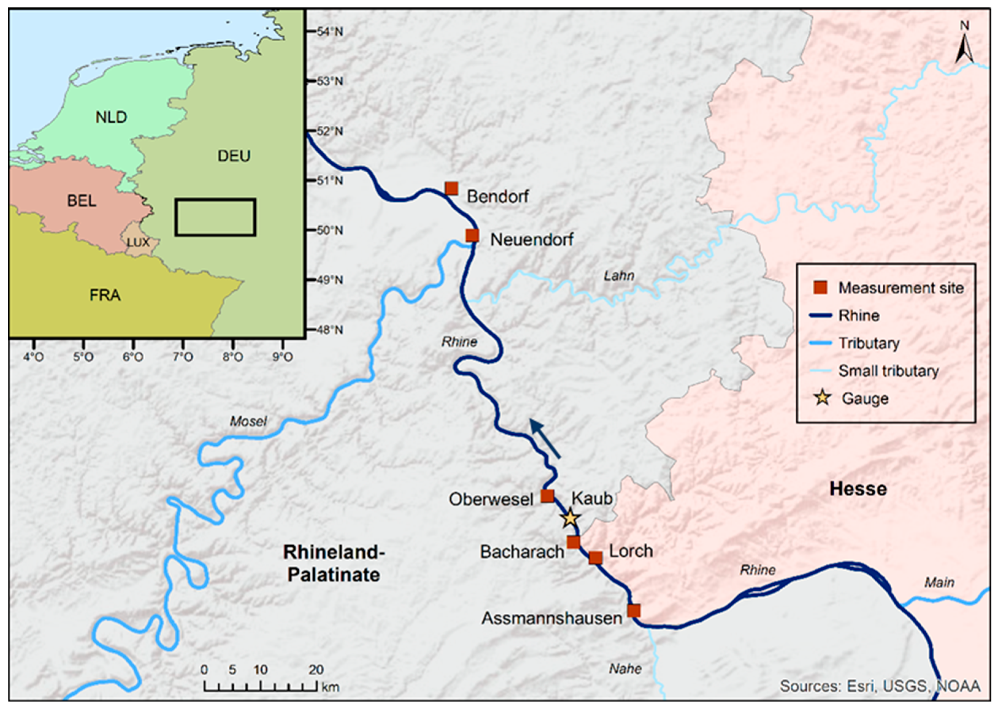
The Rhine River is one of the largest rivers in Europe, with a total length of 1230 km, a drainage basin of 185,000 km² [21,22], and an average discharge of 1640 m³/s at Kaub (Figure 1), located within the studied section [23]. The Rhine originates in the Swiss Alps at an altitude of 2345 m above sea level and reaches the North Sea at Rotterdam [24]. As a large gravel-bed river, it is representative for most of the German Federal waterways, e.g., Donau or Elbe, as they are similar in bed structure, width, depth, transport capacity and tributary influence.

The sampling sites of this study are located within the free-flowing middle Rhine section between Assmannshausen (Rh-km 532.9) and Bendorf (Rh-km 600.0). This section is characterized by the strongly incised valley of the Middle Rhine, cutting into the uplifted Devonian bedrock. The riverbed consists of Devonian bedrock exposure, partially covered with thin layers of alluvium, consisting of sand and gravel with a mean size of 17 mm. The channel’s morphology is defined by a steep gradient (0.26 m/km), channel widths of around 300 m, and sharp meandering bedrock bends [22,27]. The total sediment flux is dominated by clay and silt. The total sediment flux between 1991 and 2010 at St. Goar, which is located within the measured reach (Rh-km 557), was on average 1.5 Mt/a. Clay and silt in the Middle Rhine mainly originate from the large tributaries Mosel (Rh-km 592.2) and Main (Rh-km 496.6) [22]. Within the studied section of the Rhine, there are also two smaller tributaries, Nahe (Rh-km 529.2) and Lahn (Rh-km 585.7), which affect the pattern of the suspended sediment here. The rivers Nahe and Mosel flow into the Rhine from its left side and the rivers Main and Lahn join the Rhine on its right side (Figure 1).

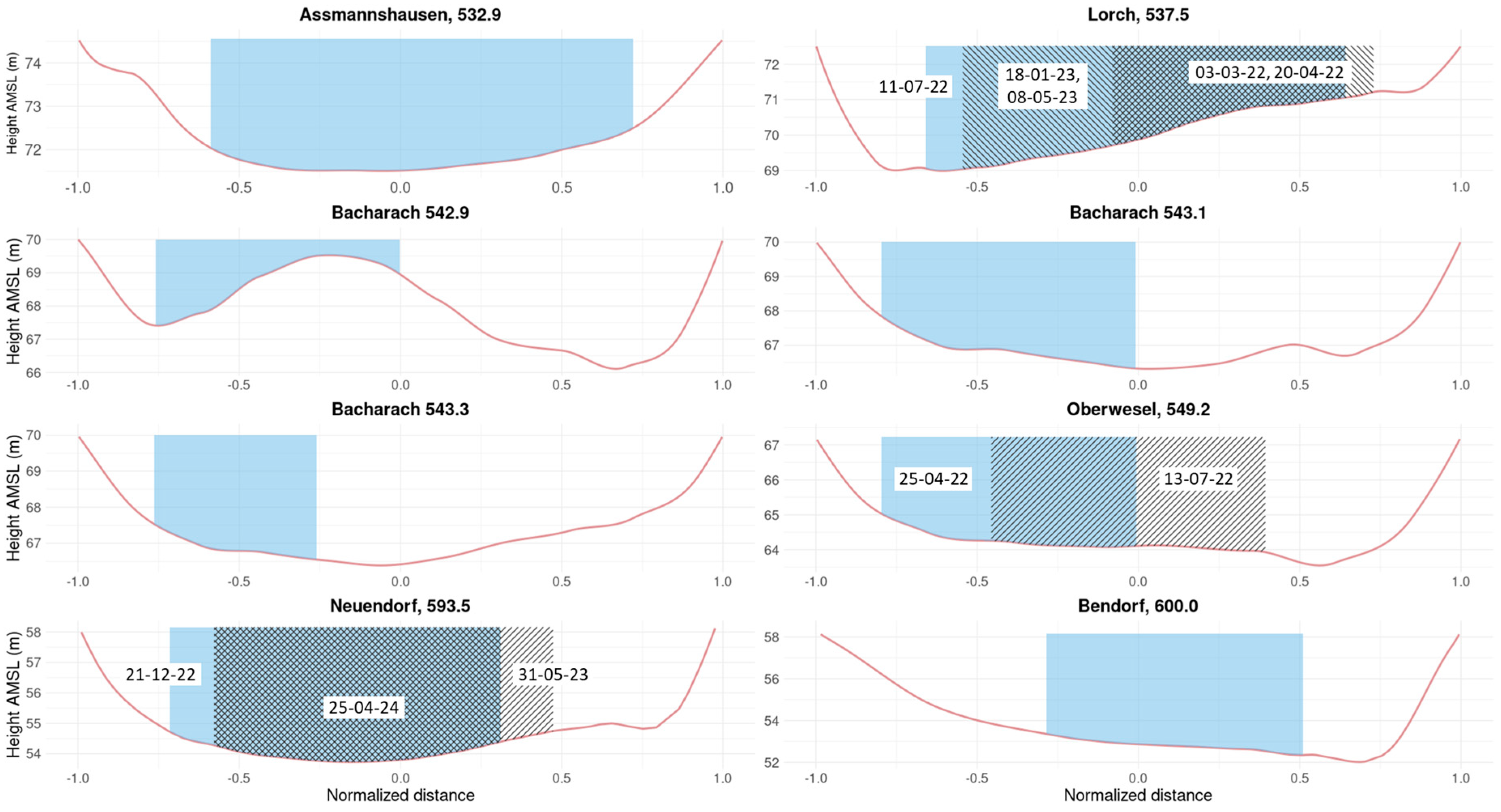
The channel morphology of the Rhine River for the different measurement sites is depicted in Figure 2. It can be characterized as symmetrical and U-shaped for the study sites Assmannshausen and Bacharach (543.3, 2 March 2022) and U-shaped with slight asymmetries for Bacharach (543.1, 11 May 2023), Oberwesel and Neuendorf. The riverbed at Bendorf is slightly, and at Lorch more strongly, skewed, with the deepest section of the river located towards the right bank at Bendorf and towards the left bank at Lorch. The channel cross-section at Bacharach (542.9, 10 May 2023) is W-shaped, with a shallow part located close to the center, between two deeper parts. Concerning the plan view of the river, all of the measurement sites except Bacharach are located downstream of a straight stretch. The three different measurement sites at Bacharach are located shortly upstream and within a slight right curve. The river width is slightly narrower at Oberwesel, measuring at 268 m compared to the other measurement sites that range between 328 and 411 m in width.

3. Materials and Methods

3.1. Data Collection

Measurement campaigns took place during low, average and high discharge conditions. We measured SSC using 1 L water samples and measured turbidity using the YSI turbidity sensor mounted onto the Exo3 sensor platform (Yellow Springs Instrument (YSI) Inc., Yellow Springs, OH, USA), together with YSI sensors for the temperature and electrical conductivity. Additionally, acoustic SSC measurements were taken using the acoustic backscatter sensor (ABS) LISST-ABS (Sequoia Scientific, Inc., Bellevue, Washington, USA), and a LISST-200X (Sequoia Scientific, Inc., Bellevue, WA, USA) was deployed to measure the in situ particle size distribution (PSD) during the nine campaigns. All instruments were simultaneously deployed from a vessel of the German Waterways and Shipping Authority (WSV). The turbidity and acoustic sensors were placed on a mounting device situated approximately 10 cm above the inlet of a water pump, which delivered 1 L water samples. Both the pump and the attached sensors, as well as the LISST-200X, were fixed to cranes, allowing for sampling at defined depths throughout the water column. A 100 kg weight was attached to each crane to ensure vertical deployment of the probes. This experimental setup was used to measure 15 river cross-sections of the Rhine River at six locations (Figure 1) over the course of 2.5 years, between 2022 and 2024, and yielded a total number of 495 water samples with corresponding sensor data. Due to time constraints during sampling, sufficient river depth required for the vessel, and the large amount of cargo ships cruising along the Rhine, it was not possible to cover the full cross-section at the sampling sites, and lateral coverage varied among the sites, as well as among campaigns (Figure 2). Throughout this paper, lateral positions are therefore presented as locations from −1 to 1, ranging from the left to right riverbank, respectively.

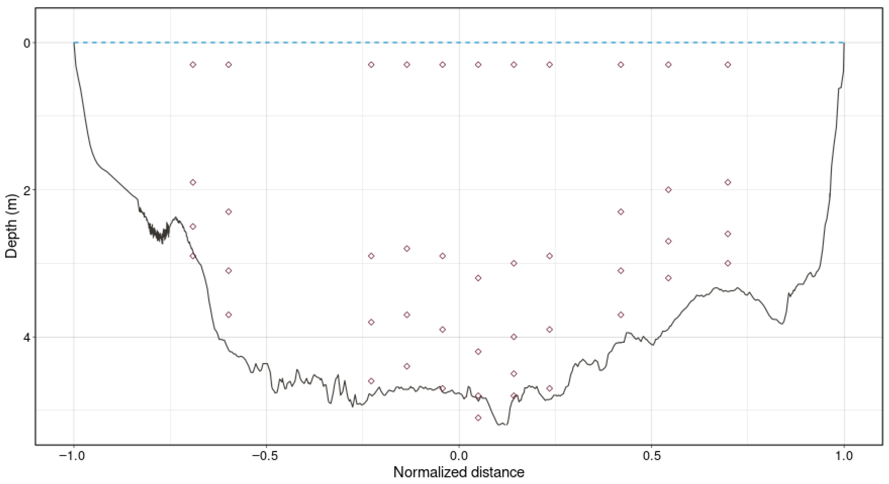
For vertical sampling, we took a surface sample at each vertical at 0.3 m below the water surface, depth samples at 60, 80 and 95% depth for verticals with a water depth of less than 5 m and additionally, a sample at 90% water depth for verticals with depths larger than 5 m (Figure 3), arguing that vertical SSC gradients are strongest towards the river bed. Additionally, we took 50 L pump samples, sieved with a 63 µm sieve, in eight campaigns, to measure the suspended sand concentrations.

We took a 1 L water sample at each depth by pumping the water through a hose with a 15 mm diameter at a rate of approximately 12 L per minute. The turbidity, temperature, electrical conductivity and acoustic sensors measured at a frequency of 1 Hz. They were attached to the pump and held constant at the same depth for approximately 30–90 s. To maximize the signal-to-noise ratio of the sensors, we then calculated the average of the sensor data collected at each depth, corresponding to the SSC from one water sample. The SSC was obtained by filtering the water samples in the laboratory through cellulose acetate filters of mesh size 0.45 µm. Between sampling and filtration, samples were kept cool and dark. The averaged turbidity values were related to the SSC from water samples, using linear regression analysis for each sampling campaign to translate turbidity in FNU to SSC in mg/L (SSC_turb). Averaged ABS values were calibrated in the same way (SSC_ABS). Temperature and electrical conductivity measurements were obtained as additional information to interpret differences in SSC, especially in the context of water mass origin and the lateral distinction of water masses, respectively. The in situ PSD data were obtained in a similar fashion, by lowering the LISST-200X to the desired depths and averaging the data with a frequency of 1 Hz, gathered for 30–90 s. The instrument measures 36 size ranges from 1.0 to 500 µm, from which the median particle size d₅₀ was calculated and is used as a representative particle size throughout this paper. Additionally, we obtained the ADCP data during six of the fifteen campaigns to analyze the vertical velocity distributions. We used an TRDI RiverPro 1200 (Teledyne RD Instruments, Poway, CA, USA) at a measurement frequency of 1 Hz, with an automatic dynamic bin size configuration of either 12 or 24 cm, depending on the water depth and flow velocity. It was attached to a trimaran and deployed upstream of the water pump and sensors for the full duration of sampling at each vertical (approximately 15 min). By averaging the data for each vertical bin over time, we obtained one robust vertical velocity profile for each sampled vertical.

3.2. Vertical and Lateral Data Analysis

We calculated $Ro$ by using its definition in Equation (2), based on the settling velocity ($w$) and the shear velocity ($u_{*}$) [16]. Therefore, we estimated $u_{*}$ by the linear fitting of the log-transformed law of the wall, based on the ADCP measurements [28]:

$$ln\left(z\right)=ln\left(z_0\right)+{\displaystyle \frac{\kappa }{u_{*}}}u\left(z\right)$$

(3)

where $u\left(z\right)$ is the velocity at point $z$ above the riverbed, $z_0$ is the height above the riverbed where $u=0$ and $\kappa$ is the von Karman constant. To evaluate the validity of these results, we compared them against values obtained from a calibrated hydrodynamic 1D numerical model (SOBEK, [29]) and from estimates based on the flow depth and water-surface slope. Both comparisons showed good agreement (see Supplementary Materials).

The settling velocity was calculated, assuming the particle density ${\rho }_s$ was that of quartz (2650 kg/m³) with a spherical shape [30]:

$$w={\displaystyle \frac{Rg{d}_{50}^2}{C_{1}v+\sqrt{\left(0.75C_{2}Rg{d}_{50}^3\right)}}}$$

(4)

where $R={(\rho }_s-{\rho }_w)/{\rho }_w$ is the particles’ submerged specific gravity (1.65 for quartz in water), $g$ is the gravitational acceleration and $d_{50}$ is the median particle diameter, which we derived from LISST-200X. $v$ is the kinematic viscosity of the fluid and $C_1$ and $C_2$ are constants set to 18 and 0.4 [30]. Additionally, we derived the Rouse number by fitting the vertical measurements of the SSC. This is performed using non-linear least square regression (nls) in R [31] of the form:

$$SSC~C_a\ast {z_a}^{Ro}$$

(5)

where $SSC$ is the measured concentration (mg/L) based on water samples (${Ro}_{fit,SSC})$, the averaged calibrated turbidity (${Ro}_{fit,SSC\left(turb\right)})$, or the averaged ABS measurements (${Ro}_{fit,SSC\left(ABS\right)})$. Both regression coefficients, $C_a$ and $Ro$, are calculated to optimally fit the measured SSC values. We calculated the residuals, i.e., the difference between the measured values and the fitted ideal Rouse curves, to see which measurement method yields the results with the least deviations from the theoretically assumed vertical SPM distribution. The method with the least deviations (${Ro}_{fit,SSC\left(turb\right)})$ was then used for further analyses, such as comparison to ${Ro}_{calc}$, based on theory (Equations (2)–(4)) and ${Ro}_{fit,sand}$, derived from the 50 L samples.

Since suspended matter is transported as aggregates and flocs [11,12], our assumption that SPM particles have a density of 2650 kg/m³ is only a rough approximation. Furthermore, in situ grain size measurements obtained from the LISST-200X yield the apparent diameter of the aggregated/flocculated particles. Consequently, Rouse numbers derived from the (in situ) grain size estimate and the assumed density of the primary mineral particles will overestimate ${Ro}_{calc}$. To address this, we reduced the density in Equation (4) so that ${Ro}_{calc}$ equals (${Ro}_{fit,SSC\left(turb\right)})$. We argue that the resulting density is the effective in situ density of the aggregated/flocculated particles.

In addition to the vertical Rouse analysis, we analyzed whether or not significant trends occurred laterally. We used linear least squares regression to calculate the lateral SSC and additional sensor data gradients. To compare these lateral gradients with gradients along the verticals, we additionally calculated vertical gradients of SSC and sensor data, either linearly or logarithmically, whichever represented the data more accurately, and calculated the steepness of the detected significant lateral and vertical trends, i.e., the change in parameter value per meter. Additionally, we calculated the ratios of the surface measurement of each vertical to the mean value of the corresponding vertical to approximate the representativeness of the surface measurements for the whole water column. Analogously, we calculated ratios for the mean values of the leftmost and rightmost measured verticals to approximate the relative lateral differences within the measured parts of the cross-sections.

Also, we calculated suspended sediment loads based on the full set of water samples taken within a campaign as a reference and compared them to loads calculated based on different methods, in order to improve the efficiency of the water sampling for the load calculations. We calculated loads based on the full cross-sectional data of SSC_turb and SSC_ABS, as well as based on surface samples taken close to the river bank, i.e., not further away from the bank than 20% of the river’s width (surface bank); from the average of surface samples at the leftmost and rightmost vertical (surface left/right), i.e., spanning the largest possible distance over the cross-section between sampling points; and the surface samples located closest to the center of the river with a maximum offset in each direction of 10% of the river’s width (surface center). Loads were calculated by multiplying the average SSC value for each distinct method and the discharge at the measurement time and location.

4. Results and Discussion

This section is structured to sequentially present and discuss the results of each research question outlined in Section 1.

4.1. Comparison of Measurement Methods

The complete dataset for turbidity shows a high linear correlation with the measured SSC from the water samples (Figure 4a, 14 campaigns, n = 380, R² = 0.94). This correlation of the entire dataset is substantially larger than the average correlations of the single campaigns (R² = 0.54). For ABS, the correlations among campaigns vary more strongly and the R² of the whole dataset (Figure 4b, 12 campaigns, n = 252, R² = 0.45) is substantially smaller than for separate correlations for each campaign (R² = 0.55). When comparing ABS and turbidity (Figure 4c), the data of the whole dataset correlates with an R² of 0.42, while the average R² value for single campaigns is 0.78.

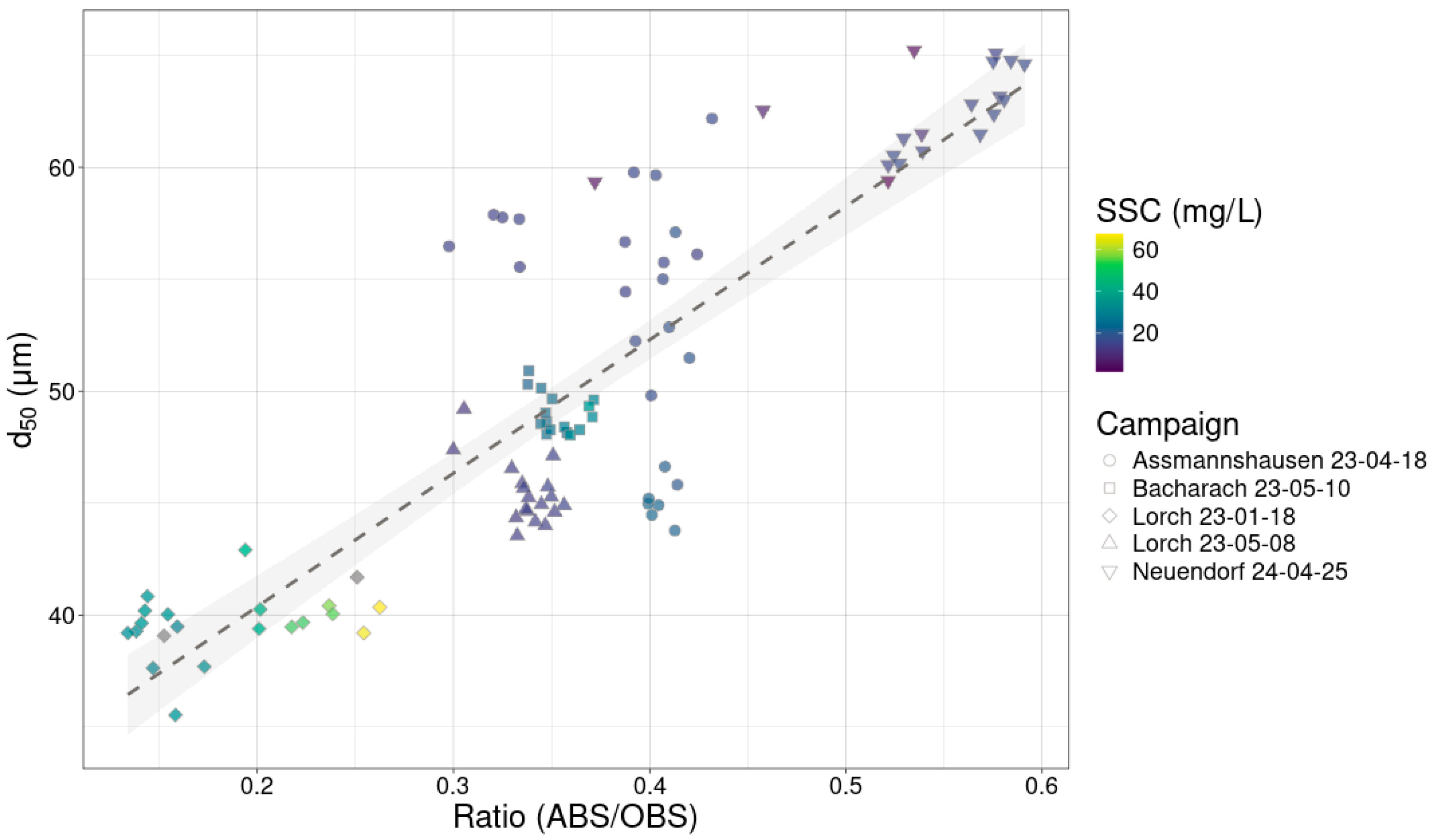
Based on the turbidity and ABS measurements in Figure 4c, there are three distinguishable clusters containing (I) the Lorch (3 March 2022), Bacharach (2 March 2022), and Oberwesel (13 July 2022) campaigns, (II) the Assmannshausen (18 April 2023), Bacharach (10 May 2023), Lorch (20 April 2022 and 8 May 2023), Neuendorf (24 April 2025) and Oberwesel (25 April 2025) campaigns and (III) the Lorch (18 January 2023) campaign, which suggests that the interrelationship of the optic and acoustic signal to the SSC are modulated by the particle size. This is shown by the positive relationship of the ABS/Turbidity ratio as a function of the particle size in Figure 5 (R² = 0.75, p < 2.2 × 10⁻¹⁶).

Statistically significant vertical trends can be detected for 53% of verticals for the turbidity measurements, 42% for the ABS measurements and 16% for the water sample SSC data. For these detected trends, the gradient, i.e., change of unit per meter depth, is given in

Table 1. Aggregated vertical statistics.

Parameter	Tot. Nmb. of Verticals	Sign. Trend (%)	Depth Increase (%)	Depth Decrease (%)	Mean Gradient	Sd Gradient
Turbidity	127	67 (52.8)	95.5	4.5	0.155 FNU/m	0.072 FNU/m
Conductivity	139	36 (25.9)	50.0	50.0	1.466 µS/cm/m	1.588 µS/cm/m
ABS	103	43 (41.7)	100.0	0.0	0.044 mg/L/m	0.029 mg/L/m
SSC	116	18 (15.5)	94.4	5.6	0.91 mg/L/m	0.185 mg/L/m

. The table also indicates the direction of the trend, which is increasing in >90% of cases with increasing depth. Nevertheless, some verticals show an SSC distribution that is characterized by larger concentrations towards the surface that are statistically significant.

Our findings suggest that vertical differences in SSC are more easily detected with sensor data than with water samples alone. Here, the turbidity sensor is superior to the acoustic backscatter sensor, since the data are characterized by less scatter and therefore finer trends are detectable, and because most of the measured suspended sediment is fine-grained, i.e., more easily detected with an optical compared to an acoustic method. The average d₅₀ measured in situ of the whole dataset is 49.1 µm, with a minimum average value for the Lorch campaign (18 January 2023) of 39.4 µm and a maximum average value for the Neuendorf campaign (24 April 2025) of 62.5 µm, i.e., in the coarse silt range.

4.2. Applicability of the Rouse Equation

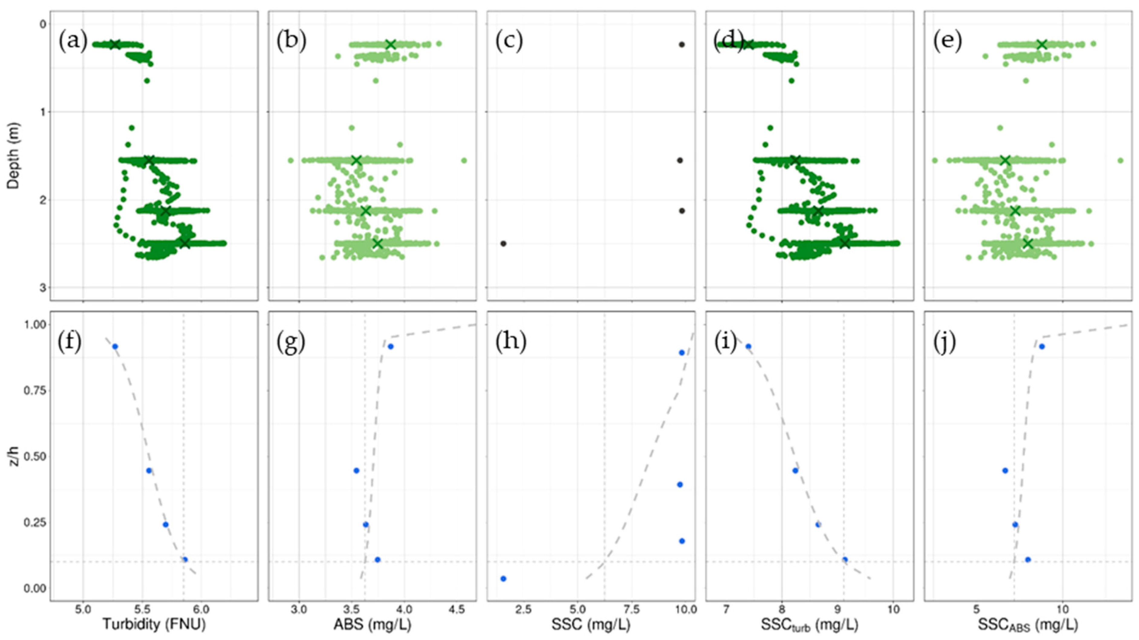
Figure 6 shows an example vertical, depicting the raw data and the process and influence of data averaging and sensor data calibration. Both the ABS and turbidity sensor data show substantial scatter in their single readings, with absolute differences of up to 1 FNU or 1 mg/L, respectively, within the measurement intervals at distinct depths (Figure 6a,b). Despite this scatter, data averaging enables us to detect vertical trends and calculate Rouse numbers. The same vertical that shows a positive ${Ro}_{fit,SSC\left(turb\right)}$ (0.047) shows a negative ${Ro}_{fit,SSC}$ (−0.13), which, in this case, mainly resulted from the deepest measured SSC being substantially smaller than the other water samples of the vertical. In contrast to the sensor readings (Figure 6a,b), the SSCs from water samples are derived from single measurements, with uncertainties in the order of 10–20% [7]. Variation in SSCs beyond this range of uncertainty and in contrast to the expectations from Rouse profiles, as depicted in Figure 6c, are frequently observed in our dataset and may result from short-term variations, e.g., due to turbulent mixing in river systems. The comparison with $Ro$, based on uncalibrated turbidity values (FNU), which is around half (0.023) of the ${Ro}_{fit,SSC\left(turb\right)}$ value, shows the importance of turbidity calibration before interpretation of the results is possible.

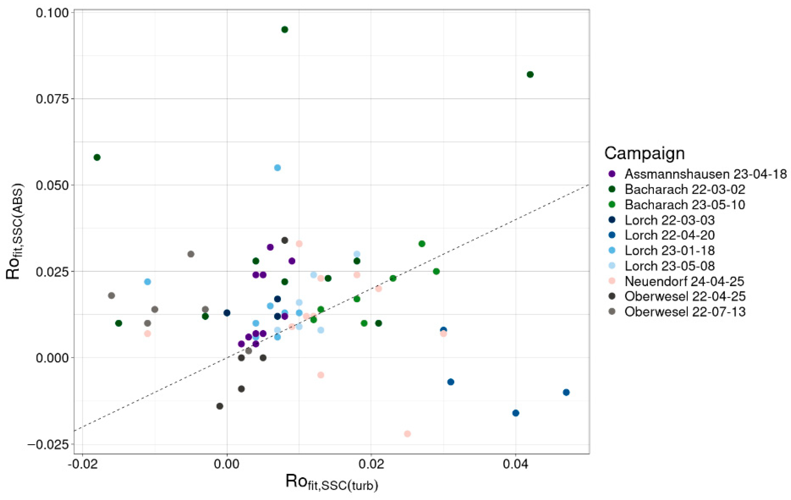
However, deviations of single SSC measurements in a vertical, as shown in Figure 6c, do not have a strong influence on SSC_turb and SSC_ABS, which are derived from the regression to SSC from water samples over the entire dataset of each sampling campaign. The calibrated turbidity in Figure 6i shows a vertical gradient, which can be well-fitted to a Rouse gradient. Nevertheless, the ABS data for this vertical shows that the sensor data might also produce negative values for $Ro$, when the absolute values differ very little with depth. This is a rarity in our dataset. The fitted $Ro$ are generally low, ranging from −0.26 to 0.25 for SSC, from −0.056 to 0.095 for ABS, from −0.016 to 0.047 for SSC_turb, and from −0.049 to 0.056 for SSC_ABS. None of the $Ro$ values show a correlation with the SSC. The vertical shown in Figure 6b is one of nine verticals in the entire dataset, which show negative ${Ro}_{fit,SSC\left(ABS\right)}$ values, i.e., representing 8.7% of all ABS verticals (n = 104). For ${Ro}_{fit,SSC\left(turb\right)}$, negative values were observed at ten verticals (n = 119, 8.4%), and for ${Ro}_{fit,SSC}$, at 15 verticals (n = 123, 12.2%).

Both ${Ro}_{fit,SSC\left(ABS\right)}$ and ${Ro}_{fit,SSC\left(turb\right)}$ show small absolute values (Figure 7). However, it is notable that the average value of ${Ro}_{fit,SSC\left(ABS\right)}$ (0.016) is an order of magnitude larger than the average value of ${Ro}_{fit,SSC\left(turb\right)}$ (8.5 × 10⁻³). This can be explained by the larger sensitivity of acoustic systems to larger grain sizes compared to optic systems [32], which are less uniformly distributed vertically. This can also be seen in Figure 5, where the ratio of ABS/OBS (turbidity), i.e., their sensitivity comparison, is larger for larger grain sizes. ${Ro}_{fit,sand}$, derived from the 51 vertical gradients of the suspended sand concentration (i.e., 50 L samples which were sieved with >63 µm) show an average value of 0.10 and range from −0.021 to 0.51. This is again an order of magnitude larger than ${Ro}_{fit,SSC\left(ABS\right)}$, indicating that ${Ro}_{fit,SSC\left(ABS\right)}$ is affected by the mixture of the fine (i.e., clay/silt) and sand fractions. The later represents, on average, 9% of the total suspended solids [22].

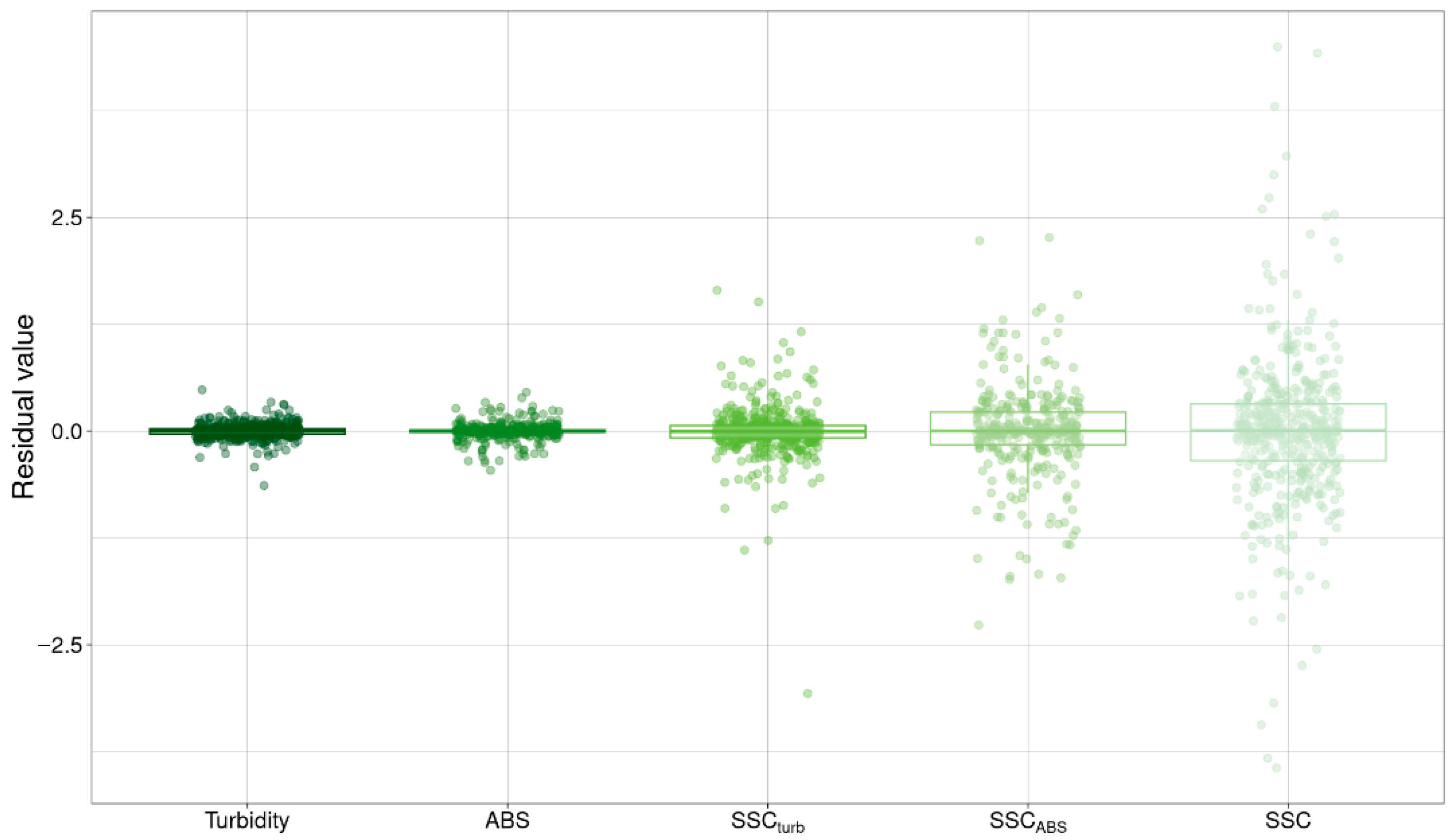
The residual values, i.e., the difference between the measured value and corresponding value of the fitted Rouse profile, for the sensor data are consistently smaller compared to the residuals of the water samples with the average absolute values of 0.052 and 0.048 for turbidity and ABS, respectively. The average absolute value for residuals based on the SSC from water samples is an order of magnitude larger (0.55). Standard deviations are 0.08 for residuals based on turbidity, 0.09 for ABS and 0.88 for SSC from water samples. The residual values for the SSC_turb and SSC_ABS are in the same order of magnitude as for SSC, with an average of absolute values of 0.15 for SSC_turb with a standard deviation of 0.29 and an average absolute value of 0.33 for SSC_ABS with a standard deviation of 0.53. The larger standard deviations of the calibrated sensor data are due to the scatter, introduced by the calibration with water samples. Nevertheless, the SSC_turb is characterized by substantially smaller residual scatter than the SSC from water samples, indicating that the SSC_turb is closer to the expected Rouse distribution than the SSC from water samples (Figure 8). For this reason, it is used as the base parameter, ${Ro}_{fit,SSC\left(turb\right)}$, in the following analyses.

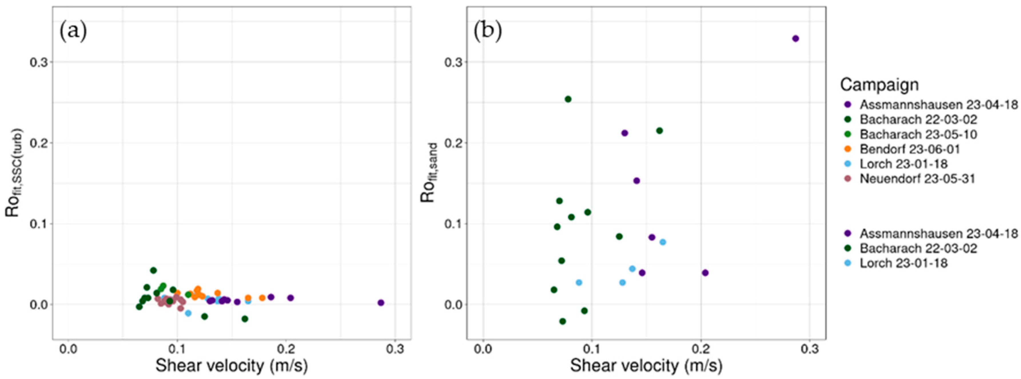
Values of ${Ro}_{fit,SSC\left(turb\right)}$ for the fine fraction vary significantly among several campaigns, with variability within the cross-section during a single campaign being much smaller than between campaigns (Figure 9a). For the sand fraction, Kruskal–Wallis testing (p = 0.01) and post hoc testing, using the Bonferroni correction method (p = 0.01), reveal significant differences, only between the Lorch (11 July 22) and Oberwesel (25 April 2025) campaigns. Among all other campaigns, no significant differences could be found, i.e., the scatter within single campaigns is larger than the differences among campaigns (Figure 9b).

${Ro}_{fit,SSC\left(turb\right)}$ shows no correlation (R² = 0.03, p = 0.13), while ${Ro}_{fit,sand}$ shows a small positive correlation (R² = 0.16, p = 0.04) with shear velocity, which varied between 0.07 and 0.28 with an average value of 0.12 (Figure 10).

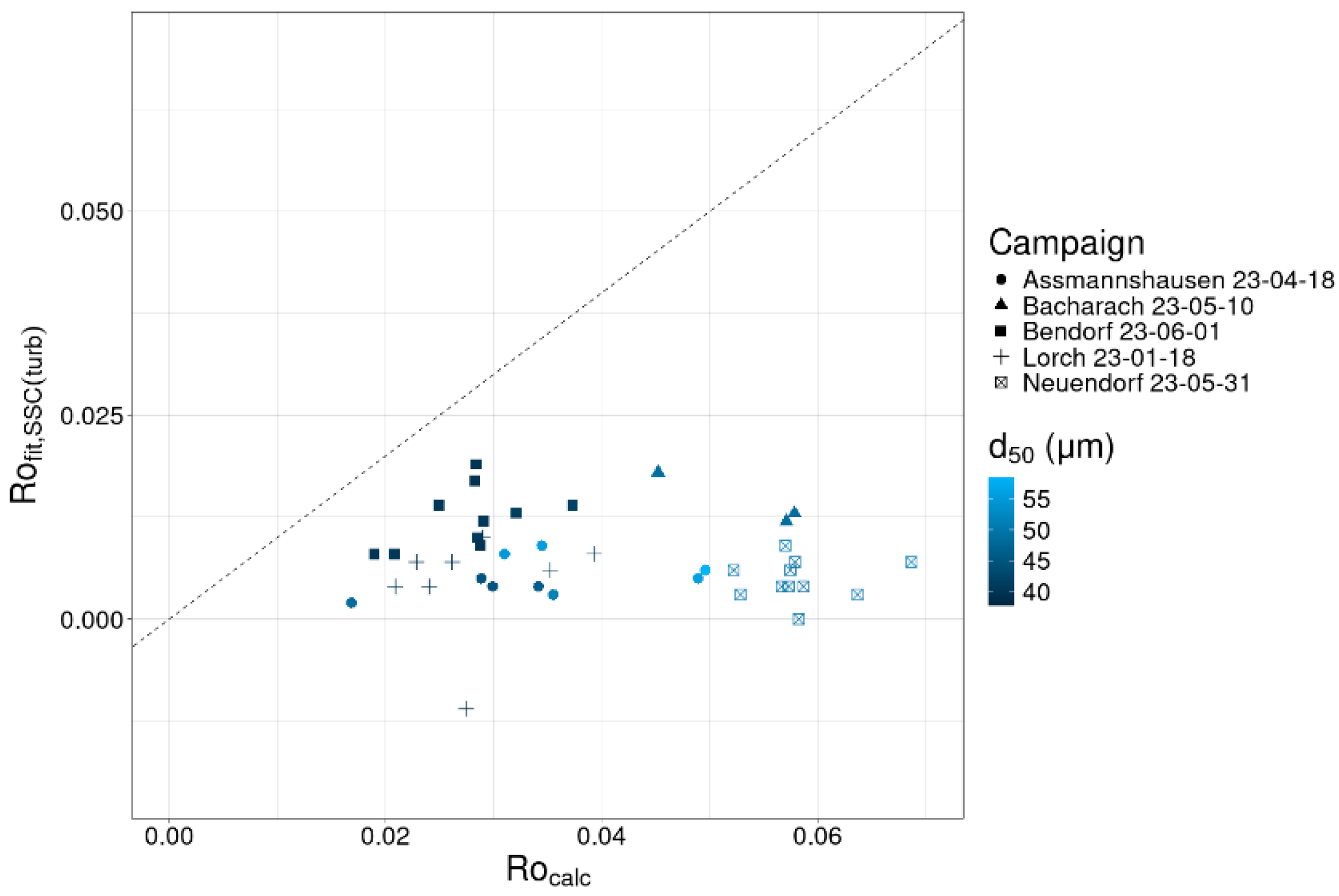
Rouse values calculated from Equation (2) (${Ro}_{calc}$) range from 0.017 to 0.069 and are, without exception, larger than those derived from fitted vertical gradients (${Ro}_{fit}$), which typically range between 0 and 0.025. As expected, ${Ro}_{calc}$ increases with d₅₀ with maximum values close to 0.07 (Figure 11). This theoretically derived dependency on particle size is not visible in the fitted data, which shows no correlation between d₅₀ and ${Ro}_{fit,SSC\left(turb\right)}$ (R² = −0.01). When comparing ${Ro}_{calc}$ with ${Ro}_{fit,SSC\left(turb\right)}$, smaller d₅₀ values tend to be closer to the theoretical values than the larger values of d₅₀; albeit, they are still smaller than theoretically expected when calculated with an assumed density of 2650 kg/m³. The absolute difference between ${Ro}_{fit,SSC\left(turb\right)}$ and ${Ro}_{calc}$ does significantly correlate with d₅₀ (R² = 0.47, p = 4.1 × 10⁻⁷). This derivation indicates that larger particle sizes may show a higher degree of flocculation, i.e., their density values are further away from the expectations for primary particles.

Thus, effective particle densities within the waterbody are likely lower than the usually assumed density of quartz (Figure 12). Adopting the density in Equations (2) and (3) such that ${Ro}_{calc}={Ro}_{fit,SSC\left(turb\right)}$ results in a mean effective density value of the 41 analyzed verticals of 1367 kg/m³ with a minimum value of 1000 kg/m³, which is the calculation minimum, due to the calculation procedure of submerged specific gravity and a maximum value of 2100 kg/m³, which is still substantially smaller than the density of quartz. Effective densities for Assmannshausen, Bacharach, Lorch and Neuendorf do not differ significantly, while Kruskal–Wallis (p = 5 × 10⁻⁶) and post hoc testing with Bonferroni correction shows significant differences between the campaign at Bendorf and the campaigns at Assmannshausen and Neuendorf, which are characterized by smaller densities (Figure 12a). The larger densities at Bendorf can be explained by significantly smaller particle sizes, with an average d₅₀ of 40.4 µm compared to 52.2 µm at Assmannshausen and 50.8 µm at Neuendorf. Since the measurements at Neuendorf and Bendorf are separated by only 7 km and have water level differences of 7 cm, hydrological reasons for these particle size differences are implausible. More likely, the difference in particle size is due to the turbulent breakup of flocs along the flow path between the two sites or due to the mobilization of different material. This section of the river contains two elongated islands (approximately 4 km and 2 km in length), which divide the flow three ways just upstream of the measurement site at Bendorf. This increases turbulence and may serve as an additional source of suspended matter. Also, similar particle sizes were measured at Lorch (18 January 2023, with an average d₅₀ of 39.4 µm. Here, however, values of ${Ro}_{fit,SSC\left(turb\right)}$ were significantly lower than at Bendorf (p = 0.017), with no differences in shear velocities, indicating differences in mineral composition.

Laterally, none of the campaigns show any patterns (Figure 12b), except for Bacharach (10 May 2023), which shows a lateral pattern that is similar to that of the lateral conductivity measurements of this campaign (Figure 13), indicating that the lateral differences in effective density here may stem from the SPM originating from different water masses. However, the correlation between the density and conductivity is not significant (R² = 0.94, p = 0.11) and is only based on three data points.

We expected minimal vertical differences in SSC, since the sampling sites are usually dominated by particle sizes in the silt range that have often been reported to be transported as a well-mixed wash load [33]. This is confirmed by the in situ PSD measurements with an averaged d₅₀ of 49.1 µm, i.e., coarse silt. However, even though the suspended load is dominated by small particles (mainly silt), full vertical mixing is not always given. This extends the findings of, e.g., Bungartz et al. (2006), Lamb et al. (2020), and Nghiem et al. (2022), who calculated increased settling velocities for clay and silt-sized particles due to flocculation, resulting in vertical concentration differences [12,34,35]. The discrepancy of the expected theoretical density and the calculated apparent, effective density also points towards flocculation within the system, although our in situ PSD measurements show that possible flocculation of primary particles hardly results in flocs above the silt range. This is in accordance with studies analyzing the influence of turbulence and shear-stress on floc formation, finding that turbulence helps in the formation of flocs to a certain degree but prevents the formation of larger flocs [34,35,36].

Despite outliers in SSC, the calibrated turbidity is still suitable to detect fine vertical differences. The data are robust, since the calibration is performed based on the average turbidity values and the SSC values of the whole campaigns. This finding is backed up by the residual analysis of Rouse distributions. Here, the sensor data consistently shows residual values an order of magnitude smaller than those of the water sample-based SSC measurements. Therefore, the Rouse analysis again stresses the uncertainties connected to analyses based solely on water samples, and in general, our results emphasize the added value that surrogate sensor measurements provide to detect subtle differences within rivers for an improved understanding of suspended sediment transport in the system.

The Rouse theory holds up in most cases, although our results show that in some circumstances, as presented in this study, i.e., particles sizes primarily in the silt range, low SSC, and when shear velocities are constantly large enough to keep the transported matter suspended, the Rouse framework reaches its limits and loses its predictive capacity. In general, the detected values for $Ro$ are very small, with some verticals showing larger concentrations towards the surface, i.e., ${Ro}_{fit}<0$. Therefore, using calculated Rouse gradients based on Equations (1) and (2) when extrapolating from surface measurements to deeper parts of the water column would lead to a substantial overestimation of SPM towards the bed, and to large errors in load calculations. This shows that predicting Rouse gradients is generally limited by the unknown transport conditions and properties of the suspended sediments in rivers, highlighting the importance of in situ measurements for an improved understanding of conditions for suspended sediment transport and accurate load estimations. Here, turbulence is consistently large enough to suspend and vertically mix not only the main particle size fraction of coarse silt but also sand and larger-sized particles, as can be deduced by the generally low values of $Ro$ for both ${Ro}_{fit,SSC\left(turb\right)}$ and ${Ro}_{fit,sand}$. However, there is a significant but small positive correlation between shear velocity and ${Ro}_{fit,sand}$, indicating that the vertical distribution of this fraction is less homogenous for larger shear velocities. This suggests that higher shear velocities mobilize more sand particles that remain predominantly concentrated near the bed. Additionally, this may hint that increasing shear stress may mobilize coarser grain sizes that are otherwise immobile under a flow with smaller shear velocities, i.e., representative of a shift in transported grain size distribution.

4.3. Lateral SSC Distribution

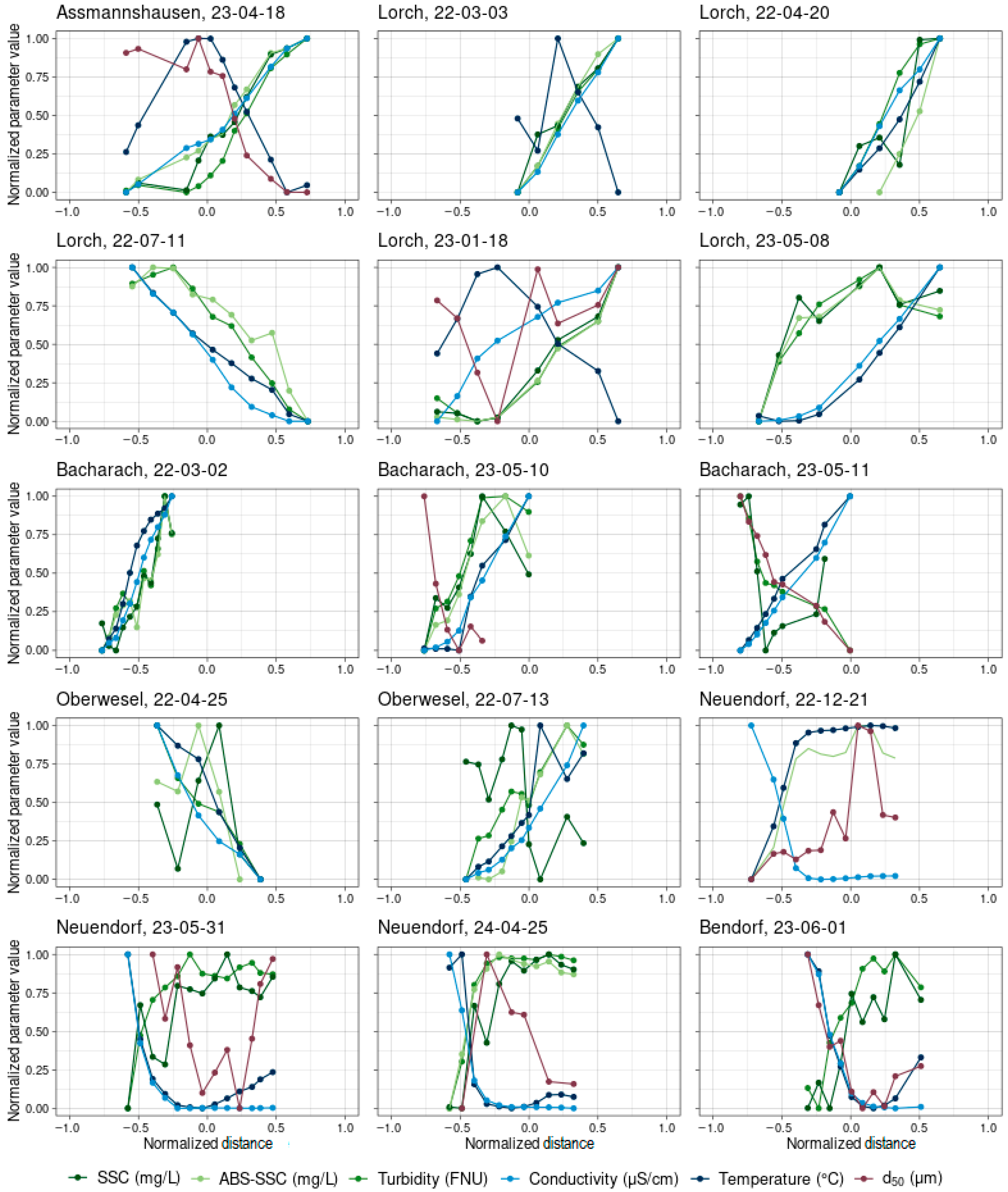
Significant lateral trends were detected within every campaign, at least for some parameters (Figure 13). If trends are visible for the SSC, turbidity and acoustic backscatter, they always follow the same direction. This is also true for conductivity for every campaign upstream of the Mosel tributary, except for Bacharach (11 May 2023). Downstream of the Mosel tributary, the trend of conductivity always opposes that of SSC and turbidity and acoustic backscatter, indicating the influence of the Mosel tributary on lateral gradients. Four types of trend curves can be observed: (i) a linear trend, e.g., Bacharach (2 March 2022) or Lorch (3 March 2022), (ii) a strong local gradient at some point along the cross-section with more or less constant values to the left and right of that, (iii) a mixture of type (i) and (ii), e.g., Lorch (18 January 2023, 8 May 2023) and (iv) no trend. Type (ii) gradients are especially observable for sampling sites that are closely downstream of tributaries, e.g., Neuendorf (31 May 2023) and Bendorf (1 June 2023). Type (iii) is characterized by a slowly increasing or decreasing gradient over the cross-section and smaller parts with constant values towards one side of the measured cross-sectional width, e.g., Lorch (8 May 2023). Type IV (no trends) is not observable for whole campaigns, but rather for single parameters. Especially temperature and d₅₀ tend to show variable patterns along the cross-section, e.g., Assmannshausen (18 April 2023) and Lorch (18 January 2023), but also SSC, e.g., Oberwesel (13 July 2022) and Bacharach (11 May 2023). Temperature, in general, shows very little variation along the cross-section, with differences between the leftmost and rightmost measured vertical always being below 1 °C. Since it can be altered by sunlight, ship traffic and its proximity to the banks, it is prone to show patterns differing from the other, more inherent water parameters. The large degree of variation within the d₅₀ curves is probably due to high scatter in the data. When the single LISST-200X measurements are not disturbed, information about d₅₀ offers an important means to understand underlying processes within a river cross-section. But since they are rather easily disturbed, due to environmental or mechanical disturbances such as air bubbles, thermal microstructures, obstruction of the beam path or improper positioning due to flow disturbances [37], the presented statistics for the cross-sections only consider the parameters of acoustic backscatter, turbidity, SSC and conductivity.

Seven of fifteen campaigns show linear trends (type i) for at least one parameter, making it the most common trend in our dataset. Linear trends indicate that sampling took place over a part of the cross-section that lies within a mixing zone, since the parameters consistently increase or decrease towards one site but do not reach a plateau. We argue that these changes are due to the mixing of different water bodies and not due to shifts in SSC-maxima due to curvature, since conductivity changes in corresponding patterns. However, as the different campaigns at the sampling site Lorch illustrate, these trends can vary over time. Here, three of the five campaigns show a type (i) while the others show type (iii) trends, characterized by a slowly increasing or decreasing gradient over the cross-section and smaller parts with constant values towards one side of the measured cross-sectional width, indicating that the type of lateral trend may change under different conditions. Type (ii) trends, which show a break-point behavior, are mostly restricted to the sampling sites Neuendorf and Bendorf that lie 1.3 Rh-km and 7.8 Rh-km, respectively, downstream of the confluence of Mosel and Rhine, and therefore, closely downstream from the confluence of two large rivers. At Neuendorf, the influence of the tributary Mosel is visible by the very strong lateral gradient around −0.5 normalized distance, i.e., 250 m from the right bank, marking the border between the two water masses of Mosel and Rhine. This is consistent for each campaign and parameter (except d₅₀) measured here. For Bendorf, the strong lateral transition is less pronounced and shifted further to the right side of the river around −0.1 normalized distance, indicating that the mixing of the two water masses has progressed further.

When considering the scatter of the data, conductivity is the most consistent parameter for measuring lateral variability, which is likely due to different water masses along the cross-section. In some cases, like Assmannshausen, conductivity shows the same lateral pattern as SSC. However, it is prone to changes that are independent of the SSC distribution, illustrated by the two campaigns at Bacharach, separated by one day, where the direction of the lateral conductivity trend inverses (10–11 May 2023). The reason for this is presumably a shift in the water mass origin, since the discharge increased from 2100 to 2300 m³/s overnight. Also, downstream of the confluence of the Mosel, conductivity consistently opposes the lateral trends of the SSC. Therefore, it cannot be used as a means to approximate the SSC, but it can serve as a reliable means to gauge lateral mixing of two water masses downstream of confluences.

The turbidity and acoustic backscatter sensors follow the lateral trends of SSC at every campaign and even detect significant lateral trends when there are none detectable via water samples, as can be seen at the campaign at Oberwesel (Figure 13). Acoustic backscatter and turbidity correlate with the SSC, with an R² > 0.5 for every campaign except for the two campaigns at Oberwesel (

Table 2. R² values of linear regression for the parameters of acoustic backscatter, turbidity and conductivity to SSC.

Campaign	R2 Acoustic BS	R2 Turbidity	R2 Conductivity
Assmannshausen 18 April 2023	0.97	0.95	0.94
Lorch 3 March 2022	0.95	0.96	0.95
Lorch 20 April 2022	0.67	0.65	0.69
Lorch 22 July 2022	–	–	–
Lorch 18 Jaunary 2023	1.00	0.99	0.72
Lorch 8 May 2023	0.98	0.93	0.34
Bacharach 2 March 2022	0.86	0.85	0.86
Bacharach 10 May 2023	0.84	0.85	0.35
Bacharach 11 May 2023	–	0.60	0.14
Oberwesel 25 April 2022	0.39	0.10	0.02
Oberwesel 13 July 2022	0.27	0.21	0.35
Neuendorf 22 December 2022	–	–	–
Neuendorf 31 May 2023	–	0.57	0.58
Neuendorf 25 April 2024	0.78	0.82	0.81
Bendorf 1 J une 2023	–	0.69	0.72

), which are characterized by very noisy water sample SSC data. As in the case of vertical trends, the turbidity sensor is also superior to the acoustic backscatter sensor in the detection of significant lateral trends, due to less scatter in the data and a larger percentage of fines in the SPM.

The leftmost and rightmost measured verticals showed ratios of 0.75 for turbidity, 0.72 for the water sample’s SSC, and 0.67 for acoustic backscatter, i.e., relative differences of 25–33%, with relative changes in median particle sizes being substantially smaller (9%). Therefore, changes in the sensor data are probably due to changes in the SSC, rather than changes in particle sizes, which is also supported by the large differences in SSC of 6.5 mg/L between the leftmost and rightmost measured vertical, on average. This again emphasizes the large uncertainties introduced in the load calculations, based on the location of the water samples. The absolute differences for every campaign and parameter are shown in

Table 3. Absolute differences between averaged values of the leftmost and rightmost vertical of every campaign. Additionally, the distances between these verticals and the average values across all campaigns are given.

Campaign	Turbidity (FNU)	ABS-SSC (mg/L)	SSC (mg/L)	Conductivity (µS/cm)	d50 (µm)	Distance (m)
Assmannshausen 18 April 2023	4.08	2.13	9.42	54.84	13.20	225
Lorch 3 March 2022	5.12	0.15	6.62	19.90	NA	150
Lorch 20 April 2022	1.53	0.57	6.01	44.3	NA	150
Lorch 22 July 2022	1.29	0.03	NA	119.77	NA	270
Lorch 18 Jaunary 2023	14.93	5.931	33.24	53.37	0.57	270
Lorch 8 May 2023	0.63	0.48	2.33	76.00	4.23	270
Bacharach 2 March 2022	0.75	0.14	2.62	10.58	NA	100
Bacharach 10 May 2023	1.21	0.51	4.08	4.87	2.17	135
Bacharach 11 May 2023	5.12	NA	1.69	19.65	10.12	130
Oberwesel 25 April 2022	0.84	0.32	1.21	25.38	NA	100
Oberwesel 13 July 2022	0.76	0.02	1.92	57.33	NA	115
Neuendorf 22 December 2022	NA	0.11	NA	248.56	11.75	175
Neuendorf 31 May 2023	1.43	NA	2.89	147.26	0.02	175
Neuendorf 25 April 2024	2.01	1.92	10.06	184.63	0.65	150
Bendorf 1 J une 2023	0.55	NA	1.89	114.50	1.85	155
Average	2.87	1.03	6.46	78.73	4.95	170

.

Significant lateral trends are present for >90% of campaigns for ABS and turbidity data and for 70% of campaigns for SSC from water samples (

Table 4. Aggregated lateral statistics.

Parameter	Total No. of Campaigns	Significant Trend (%)	Increase Left to Right	Increase Right to Left	Mean Gradient
Turbidity	14	13 (92.9)	11	2	0.017 FNU/m
Conductivity	15	15 (100)	10	5	0.392 µS/cm/m
ABS	12	11 (91.7)	11	0	0.005 mg/L/m
SSC	13	9 (69.2)	9	0	0.044 mg/L/m

).

Lateral differences within our study are probably due to tributary influence and incomplete mixing of two water masses with different SSCs. This is evident when considering the lateral conductivity trends that always either follow or oppose the SSC trends, but are similar in strength, and how they change laterally. Conductivity shows considerably less fluctuation than SSC and the ratio among rivers is rather stable, with the conductivity of the Mosel being consistently larger than that of the Rhine River. Since differences in conductivity stem from different water mass origins, and since these differences are laterally significant within every measurement campaign, they must indicate incomplete mixing of two water bodies. This is in accordance with other studies, e.g., Böhme (2006), who found that the lateral distribution of conductivity in the river Elbe is influenced by tributaries of up to 185 km upstream of the measurement site and Lazo et al. (2024), who even used conductivity as a chemical tracer for flow partitioning in a mixing model [38,39].

During the campaigns at Bacharach, sampling was limited to the left half of the river’s cross-section, therefore missing data at the thalweg. This is also the case for the campaigns at Oberwesel, Lorch and Bendorf, albeit that here, data were gathered at the geometrical center of the cross-section. We acknowledge that due to the absence of data of the thalweg, which could not be sampled due to the constraints outlined in Section 3.1, the hydrodynamic conditions in the deepest part of these cross-sections remain unknown, which may weaken the results of the lateral SSC distribution. However, lateral patterns observed at these sites do not differ from those obtained during campaigns in which the thalweg was sampled. Therefore, these data gaps are not considered to undermine the general conclusions drawn from this study.

4.4. Implications for SPM Monitoring in Large River Systems

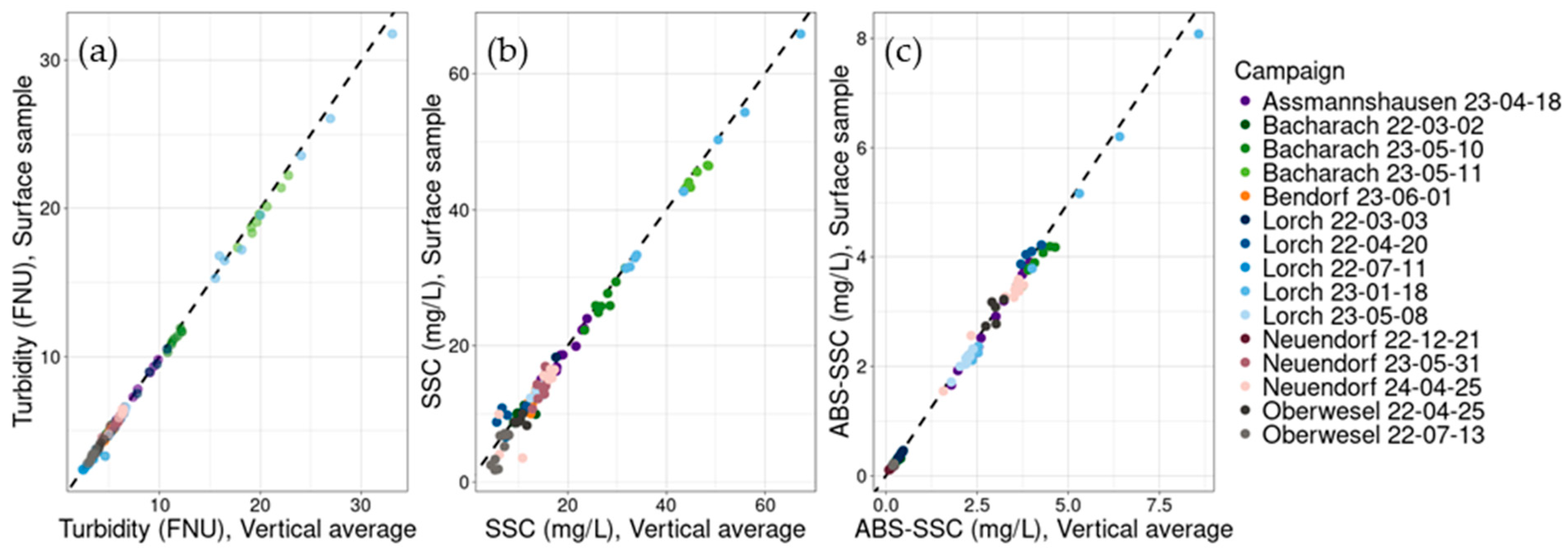
The overall small Rouse numbers are also reflected in the small difference between the surface SSC and the depth-averaged SSC values, as shown in Figure 14, where all points are plotted very close to the 1:1 line. Surface measurements from the water sample’s SSC, as well as for turbidity and ABS, underestimate the average concentrations by 3% for turbidity and ABS, and 5% for the water sample’s SSC. Surface measurements of the suspended sand yielded an average value of 78% compared to the average values of the complete verticals.

The comparison of the calculated loads, based on the full water sample dataset, multi-point calibrated turbidity and different surface sampling techniques, shows that loads calculated based on calibrated turbidity are hardly any different to the loads based on full cross-sectional water sampling. The largest errors occur due to lateral gradients and sampling only one location, close to the bank. However, taking two surface water samples from the verticals located furthest apart still introduces a larger error into the load calculations than a single surface water sample taken at the center of the river (Figure 15).

The spatial analysis highlights the importance of both the lateral and vertical gradients of suspended sediment within river channels. Our results reveal that the lateral gradients of suspended matter are typically an order of magnitude smaller than the vertical gradients. However, the total difference in sensor data and SSC between the left and right banks is an order of magnitude larger than that between the water surface and the channel’s bottom when extrapolating the data of the calculated gradients, due to the much larger distance over which these gradients apply. This observation is in accordance with findings in Slabon et al. (2025) [16]. Considering only the verticals that show a significant trend and multiplying their gradients with the average largest depth per campaign of 4.3 m yields the maximum differences between the surface and channel bottom of 0.67 FNU (turbidity), 0.19 mg/L (ABS) and 3.9 mg/L (water samples). This scenario, assuming the maximum depth throughout the dataset, as well as significant trends at every vertical, still yields smaller absolute results than the comparison of the average values of the leftmost and rightmost measured verticals. Considering that we were mostly only able to cover the central parts of the cross-sections, the lateral differences between the banks are likely to be even larger if considered for the full cross-section. An approximation can be calculated by multiplying the calculated lateral gradients, based on the trend analysis with the mean river width of our sampling sites of 350 m, yielding 5.95 FNU (turbidity), 1.75 mg/L (ABS) and 15.4 mg/L (SSC). Although this is probably an overestimation, it shows the limitations of point monitoring stations that are located only on one side and close to a riverbank, especially for calculating suspended sediment loads. On the other hand, our study shows that water properties measured at the surface do not differ much from the average conditions over the water column. This is shown by the vertical ratio analysis, the generally small detected Rouse numbers, and the RMSE analysis of load estimates, based on the surface samples. Our results therefore show that uncertainties introduced by a lateral sampling position are larger than the uncertainties introduced by assuming full vertical mixing, and hence, representative sampling at the surface. We suspect that this is true for all large rivers, such as the Rhine, where turbulence is usually strong enough to fully suspend and mix the transported particles vertically, as is shown by the non-existent correlation between the ${Ro}_{fit,SSC\left(turb\right)}$ values and the shear velocity. We therefore recommend sampling at the center of the river, rather than near the banks. Our results suggest that if only one sampling depth close to the surface is feasible, the results are still representative and additional sampling in larger depths adds little benefit for load calculations. Under these conditions, remote sensing tools, which mainly detect the water properties near the water surface, may also provide useful information for the large-scale SSC monitoring in rivers and may even be used to gauge the substantial lateral differences and include them in the annual load estimates [40,41,42].

However, our analyses also show that the suspended sand fraction behaves differently. We found a weak but significant positive correlation between ${Ro}_{fit,sand}$ and shear velocity, indicating that larger shear stresses lead to the transport of larger amounts of sand and larger particles close to the riverbed. Surface sampling therefore provides a cost-effective and reliable estimate for the fine fraction, which dominates the annual suspended load with 91%, and in terms of flux monitoring the underrepresentation of the sand fraction in surface samples, which still represent 78% of the average vertical value, is negligible [22]. Nevertheless, for research questions addressing riverbed morphodynamics, sediment sorting or storage and remobilization, the measurement of transported sand remains essential [43,44,45,46].

Recording the vertical variability of the SSC in flowing waters is only possible by using heavy weights, which prevent the measuring device from drifting with the current. These heavy weights in turn require the use of a powerful crane attached to a large vessel, which is expensive and requires a large crew. Our findings from the Rhine suggest that instead of relying on large crews and vessels to measure the vertical and lateral variability of the SSC in river cross-sections, turbidity sensors may offer a reliable alternative. Compared to traditional and labor-intensive SSC measurements from water samples, turbidity measurements are faster and show less scatter in the data. The statistical analysis shows that turbidity correlates well with SSC distributions across the entire dataset and is superior to water samples and acoustic backscatter in resolving both vertical and lateral differences. Under similar conditions, as observed in our study, i.e., large and turbulent rivers with low SSC and predominantly silt-sized particles, we argue that the measurement of turbidity that is close to the surface is sufficient and representative for the whole water column and calibration, with three to five water samples taken over the cross-section sufficing to yield robust and reliable data. Therefore, by measuring lateral turbidity profiles close to the surface obtained from a small vessel, accurate loads can be calculated efficiently. Smaller vessels require fewer crew members, usually just two or three people, which reduces operational costs and allows for sampling closer to riverbanks, improving the lateral coverage of the channel cross-section. Additionally, shorter time spent at the location of specific verticals will avoid issues, e.g., with large cargo vessels along busy waterways.

The reduced need for a crew, equipment and post-processing, along with the overall reduction in costs, allows for more frequent measurement campaigns, which could provide deeper insights into lateral SSC variations over time. This is a necessary development, since lateral differences in the SSC are still often neglected, even though their influence may far exceed vertical differences. For optimal calibration, water samples should be taken after analyzing the lateral turbidity profile, in the areas of highest and lowest turbidity, which, based on our dataset, are likely near the riverbanks. To account for variability in the SSC measurements from water samples, we recommend collecting at least three samples at these locations and averaging the results. Interpolation between these SSC data points, based on the lateral calibrated turbidity profile, should then yield robust results for the dominant transport of fine sediment and cost-efficient accurate load estimates.

5. Conclusions

This study analyzes the vertical and lateral variability of the SSC at 15 cross-sections along a 67 km-long reach of the Middle Rhine in Germany. A total of 495 water samples were gathered together with sensor data, including turbidity, acoustic backscatter, particle size distribution, electrical conductivity and temperature at 116 vertical profiles. Based on this comprehensive dataset, we quantified and compared the vertical and lateral gradients of the SSC and evaluated the applicability of the commonly used Rouse equation to predict the vertical SSC gradients.

Our findings consistently show that vertical SSC differences, as well as Rouse numbers, are generally small. Turbulence is consistently strong enough to mix suspended sediments vertically. This is especially true for the dominating silt fraction. Therefore, measurements at the water surface are generally representative estimates of depth-averaged SSC. Contrastingly, lateral differences in SSC are much larger at all of the cross-sections. These likely originate from incomplete lateral mixing below tributary confluences, which is strongly indicated by the concurrent lateral trends of electrical conductivity. Therefore, the assumption of full lateral mixing is presumably violated, even several tens of kilometers downstream of tributaries.

The Rouse framework only partially explained our observations and we argue that its predictive capabilities in a large, turbulent and silt-dominated river system are limited. While we detected Rouse type profiles as well as statistically significant vertical gradients, Rouse numbers derived from calibrated turbidity are consistently smaller than theoretically predicted Rouse numbers. Therefore, the theoretical assumption of Rouse gradients extrapolating from surface SSC sampling would greatly overestimate the vertical suspended sediment load. We argue that differences between the observed and modeled SSC gradients result from the aggregation/flocculation of suspended particles, with corresponding changes in particle size and effective densities. As long as the status of the suspended particles is unknown, the classical Rouse theory has limited predictive capabilities in riverine environments such as the sampled section of the Rhine.

These insights into cross-sectional SSC distribution have strong implications for applied suspended sediment monitoring. The study shows that the lateral sampling position is associated with substantially larger uncertainties in suspended load calculations than the uncertainties arising from the sampling depth. We demonstrate that well-calibrated turbidity measurements at the surface can accurately substitute labor-intensive cross-sectional sampling along multiple depths in large, turbulent rivers. This may also allow for sampling more frequently and with larger cross-sectional coverage.

Future research should further investigate flocculation dynamics and the influence it might have on sensor sensitivity and calibration. More frequent sampling is necessary for the analysis of seasonal trends of lateral variability. This may be achieved by the integration of remote sensing of the SSC into future sediment monitoring, as the results back the representativeness of the values derived at the surface for the whole water column in conditions such as those presented in this study.

References

1. Syvitski, J.P.; Vorosmarty, C.J.; Kettner, A.J.; Green, P. Impact of humans on the flux of terrestrial sediment to the global coastal ocean. Science 2005, 308, 376–380. [Google Scholar] [CrossRef]
2. Hoffmann, T.O.; Baulig, Y.; Fischer, H.; Blöthe, J. Scale breaks of suspended sediment rating in large rivers in Germany induced by organic matter. Earth Surf. Dynam. 2020, 8, 661–678. [Google Scholar] [CrossRef]
3. Vercruysse, K.; Grabowski, R.C.; Rickson, R.J. Suspended sediment transport dynamics in rivers: Multi-scale drivers of temporal variation. Earth-Sci. Rev. 2017, 166, 38–52. [Google Scholar] [CrossRef]
4. Bilotta, G.S.; Brazier, R.E. Understanding the influence of suspended solids on water quality and aquatic biota. Water Res. 2008, 42, 2849–2861. [Google Scholar] [CrossRef]
5. Hoffmann, T.O.; Baulig, Y.; Vollmer, S.; Blöthe, J.H.; Auerswald, K.; Fiener, P. Pristine levels of suspended sediment in large German river channels during the Anthropocene? Earth Surf. Dyn. 2023, 11, 287–303. [Google Scholar] [CrossRef]
6. Lupker, M.; France-Lanord, C.; Lavé, J.; Bouchez, J.; Galy, V.; Métivier, F.; Gaillardet, J.; Lartiges, B.; Mugnier, J.-L. A Rouse-based method to integrate the chemical composition of river sediments: Application to the Ganga basin. J. Geophys. Res. 2011, 116. [Google Scholar] [CrossRef]
7. Slabon, A.; Hoffmann, T. Uncertainties of Annual Suspended Sediment Transport Estimates Driven by Temporal Variability. Water Resour. Res. 2024, 60, e2022WR032628. [Google Scholar] [CrossRef]
8. Wang, Z.; Dittrich, A. A study on problems in suspended sediment transportation. In Hydraulic and Environmental Modelling: Estuarine and River Waters; Gower: London, UK, 1992; pp. 467–478. [Google Scholar]
9. Wang, Z.; Lee, J.H.W.; Melching, C.S. River Dynamics and Integrated River Management; Springer: Berlin, Germany, 2015. [Google Scholar]
10. Wang, Z.; Li, Y.; He, Y. Sediment budget of the Yangtze River. Water Resour. Res. 2007, 43, W04401. [Google Scholar] [CrossRef]
11. Droppo, I.G.; Ongley, E.D. Flocculation of suspended sediment in rivers of southeastern Canada. Water Res. 1994, 28, 1799–1809. [Google Scholar] [CrossRef]
12. Lamb, M.P.; de Leeuw, J.; Fischer, W.W.; Moodie, A.J.; Venditti, J.G.; Nittrouer, J.A.; Haught, D.; Parker, G. Mud in rivers transported as flocculated and suspended bed material. Nat. Geosci. 2020, 13, 566–570. [Google Scholar] [CrossRef]
13. Choi, S.-U.; Lee, J. Assessment of total sediment load in rivers using lateral distribution method. J. Hydro-Environ. Res. 2015, 9, 381–387. [Google Scholar] [CrossRef]
14. Rovira, A.; Alcaraz, C.; Ibanez, C. Spatial and temporal dynamics of suspended load at-a-cross-section: The lowermost Ebro River (Catalonia, Spain). Water Res. 2012, 46, 3671–3681. [Google Scholar] [CrossRef] [PubMed]
15. Aghababaei, M.; Etemad-Shahidi, A.; Jabbari, E.; Taghipour, M. Estimation of Transverse Mixing Coefficient in Straight and Meandering Streams. Water Resour. Manag. 2017, 31, 3809–3827. [Google Scholar] [CrossRef]
16. Slabon, A.; Terweh, S.; Hoffmann, T.O. Vertical and Lateral Variability of Suspended Sediment Transport in the Rhine River. Hydrol. Process. 2025, 39, e70070. [Google Scholar] [CrossRef]
17. Kwon, S.; Seo, I.W.; Lyu, S. Investigating mixing patterns of suspended sediment in a river confluence using high-resolution hyperspectral imagery. J. Hydrol. 2023, 620, 129505. [Google Scholar] [CrossRef]
18. Czuba, J.A.; Straub, T.D.; Curran, C.A.; Landers, M.N.; Domanski, M.M. Comparison of fluvial suspended-sediment concentrations and particle-size distributions measured with in-stream laser diffraction and in physical samples. Water Resour. Res. 2015, 51, 320–340. [Google Scholar] [CrossRef]
19. Gray, J.; Landers, M. Measuring Suspended Sediment. In Comprehensive Water Quality and Purification; Ahuja, S., Ed.; Elsevier: New York, NY, USA, 2014; Volume 1, pp. 157–204. [Google Scholar]
20. Hillebrand, G.; Otto, W.; Schmegg, J.; Vollmer, S.; Gehres, N. Neuausrichtung des WSV-Messstellennetzes Schwebstoffmonitoring; BfG-1799; Bundesanstalt für Gewässerkunde: Koblenz, Germany, 2015. [Google Scholar]
21. CHR. Length of the Rhine (Update 2015). Available online: https://www.chr-khr.org/en/news/length-rhine-update-2015 (accessed on 24 November 2025).
22. Frings, R.M.; Hillebrand, G.; Gehres, N.; Banhold, K.; Schriever, S.; Hoffmann, T. From source to mouth: Basin-scale morphodynamics of the Rhine River. Earth-Sci. Rev. 2019, 196, 102830. [Google Scholar] [CrossRef]
23. DGJ. Deutsches Gewässerkundliches Jahrbuch 2024, Rheingebiet Teil I–III; DGJ: Frankfurt, Germany, 2024. [Google Scholar]
24. Krapesch, M.; Klösch, M.; ten Brinke, W.; Habersack, H. The Rhine Catchment: A Review of Sediment-Related Knowledge, Monitoring, and a Future Research Perspective. Water 2024, 16, 1121. [Google Scholar] [CrossRef]
25. Esri; USGS; NOAA. World Terrain Base; Esri: Redlands, CA, USA, 2025. [Google Scholar]
26. Flanders Marine Institute. IHO Sea Areas, version 3; Flanders Marine Institute: Ostend, Belgium, 2018. [Google Scholar] [CrossRef]
27. Frings, R.M.; Gehres, N.; Promny, M.; Middelkoop, H.; Schüttrumpf, H.; Vollmer, S. Today’s sediment budget of the Rhine River channel, focusing on the Upper Rhine Graben and Rhenish Massif. Geomorphology 2014, 204, 573–587. [Google Scholar] [CrossRef]
28. Sime, L.C.; Ferguson, R.I.; Church, M. Estimating shear stress from moving boat acoustic Doppler velocity measurements in a large gravel bed river. Water Resour. Res. 2007, 43. [Google Scholar] [CrossRef]
29. Deltares. 1D/2D Modelling Suite for Integral Water Solutions; Deltares: Delft, The Netherlands, 2025. [Google Scholar]
30. Ferguson, R.I.; Church, M. A Simple Universal Equation for Grain Settling Velocity. J. Sediment. Res. 2004, 74, 933–937. [Google Scholar] [CrossRef]
31. R Core Team. R: A Language and Environment for Statistical Computing; R Foundation for Statistical Computing: Vienna, Austria, 2025. [Google Scholar]
32. Lynch, J.F.; Irish, J.D.; Sherwood, C.R.; Agrawal, Y.C. Determining suspended sediment particle size information from acoustical and optical backscatter measurements. Cont. Shelf Res. 1994, 14, 1139–1165. [Google Scholar] [CrossRef]
33. Guerrero, M.; Rüther, N.; Szupiany, R.; Haun, S.; Baranya, S.; Latosinski, F. The Acoustic Properties of Suspended Sediment in Large Rivers: Consequences on ADCP Methods Applicability. Water 2016, 8, 13. [Google Scholar] [CrossRef]
34. Nghiem, J.A.; Fischer, W.W.; Li, G.K.; Lamb, M.P. A Mechanistic Model for Mud Flocculation in Freshwater Rivers. J. Geophys. Res. Earth Surf. 2022, 127, e2021JF006392. [Google Scholar] [CrossRef]
35. Bungartz, H.; Krüger, A.; Engelhardt, C. Fluvial suspended sediment dynamics: Implications for particulate organic carbon transport modeling. Water Resour. Res. 2006, 42. [Google Scholar] [CrossRef]
36. Abolfazli, E.; Osborn, R.; Dunne, K.B.J.; Nittrouer, J.A.; Strom, K. Flocculation characteristics of suspended Mississippi River mud under variable turbulence, water and salt sources, and salinity: A laboratory study. Front. Earth Sci. 2024, 12, 1268992. [Google Scholar] [CrossRef]
37. Sequoia Scientific, Inc. LISST-200X Particle Size Analyzer User’s Manual, Version 2.35; Sequoia Scientific, Inc.: Bellevue, WA, USA, 2022. [Google Scholar]
38. Böhme, M. Distribution of water quality parameters in two cross--sections of the river Elbe measured with high local, temporal, and analytic resolution. Acta Hydrochim. Hydrobiol. 2006, 34, 201–213. [Google Scholar] [CrossRef]
39. Lazo, P.X.; Mosquera, G.M.; Cárdenas, I.; Segura, C.; Crespo, P. A simple mixing model using electrical conductivity yields robust hydrograph separation in a tropical montane catchment. J. Hydrol. 2024, 639, 131632. [Google Scholar] [CrossRef]
40. Dethier, E.N.; Renshaw, C.E.; Magilligan, F.J. Toward Improved Accuracy of Remote Sensing Approaches for Quantifying Suspended Sediment: Implications for Suspended-Sediment Monitoring. J. Geophys. Res. Earth Surf. 2020, 125, e2019JF005033. [Google Scholar] [CrossRef]
41. Mohsen, A.; Kovács, F.; Kiss, T. Remote Sensing of Sediment Discharge in Rivers Using Sentinel-2 Images and Machine-Learning Algorithms. Hydrology 2022, 9, 88. [Google Scholar] [CrossRef]
42. Kwon, S.; Shin, J.; Seo, I.W.; Noh, H.; Jung, S.H.; You, H. Measurement of suspended sediment concentration in open channel flows based on hyperspectral imagery from UAVs. Adv. Water Resour. 2022, 159, 104076. [Google Scholar] [CrossRef]
43. de Lange, S.I.; Niesten, I.; van de Veen, S.H.J.; Baas, J.H.; Lammers, J.; Waldschläger, K.; Boelee, D.; Hoitink, A.J.F. Fine Sediment in Mixed Sand-Silt Environments Impacts Bedform Geometry by Altering Sediment Mobility. Water Resour. Res. 2024, 60, e2024WR037065. [Google Scholar] [CrossRef]
44. Miwa, H.; Parker, G. Effects of sand content on initial gravel motion in gravel-bed rivers. Earth Surf. Process. Landf. 2017, 42, 1355–1364. [Google Scholar] [CrossRef]
45. Ciszewski, D.; Grygar, T.M. A Review of Flood-Related Storage and Remobilization of Heavy Metal Pollutants in River Systems. Water Air Soil Pollut. 2016, 227, 239. [Google Scholar] [CrossRef] [PubMed]
46. Yen, C.-l.; Lee, K.T. Bed Topography and Sediment Sorting in Channel Bend with Unsteady Flow. J. Hydraul. Eng. 1995, 121, 591–599. [Google Scholar] [CrossRef]
Figure 1. Map of the Rhine within the study area, depicting its large and small tributaries and the locations of the six sampling sites: (I) Assmannshausen (Rh-km 532.9), (II) Lorch (Rh-km 537.5), (III) Bacharach (Rh-km 542.9–543.4), (IV) Oberwesel (Rh-km 549.2), (V) Neuendorf (Rh-km 593.5) and (VI) Bendorf (Rh-km 600.0). The arrow indicates the flow direction. The inlet panel shows the location of the detailed map within Germany. Sources: [25,26].
Water 17 03391 g001
Figure 2. Geometry of the river cross-sections at the measurement sites at mean discharge normalized with the left bank at −1 and the right bank at 1. Depths are referenced as above mean sea level (AMSL). The sampled parts of the cross-sections are indicated as blue polygons or additional patterns if multiple campaigns took place at the same sampling site. Here, the date of the campaign is indicated additionally. The cross-sections of the different sampling sites at Bacharach are depicted separately, since, although they are only a few hundred meters apart, their geometry differs substantially. Next to the name of the sampling site, the river’s measurement in kilometers is indicated.
Water 17 03391 g002
Figure 3. Locations of gathered water samples and sensor data within the river cross-section. This is an example of Assmannshausen (Rh-km 532.9). The sample locations were located in their relation to the right bank and are depicted over the normalized cross-section. The light gray line indicates the channel bottom, derived from echo soundings taken in 2020 at this location by the WSV, hence the slight discrepancies.
Water 17 03391 g003
Figure 4. (a) SSC from water samples regressed to average turbidity and (b) to average ABS measurements and (c) average turbidity regressed to average ABS measurements. Each data point represents the average of one of the 4–5 measurements per vertical, during which the sensors were held at constant depths. The colors indicate the campaigns in which the datapoints were taken.
Water 17 03391 g004
Figure 5. The ratio of the ABS and turbidity (OBS) measurements regressed to particle size (d50), with colors indicating SSC and shapes indicating the corresponding campaigns in which the datapoints were taken. The dashed line represents the regression line and the shaded band the 95% confidence interval.
Water 17 03391 g005
Figure 6. Depiction of (a) raw turbidity, (b) raw ABS data, (c) water samples, (d) calibrated turbidity and (e) calibrated ABS measurements and their respective Rouse profiles indicated as dashed lines (fj) for vertical 3 at Lorch (20 April 2022). The cross symbols symbolize the average values within distinct depths. Both raw and calibrated turbidity show Rouse distributions following the theory, while ABS’s raw and calibrated and water samples show opposite distributions. The vertical depicted was chosen because it is well-suited to describe both common and unusual findings in our dataset.
Water 17 03391 g006
Figure 7. R o f i t , S S C ( t u r b ) to R o f i t , S S C ( A B S ) The colors indicate the campaigns in which the datapoints were taken. The dashed line represents the 1:1 line.
Water 17 03391 g007
Figure 8. Distribution of residual values for the different measurement methods. Residuals were calculated as deviation of measurement values from the fitted ideal Rouse curves.
Water 17 03391 g008
Figure 9. Boxplots depicting the Rouse numbers for the fine fraction (a) and the sand fraction (b) for the different campaigns. Within campaigns, differences in the sand fraction are larger than those in the fine fraction. The dashed line indicates the average value across campaigns.
Water 17 03391 g009
Figure 10. Shear velocity (m/s) regressed to (a) the averaged R o f i t , S S C ( t u r b ) and (b) R o f i t , s a n d . The colors indicate the campaigns in which the datapoints were taken.
Water 17 03391 g010
Figure 11. R o c a l c values regressed to R o f i t , S S C ( t u r b ) . The shapes indicate the campaigns in which the datapoints were taken, the dashed line indicates the 1:1 line and the colors indicate values of d50.
Water 17 03391 g011
Figure 12. (a) Apparent density, depicted as boxplots with single datapoints representing one vertical per campaign each. Differences within campaigns are larger than among campaigns. The vertical dashed line indicates the average value across campaigns. (b) Apparent density values depicted along normalized distance, i.e., the cross-section. No lateral trends are detectable. The colors indicate the campaigns in which the datapoints were taken.
Water 17 03391 g012
Figure 13. Overview of the 15 campaigns, ordered by Rhine-km and date. All parameter values are depth averaged and min/max normalized and located at their respective distances to the right riverbank.
Water 17 03391 g013
Figure 14. Depth average data per vertical, regressed to the value of the respective surface measurement. The overall ratio for turbidity (a) is 0.97, 0.95 for water sample SSC (b), and 0.97 for ABS (c). The colors indicate the campaigns in which the datapoints were taken. The dashed line represents the 1:1 line.
Water 17 03391 g014
Figure 15. (a) Calculated loads (kg/s), based on full water sample datasets for every campaign, regressed to loads calculated based on calibrated turbidity, surface samples taken at the bank, the leftmost and rightmost vertical and the center of the river. Each point represents the load estimate from one method at one cross-section. (b) The RMSE (kg/s) values for the different methods are based on the linear correlation to the loads based on the full water sample dataset. The colors indicate different methods.
Water 17 03391 g015