Article

Construction and Comparative Analysis of a Water Quality Simulation and Prediction Model for Plain River Networks

1
School of Marine Engineering Equipment, Zhejiang Ocean University, Zhoushan 316022, China
2
School of Hydraulic Engineering, Zhejiang University of Water Resources and Electric Power, Hangzhou 310018, China
3
Zhejiang Key Laboratory of River-Lake Water Network Health Restoration, Hangzhou 310018, China
4
School of Water Conservancy, North China University of Water Resources and Electric Power, Zhengzhou 450046, China
*
Author to whom correspondence should be addressed.
Water 2025, 17(20), 2948; https://doi.org/10.3390/w17202948
Submission received: 2 September 2025 / Revised: 1 October 2025 / Accepted: 10 October 2025 / Published: 13 October 2025

Abstract

In plain river networks, a sluggish flow due to the flat terrain and hydraulic structures significantly reduces water’s capacity for self-purification, leading to persistent water pollution that threatens aquatic ecosystems and human health. Despite being critical, effective water quality prediction proves challenging in such regions, with current models lacking either physical interpretability or temporal accuracy. To address this gap, both a process-based model (MIKE 21) and a deep learning model (CNN-LSTM-Attention) were developed in this study to predict key water quality indicators—dissolved oxygen (DO), total nitrogen (TN), and total phosphorus (TP)—in a typical river network area in Jiaxing, China. This site was selected for its representative complexity and acute pollution challenges. The MIKE 21 model demonstrated strong performance, with R2 values above 0.88 for all indicators, offering high spatial resolution and mechanistic insight. The CNN-LSTM-Attention model excelled in capturing temporal dynamics, achieving an R2 of 0.9934 for DO. The results indicate the complementary nature of these two approaches: while MIKE 21 supports scenario-based planning, the deep learning model enables highly accurate real-time forecasting. The findings are transferable to similar river network systems, providing a robust reference for selecting modeling frameworks in the design of water pollution control strategies.

1. Introduction

As a core ecological carrier in highly urbanized areas of China, the plain river network region plays a critical role in flood control, drainage, water resource supply, and ecological regulation. However, under the combined impacts of intensive sluice-dam regulation, urban expansion, and pollutant discharge, such regions generally suffer from synergistic effects of weakened hydrodynamic conditions and degraded water environments, which severely constrain ecological security and sustainable development. Typical issues include water flow stagnation, dissolved oxygen deficiency, and prominent nitrogen and phosphorus pollution. For instance, in the Hangjiahu Polder Area of China, dissolved oxygen levels consistently remain below 3 mg/L, with nitrogen and phosphorus exceedance rates surpassing 75% [1]. Similarly, a sharp decline in dissolved oxygen was observed in the Hongkou River of Shanghai [2]. Furthermore, during dry seasons in Suzhou urban areas, water quality indicators exhibit a significant negative correlation with water level, highlighting the impact mechanism of disrupted river connectivity on water quality [3].
To elucidate pollution processes and support precision management, water quality prediction models have become essential tools. Current approaches primarily include mechanistic models and data-driven models. Mechanistic models (such as MIKE 21, the Environmental Fluid Dynamics Code—EFDC, and the Surface Water Modeling System—SMS, which are all internationally recognized and widely applied mature software packages) simulate physical, chemical, and biological processes, offering strong explanatory capability regarding underlying mechanisms. MIKE 21, in particular, excels in two-dimensional hydrodynamic-water quality coupled modeling and has accumulated a substantial number of successful applications. Domestically, this model has been successfully applied to simulate cyanobacterial blooms in China’s Taihu Lake Basin [4] and to analyze nitrogen and phosphorus transport and transformation processes in Shenzhuangyang, Nanxun, Zhejiang [5]. Internationally, its applications include simulating discharge and wave height thresholds for the Danube River [6], assessing the purification efficiency of constructed wetlands in Lebanon’s Qaraoun Lake [7], and tracing heavy metal transport in watersheds affected by coal mining [8]. Furthermore, M. Elshemy et al. [9] employed MIKE 21 to develop a hydrodynamic-water quality model for Lake Manzala, investigating the potential impacts of future climate change on the lake’s water environment. In comparison, while EFDC and SMS are also potentially applicable to this study—for instance, Seyed Abbas Hosseini Sadabadi et al. [10] used EFDC to develop a three-dimensional hydrodynamic and water quality model for Lake St. Charles in Canada to replicate complex circulation patterns and water quality dynamics within the system, and Al-Rikab Walaa Jamal et al. [11] utilized SMS (Version 10.1) software to simulate the hydraulic behavior and spatiotemporal propagation of water quality in the Central Marsh–EFDC, as a three-dimensional model [12], presents computational redundancy when addressing the essentially planar two-dimensional flow field central to this study, making it less efficient than MIKE 21, which is optimized for 2D problems. Conversely, the SMS platform demonstrates relative limitations in the convenience and flexibility of coupling hydrodynamics, water quality, and sluice/dam regulation operations. Therefore, this study selects MIKE 21 as the simulation tool, primarily based on its maturity and suitability for two-dimensional scenarios in plain river network areas. The model not only offers reliable accuracy and a well-established parameter system but also possesses convenient embedded functionality for sluice/dam scheduling. This enables the efficient and precise characterization of key artificial regulation processes, thereby ensuring simulation accuracy while significantly enhancing computational efficiency and model practicality, ultimately better serving the research objectives.
Although mechanistic models offer the advantage of clear physical mechanisms, their limitations—such as low computational efficiency, high data demands, and insufficient capability in simulating spatiotemporal variations in water quality under complex regulation—restrict their application in real-time warning and management. In recent years, deep learning models (e.g., Convolutional Neural Networks (CNN), Long Short-Term Memory networks (LSTM), and hybrid architectures) have demonstrated significant advantages in improving prediction efficiency through their powerful temporal and feature learning capabilities. For instance, Maruthamuthu, M. K. et al. [13] achieved 99% prediction accuracy on an Indian water quality dataset using a model that integrated a dual-key convolutional Transformer with an optimization algorithm. Meanwhile, Kok Poh Wai et al. [14] addressed the challenge of missing data in Malaysia’s Klang River Basin by proposing a transfer learning framework combining CNN and dual-path LSTM, which achieved multi-step predictions with a MAPE below 5% using only limited data. Meysam Alizamir et al. [15] tackled the prediction of fluorescent dissolved organic matter (FDOM) at a USGS monitoring station in Oregon, USA, using an LSTM-CNN hybrid framework that combined temporal modeling and spatial feature extraction, achieving a prediction performance with an R2 value as high as 0.989. These international studies, together with work by Chinese scholars such as Wang Yuefeng et al. [16]—whose ED-LSTM model outperformed both Lasso and basic LSTM across various prediction horizons—and Liu Kai et al. [17]—who found that LSTM surpassed Random Forest and BPNN in capturing the spatiotemporal variation in river water quality—collectively indicate the considerable potential of data-driven models in addressing complex water systems. However, deep learning models inherently lack physical interpretability; they cannot reveal the “causes of pollution” but only indicate “the occurrence of pollution,” making it difficult to support the formulation of mechanism-based management strategies. To address this, Fangnan Xiao et al. [18] applied an interpretable machine learning framework (e.g., SHAP method) in the Guangdong-Hong Kong-Macao Greater Bay Area to identify key environmental drivers of water quality changes. Similarly, Mehmet Melikoglu [19], in a study conducted in Türkiye, demonstrated the transferability of hybrid empirical-analytical models for long-term water resources planning in regions with relatively limited data support. This indicates that future research trends are increasingly focused on deeply integrating data-driven capabilities with mechanistic understanding or practical management needs.
Existing research exhibits three distinct limitations: Firstly, most studies predominantly employ either mechanistic models or data-driven methods in isolation, lacking a systematic comparison of their performance boundaries and complementarity. Secondly, international case studies have largely focused on large natural rivers with minimal sluice-gate influence, which differ significantly from the environmental context of plain polder areas in China characterized by high sluice density and intense anthropogenic activities; consequently, region-specific adaptability remains insufficiently explored. Thirdly, current modeling practices often result in a disconnect between high-accuracy prediction and mechanistic interpretation, failing to form a complete technical chain that effectively serves management decision-making.
Addressing the aforementioned limitations, this study focuses on a typical highly gated polder area—the Yaozhuang Polder in Jiashan County, Jiaxing City. This area features a river network density of 6.2 km/km2, with 17 gates/dams per 10 km2. The dissolved oxygen (DO) level is consistently below 3 mg/L, and total nitrogen (TN) exceeds the Class V standard by a factor of 1.8, reflecting the synergistic degradation characteristics of “hydrodynamics–water quality”. In this study, we selected total phosphorus (TP), total nitrogen (TN), and dissolved oxygen (DO) as core water quality indicators: TP and TN are key drivers of eutrophication, directly reflecting agricultural and domestic pollution loads; DO represents the self-purification capacity and ecological health of the water body, and its consumption is closely related to the transformation of nitrogen pollutants and organic decomposition. These three indicators not only align with the core control requirements of China’s “Environmental Quality Standards for Surface Water” (GB 3838-2002) [20] as routine monitoring indicators under the “River Chief System”, but also systematically characterize the typical pollution pathway of “nutrient input–oxygen consumption–hypoxia”, involved in both pollution diagnosis and ecological assessment.
This study proposes a parallel dual-model comparative simulation framework, aiming to achieve the following key objectives: (1) construct a MIKE 21 hydrodynamic–water quality-coupled model to elucidate the physical mechanisms governing hydrodynamics and pollutant transport; (2) develop a hybrid CNN-LSTM-Attention deep learning model to enhance the capability to capture spatiotemporal features and respond to sudden pollution events; and (3) systematically compare the performance of the two model types across multiple dimensions—including predictive accuracy, mechanistic interpretability, and computational efficiency—and clarify their complementary relationship, providing methodological support and a regional case study for water quality prediction and refined management in plain river network areas.

2. Numerical Simulation Methods and Application Analysis

2.1. Study Area and Data Sources

2.1.1. Overview of the Study Area

This study focuses on the Yaozhuang Polder (23.07 km2) in Jiashan County, Zhejiang Province, China, the geographical location of which is depicted in Figure 1. As a typical polder area within China’s Hang-Jia-Hu Plain [21], the region is situated in the lower reaches of the Lake Tai Basin. Characterized by low-lying topography, densely interlaced river networks, and a high density of hydraulic structures (sluices and pumping stations), the river network has a pronounced sluggish flow. This area represents a prototypical region confronting the challenges of managing water environments in gate-controlled plain river networks. The combined constraints of natural topographic limitations and anthropogenic engineering deficiencies have led to persistent deterioration in water quality. Consequently, the Yaozhuang Polder serves as an ideal validation site for determining the cascade mechanism linking hydrodynamic attenuation to water quality degradation in plain river networks.

2.1.2. Data Sources and Processing

The water quality evaluation data utilized in this study originated from three primary sources, and primarily consisted of field-measured, meteorological and hydrological, and high-resolution remote sensing and geographical data. Field-measured data comprised two components: on-site monitoring and sample collection for laboratory analysis. Meteorological and hydrological data were obtained from official publications, including the Jiaxing Water Resources Bulletin, the Jiaxing Environmental Status Bulletin, and the Jiashan County Statistical Bulletin on National Economic and Social Development. Long-term water quality monitoring data were provided by the Water Resources Bureau of Jiashan County. High-resolution imagery and geographical data were sourced from platforms such as Geospatial Data Cloud (https://www.gscloud.cn, accessed on 1 January 2022) and the Resource and Environment Science and Data Center, Chinese Academy of Sciences (https://www.resdc.cn, accessed on 1 January 2022). The specific data required for each model are summarized in Table 1.
After comprehensive consideration of the polder area’s natural conditions and the current status of monitoring equipment deployment, representative bridges and sluice stations along the polder rivers were selected as fixed-point monitoring and sampling locations. A total of 18 sampling points were established and distributed across four smaller sub-polder areas in the east, west, south, and north. These locations not only ensured the accessibility of sampling but also provided spatial coverage in all directions, meeting the objectivity criteria for monitoring point selection in the Yaozhuang Polder Area. The locations of all sampling points are shown in Figure 2.
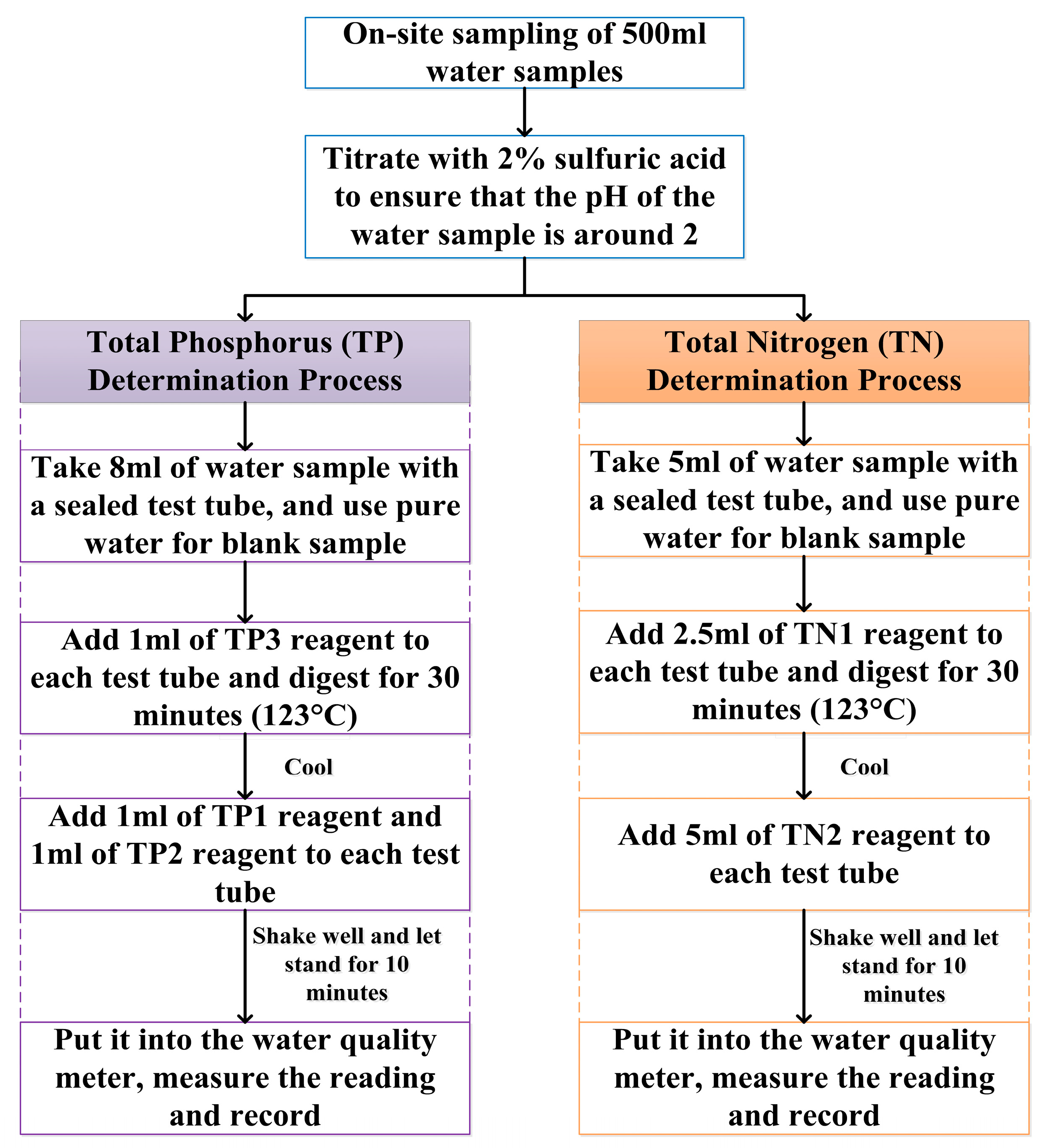
DO concentrations were measured on-site using an EXO2 multi-parameter water quality sonde manufactured by (YSI, Yellow Springs, OH, USA) [22]. TP and TN concentrations were determined from collected water samples using an SH-3900A multi-parameter water quality analyzer (SHINE, Shanghai, China) in conjunction with an SH-24 intelligent dual-temperature zone digestion instrument (SHINE, Shanghai, China). These two instruments must be used together during sampling and analysis. The detailed water quality measurement procedure is illustrated in Figure 3. In the figure, TP1, TP2, and TP3 correspond to the reagents LH-YGL, LH-YP1, and LH-YP2, respectively, while TN1 and TN2 correspond to the reagents NTA and NTB, respectively. All specific reagents were supplied by the instrument manufacturer.

2.2. Numerical Model Construction

2.2.1. Development of the MIKE Hydrodynamic—Water Quality Model

The core strength of the MIKE model lies in its efficient physics-based numerical solution and modular coupling design, enabling it to achieve both accuracy and flexibility in studies of water quality–hydrodynamic interactions. Its coupling mechanism quantitatively captures the synergistic effects of water environmental factors, providing a scientific basis for refined management and offering comprehensive solutions for complex hydraulic problems [23]. Consequently, this study utilized the hydrodynamic (HD) module and water quality (ECO Lab) module within MIKE 21 to simulate and analyze river water quality in the study area. The model’s predictive capability fundamentally resides in its advanced dynamic coupling framework as follows: the MIKE 21 HD module precisely simulates flow, water levels, and turbulent diffusion processes driven by tides, wind, etc., simultaneously providing a real-time physical background field for water quality variations; the ECO Lab water quality and ecological module operates using deep dynamic coupling with the hydrodynamic processes, driving the transport and transformation of pollutants. Based on the physical fields generated by the hydrodynamic module, the water quality module computes pollutant transport and transformation via advection–diffusion–reaction equations Equation (1) [24]:
t hc + x uhc + x v x c = x h D x c x + y h D y c y + S c + P c
where c denotes the concentration of water quality state variables, unit/milligram per liter (mg/L); u and v represent velocity components in the advection term, unit/meter per second (m/s); D x and D y denote diffusion coefficients; S c signifies source-sink terms; and P c represents the chemical reaction kinetics governing concentration dynamics.
Hydrodynamic conditions directly govern the rate at which pollutants are transported and the extent to which they are dispersed, and water quality parameters such as water temperature and dissolved oxygen may, in turn, exert feedback effects on water density—generating buoyancy effects and establishing a bidirectional coupling mechanism. This precise resolution of interconnected physical processes represents the distinctive capability of MIKE 21, setting it apart from purely data-driven models.
(1) River Network Generalization
a. River Network Mesh Preprocessing
This study employed the MIKE Flow Model to develop a hydrodynamic model, simulating river network flow dynamics based on an unstructured mesh. The river network within the study area was first delineated using the OMap (OMUAP) interactive map, with the computational domain defined by referencing 2022 Space View satellite imagery. To account for the Coriolis force effect, the projection system was set to WGS_1984_UTM_Zone_51N based on the geographical location of the study area. The delineated river network was then exported for mesh generation and processing within the MIKE ZERO mesh generator.
b. Mesh Generation and Sensitivity Control
Given the complex flow patterns in the plain river network, triangular unstructured mesh elements were adopted. To ensure simulation stability, land boundaries were smoothed and assigned uniformly distributed vertices. In response to significant variations in channel width, local refinement was implemented in narrower river sections. The maximum element area was controlled hierarchically according to channel width, ensuring adequate resolution in critical areas.
c. Mesh Quality Optimization
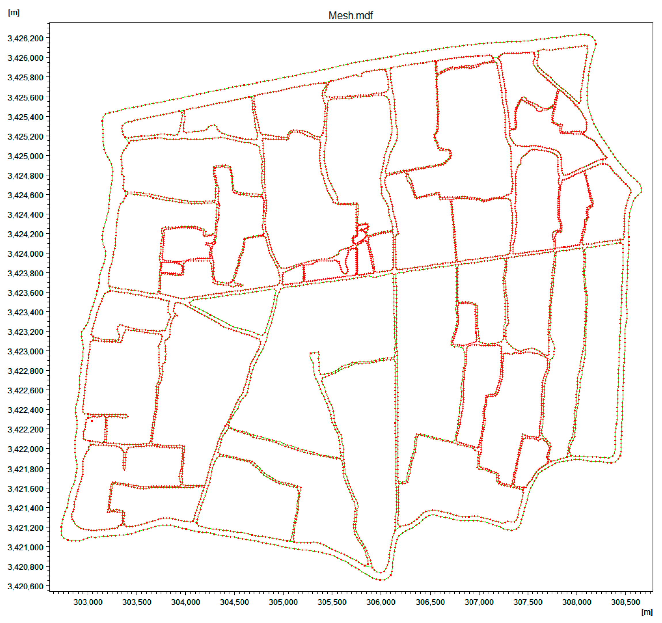
Following refinement, mesh quality was screened and optimized using the “Analyze mesh” tool. Elements exhibiting high skewness or minimum angles below 30 degrees were eliminated to ensure smooth mesh transitions and high overall quality. The final generated mesh consisted of 57,771 elements and 32,766 nodes, as shown in Figure 4, achieving a balance between accuracy and computational efficiency.
(2) Boundary Conditions
Setting boundaries is a critical step to ensure the correct flow direction and discharge configuration are used within the model [25]. In this study, open boundaries were defined primarily based on field hydrological surveys conducted at the Yaozhuang River in Jiashan during 2021–2022, regional water regulation records, and measured data from adjacent hydrological stations. Land boundaries were determined based on the Digital Elevation Model (DEM) and remote sensing imagery; the locations of open boundaries were identified by considering river confluence relationships, the distribution of sluices and dams, and the operational rules of hydraulic engineering structures. Flux boundaries were controlled by specifying inflows at upstream cross-sections, and water level boundaries were set using time-series data measured from a downstream tidal gauge station in order to accurately represent the input–output dynamics of regional water.
To determine the boundary configuration, we comprehensively considered the hydraulic characteristics of the plain river network and the availability of monitoring data. Both water level and discharge hydrographs were preliminarily compared against measured values to ensure that the simulated flow direction and dynamics aligned with reality. The model demonstrated reasonable water balance and flow response during subsequent calibration and validation, further indicating the reliability of the boundary settings. In summary, the established boundary conditions provided a solid foundation for realistic numerical simulations. This study established 10 open boundaries and 1 land boundary. The land boundary is uniformly designated as Code *, while the open boundaries are further grouped into inflow boundaries (Code2–Code6) designated as water-level boundaries and outflow boundaries (Code7–Code11) designated as discharge boundaries. The spatial configuration of these boundaries within the river network model is illustrated in Figure 5.
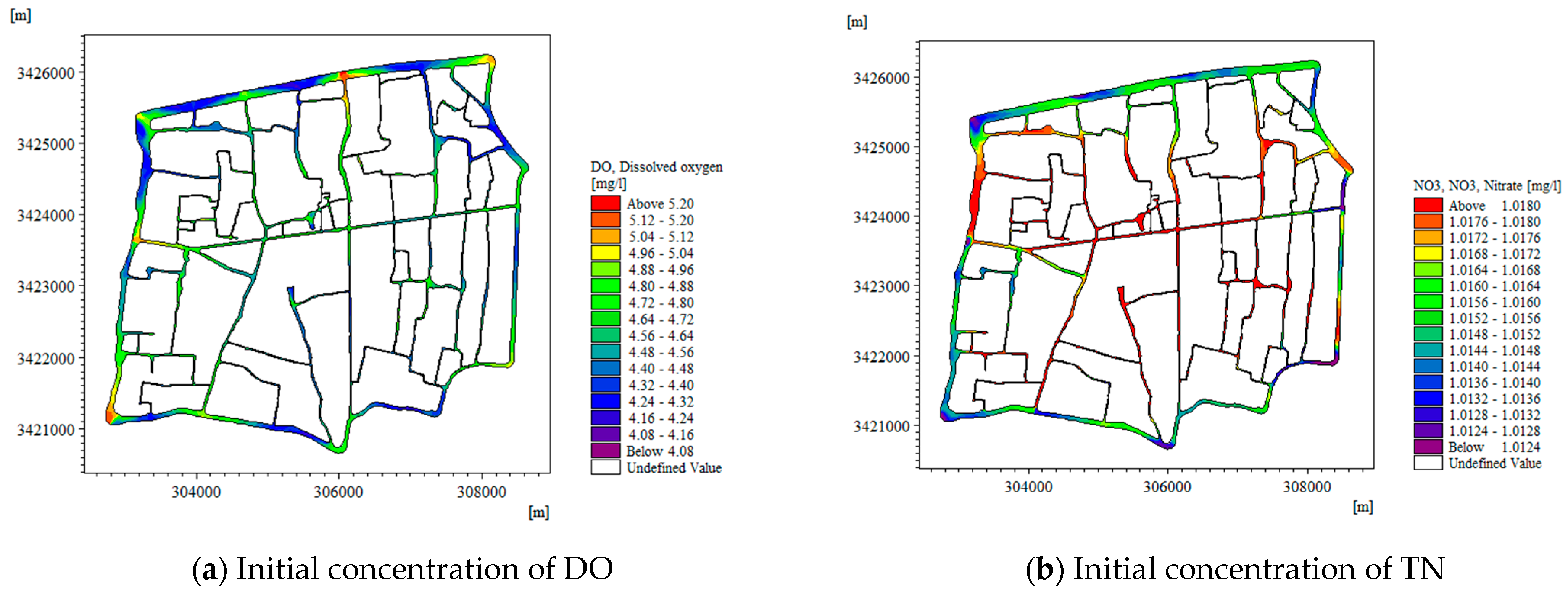
Boundary condition inputs for the water quality model comprised both constant water quality values and time-varying concentration sequences. To ensure the accuracy of simulations, this study utilized monthly water quality concentration measurements from 2022 to 2023—obtained from long-term monitoring datasets provided by the Jiashan Hydrological Bureau—as the boundary condition inputs. A hot start initialization method was implemented to achieve homogeneous distribution of water quality variables throughout the river network, thereby enhancing simulation precision. As shown in Figure 6, the initial post-hot start water quality concentrations across the river network exhibited high consistency with field measurements from monitoring stations upon comparative verification.
(3) Parameter Settings
The simulation utilized the “Mike Basin WQ model with oxygen” template from the water quality module. This WQ template is primarily designed for scenarios where anthropogenic pollution loads constitute the dominant source of contamination, and pollutants have a relatively short residence time in the water body. The Yaozhuang study area, located in the densely populated Jiashan County, features a river network where anthropogenic pollution is most prevalent, thus meeting the application criteria for the WQ template.
The “Mike Basin WQ model with oxygen” template incorporates seven predefined water quality state variables. The TN, TP, and DO parameters required for this simulation were configured directly within the template’s compiler.
In the actual simulation, pollutant loads entering the study area originated primarily from domestic, industrial, and agricultural sources. Furthermore, water quality parameter values varied across different regions and topographies. Incorrect parameter selection could severely compromise the accuracy of the simulation results. Therefore, the selection of water quality parameters involved an iterative process of adjustment, informed by a review of the relevant literature, to increase the agreement between simulated and measured values. This model comprehensively considered the current hydro-environmental conditions of the Yaozhuang river network as well as data from meteorological stations and the hydrological literature. An initial set of parameters was established based on analytical research, and values were subsequently refined through repeated calibration runs to determine the final, optimal parameter set for this specific regional model. Detailed information is provided in Table 2.

2.2.2. Development of the CNN-LSTM-Attention Model

The CNN-LSTM-Attention model developed in this study employs a three-tiered architecture to synergistically address inherent limitations of single-model approaches: the CNN layer [26,27,28] extracts spatial features from water quality parameters; the LSTM layer captures temporal dynamics as a specialized form of (RNN) [29]; and the Attention layer focuses on critical time periods. This integrated strategy resolves three major challenges in water quality simulation and prediction in plain river networks: (1). CNN-LSTM coupling enables spatiotemporal modeling, compensating for dimensional deficiencies in singular models; (2). the Attention mechanism mitigates lags in prediction in LSTM while enhancing sudden event detection; (3). Attention-driven weight pruning reduces computational redundancy in LSTM operations, thereby improving computational efficiency.
In this study, systematic parameter tuning was performed to optimize the key hyperparameters of the model, including the number and size of convolutional kernels in the CNN, the number of hidden units and dropout rate in the LSTM, and the dimension of the Attention mechanism. For instance, a large number of convolutional kernels allows the model to capture more diverse feature patterns, but it also increases computational cost, which may lead to overfitting. Therefore, each network layer of the CNN-LSTM-Attention model was precisely configured to fully adapt to the specific requirements of the water quality prediction task for the plain river network. The results, presented in Table 3, demonstrate that this configuration significantly enhanced the model’s ability to represent complex nonlinear relationships within the aquatic environment. The superiority of this method is evident in its lowest average RMSE across cross-validation folds and its parsimonious design, achieving an optimal balance between high accuracy, a lower risk of overfitting, and computational cost.
When evaluating the merits of a predictive model, it is generally necessary to employ a comprehensive set of evaluation metrics to assess its performance holistically. This study utilized three metrics: (1). Root Mean Square Error (RMSE), which quantifies the absolute deviation between predicted and measured values, shares units with the original data [30], and facilitates the intuitive interpretation of magnitudes of error; (2). Coefficient of Determination (R2), measuring the model’s explanatory capacity for data variability, where values closer to 1 indicate superior simulation performance; (3). Residual Prediction Deviation (RPD), which is an indicator of prediction accuracy [31], effectively evaluates the model’s precision and stability. Collectively, these metrics comprehensively evaluate model performance across three dimensions: error magnitude, goodness-of-fit, and model robustness.
To evaluate the predictive superiority of the model, the computational formulas for each metric are defined as follows:
M S E = 1 n i = 1 n y i y i 2
R M S E = M S E
R 2 = 1 i = 1 n y i y i 2 i = 1 n y i y ¯ 2
R P D = i = 1 n Residual i n
where n denotes sample size; y i represents the true value of the i-th sample; y i denotes the predicted value of the i-th sample; y ¯ signifies the mean of the dependent variable; and Residual indicates the residual deviation (actual prediction discrepancy).

2.3. Model Validation and Results Analysis

2.3.1. MIKE Model Validation Results

(1) Hydrodynamic Model Calibration and Validation
The hydrodynamic model in this study was calibrated using measured water level data from meteorological stations in 2022. Validation was conducted using monitoring points NO. 13, which is strategically located at the center of the river network to represent overall flow dynamics, along with NO. 4 and NO. 8. A comparison between simulated and measured water levels at these points is presented in Figure 7, while Figure 8 shows the corresponding absolute error percentages.
As shown in Figure 7 and Figure 8, the mean errors between the simulated and measured water levels at monitoring points NO. 13, NO. 4, and NO. 8 in the Yao River network in 2022 are 2.56%, 2.59%, and 2.42%, respectively. Overall, the simulation results show good agreement with the measured data, indicating that the established hydrodynamic model can effectively represent the flow field characteristics of the Yao River network and thus meets the requirements for simulation.
(2) Water Quality Model Calibration and Validation
Due to the irregular temporal resolution in water quality sampling within the study area, model validation employed monthly data measured from the Yaozhuang river network spanning 2022–2023. During validation, daily simulated water quality outputs were aggregated into monthly averages by calculating the arithmetic mean of all daily values within each month. This aggregation method aligns with the temporal resolution of the monitoring data and mitigates short-term fluctuations.
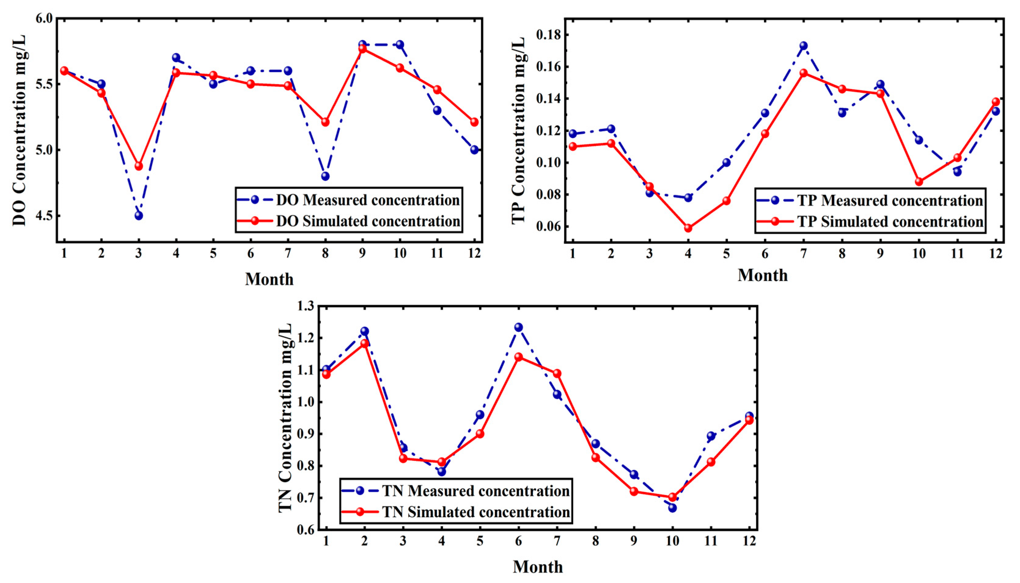
The hydrological conditions during 2022 and 2023 were incorporated into the model through time-varying boundary conditions based on monthly water quality concentration measurements from both years. Although interannual hydrological variability may influence pollutant loads (e.g., TN and TP), the use of monthly boundary conditions ensures that the model captures seasonal and annual differences in hydrodynamic and water quality processes. The consistent agreement between simulated and observed values (as shown in Figure 9) supports the robustness of this approach despite potential hydrological disparities.
Figure 9 reveals pronounced seasonal variations in water quality across the study area: the poorest conditions occurred from December to February, primarily attributed to suppressed microbial activity under low temperatures, prolonged hydraulic retention times, and reduced pollutant degradation rates; conversely, optimal water quality prevails from June to September, where elevated temperatures and increased rainfall synergistically enhance the self-purification capacity and pollutant transformation efficiency of water. Overall, the simulated concentrations exhibit close agreement with the measured values, demonstrating consistency with the spatiotemporal evolution patterns of river network water quality.
Table 4 presents the performance evaluation of water quality simulations. The results show simulated mean errors of 4–8% for DO, TN, and TP in the Yaozhuang river network. According to industry standards [32], error rates within 5–15% are acceptable for process-based commercial models. The R2 values for DO, TN, and TP are 0.889, 0.942, and 0.880, respectively, all exceeding the 0.8 benchmark and demonstrating robust goodness-of-fit. These outcomes confirm the high reliability of the model in simulating variations in spatiotemporal dynamics and water quality parameters across the study area.

2.3.2. CNN-LSTM-Attention Model Validation Results

This study utilized 4400 water quality samples from long-term monitoring data (January 2022 to February 2024) at the Hongqitang Dam station. The data underwent normalization preprocessing to eliminate dimensional effects and was divided at an 8:2 ratio: the training set (3520 samples) comprised the CNN-LSTM-Attention hybrid model, while the test set (880 samples) evaluated model generalization capability. During model training, MATLAB R2023a continuously monitored convergence of the loss function to ensure parameter optimization and network architecture stability.
(1) Calibration Results of Three Water Quality Parameters
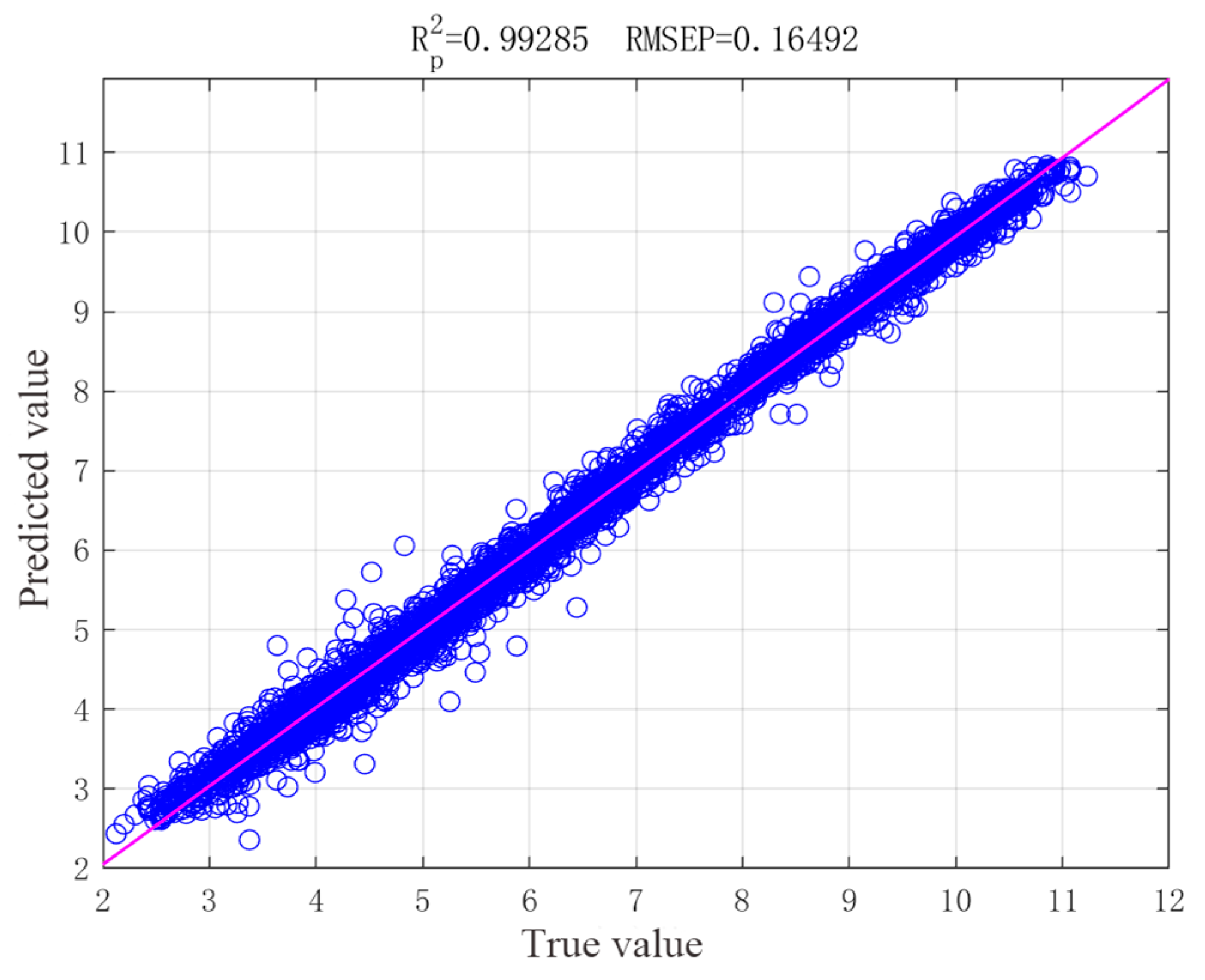
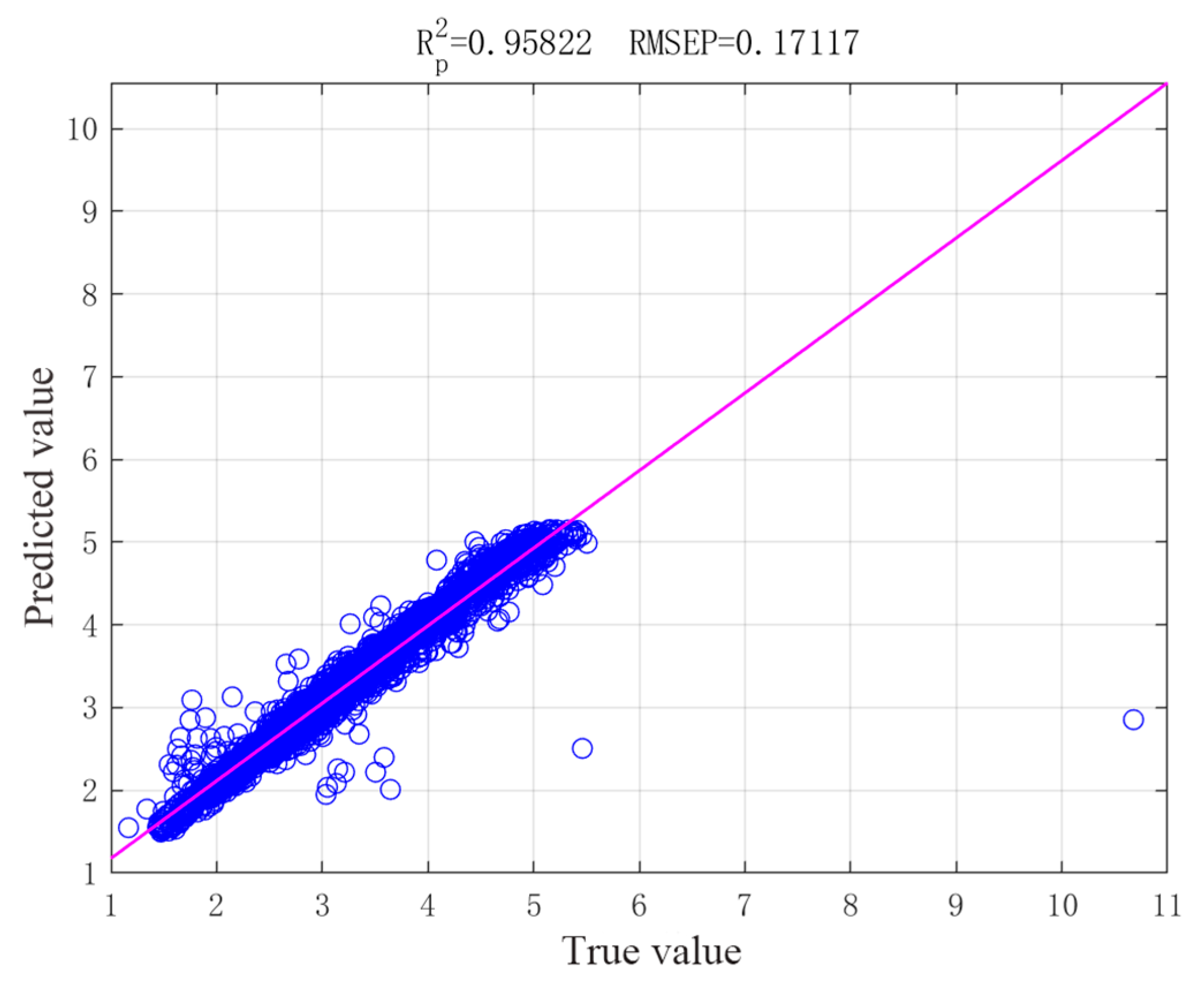
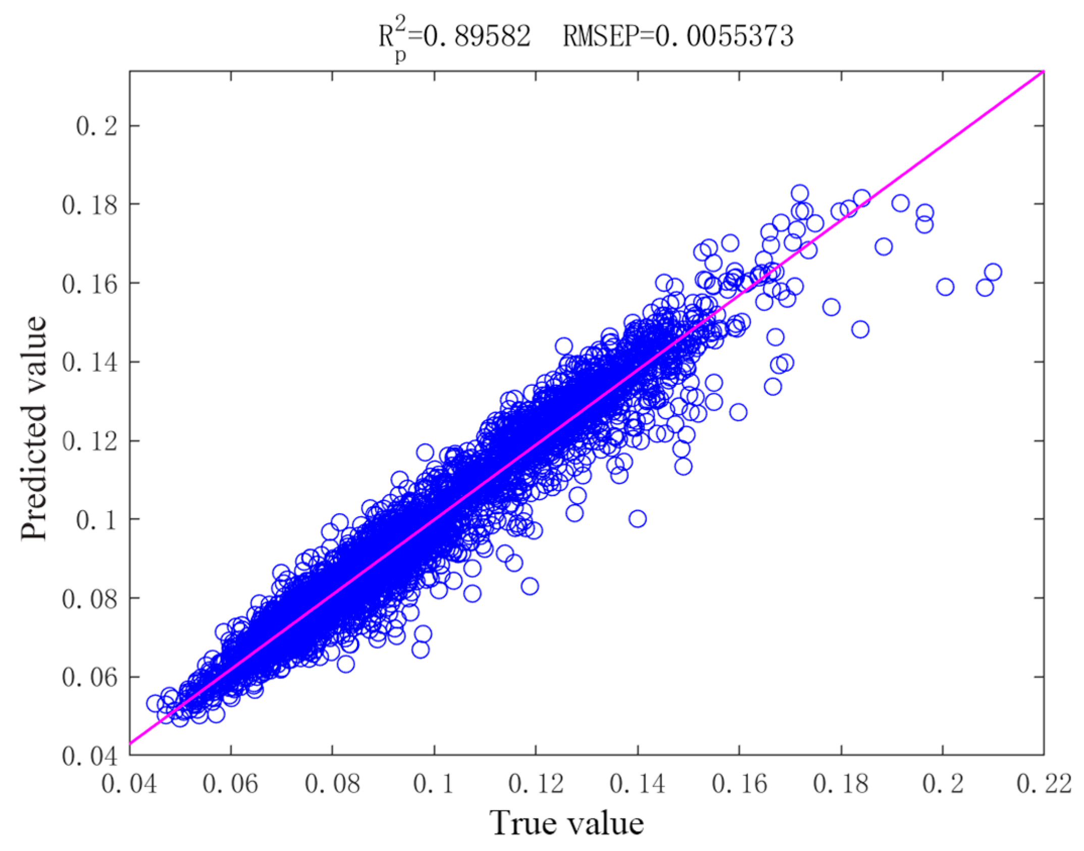
Fitting and prediction were performed for all samples of DO, TN, and TP. “Fitting” refers to the process by which the model learns the inherent patterns, relationships, and characteristics within the training data. “Prediction” refers to the already trained (fitted) model, which is used to infer outcomes for unknown data. The results are shown in Figure 10, Figure 11 and Figure 12.
The figures demonstrate that the established model exhibits excellent performance and fits well with the sample data. For dissolved oxygen (DO) samples, the model achieves high fitting precision with an R2 of 0.9929. Total nitrogen (TN) predictions also show relatively strong overall alignment (R2 = 0.9582); however, the scatter plot reveals several outlier points. In contrast, total phosphorus (TP) sample predictions display comparatively weaker performance (R2 = 0.8958); the model generated accurate predictions during the initial stage but showed increasingly dispersed and suboptimal results in later phases.
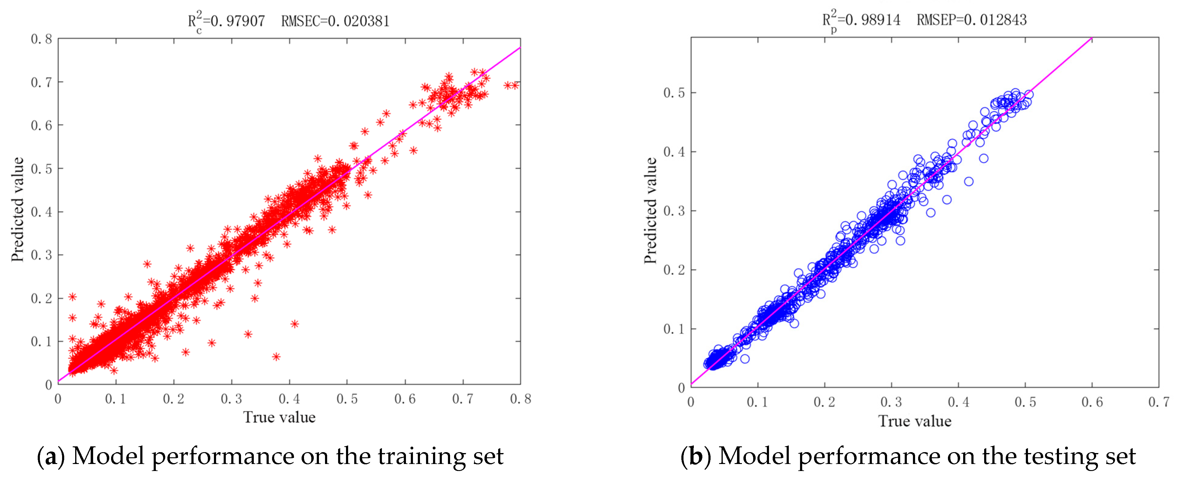
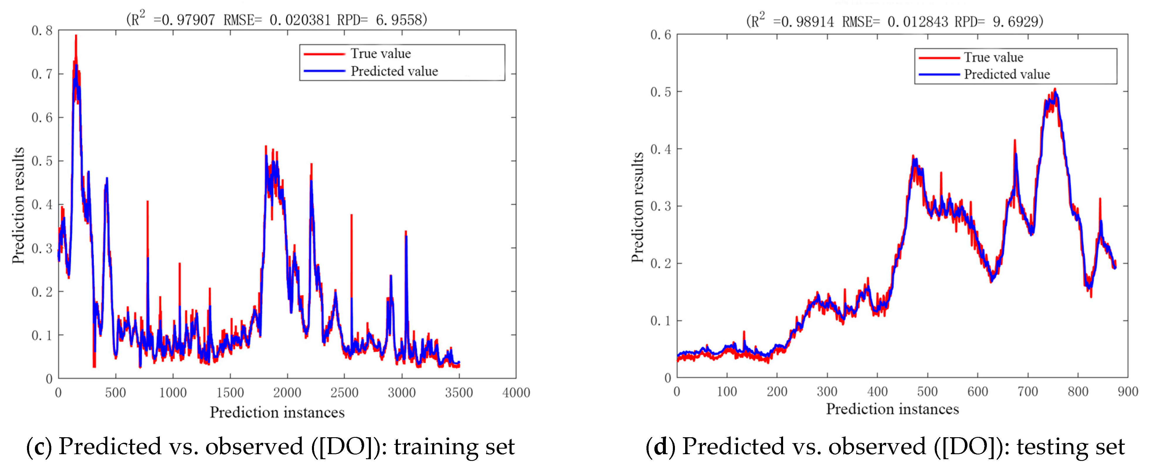
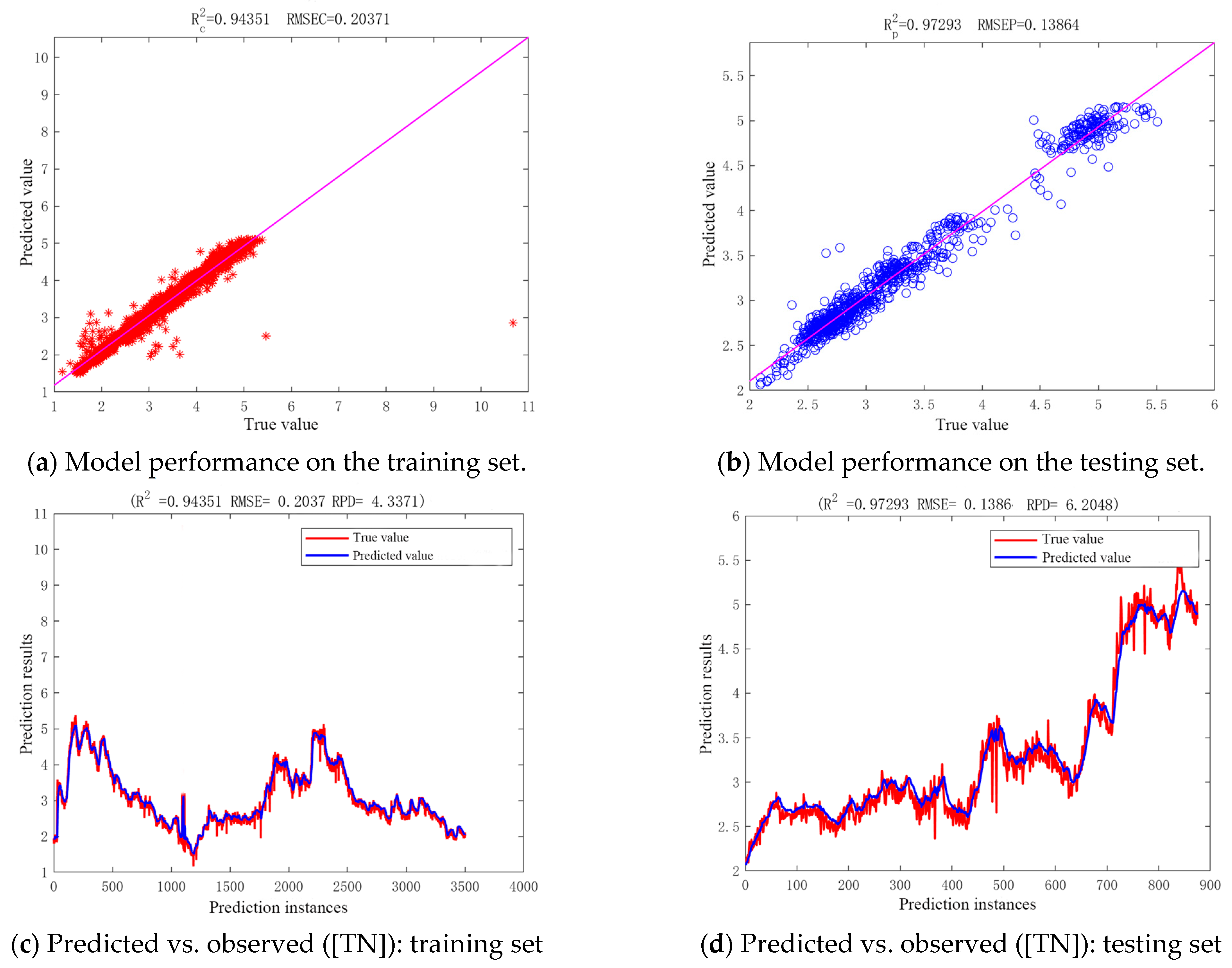
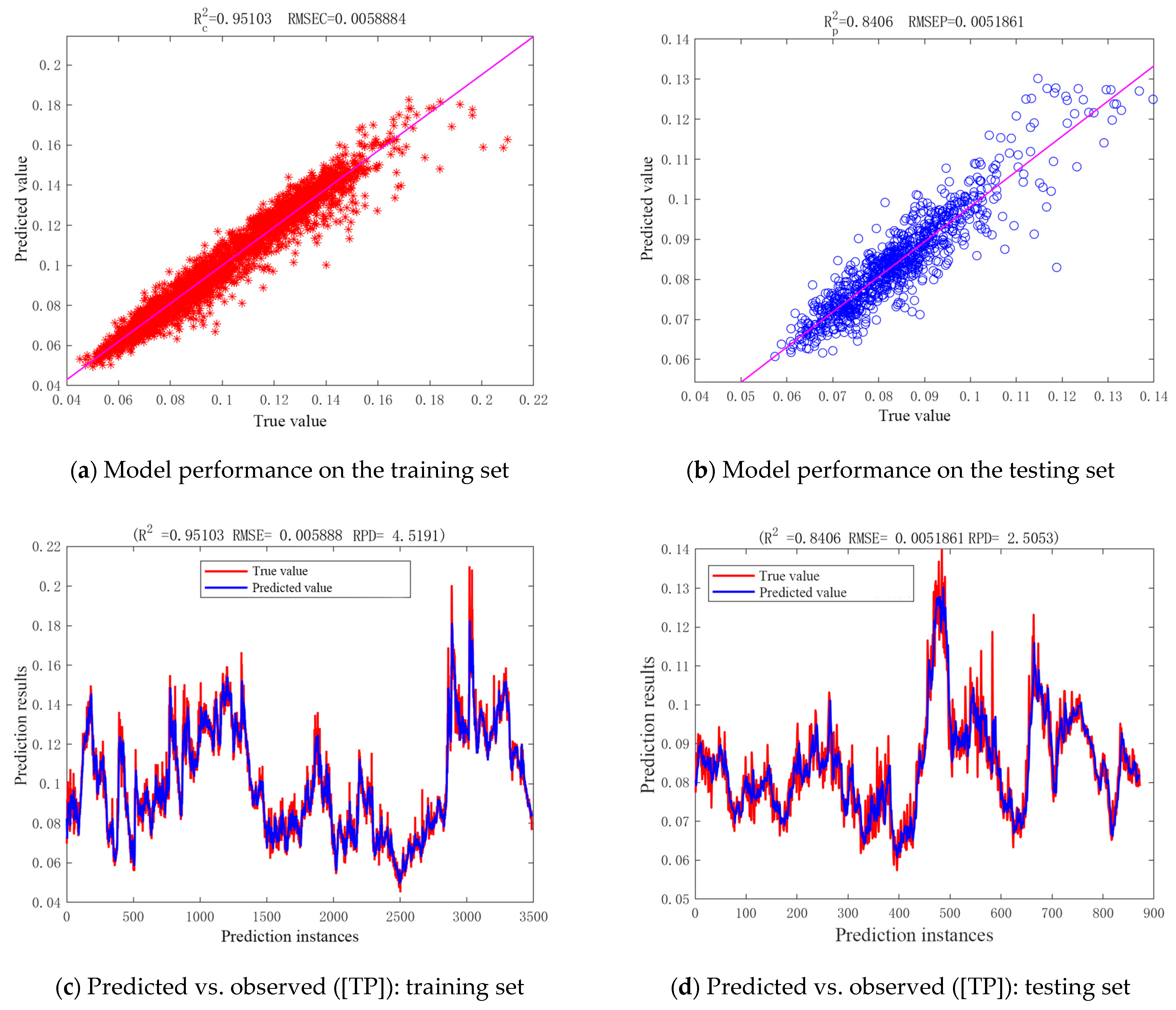
Figure 13, Figure 14, Figure 15 present comparative analyses of performance and prediction outcomes between the training and test sets for dissolved oxygen (DO), total nitrogen (TN), and total phosphorus (TP), respectively.
Figure 13a,c demonstrate excellent model performance for the training set, indicating that it effectively captured variations in measured dissolved oxygen (DO) concentrations with an R2 of 0.9923. Conversely, Figure 13b,d indicate superior test set performance (R2 = 0.9934), though deviations between simulated and observed values occurred during peak and trough segments. This reveals predictive limitations in abrupt DO transition zones.
As observed in Figure 14a,b, the model’s predictive performance on the test set surpassed its performance on the training set, demonstrating its exceptional generalization capability and accurate prediction of unseen data. This indicates that the learning process was effectively constrained by regularization, mitigating overfitting. Furthermore, Figure 14c,d corroborate that the training and test sets exhibit strong distributional consistency.
Figure 15a,b reveal a significant performance gap between training and test set predictions: the training set achieved an R2 of 0.95103, while the test set attained an R2 of 0.8406. The test set samples exhibited a widespread distribution, with higher prediction accuracy observed for values within the 0.06–0.1 range and a notably poorer performance for the 0.1–0.14 interval. Figure 15c,d further demonstrate that training set predictions showed minimal fluctuations with high fitting precision, whereas test set predictions displayed conservative behavior, overestimating lower true values and underestimating higher true values.
(2) Comparison of Prediction Model Performance
Table 5 compares the performance metrics of three prediction models: CNN, LSTM, and CNN-LSTM-Attention. Among these, the CNN-LSTM-Attention model achieved an R2 closest to 1, the lowest RMSE, and the highest RPD value, demonstrating superior prediction reliability. Consequently, the enhanced CNN-LSTM-Attention model exhibited optimal performance for predicting water quality indicators with high applicability when evaluated holistically.

3. Discussion

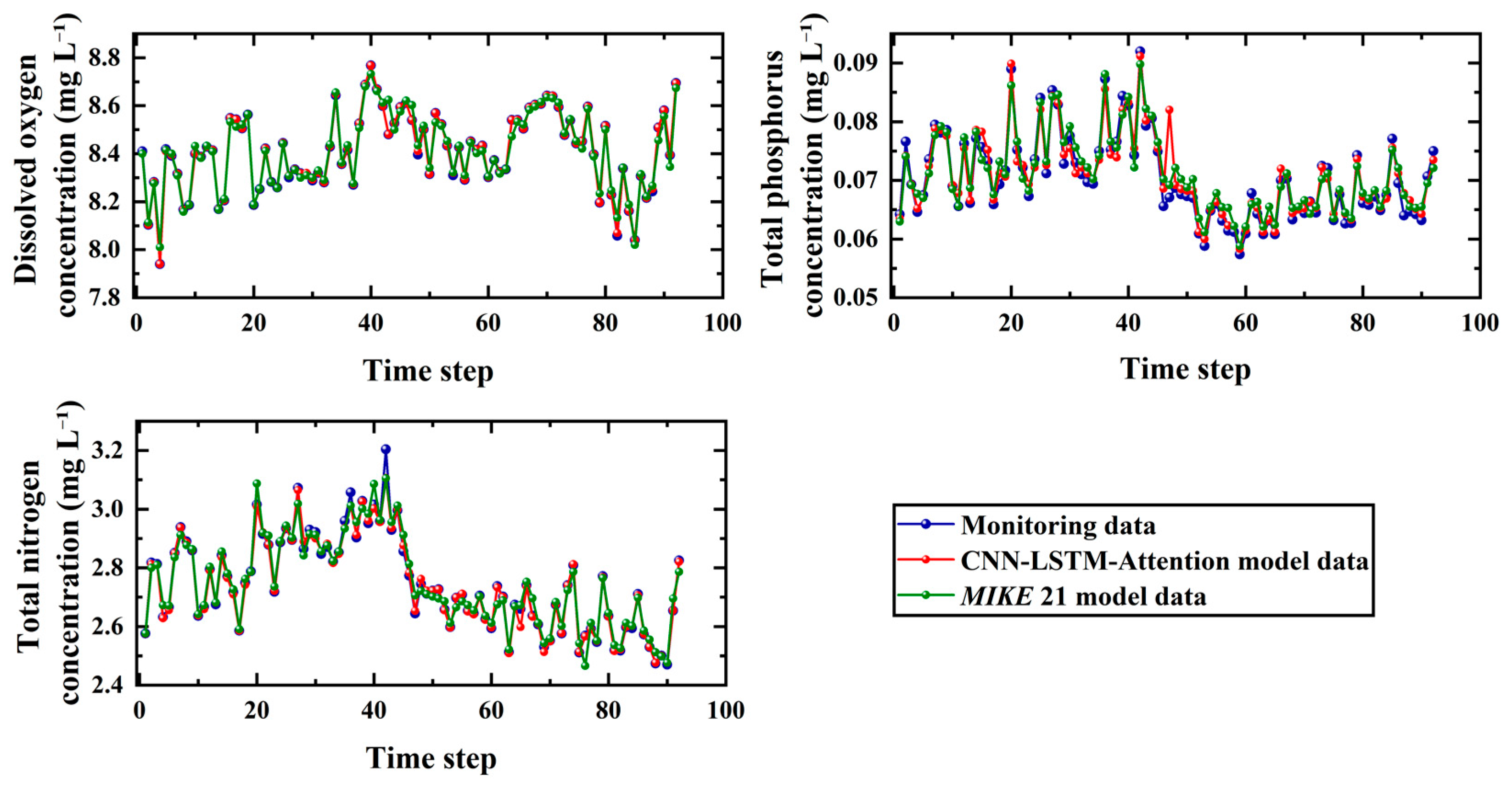
To investigate the differences in predictive accuracy and applicable scope between the MIKE 21 model and the CNN-LSTM-Attention model, this simulation utilized long-term time-series data from three water quality indicators released by the Hongqitang Dam monitoring station. Both models were employed to simulate daily water quality variations within the study area over a 92-day period from October to December 2023. A comparison with actual monitoring data (Figure 16) and a quantitative evaluation (Table 6) revealed that although both models demonstrate satisfactory predictive capability, they exhibit significant differences in their accuracy and scope of application.
Both models demonstrated strong statistical consistency with actual monitoring data in water quality prediction for the Yaozhuang river network; however, systematic differences in predictive accuracy were observed. The CNN-LSTM-Attention model achieved R2 values of 0.977 for DO and 0.982 for TN, significantly outperforming the MIKE 21 model (DO: 0.912, TN: 0.921). This hybrid model enhances the capability to resolve high-frequency fluctuations by extracting spatial features through convolutional layers, modeling long-term dependencies via LSTM, and reinforcing the weighting of critical time steps using an attention mechanism. Nevertheless, the model exhibited lower predictive accuracy for TP (R2 = 0.834) compared to the MIKE 21 model (R2 = 0.877). This discrepancy may stem from the fact that TP variation involves complex biogeochemical processes such as sediment-water interface exchange and algal uptake-release, whose response mechanisms are highly nonlinear and lagged. In this context, as noted by Bushra Tasnim et al. [33] in their comparison of one-dimensional and three-dimensional models, mechanistic frameworks such as EFDC+ demonstrate inherent advantages when addressing such well-defined processes, owing to their ability to directly describe and capture the spatial variability of physical and biochemical dynamics in water bodies.
In contrast, the MIKE 21 model demonstrated consistent stability across all three indicators (R2 > 0.87), highlighting its advantage in system-scale simulation, particularly in effectively quantifying the impact of key physical processes such as sluice gate operations on pollutant transport. This finding aligns with the view expressed by Quaghebeur Ward et al. [34] regarding the fundamental role of mechanistic models in representing well-defined physical processes. The application value and contemporary relevance of the MIKE 21 platform, as employed in this study, continue to be validated in international cutting-edge research. For instance, a recent study by Boris V. Divinsky et al. [35] utilized the MIKE 21 SW model to conduct a 45-year high-resolution climate simulation analysis of wind waves in the Black Sea, demonstrating the model’s capability and transferability in addressing complex environmental issues. However, its grid discretization approach and numerical solution procedures constrain its ability to resolve localized high-frequency dynamics, resulting in relatively lower accuracy in short-term, single-point predictions.
This study also identified inherent limitations associated with both model types. While the MIKE 21 model offers clear mechanistic interpretability, its construction and calibration rely heavily on extensive hydrological, topographic, and water quality parameters, limiting its applicability in data-scarce regions. Furthermore, its high computational cost hinders its use in real-time prediction applications. In contrast, although the CNN-LSTM-Attention model possesses efficient nonlinear fitting capability and potential for real-time forecasting, its performance is heavily dependent on the quality and volume of training data. The model training in this study utilized 21 months of high-frequency monitoring data from January 2022 to September 2023; however, issues with data gaps remained, and the model exhibited higher uncertainty in predicting extreme hydrological events (such as storm rainfall and severe droughts), indicating that its generalization capability requires further improvement. This finding aligns with the recent observation by Sanika Baste et al. [36] regarding the instability of data-driven models under extrapolation conditions.
Based on the findings above, this study concludes that model selection should be closely aligned with specific application scenarios. The CNN-LSTM-Attention model demonstrates superior performance for short-term real-time warning or point predictions where data are abundant, whereas the MIKE 21 model proves more suitable for scenarios requiring the identification of pollution sources, assessment of engineering intervention effects, or simulation of complex hydrodynamic-water quality coupling processes.
In summary, purely mechanistic or data-driven models each possess inherent limitations. Future research should explore integrated approaches that embed physical mechanisms within data-driven frameworks. As Sheikholeslami et al. [37] envisioned, developing physics-informed machine learning models represents a critical pathway toward enhancing model extrapolation capability and interpretability. Furthermore, the hybrid modeling strategy advocated by Quaghebeur et al. [34]—which integrates physical mechanisms with data-driven methods—is recognized as a promising solution that balances mechanistic rigor with powerful fitting capacity for complex nonlinear relationships. This trend has been widely evidenced in international research: a representative example includes the work by Kim, S. et al. [38] in South Korea, who integrated convolutional neural networks (CNN) with the physical hydrological model (HGS) in the Sabgyo River Basin. This achieved high-resolution spatiotemporal estimation of groundwater head and surface water depth, improving computational speed by 45 times compared to a purely mechanistic model while effectively combining the advantages of both physical mechanisms and data-driven approaches. Similarly, Zhong, M. et al. [39] developed two hybrid models, VIC-CaMa-Flood-RNN (VCR) and VIC-CaMa-Flood-LSTM (VCL), which incorporate both physics-based and data-driven components, further enhancing the accuracy of streamflow and flood predictions and providing reliable support for future flood risk assessment. Erge Oney et al. [40] proposed a hybrid modeling method combining physics-based and data-driven models for predicting drilling riser pressure, effectively circumventing certain limitations inherent in purely physical or purely data-driven models. Therefore, the findings and methodology presented in this study establish a solid foundation for developing advanced hybrid models in this field. Future research could explore deeply coupling the established MIKE 21 mechanistic model as a physical kernel with data-driven methods such as CNN-LSTM-Attention. This direction not only aligns with international frontiers but also, through its successful implementation, demonstrates the strong transferability of the approach. It holds promise for providing accurate, efficient, and reliable simulation and prediction tools for other water bodies facing similarly complex hydro-environmental conditions.

4. Conclusions

(1)
The physics-based MIKE 21 model excels in simulating spatiotemporal distributions of hydrodynamics and water quality parameters across the river network (R2 > 0.88 for all three indicators), quantitatively capturing the impacts of sluice gates and the causal relationships between hydrodynamics and water quality. Its strengths in spatial resolution and physical interpretability cannot be replicated by deep learning approaches.
(2)
The CNN-LSTM-Attention model integrates spatial feature extraction and temporal modeling, and focuses on critical events, significantly enhancing point-scale prediction accuracy (DO R2 = 0.9934; TN R2 = 0.9435) for complex nonlinear dynamics and high-frequency fluctuations. However, its lower TP prediction accuracy (R2 = 0.8406) indicates limitations in simulating processes involving interfacial exchanges and complex biochemical reactions like phosphorus cycling.
(3)
Practical applications require model–target alignment: the CNN-LSTM-Attention is preferred for high-precision short-term forecasting or real-time alerts with sufficient data, while MIKE 21 is better suited for identifying the spatial mechanisms of pollutants, evaluating engineering measures, or simulating complex hydrological scenarios.
(4)
Future work should develop physics-informed hybrid models by integrating MIKE 21’s hydrodynamic fields as feature inputs and enhancing reliability through physical constraints to synergize both paradigms, ultimately strengthening the precision management of river network water environments.

Author Contributions

Conceptualization, Y.L., C.X. and L.D.; Methodology, Y.L., C.X. and L.D.; Software, Y.L., M.W. and Z.R.; Validation, Y.L. and Z.R.; Formal analysis, Y.L.; Investigation, Z.R. and Z.W.; Data curation, Y.L. and Z.W.; Writing—original draft, Y.L.; Writing —review & editing, Y.L., C.X. and M.W.; Visualization, Y.L.; Supervision, C.X., L.D. and M.W.; Project administration, C.X. All authors have read and agreed to the published version of the manuscript.

Funding

This research was funded by the Basic Public Welfare Research Program of Zhejiang Province (LZJWD22E090001) and the Major Science and Technology Program of Zhejiang Province (2021C03019).

Data Availability Statement

The datasets presented in this article are not readily available because they constitute key supporting material for subsequent patent applications and commercial development, and are therefore not publicly accessible at this stage. Requests to access the datasets should be directed to 15869219184@163.com.

Conflicts of Interest

The authors declare no conflict of interest.

References

  1. Xu, T.Y.; Liu, K.Q.; Shan, Y.S.; He, S. Flood control situation analysis and countermeasure research for river network areas in the Hangjiahu Plain. China Rural Water Hydropower 2019, 2019, 123–125. [Google Scholar]
  2. Zou, S.W.; Wang, H.Z.; Yuan, S.J. Key technologies and case analysis for water quality enhancement in plain river networks: A case study of Hongkou waterways. Water Purif. Technol. 2022, 41, 116–121. [Google Scholar]
  3. Li, X.; Tang, H.W.; Wang, L.L.; Hu, Z.J.; Jiao, C. Hydro-environmental simulation of integrated regulation of sluice-pump systems in plain river network regions. J. Hohai Univ. (Nat. Sci.) 2016, 44, 393–399. [Google Scholar]
  4. Huang, Z.R.; Miao, Y.; Zhang, Z.L. Development of flood control decision support system for plain river network cities in Taihu Basin. People's Yangtze 2023, 54, 16–19. [Google Scholar]
  5. Xu, C.D.; Zi, Y.H.; Huang, S.; Zhao, Z.H.; Ren, Z.H.; Hu, X.M.; Wang, H.R. Hydrodynamic regulation method for polder river networks based on MIKE 21. Water Resour. Hydropower Eng. 2023, 54, 161–170. [Google Scholar]
  6. Zainescu, F.; Vespremeanu-Stroe, A.; Anthony, E.; Tatui, F.; Preoteasa, L.; Mateescu, R. Flood deposition and storm removal of sediments in front of a deltaic wave-influenced river mouth. Mar. Geol. 2019, 417, 106015. [Google Scholar] [CrossRef]
  7. Khatib, M.; Kahil, M.; Soliman, M.R. Restoration of Qaraoun Lake aquatic life based on wetland treatment concept. Heliyon 2023, 9, e18169. [Google Scholar] [CrossRef]
  8. Ahmed, A.; Aidi, H.; Liu, Q.; Zhao, X.T.; Zhao, S.M. Tracing heavy metal migration in stone coal mining watersheds: Insights from coupled SWAT-MIKE21-ECO lab simulations. Chemosphere 2025, 385, 144588. [Google Scholar] [CrossRef]
  9. Elshemy, M.; Khadr, M.; Atta, Y.; Ahmed, A. Hydrodynamic and water quality modeling of Lake Manzala (Egypt) under data scarcity. Environ. Earth Sci. 2016, 75, 1329. [Google Scholar] [CrossRef]
  10. Hosseini-Sadabadi, S.A.; Rousseau, N.A.; Laurion, I.; Behmel, S.; Sadeghian, A.; Foulon, E.; Wauthy, M.; Cantin, A.-M. Spatiotemporal insights of phytoplankton dynamics in a northern, rural-urban lake using a 3D water quality model. J. Environ. Manag. 2024, 370, 122687. [Google Scholar] [CrossRef]
  11. Al-Rikab, W.J.; Abed Basim, S. Hydraulic behaviour and improving of water quality of the Chibayish Marshes. Mater. Today Proc. 2022, 60, 1459–1467. [Google Scholar] [CrossRef]
  12. Qin, Z.; He, Z.; Wu, G.; Tang, G.; Wang, Q. Developing Water-Quality Model for Jingpo Lake Based on EFDC. Water 2022, 14, 2596. [Google Scholar] [CrossRef]
  13. Maruthamuthu, R.; Balamurugan, S.; Kumar, N.N.; Kumar, K.D. Enhanced Water Quality Index Prediction using a Dual-Key Convolutional Transformer Autoencoder Network Integrating with Poplar Optimization. Franklin Open 2025, 100370. [Google Scholar] [CrossRef]
  14. Wai, K.P.; Koo, C.H.; Huang, Y.F.; Chong, W.C.; El-Shafie, A.; Sherif, M.; Ahmed, A.N. A practical temporal transfer learning model for multi-step water quality index forecasting using A CNN-coupled dual-path LSTM network. J. Hydrol. Reg. Stud. 2025, 60, 102553. [Google Scholar] [CrossRef]
  15. Meysam, A.; Salim, H.; Sungwon, K. A robust and explainable deep learning model based on an LSTM-CNN framework for reliable FDOM prediction in water quality monitoring: Incorporating SHAP analysis for enhanced interpretability. Process Saf. Environ. Prot. 2025, 107594. [Google Scholar] [CrossRef]
  16. Wang, Y.F.; Xie, L.Z.; Zhang, J.J.; Tian, Y.Z.; Li, S.S.; Wang, Y.G. Performance Evaluation of Water Quality Prediction for Different Durations Based on the ED-LSTM Model. South-North Water Transf. Water Sci. Technol. (Chin. Engl.), 2025; in press. [Google Scholar]
  17. Liu, K.; Liu, F.; Peng, Y.X.; Zhang, S.N.; Fan, J.; Du, X.N.; Wang, Z.R. Evaluation and Prediction of Watershed Water Quality Based on Machine Learning Models. Environ. Pollut. Control 2025, 47, 1–10. [Google Scholar]
  18. Xiao, F.; Zhang, R.; Jian, Z.; Liu, W.; Sun, T.; Pang, W.; Han, L.; Qin, H. Using ensemble machine learning to predict and understand spatiotemporal water quality variations across diverse watersheds in coastal urbanized areas. Ecol. Indic. 2025, 178, 113976. [Google Scholar] [CrossRef]
  19. Melikoglu, M. Predictive hybrid modelling for municipal water and wastewater: A global framework demonstrated in Türkiye. Cleaner Water 2025, 4, 100117. [Google Scholar] [CrossRef]
  20. GB 3838-2002; Environmental Quality Standards for Surface Water. Ministry of Environmental Protection of the People’s Republic of China: Beijing, China, 2002.
  21. Zhao, Y.H. Economic benefit analysis of flood control projects in polder areas: Case study of Yaozhuang Polder in Jiashan County. Zhejiang Hydrotech. 2010, 38–42. [Google Scholar] [CrossRef]
  22. Li, W.X.; Jiang, M.L.; Xu, L.G.; Hu, S.P.; You, H.L.; Zhou, Q.P.; Chen, Z.; Zhang, L. Spatiotemporal variation of phytoplankton in Poyang Lake and its response to extreme flood and drought events. J. Lake Sci. 2024, 1–15. [Google Scholar]
  23. Ju, J.Y.; Liu, J.G.; Zhang, X.L.; Hu, D.D.; Li, Z.Y. Study on Urban Flood Simulation in Zhengdong New District Based on MIKE Coupled Model. Water Resour. Power 2025, 16–20. [Google Scholar]
  24. Suriya, S.; Mudgal, B.V. Impact of urbanization on flooding: The Thirusoolam sub watershed-A case study. J. Hydrol. 2012, 412–413, 210–219. [Google Scholar] [CrossRef]
  25. Wahyudi, W.; Martono, D.; Utomo, S.; Sutjiningsih, D. Investigating Impact of Sea Sand Mining in Tunda Island Waters, Indonesia Based in Mike 21 Modelling. Croat. J. Fish. 2023, 81, 73–81. [Google Scholar] [CrossRef]
  26. Quinteros-Cartaya, C.; Köhler, J.; Li, W.; Faber, J.; Srivastava, N. Exploring a CNN model for earthquake magnitude estimation using HR-GNSS data. J. South Am. Earth Sci. 2024, 136, 136104815. [Google Scholar] [CrossRef]
  27. Cheng, Y.; Yin, H.L. A water quality prediction model for municipal pumping stations based on feature extraction optimization and CNN-LSTM. Acta Sci. Circumstantiae 2025, 1–9. [Google Scholar] [CrossRef]
  28. Salem, M.S.; Hassan, N.M.H.; Aly, M.M.; Soliman, Y.; Peters, R.W.; Mostafa, M.K. Integrating Deep Learning and Process-Based Modeling for Water Quality Prediction in Canals: CNN-LSTM and QUAL2K Analysis of Ismailia Canal. Sustainability 2025, 17, 7743. [Google Scholar] [CrossRef]
  29. Hassan, N.; Miah, M.S.A.; Shin, J. A Deep Bidirectional LSTM Model Enhanced by Transfer-Learning-Based Feature Extraction for Dynamic Human Activity Recognition. Appl. Sci. 2024, 14, 603. [Google Scholar] [CrossRef]
  30. Jin, C.; Li, B.; Yang, L.F.; Zhou, X.Z. Open channel flow velocity prediction model based on machine learning-CFD. People's Yangtze 2023, 54, 166–174. [Google Scholar]
  31. Ren, P.; Chen, M.X.; Cao, W.H.; Wang, Z.; Han, L.; Song, L.; Yang, L. Error analysis and correction of short-term numerical weather prediction under complex terrain based on machine learning. Acta Meteorol. Sin. 2020, 78, 1002–1020. [Google Scholar]
  32. Li, W.L. Research on Sequence Recommendation Algorithm Integrating Attention Mechanism and Multimodal Information. Master’s Thesis, Tianjin University of Technology, Tianjin, China, 2023. [Google Scholar]
  33. Tasnim, B.; Fang, X.; Hayworth, J.S. Hayworth. One- and Three-Dimensional Hydrodynamic, Water Temperature, and Dissolved Oxygen Modeling Comparison. Water 2024, 16, 317. [Google Scholar] [CrossRef]
  34. Quaghebeur, W.; Torfs, E.; De Baets, B.; Nopens, I. Hybrid differential equations: Integrating mechanistic and data-driven techniques for modellingof water systems. Water Res. 2022, 213, 118166. [Google Scholar] [CrossRef]
  35. Boris, V.; Divinsky, Y.; Saprykina, V. Quasi-homogeneous regions of climatic distributions of wind wave parameters in the Black Sea. Dyn. Atmos. Ocean. 2025, 110, 101535. [Google Scholar] [CrossRef]
  36. Baste, S.; Klotz, D.; Acuña Espinoza, E.; Bardossy, A.; Loritz, R. Unveiling the Limits of Deep Learning Models in Hydrological Extrapolation Tasks. EGUsphere, 2025; preprint. [Google Scholar]
  37. Sheikholeslami, R.; Hall, J.W. Global patterns and key drivers of stream nitrogen concentration: A machine learning approach. Sci. Total Environ. 2023, 868, 161623. [Google Scholar] [CrossRef]
  38. Kim, S.; Lee, E.; Hwang, H.-T.; Pyo, J.; Yun, D.; Baek, S.-S.; Cho, K.H. Spatiotemporal estimation of groundwater and surface water conditions by integrating deep learning and physics-based watershed models. Water Res. 2024, 23, 100228. [Google Scholar] [CrossRef]
  39. Zhong, M.; Zhang, H.R.; Wang, Y.F.; Geng, H. Runoff prediction using a hybrid physical mechanism and deep learning approach. Yunnan Electr. Power Technol. 2023, 51, 2–6+12. [Google Scholar]
  40. Erge, O.; van Oort, E. Combining physics-based and data-driven modeling in well construction: Hybrid fluid dynamics modeling. J. Nat. Gas Sci. Eng. 2022, 97, 104348. [Google Scholar] [CrossRef]
Figure 1. Geographical location of Yaozhuang Weir area.
Water 17 02948 g001
Figure 2. Schematic map showing the geographic locations of monitoring points.
Water 17 02948 g002
Figure 3. Schematic diagram of water quality testing methods.
Water 17 02948 g003
Figure 4. Grid map of the river network model in the study area.
Water 17 02948 g004
Figure 5. Schematic diagram of boundary positions.
Water 17 02948 g005
Figure 6. Initial concentration conditions for the water quality model: (a) Dissolved Oxygen (DO); (b) Total Nitrogen (TN); (c) Total Phosphorus (TP).
Water 17 02948 g006aWater 17 02948 g006b
Figure 7. Comparison of simulated and measured water levels in the Yaozhuang river network: (a) Water Level: Simulated vs. Observed at Station No. 13. (b) Water Level: Simulated vs. Observed at Station No. 4. (c) Water Level: Simulated vs. Observed at Station No. 8.
Water 17 02948 g007
Figure 8. Graph of absolute error rates between simulated and measured water levels. (a) Absolute Error of Water Level at Station No. 13. (b) Absolute Error of Water Level at Station No. 4. (c) Absolute Error of Water Level at Station No. 8.
Water 17 02948 g008
Figure 9. Comparison of measured water quality values and simulated results for the Yaozhuang river network in 2022.
Water 17 02948 g009
Figure 10. DO sample fitting and prediction.
Water 17 02948 g010
Figure 11. TN sample fitting and prediction.
Water 17 02948 g011
Figure 12. TP sample fitting and prediction.
Water 17 02948 g012
Figure 13. Performance of the CNN-LSTM-Attention model for Dissolved Oxygen (DO) prediction. (a) Time-series comparison between predicted and observed DO concentrations on the training set; (b) Time-series comparison on the testing set; (c) Scatter plot of predicted vs. observed DO concentrations on the training set; (d) Scatter plot of predicted vs. observed DO concentrations on the testing set.
Water 17 02948 g013aWater 17 02948 g013b
Figure 14. Performance of the CNN-LSTM-Attention model for Total Nitrogen (TN) prediction. (a) Time-series comparison between predicted and observed TN concentrations on the training set; (b) Time-series comparison on the testing set; (c) Scatter plot of predicted vs. observed TN concentrations on the training set; (d) Scatter plot of predicted vs. observed TN concentrations on the testing set.
Water 17 02948 g014
Figure 15. Performance of the CNN-LSTM-Attention model for Total Phosphorus (TP) prediction. (a) Time-series comparison between predicted and observed TP concentrations on the training set; (b) Time-series comparison on the testing set; (c) Scatter plot of predicted vs. observed TP concentrations on the training set; (d) Scatter plot of predicted vs. observed TP concentrations on the testing set.
Water 17 02948 g015
Figure 16. Comparison chart of predictive model data.
Water 17 02948 g016
Table 1. Summary of data used in this study.
Data PurposeData SourceData TypeTime PeriodModel/Analysis Applied
Hydrodynamic model calibration and validationPolder Meteorological StationWater LevelYear 2022MIKE 21 HD Module
Water quality model calibration and validationJiashan Hydrological BureauMonthly Water Quality (DO, TN, TP)Year 2022–Year 2023MIKE 21 ECO Lab Module
Deep learning model training and testingHongqitang Dam Station Long-term MonitoringHigh-frequency Water Quality (DO, TN, TP)January 2022–February 2024CNN-LSTM-Attention Model
Comparative analysis of both modelsField Monitoring dataDaily Water Quality (DO, TN, TP)October–December 2023MIKE 21 and CNN-LSTM-Attention Models
Table 2. Values of water quality model parameters.
Parameter SymbolParameter DescriptionValueUnit
DOMaximum oxygen concentration at noon2per day
Half-saturation constant for respiration2mg/L
Plant respiration rate0.125per day
Respiration temperature coefficient1.08dimensionless
Oxygen demand for nitrification (NH4-NO2)3.44gO2/g NH3-N
Oxygen demand for nitrification (NO2-NO3)1.12gO2/g NO2-N
Half-saturation constant for sediment oxygen demand2mg/L
Sediment oxygen demand (per m2)0.5per day
SOD temperature coefficient1.05dimensionless
TPPhosphorus fraction in dissolved COD1.088--
Phosphorus uptake by plants0.092g P/g DO
Phosphorus uptake by bacteria0.015g P/g DO
Half-saturation constant for P uptake0.005mg/L
TNHalf-saturation constant for nitrogen uptake0.05mg/L
Nitrogen uptake by bacteria0.108g N/g DO
First-order decay rate for nitrification0.05per day
Half-saturation constant for oxygen in nitrification2mg/L
Note: For the model parameters not specified in the table, the default values from the ECOLAB template are adopted.
Table 3. Parameter settings for the CNN-LSTM-Attention model.
Layer TypeParameterSetting ValueDesign Purpose
CNNKernel Size(3, 3)Capturing local spatial features and patterns.
Number of Kernels64Extracting high-dimensional spatial representations.
Activation FunctionReLUIntroducing nonlinearity.
LSTMHidden Units128Modeling temporal dependencies and long-term dynamics.
Timesteps100Providing sufficient historical contexts for prediction.
Dropout Rate0.2Mitigating overfitting for better generalization.
AttentionAttention MechanismBahdanau AttentionFocusing adaptively on critical time steps for decoding.
Attention Dimensionality32Balancing representational capacity and computational cost.
OthersOptimizerAdamEfficient optimization of complex nonlinear models.
Learning Rate0.001Ensuring stable convergence.
Batch Size32Balancing training efficiency and gradient stability.
Epochs8100Sufficient for model convergence.
Loss FunctionCross-Entropy LossSuitable for classification tasks.
Table 4. Evaluation of the simulation effect of the water quality model.
Water Quality IndicatorsDOTNTP
R20.8890.9420.880
δ6.57%4.82%7.12%
Table 5. Comparison of evaluation metrics for prediction model.
Performance IndexFull Dataset (Training + Test)CNNLSTMCNN-LSTM-Attention
RMSEDO0.25320.22600.1649
TN0.34460.30260.1712
TP0.00770.00750.0055
R2DO0.91670.96130.9929
TN0.90920.92700.9582
TP0.84590.85740.8958
RPDDO7.76198.559512.0074
TN3.58133.85015.2709
TP2.49022.61473.5122
Table 6. Evaluation table for R2 of two prediction model indicators.
Prediction ModelDOTNTP
MIKE 21 Model0.9120.9210.877
CNN-LSTM-Attention Model0.9770.9820.834
Disclaimer/Publisher’s Note: The statements, opinions and data contained in all publications are solely those of the individual author(s) and contributor(s) and not of MDPI and/or the editor(s). MDPI and/or the editor(s) disclaim responsibility for any injury to people or property resulting from any ideas, methods, instructions or products referred to in the content.