Article

Past and Future Storm-Driven Changes to a Dynamic Sandy Barrier System: Outer Cape Cod, Massachusetts

1
Graduate School of Oceanography, University of Rhode Island, 215 South Ferry Rd., Narragansett, RI 02882, USA
2
Department of Ocean Engineering, University of Rhode Island, 15 Receiving Rd., Narragansett, RI 02881, USA
3
Environmental Data Center, University of Rhode Island, 1 Greenhouse Rd., Kingston, RI 02881, USA
4
PennState College of Arts and Architecture, 124 Borland Bldg., University Park, PA 16802, USA
5
Coastal Resources Center, University of Rhode Island, 220 South Ferry Rd., Narragansett, RI 02882, USA
*
Authors to whom correspondence should be addressed.
Water 2025, 17(2), 245; https://doi.org/10.3390/w17020245
Submission received: 21 December 2024 / Revised: 7 January 2025 / Accepted: 8 January 2025 / Published: 16 January 2025

Abstract

:
Sandy barrier systems are highly dynamic, with the most significant natural morphological changes to these systems occurring during high-energy storm conditions. These systems provide a range of economic and ecosystem benefits and protect inland areas from flooding and storm impacts, but the persistence of many coastal barriers is threatened by storms and sea-level rise (SLR). This study employed observations and modeling to examine recent and potential future influences of storms on a sandy coastal barrier system in Nauset Beach, MA. Drone-derived imagery and digital elevation models (DEMs) of the study area collected throughout the 2023–2024 winter revealed significant alongshore variability in the geomorphic response to storms. Severe, highly localized erosion (i.e., an erosional “hotspot”) occurred immediately south of the Nauset Bay spit as the result of a group of storms in December and January. Modeling results demonstrated that the location of the hotspot was largely controlled by the location of a break in a nearshore sandbar system, which induced larger waves and stronger currents that affected the foreshore, backshore and dune. Additionally, model simulations of the December and January storms assuming 0.3 m (1 ft) of SLR showed the system to be relatively resistant to major geomorphic changes in response to an isolated storm event, but more susceptible to significant overwash and breaching in response to consecutive storms. This research suggests that both very strong isolated storm events and sequential moderate storms pose an enhanced risk of major overwash, breaching, and possibly inlet formation today and into the future, raising concern for adjacent communities and resource managers.

1. Introduction

More than 10% of the global population live in regions with elevations of 10 m or less [1], and roughly 40% of the United States population resides in coastal counties [2]. Many coastal communities rely on barrier beach areas for economic, environmental and social benefits. Such areas include Cape Cod, MA, USA; The Outer Banks, NC, USA; the Wadden Sea in Northwestern Europe; Banc d’Arguin, Mauritania; and many others around the globe. These areas are especially vulnerable to flooding and erosion from major storms. As the global sea level continues to rise [3,4,5], coastal communities face an increasing risk of more frequent and destructive inundation and erosion due to storm events [6,7].
Barrier systems, including barrier islands, spits, and mainland barriers, function as physical barriers against high marine salinities, storm waves, and inundation [8]. These valuable coastal features are found around the world, accounting for a significant proportion (~10%) of the coastline [9,10]. These areas provide a number of ecosystem benefits (e.g., dune habitats and wetlands) and often considerable economic value (e.g., recreation, property) [11,12]. Also, barrier systems offer valuable protection to inland regions by buffering incoming wave energy [11,13]. However, the degree of protection provided by these areas is spatially and temporally variable, depending upon their evolving morphology, vegetation, and sediment supply [13]. Additionally, with the increase in coastal populations and tourism, many barrier systems and their surrounding areas have become heavily developed and densely populated (at least seasonally) [14], altering the evolution of these systems [15,16].
Barrier systems are highly dynamic, with the most significant morphological changes to these systems occurring during storms [17,18,19]. The impact of a given storm on a barrier system is dependent upon the pre-storm morphology (e.g., nearshore bathymetry and dune characteristics if present) and the oceanographic conditions (e.g., significant wave height, peak spectral wave period, and storm surge) [17]. When the water level during a storm exceeds the elevation of the beach and dune, overwash and potentially barrier breaching can result, which in turn causes inland flooding and landward sediment transport, and in concert with subsequent storms, landward migration [17,18]. With sea-level rise (SLR), water levels during storms are anticipated to breach barrier dunes more frequently, resulting in more erosion and flooding [6,20]. Additionally, changes in storm frequency due to climate change may reduce the time for system recovery, compounding the impacts of subsequent storms [21]. The combined effects of increased water levels and storm frequency enhance the threat of drowning barrier systems in coming decades, particularly in regions where coastal squeeze prevents natural landward migration [15,21]. It is therefore necessary to understand the variable impacts of storms on barrier systems under evolving climatological and hydrologic conditions to inform strategies to protect these coastlines and surrounding communities.
The overarching goal of this study was to understand the evolving trends in storm-induced geomorphological changes in a coupled mainland and spit barrier system today and with SLR. To accomplish this, morphological changes were examined on timescales ranging from years to decades (using historical data) and days to months (through field measurements). These measurements were augmented by modeling the impact of storms under a variety of oceanographic and topobathymetric scenarios. This research is part of a larger project funded by the National Oceanographic and Atmospheric Administration (NOAA) which aims to evaluate the effects of and management for storm and SLR on coastlines in the Northeastern U.S. The specific objectives of this research project were to (1) investigate the recent influence of storms on Nauset Beach, MA (USA) to identify current and potential vulnerabilities to flooding, erosion, and breaching within in the study area; (2) examine alongshore variability of dune erosion and recovery following storm events and identify the primary drivers behind the observed patterns; and (3) apply the state of the art hydro morpho-dynamic model XBeach to explore the potential influence of future storms on the study area in coming decades with SLR.

1.1. Background Information
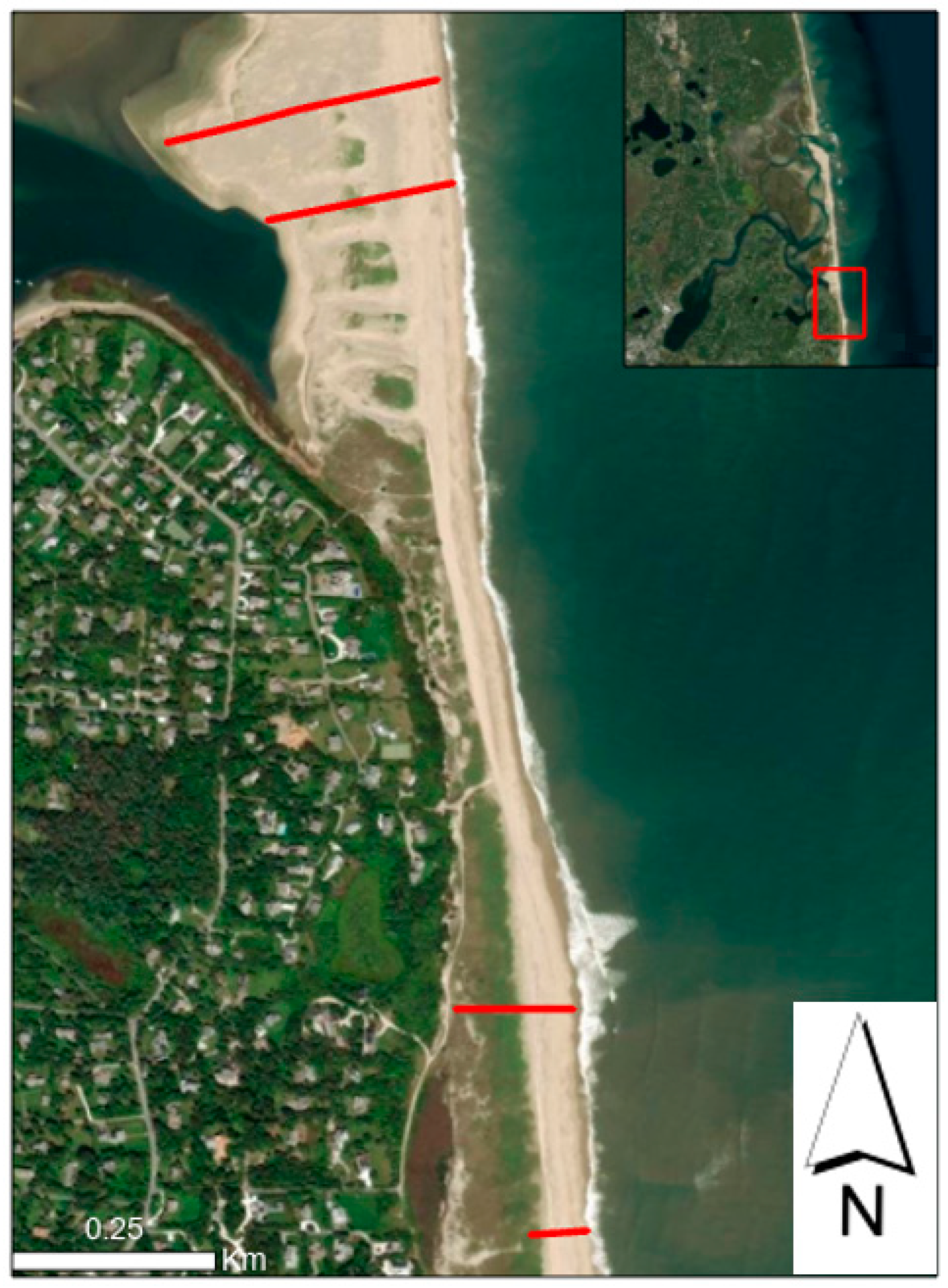
Barrier systems are vulnerable to overwash and breaching during storms [22,23,24]. While these processes are drivers of natural landward beach migration that contribute to the sustained survival of the system [20], they can also cause damages or impacts to local communities, resources, and ecosystems in the form of flooding, destruction of property, and loss of habitat. The likelihood of these processes occurring at a particular location is primarily controlled by the width, elevation, and sediment characteristics of the barrier as well as the incident wave characteristics (height, period), and elevation and duration of surge during the storm event [17,18,24,25]. Understanding and predicting beach erosion, overwash, and breaching is important for developing coastal protection and response strategies, and numerous numerical and conceptual models have been developed and applied for this purpose [18,26,27,28,29,30,31,32,33].
Geomorphic changes to sandy beach and dune systems exhibit substantial alongshore variability. Areas that display particularly severe erosion relative to adjacent areas, termed erosional hotspots, are of particular interest within the context of coastal management, and can be the result of oceanographic, geologic or anthropogenic factors [34]. More specifically, areas of high erosion may be related to offshore or onshore geology [35], wave focusing influenced by nearshore or inner shelf bathymetry [36], and the evolution and migration of the configuration of the beach and nearshore features [37], while anthropogenic causes of erosional hotspots include engineered inlet channels, beach nourishment, and nearshore pit dredging [34,38]. Identifying the primary drivers of enhanced erosion in a particular location can help predict vulnerabilities and inform resilience strategies.
The use of remote-sensing data, including aerial imagery or LiDAR acquired by aircraft or satellite, is commonplace for examining coastal change [39,40]. The use of unmanned aerial systems (UAS) for this purpose has also become widespread due to their versatility and relatively low operating costs [41]. The generation of elevation surfaces from UAS imagery using a technique called structure from motion (SfM) has become a popular alternative to LiDAR (e.g., [42]). The method for creating a 3D surface using SfM relies on identifying overlapping stationary features in multiple images, then triangulating their locations in 3D space based on camera position and the size and location of the overlapping features within the imagery [43]. This technique has been shown to be capable of generating elevation surfaces with vertical accuracies equivalent to LiDAR surveys [44], and because only a single sensor is required to capture both imagery and elevation, it is generally cheaper and more time efficient than using LiDAR. Due to the advantages discussed above, UAS-derived imagery and SfM were employed in this study to observe and quantify coastal change.
Hydro-morphodynamic modeling provides valuable insights into coastal hydrodynamics and sediment transport processes occurring along the coastline. XBeach is a state-of the-art model particularly suited to simulate the relevant processes occurring along sandy coastlines [28], including dune erosion, overwash and sediment transport [21,25,45]. XBeach model inputs include a pre-storm digital elevation model, a spatially varying friction grid, a grid indicating non-erodible features within the modeling domain, time-varying wave and tide boundary conditions, and summary bed composition properties (D50 and D90 grain-sizes) of the beach. Beyond the influence of these data inputs, performance of the model is affected by the model’s wave asymmetry parameter (referred to as facua or γua) and breaking intensity parameter beta (β) [28,30,31]. Facua controls the onshore–offshore wave-induced transport through the asymmetry of the bottom particle velocity (ua) between wave crest and wave trough, where a higher value increases the asymmetric onshore sediment transport, resulting in lower erosion rates [46]. The beta parameter controls wave dissipation through breaking in the model, where higher β values cause increased energy dissipation and, as a result, lower undertow velocity, and thereby less simulated erosion [28]. The optimal values of these parameters differ between study areas, and sub-optimal values can result in inaccurate estimates of shoreline change. Once calibrated using site-specific data, XBeach has proven to be an effective tool to predict beach barrier systems changes during storms [28,42,43,44].

1.2. Study Area

Outer Cape Cod (OCC) is an approximately 40-mile-long sandy peninsula on the eastern coast of Massachusetts (Figure 1) that is mainly comprised of sediment deposited during the melting of the Laurentide ice sheet between 20,000 to 18,000 years BP and has since been reworked to its modern morphology [47]. Many of the modern characteristics of the Cape developed within the last 6000 years, including the formation of barrier spits and embayments between 6000 and 4000 years BP [47,48] followed by the appearance of salt marshes in many areas throughout coastal New England roughly 4000 years BP [49,50], which have remained important, highly dynamic, features along of the coastline. Currently, Cape Cod is home to a year-round population of nearly 230,000 people [51] and is a popular summer tourist destination, with the Cape Cod National Seashore (CCNS) hosting approximately four million visitors per year [52]. The particular focus of this study was on the eastern ocean edge of the towns of Eastham and Orleans in OCC, consisting of portions of Nauset Beach and Nauset Bay (Figure 1).
Nauset Beach is part of the OCC littoral cell, which extends from Provincetown to Monomoy [53]. Over recent decades, this region has displayed net erosion and shoreline retreat [54], with much of the beach displaying average recession rates of more than 2 m/y over the last three decades [55]. High-energy storm events are the primary periods of barrier sediment dynamics [19]; however, sediment movement does not always yield net erosion. Average annual shoreline change rates are commonly reported for coasts over time, but these do not often capture event or seasonal dynamics and drivers. The morphology of Nauset Beach, and OCC in general, is very dynamic, and measurements have revealed “reversing storm hotspots” (RHS) along beaches between Eastham and Provincetown [38]. These RSH show severe erosion during storms and rapid accretion following the events and occur at spots adjacent to similar areas which However, show little geomorphic change during the same events. The study area also contains a migrating inlet that, since the 1950s, has undergone several cycles of northward migration; each commenced by storm-induced breaching near the pre-1950 location [56,57]. The last breach of this kind occurred in 1990, and since 1996, the inlet has migrated >1.6 km (1 mile) to the north [57]. Concern has been raised about the potential of a recurrence of breaching and the effects this might have on local erosion, shoaling and hydrodynamics.

2. Materials and Methods

This project employed a combination of historical data analysis, field observations, and modeling to evaluate morphological dynamics, including short-term responses to recent storm events and potential impacts of future storms with SLR. The hydro-morphodynamic modeling domain covers the entire area shown in Figure 1, expanding over 10 km of shoreline; the survey area, where field observations were collected by aerial imagery or surveys expands on the section circled in red, south of the inlet in Figure 1.

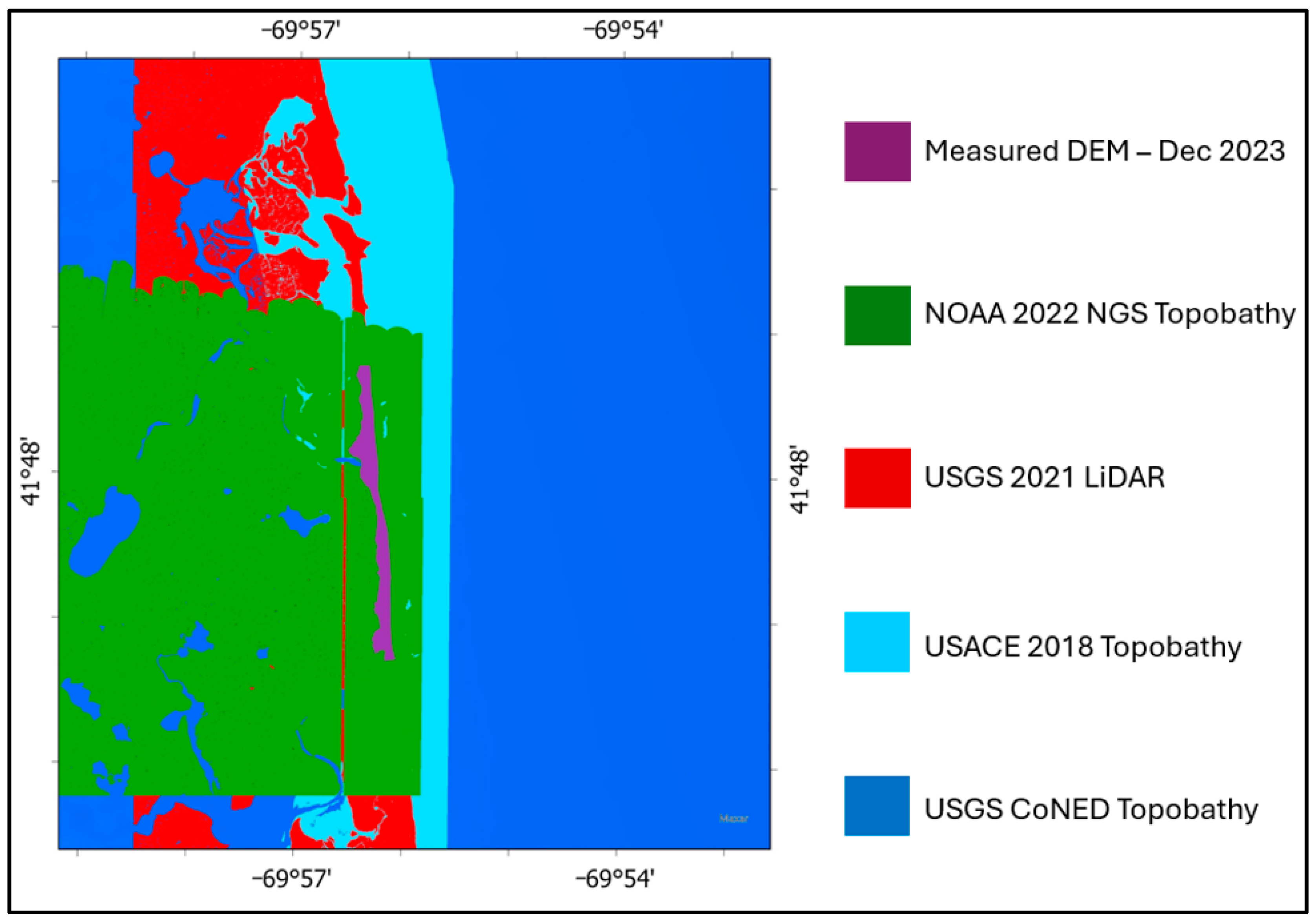
2.1. Historical Data

Publicly available historical imagery and Digital Elevation Model (DEM) datasets were analyzed to identify changes in the study area since 2011. Aerial imagery datasets from 2023, 2021, 2019, 2013/2014, and 2011 were acquired from MassGIS and Digital Globe and visualized in ArcGIS Pro V3.1. Imagery was used to qualitatively identify physical changes (i.e., overwash, inlet migration, vegetation changes) in the study area. DEM datasets from several sources were accessed through the NOAA data access viewer [58] to assess annual to decadal topographic changes between 2011 and 2021. Four LiDAR-derived DEMs or topo-bathymetric datasets of the study area were acquired from 2011, 2013/2014, 2018, and 2021, respectively. These datasets were originally collected by either USGS (2011, 2013/2014, and 2021) or USACE (2018) and all have a reported horizontal accuracy of 1 m or less and subaerial vertical accuracy of 10 cm or less. Raster datasets of elevation change between each consecutive timestep, as well as between 2011 and 2021, were created by subtracting the elevation values of the older dataset from the younger dataset on a cell-by-cell basis using the Minus tool in ArcGIS Pro. The elevation change datasets were visualized to evaluate geomorphic evolution.

2.2. Data Collection and Processing

2.2.1. Mapping

Drone-based aerial surveys of the study area were conducted on 6 September 2023, 15 December 2023, 23 January 2024, and 14 March 2024. These surveys were conducted to monitor event-driven and seasonal changes to the system, as well as capture short-term storm-induced changes to the beach. The surveys were conducted using a DJI Matrice 300 RTK quadcopter equipped with a Zenmuse P1 RGB camera (DJI, Shenzhen, China) with a full-frame 45-megapixel sensor and global shutter. The camera used a 35 mm lens with an F2.8 aperture and a 63.5° field of view. The camera was connected to an integrated 3-axis gimbal and was affixed to the drone using the DJI SKYPORT Mount (DJI, Shenzhen, China).
Mission planning, flight control, and image triggering for the aerial surveys were all conducted using the DJI Pilot 2 App. The ~1.2 km2 area of interest was covered over 4–5 flights during each survey day depending on ambient temperature and wind conditions. The drone was flown at an altitude of 120 m (400 ft) and captured images with an 80% frontal overlap and 70% side overlap. Roughly 2100 images were collected per site visit with each image capturing 120 m × 80 m of the ground surface. All flights were conducted in accordance with U.S. FAA Part 107 regulations and with permission from the Town of Orleans, MA. A minimum of six black-and-white-checkered ground control targets, which are easily identifiable in the imagery, were placed throughout the study area before each flight, and their locations were recorded using either a Bad Elf Flex Extreme (Bad Elf LLC, West Hartford, AZ, USA) or Trimble R12 GNSS system (Trimble, Westminster, CO, USA) used as a Real-Time Kinematic (RTK) GPS which received real-time corrections via Massachusetts Continuously Operating Reference Station Network (MaCORS). The ground-control-point coordinates were used to georeference the imagery mosaics and DEMs produced from the collected imagery.

2.2.2. Producing DEMs from Drone Imagery

Following each round of data collection, an orthomosaic and high-resolution (1.5 cm per pixel) DEM was generated from the acquired imagery using Pix4D Mapper v4.8.4. First using Pix4D, the imagery was mosaicked and georeferenced using the ground-control points. SfM analysis was performed to produce a DEM of the survey area which was then transferred into ArcGIS Pro as a raster dataset. Because SfM-constructed DEMs rely on overlapping stationary features in multiple images, areas over water and along the edges of the mapped area (where imagery was sparse) are prone to inaccuracies [59]. These were removed using the mask by extent tool in ArcGIS Pro. Additionally, SfM-produced DEMs have potential elevation errors due to vegetation, and as a result, the change analysis presented in this paper is focused on areas with little to no vegetation.

2.2.3. Ground Surveys

On each survey date, four cross-shore elevation transects were taken using a Trimble R12 RTK at select locations along the study area (Figure 2). The transects were compared over time to assess beach evolution at the selected locations throughout the study period. Additionally, they provided additional confirmation of the SfM-created DEMs. Transects were also compared to historical LiDAR using the Extract Surface Information tool in ArcGIS Pro to examine long-term beach evolution at those same locations.
To assess the spatial and temporal variability of the sediment texture of the study area, surface sediment samples were collected along each of the transects during each site visit, and locations were recorded using a Trimble R12 RTK GPS. A minimum of four samples were collected per transect during each visit, with 81 samples being collected in total. In the lab, all samples were homogenized by hand in their sample bags, dried overnight in a drying oven at 60 °C to remove moisture content, weighed, sieved at 2 mm, and weighed again to determine the sand and gravel percentage by mass of each sample. Grain-size distribution of the sand portion (<2 mm) in each sample were determined using a Malvern Panalytical Mastersizer 3000 (Malvern Instruments Ltd., Malvern, UK).

2.3. XBeach Modeling

2.3.1. Model Setup and Calibration

The topobathymetric data used for the XBeach simulations were based on a combination of topographic and bathymetric data: the constructed 15 December 2024 DEM was combined with topobathymetric data from 2022 (NOAA NGS Topobathy LiDAR [60]), 2021 (USGS LiDAR [61]), 2018 (USACE NCMP topobathy LiDAR [62], and the USGS CoNED Topobathy DEM [63]). These datasets were combined using the Mosaic to New Raster tool in ArcGIS Pro with the most recent data being used in any areas of overlap (Figure 3). The newly created raster was generated with a 5 m resolution.
The non-erodible and friction data used in the model setup were derived from the 2021 NOAA C-Cap Version 2 Impervious Cover [64] and 2016 NOAA High Resolution Land-Cover datasets [65], respectively. Land cover classifications were converted into Manning coefficient values using the standard conversion land cover classification-Manning values [66] to create a spatially varying friction layer.
The XBeach coastal computational grid was designed with a variable resolution between 20 m to 5 m, with the lower resolution offshore and the higher resolution onshore. The topo-bathymetry, the friction and the non-erodible layers were both interpolated on the computational grid to be used in XBeach simulations.
The storm events were first simulated with the mean circulation model ADCIRC fully coupled with the wave model SWAN, which used data from the European Centre for Medium Range Weather Forecasts (ECMWF) reanalysis product ERA5 [67] for its meteorological forcing. Predicted waves, tide, and storm surge values with this model were extracted at the offshore boundary of the coastal grid to be used as offshore boundary condition for XBeach. The local grain size characteristics were based on samples collected on 15 December 2023 at the site.
The model was calibrated based on morphological changes observed between the drone-derived DEMs collected on 15 December 2023, and 23 January 2024. During this period, two significant storm events impacted the study area: a winter storm that occurred on 18 December 2023, and a cluster of consecutive storms that struck Cape Cod between 7 January and 14 January 2024. Since both events had a significant impact on the morphology of the study area, they were simulated consecutively to calibrate the model based on the observations. The calibration involved optimizing the two XBeach parameters, the factor of wave asymmetry (facua [γua]) and the rate of wave energy dissipation at breaking (beta [β]) to minimize the errors between observed and simulated subaerial erosion.
The numerical simulation of the 18 December 2023 winter storm modeled the storm during 48 h, from 12:00 AM December 17 to 12:00 AM 19 December 2023. Time series of significant wave height and mean water level (MWL) computed for this storm (using ADCIRC-SWAN) along the offshore boundary of the XBeach domain are shown in Figure 4 The predicted morphology after this initial storm was used as the initial condition for the simulation of the next storm events that occurred in January 2024. This was a cluster of storms that lasted from 8:00 AM 7 January to 12:00 AM 14 January 2024 (see Figure 4 for wave height and MWL time series for these storms). The final simulated morphology was compared to the morphology observed on 23 January 2024.
To calibrate the model, this sequence of storms was run with several different combinations of the two parameters, γua and β parameters, with γua values ranging from 0.2–0.28 and β values ranging from 0.05–0.1. The performance of the model was evaluated based on the comparison between simulations and observation of (1) the subaerial sand volume change (m3/m), (2) skill of the modeled distribution of erosion, which was defined by the spatial accuracy of the predicted occurrence of erosion compared to the observational data (see Appendix A) and (3) visual comparison of elevation-change patterns compared to observations. The γua and β values of the calibration simulation with the best overall performance were deemed to be γua = 0.24 and β = 0.07 and were used in all subsequent simulations (see Appendix A). When evaluating model performance, only data located within the mutual extent of the measured 18 December and 23 January DEMs was considered (purple area in Figure 3).

2.3.2. Modeling the Influence of Wave Direction and Bathymetry on Subaerial Erosion

To assess the sensitivity of the morphological response to the wave direction, additional simulations of the cluster storm (18 December 2023 to 14 January 2024) were performed, varying the wave direction to 230°, 270° (shore normal/default), 310° and time-varying wave directions as provided by the ADCIRC-SWAN simulations.
Furthermore, observations in Google Earth and other aerial imagery revealed that the nearshore sand bars in the study area appeared to have shifted southward since 2022 (i.e., the year of the most recent topobathymetric data used for the model grid). To test the influence of the bar movement on erosion patterns, the subaqueous portion of the model elevation grid was uniformly shifted 300 m southward, and simulations were rerun using the same storm data and boundary conditions.

2.3.3. Modeling the Effects of Sea-Level Rise on Storm Impacts

XBeach was also used to simulate the potential impact of such a cluster storm under higher sea level conditions. To this effect, the storm was simulated with 0.30 m (1 ft) of increased sea level, a forecasted average magnitude of SLR in the study area by 2050 [5]. In this scenario, the model similarly used the optimized γua and β parameters and same data sources and model setup as described. No attempt was made to account for potential morphological changes the area might undergo by 2050 or any management actions (e.g., dune plantings).

2.3.4. Model Limitations

Like every model, XBeach is subject to limitations. First of all, XBeach’s physics is simplified [28], with its wave model being phase-averaged and neglecting reflection and diffraction among others. Earlier work in comparison to models with extended physics, however, have shown that XBeach performs adequately for highly dissipative sandy beach barrier systems [32]. In applying the model, perhaps most notably, XBeach requires accurate observations of the current geometry of the system, therefore out-of-date or poor quality topographic and bathymetric inputs, which do not represent the current state of the system, will lead to inaccuracies in predicted storm responses. Also, while the model does incorporate landcover type and sediment composition, it assumes uniform sediment composition, and a landcover classification may not accurately reflect the type/magnitude of vegetation present; therefore, the model cannot fully capture the complex influences of variable sediment composition vegetation during storm events. As performed in this study, XBeach must be calibrated using site-specific response to actual storm events, hence, the calibration is only valid for similar events; and XBeach relies on hydrodynamic inputs that were derived from another model (ADCIRC-SWAN), which is subject to its own limitations and uncertainties in its own input data (i.e., here the synoptic storm parameters). Finally, due to the complexity of the model, running XBeach with fine spatial resolution or on large areas is extremely computationally expensive. Therefore, the resolution of the XBeach grid used in this project is quite coarse (5 m cells) compared to other geospatial datasets used in this project. Despite these and other limitations, XBeach is a well-established tool capable of predicting general barrier systems changes during storms [32].

3. Results

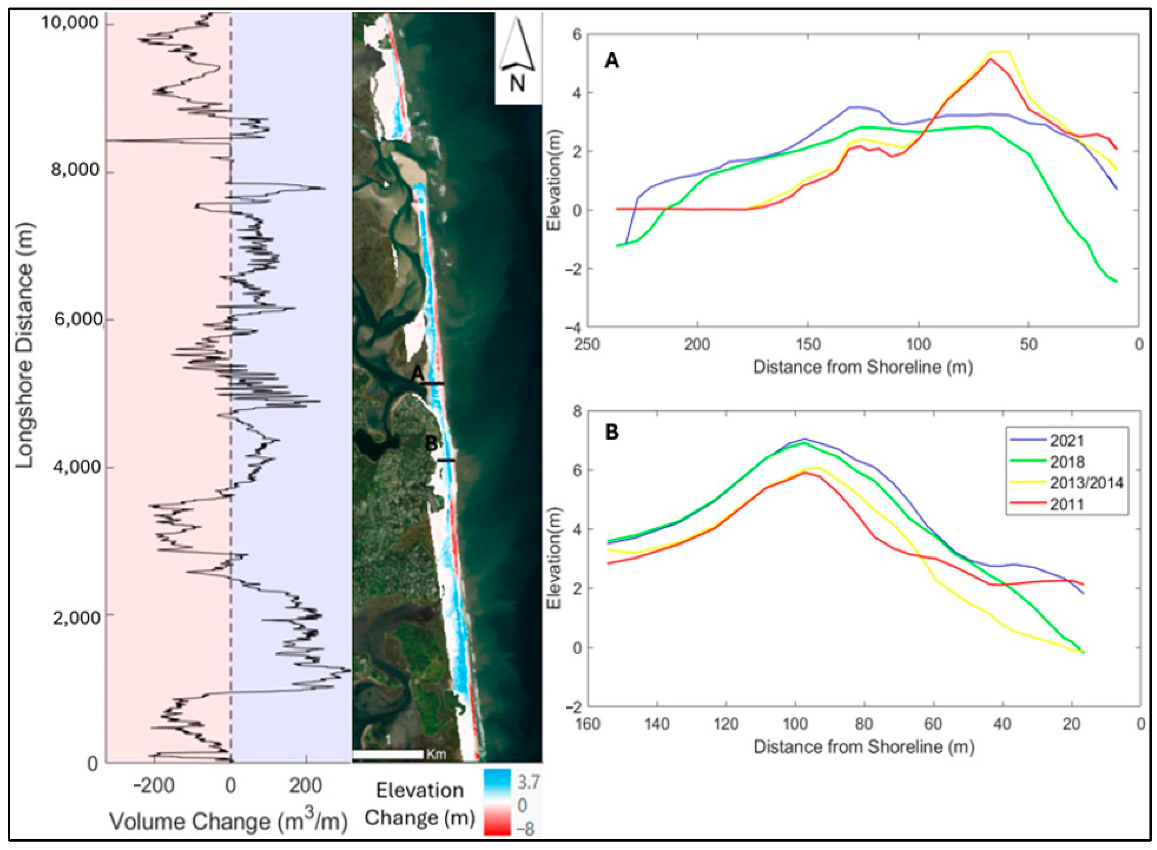
3.1. Long-Term Morphological Changes

Analysis of historical LiDAR and aerial imagery since 1996 illustrated clearly how the morphology of the study area has significantly changed over recent decades. Physical changes to the beach dune system can be identified in historical imagery in the form of overwash fans, dune loss and recovery, and the migration of nearshore bar features (Figure 5). Given the dynamics visible in the system, the net difference in the total volume of the subaerial portion of the study area between 2011 and 2021 was surprisingly small, with a slight increase in the average volume (11 m3/m) (Table 1). However, during this interval the three-dimensional shape of the beach was significantly altered (Figure 5), with eroded areas experiencing a total of 86.6 m3/m of volume loss and accreted areas totaling 97.7 m3/m of volume gain. The area also displayed significant temporal variability in beach volume, losing 53.5 m3/m of beach volume between 2011 and 2014, and then subsequently accreting a similar volume (49.4 m3/m) from 2014 to 2018.
While total beach volume displayed spatial and temporal change in accretion and erosion, dune volume (classified here as areas of the beach > 3 m in elevation) showed consistent volume loss since 2011 especially along the spit (e.g., Figure 6, Transect A), and this is visible in the aerial imagery as a decrease in the vegetation extent since 2013 (Figure 5). In fact, the total dune volume decreased between every measured timestep, with a net change in dune volume of −31.8 m3/m (Table 1). The map of elevation changes between 2011 and 2021 displayed a general pattern of foreshore and dune erosion and accretion of the backshore and, in some areas, landward (Figure 6). But there was significant alongshore variability that tracks similarly to alongshore volume changes (Figure 5 left side). Both dune and beach erosion were highly spatially variable. The southern portion of the spit, for example, experienced overwash, which flattened the dune and deposited a thick (~1.5 m) layer of sediment backshore (Figure 5 in 2019; Figure 6, Transect A), followed by gradual landward recovery of dunes (Figure 5 in 2021–2023; Figure 6, Transect A). During the same time interval, the dunes on Transect B, about 1 km to the south of Transect A, experienced consistent accretion and progradation (Figure 6, Transect B).

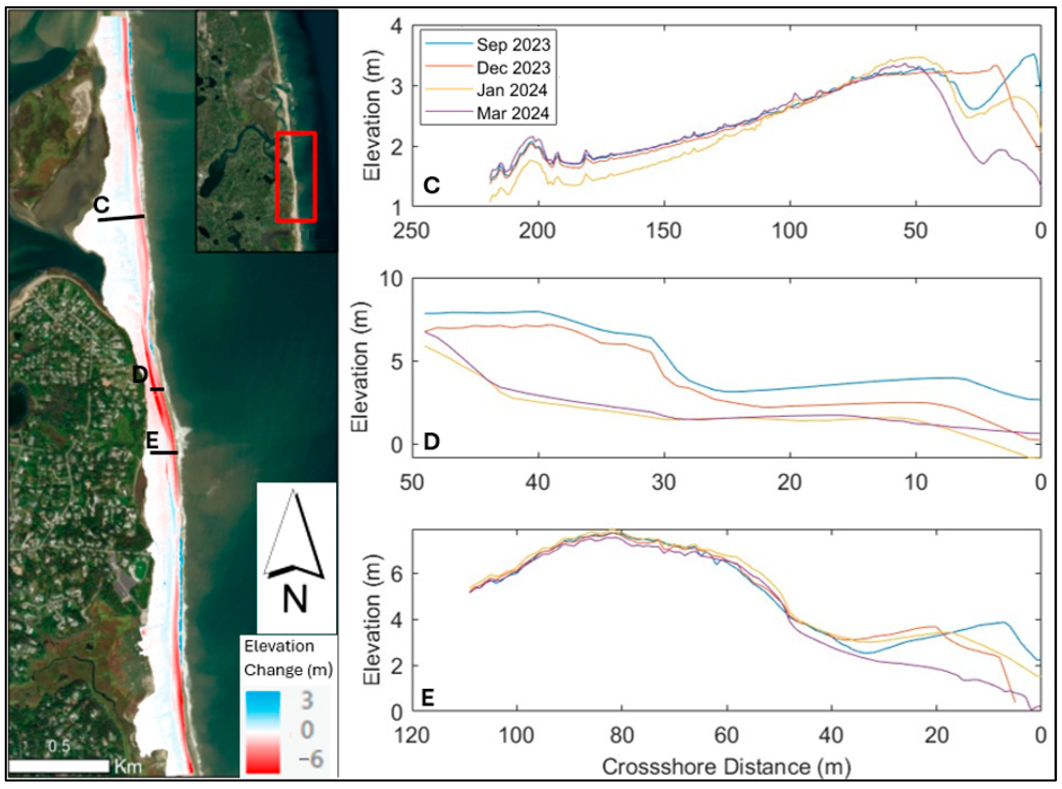
3.2. Winter 2023/24 Beach Evolution

The drone-surveyed portion of Nauset Beach (see Figure 3) experienced net erosion between every survey conducted during the study period. Over the 2023–2024 winter (6 September 2023, to 14 March 2024), the subaerial volume of this area decreased by 44.9 m3/m. The greatest and most rapid volume loss occurred during the interval from 15 December–23 January, during which time the survey area lost 22.3 m3/m of sediment (Table 2). This interval corresponded to the stormiest portion of the winter in the region, with four significant storms impacting the study area during that time (Figure 4). The first event during this window was a large nor’easter, which traveled up the east coast on 17–18 December, resulting in heavy rain and winds and causing widespread flooding, power outages, and property damage throughout coastal New England [68]. In Cape Cod, a NOAA wave buoy located north of Provincetown recorded sustained wind speeds greater than 20 m/s (39 knots) with over 27 m/s gusts (52.5 knots), and significant wave heights exceeding 4 m on 18 December [69]. The study area then experienced a series of three additional strong storms on 7, 10, and 13 January. These storms also caused heavy rain, snow, and wind throughout New England as well as significant flooding and structural damage [70]. At the Provincetown wave buoy, peak sustained wind speeds reached 19 m/s (37 knots) with gusts greater than 26 m/s (50.5 knots) during the 10 and 13 January storms, while the January 7 storm had sustained wind speeds up to nearly 16 m/s (31 knots) and gusts of 20 m/s (39 knots) [69]. During all three of these events, offshore significant wave heights exceeded 4.8 m at the Provincetown wave buoy, with the highest waves (exceeding 5.3 m) occurring during the 7 January event [69].
Significant spatial variability of morphological change was observed over the full study period. Most of the erosion appeared to be along the foreshore while the dunes were less impacted (Figure 7). Transect C in Figure 7, for example, shows significant erosion of the beach face but with slight accretion of the dune. However, considerable dune erosion is evident at other locations along the coastline. The area immediately south of the spit (Figure 7, Transect D) stood out as an area of particularly severe erosion, losing 144.5 m3/m of sediment at Transect D over the study period. Much of this erosion likely occurred during the storms between 15 December and 23 January; as substantial change (−103.8 m3/m) was measured over that period. From January to March, the erosional hotspot exhibited a small net recovery of the lost volume (e.g., 16.3 m3/m at Transect B). Some accretion was observed in the area immediately south of the erosional hotspot (i.e., in the vicinity of Transect E, Figure 7) from September to January, but this location eroded significantly between January and March.

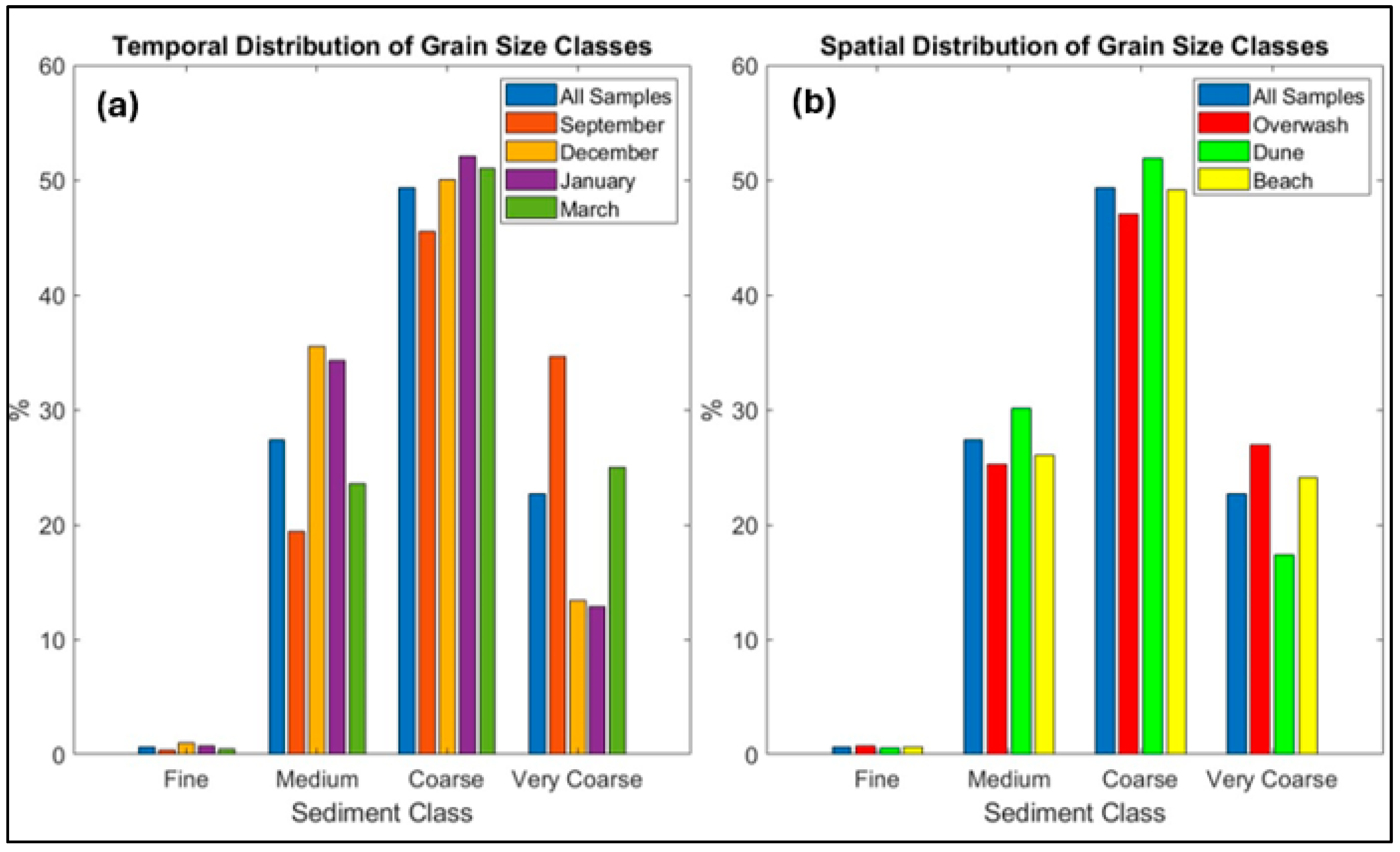
3.3. Sediment Composition

The surface sediment composition of Nauset Beach was primarily coarse to very coarse sand with a small proportion (~2% by mass) of gravel-sized particles. The study area was dominated by coarse sand with >20% of medium and very coarse sediment overall (Figure 8); however, some spatial and temporal differences in the grain- size distributions were observed. The average median grain size (D50) of all the collected samples was 816 µm. Sediments collected from overwash fan areas had higher median grain sizes (mean D50 of 847 µm), likely due to higher percentages of very coarse and gravel sediment. Samples collected on dunes (>3 m elevation), on the other hand, had finer grain sizes than beach and overwash areas (a mean D50 of 756 µm was observed for dune sediments) and contained virtually no gravel-sized particles.
Sediment sizes in the survey area also displayed temporal variability (Figure 8). Average median grain size was highest in September, with samples collected in September having an average D50 of 955 µm. The largest change in measured grain sizes occurred between September and December, when the average median grain size reduced to ~700 µm, the period of finest measured sediment (Table 3). From December to January, the distribution of sand-sized sediment was relatively unchanged. Then, between January and March, the average D50 increased, but the median grain size in March was still ~100 µm smaller than in September. In Table 3, overwash samples include all samples collected along overwash fan transects, dune samples include all samples collected at elevations > 3 m, and beach samples include all samples collected seaward of the dune toe.

3.4. Modeling Results

XBeach simulations of the storms that occurred on 18 December and 7–14 January (see Figure 4 for offshore forcing) predicted a cumulative subaerial volume loss in the survey area of 24.1 m3/m. This prediction agreed well with the 22.28 m3/m of net sediment loss observed between 15 December and 23 January for the same area from the drone DEM data (Table 4). The model also predicted reasonably well the spatial distribution of erosion (see Appendix A). However, while total volume change was similar to the observations, the simulations underestimated both erosion and accretion by a similar amount (Table 4) and predicted a small overwash event that did not occur (Figure 9). Additionally, the simulations failed to predict the location of the pronounced erosional hotspot observed immediately south of the spit near Nauset heights (Figure 10, Transect B). The model did, however, simulate an area of high erosion a few hundred meters north of where the erosional hotspot was observed, but this simulated hotspot predicted less erosion than was observed at the mapped hotspot (Figure 10, Transect F).

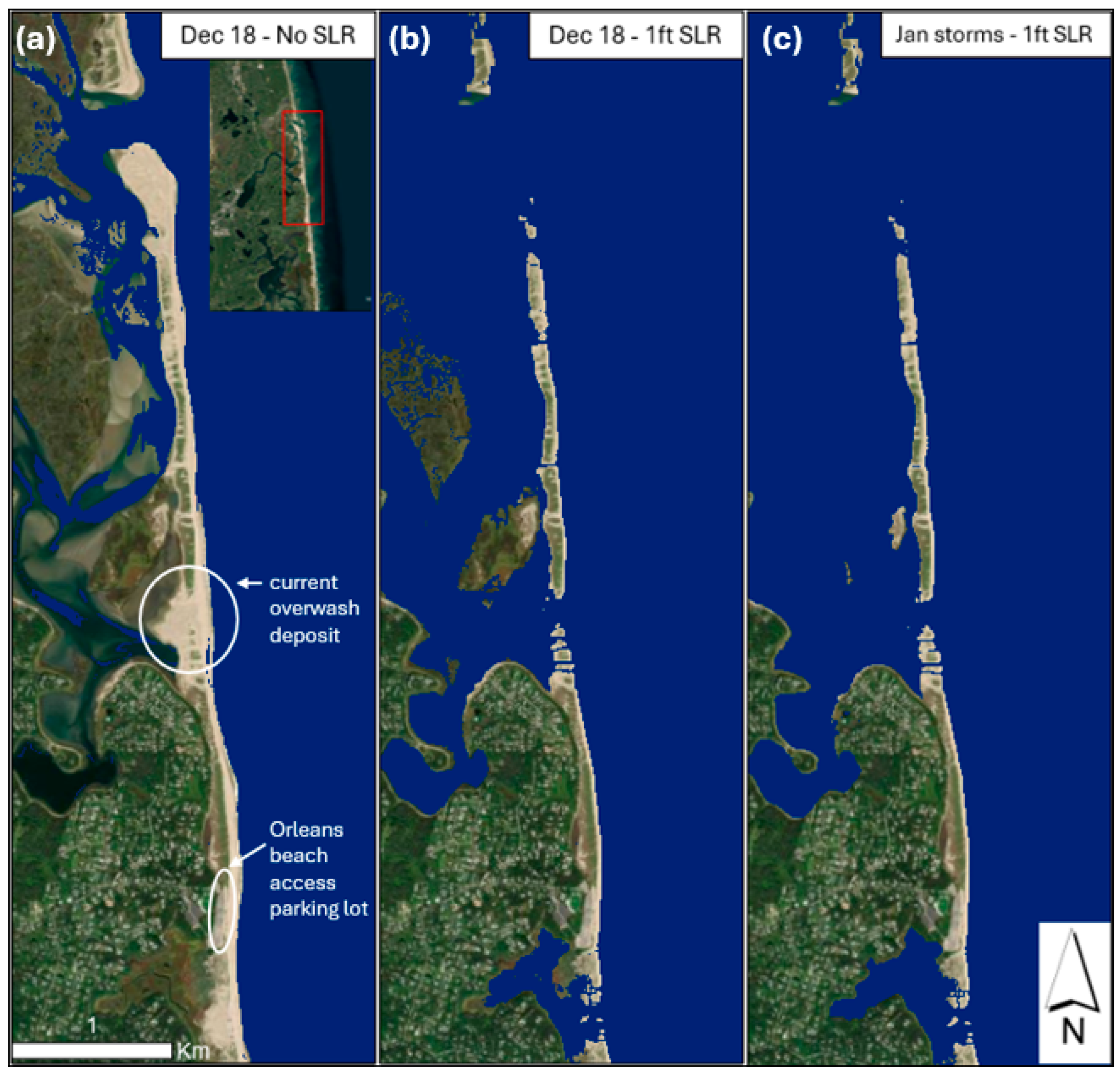
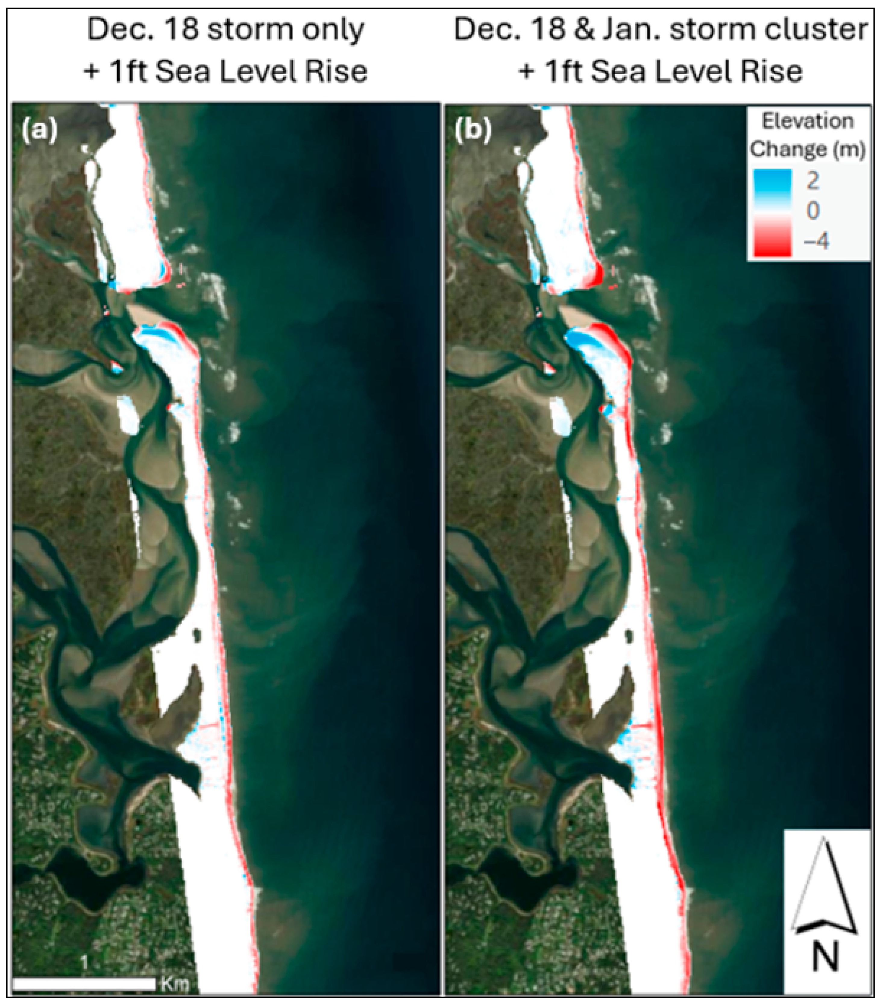
Sea-Level Rise Simulations

The XBeach simulation of the December 18 winter storm under 0.30 m (1 ft) of SLR predicted a significantly greater inundation of the study area (Figure 11). While patterns of erosion similar to the simulations of modern conditions were predicted (Figure 12), larger sediment movement and subaerial volume loss were observed; with the added sea level, 16.1 m3/m of net subaerial sediment loss was predicted during the 18 December event.
Maximum water levels overtopped the barrier in several locations along the spit, resulting in dune breaches (Figure 11) and overwash deposition landward of those locations (Figure 12). As in previous simulations, the model predicted heightened erosion and overwash where the current overwash fan is located, on the southern portion of the spit (Figure 12). It also forecasted erosion and widening of the Nauset Bay inlet.
In the simulation of the January storm cluster with SLR, inundation pathways mirrored those of the December simulation (Figure 11), causing the expansion and deepening of dune breaches that formed during the December 18 simulation. This occurred most notably at the location of the existing overwash fan (Figure 12), although overwash was also indicated near the inlet and south of the Town of Orleans beach access parking lot (indicated in Figure 11). The primary dune breach located on the southern end of the spit, which was initiated during the December storm, was eroded to elevations of less than 1 m (above the simulated MWL). So, while the model did not predict a complete breach during these events, enough elevation was removed to connect Nauset Bay and the ocean during typical high tides at this location under the simulated sea level conditions. Overall, the consecutive simulations predicted a total of 33.3 m3/m of subaerial sediment loss in the survey area, about 50% more than the net volume lost observed in the drone DEMs between 15 December and 23 January.

4. Discussion

4.1. Storm-Driven Beach System Evolution

The role of storms as primary drivers of morphological changes to barrier systems and other beaches is well established [17,19]. Hurricanes and winter storms (e.g., nor’easters) are the primary erosion threats to New England, with various types of extratropical coastal storms being common along the U.S. East Coast [71]. The fundamental influence of storms on shoreline morphology was evident in both the historical data from 2011–2023 and in the observations of seasonal volume changes of the study area during the winter of 2023–2024. Morphological data revealed the constantly evolving nature of the study area, with the most significant changes associated with recent and past large storm events.

4.1.1. Historical Storm Impacts (2011–2021)

Since 2011 and prior to 2023, the study area has been affected by several major storms, most notably Hurricane Sandy in 2012 October [72], a nor’easter in January of 2015 [73], and two large nor’easters in January and March of 2018 [74]. Sandy caused significant erosion near the Town of Orleans beach parking lot and along the southern end of the Nauset Bay spit. USGS research indicated extensive collision (following classification of Sallenger, 2000 [18]) and some overwash and inundation along OCC and around New England [75]. Overwash was also significant during the 2018 nor’easters, which caused widespread flooding along with home and infrastructure damage. In total, the 2018 storms are estimated to have caused 31 deaths and more than 3.3 billion dollars in economic loss in the U.S. [75,76]. Additionally, a large geomorphic impact was experienced on the barrier-portion of the study area. Coastal changes in the study area from the 2018 storms were in the form of dune erosion and overwash fan deposition which are evident in the historical imagery (Figure 5). In subsequent years, both imagery and LiDAR data indicated gradual dune and vegetation recovery landward of the pre-storm dune locations (Figure 4 and Figure 5). Interestingly, historical LiDAR data taken after the 2018 storms revealed a net gain in sediment volume in the study area compared to the 2013/2014 dataset (Table 1). Resilient coastlines have been observed to gain volume despite heavy storm activity [77]. However, because this area has not historically displayed net accretion during stormy conditions, and a net loss of dune volume was observed during this interval (−6.6 m3/m, Table 1), it is possible that the measured net volume gain across the system from 2014–2018 represents seasonal beach accretion.
Dune erosion of barrier beaches generally occurs during storms when wave runup exceeds the dune toe elevation [18,78], and research has shown that eroded dunes do not recover quickly, as aeolian accretion is normally slow [79,80]. In this study, net dune erosion was observed between every timestep of the historical LiDAR data examined. The DEM data suggests that while the study area appears to have roughly maintained its total sediment volume, the dunes are losing elevation. Dune recovery is generally controlled by several factors including sediment supply, vegetation regrowth, pre-storm dune geometry, nearshore features, and storm frequency/magnitude [80]. While all these factors may have some impact on longshore differences in dune recovery, the net loss of dune volume over the 10-year study period suggests that the dunes lack sufficient time to recover under the recent storm magnitude and frequency. Historical data also reveal long-term trends of net landward sediment transport within the study area. The foreshore and dunes generally lost volume between 2011 and 2021, while the backshore gained volume (Figure 6). This combination of change is symptomatic of barrier rollover, associated with landward migration [17,20]. Unimpeded landward migration might allow for the persistence of the barrier with SLR, but throughout the OCC and along barrier systems globally, a consistently landward migrating beach will eventually encroach upon recreational and residential assets, and ultimately affect future storm-driven flooding and infrastructure damages.

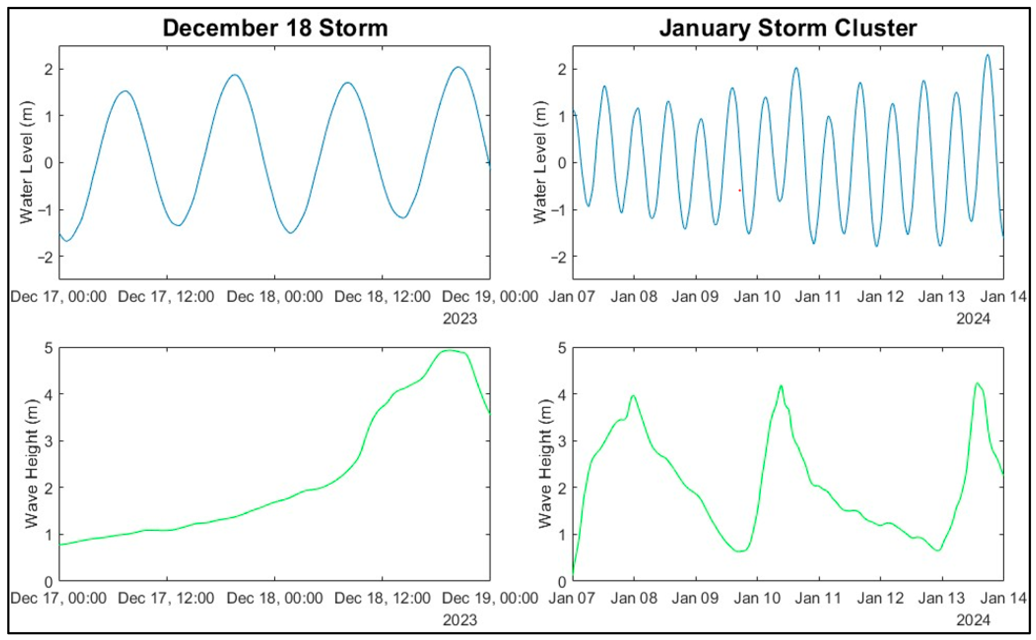
4.1.2. Impacts of Successive Winter Storms

Stormy periods when successive storms affect coastal areas are often discussed as problematic to communities, but limited research has quantified their effects. Observations (and modeling, discussed below) of the study area throughout the 2023–2024 winter highlight the erosive nature of the storms during the higher energy winter months as well as severe changes during short-term events. Between September 2023 and March 2024, southern New England including OCC experienced multiple storms including Hurricane Lee in mid-September, a nor’easter on 18 December 2023, and a series of three winter storms on 7, 10, and 13 January 2024. During this time the survey area eroded on average more than 40 m3/m of its subaerial volume (Table 2). While the net change was consistent with the seasonal trend of increased erosion during the winter (typically balanced by with recovery during the summer) in New England Beaches [81], much of the observed erosion was highly focused, causing pronounced areas of major dune erosion that are unlikely to recover in subsequent years, if ever.
The December storm, the December and January storms had the greatest impact on the study area during the observation period. These storms resulted in flooding, power outages, structural damage, and coastal erosion throughout Cape Cod [82,83]. The major storms all occurred between the 15 December and 23 January field surveys over which the subaerial system eroded >20 m3/m of sediment, and the average rate of erosion was more than double the rate over the entire survey period (Table 2). The most striking geomorphic impact of these storms was an area of focused erosion highlighted in Figure 13, where portions of the dune receded roughly 20 m, removing up to 5 m of elevation. This feature eroded on the order of five times more than the average for the survey area during that period. Areas of concentrated storm-induced erosion (i.e., “hotspots”) have been observed around the world [34,35,79,84,85] including along OCC between Eastham and Provincetown between 1998 and 2002 [38]. However, monitoring by [38] showed the OCC eroded regions rapidly recovered within weeks to months following the storms. In this study, only minor recovery of the December to January hotspot erosion was observed in following months. The tendency of a coastline to experience significant dune loss or severe, localized, erosion during storms has significant implications for potential hazards and effects of future storms. For example, dune loss or localized beach erosion (i.e., a hotspot) occurring near a particular property or public asset could increase the risk of flooding or storm-induced damage during subsequent storms. Alternatively, focused dune erosion on a barrier spit in a hydrodynamically favorable inlet location might initiate a breach and subsequent inlet formation. These risks are compounded when considering groups of closely clustered storms like those observed in December and January. Here, the latter storms impacted areas already depleted of sediment by the December storm, that had little time to recover. Likely drivers of the erosional hotspot are discussed further in Section 4.2. Between January and March, the erosional hotspot recovered roughly 10% of the volume lost since September, while adjacent areas experienced erosion (Figure 13). Erosion between January and March was especially pronounced in the area immediately south of the erosional hotspot (e.g., 70 m3/m calculated at Transect C in Figure 7), which was largely accretive prior. This reversing response may suggest that the erosional hotspot served as a sediment source to adjacent depositional portions of the beach throughout much of the winter.
Another region of geomorphic interest is the southern portion of the spit in the vicinity of the overwash fan (highlighted in Figure 11). Breaching and inlet formation in this location have occurred in the past [56,57], and there is concern about the potential reoccurrence of inlet opening in this area which may induce erosion in back bay areas or shoaling in navigational zones, which is already an issue for the Town of Orleans [53,57]. During the observation period, erosion at this location was largely confined to the beach face, while the dune in this area accreted slightly (Figure 7). Similar re-growth of dunes and landward movement of sediment volume, as well as dune revegetation, have occurred since the 2018 overwash event and suggest the creation of some increased resistance to future inlet opening. Observations and modeling indicate storms of a similar magnitude and frequency to those observed during the 2023–2024 winter were not sufficient to yield even minimal breaching. Although breaching in this location is still certainly possible, under current conditions inlet opening would require a storm (or group of storms) of considerably higher intensity than those during the 2023–2024 winter season. Today, a new inlet may be more likely to open in a more northern portion of the spit, where the barrier is narrower [24].

4.2. Controls on the Observed Erosion

The alongshore variability of subaerial erosion and accretion can be influenced by a variety of factors including the geometry of the beach, wave focusing, and sediment transport influenced by the configuration of nearshore bathymetric features, and variable sediment composition of the beach [86,87,88]. Recent observations highlight the occurrence of significant, localized storm-driven erosion in the survey area (Figure 13). Understanding the factors driving focused volume loss can inform the decisions of resource managers regarding whether particular mitigation strategies, such as dune-grass planting or beach nourishment, are recommended, and where those strategies should be prioritized.
XBeach simulations of the 2023–2024 winter stormy period also predicted a region of enhanced erosion, but the magnitude of the erosion was underpredicted and the location was somewhat different (i.e., the measured maximum was 300 m south of where it was predicted) (Figure 9 and Figure 10). These modest but notable differences were hypothesized to be influenced by either the input wave direction and/or the nearshore bathymetry as both have been shown to influence longshore geomorphological patterns through their influence on nearshore wave energy [35,36,89]. In the calibrated model, the default wave direction was used (i.e., perpendicular to the beach), and the nearshore bathymetry was based on a combination of 2022 and 2018 topobathymetric LiDAR surveys (Figure 3) that were collected 1–5 years before the measured storm period. Therefore, to test the influence of both factors, XBeach simulations were re-run using various wave directions and bathymetry scenarios (see Section 2.3.2). The results of these simulations described below suggest that the configuration of the nearshore bathymetry had a primary control on the location and magnitude of the erosional hotspot.
XBeach output from the simulation using adjusted bathymetry showed a distinct improvement in the predicted location and magnitude of the erosional hotspot (Figure 14). The erosional hotpot appeared to be highly linked to an opening in the nearshore sandbars, causing higher and more energetic waves to impact the beach in this area (Figure A4). A similar relationship was observed by [36], who demonstrated alongshore sandbar configuration affected wave energy and shoreline variability in the Outer Banks of North Carolina. Previous research has also documented the correlation between sandbar configurations and erosional hotspots [35,85]. The model output in this study clearly indicates the strong control of the sandbar positioning on wave energy and the direction and magnitude of suspended sediment transport. Specifically, the modeled southward shift in the position of the sandbar break resulted in a corresponding southward shift in hydrodynamic forcings and the divergence of sediment transport which in turn was correlated to the location of maximum modeled erosion in both simulations (Figure 14 and Figure 15). These findings support the strong influence of nearshore bathymetry on subaerial erosion patterns and the importance of up-to-date bathymetric data inputs for the accuracy of XBeach models in regions with highly dynamic nearshore features.
The potential influence of alongshore variation in beach shape and sediment composition on the location of the erosional hotspot were also considered. The relationship between beach width and dune erosion is well established [17,19]. It is hypothesized that the extent of dune erosion at the hotspot was likely augmented by the narrow width of the foreshore in this area (Figure 7), allowing wave runup to impact the dunes. Aerial imagery shows that this area narrowed significantly since 2021 (Figure 5), and this was likely in response to the increased wave energy related to the shift in nearshore bathymetry. Therefore, the narrow beach face was likely a consequence and thus an additional indicator of the hydrodynamic changes rather than the primary cause of the erosional hotspot.
Spatial variability of sediment grain size can also influence longshore erosion and accretion patterns [86]. Areas of finer sediments tend to be more susceptible to erosion during storms [90]. However, sampling in the study area exhibited only minor alongshore variability in sediment grain-size. Additionally, some temporal variability in surface sediment grain sizes was noted, but no clear trend of change was apparent; coarse sands were observed to dominate the study area (Figure 8). While most sediment sampling was outside of the erosional hotspot (Figure 2), a few samples collected within it during the December survey had similar grain-size distributions to other samples (see Appendix B). Comparison of XBeach model runs that used default versus observed grain sizes showed that measured coarser sediments notably reduced the overall modeled sediment transport, but the patterns of change persisted [91]. Thus, the limited alongshore variability of sediments in the survey area (mean D50 for transects from the December collection were all between 600–800 µm) supports the notion that grain-size variations were not a significant control and reinforces the idea of bathymetric control on the location of the erosional hotspot.
As mentioned above, alongshore variability of geomorphic changes is the result of a complex interplay of physical, climatological, and oceanographic factors. Therefore, while the nearshore bathymetric influence on focusing wave energy appears to largely control the occurrence of the observed erosional hotspot, alongshore variability in storm-impacts within the study area as a whole will be controlled by a combination of focusing of wave energy, nearshore bathymetric features, and beach configuration as primary influences; as well as factors such as incoming wave direction, vegetation (i.e., abundance of dune-grass), and sediment composition as secondary influences.
The strong influence of nearshore bathymetry on both the modeled and observed subaerial morphological changes observed within the study area highlights the importance of access to high-quality, up-to-date, bathymetric data for coastal resilience assessments. However, mapping subaqueous surfaces using traditional vessel based acoustic echo sounding is time consuming and expensive, and is infeasible in the nearshore where shallow water levels prevent safe navigation [92]. Fortunately, various alternative methods have been developed to allow for efficient and accurate measurement of nearshore bathymetry. For example, nearshore bathymetry has been collected using sensors attached to small personal watercraft like jet skis (e.g., [93]) or autonomous vehicles (e.g., [94]). Additionally, nearshore bathymetry can be obtained using depth inversion based on wave theory using videos or images of the water surface [95]. Imagery for depth inversion has been collected using various methods including shore-based cameras (e.g., [96]), aerial surveys (e.g., [97]), and satellites (e.g., [98]). These techniques allow for relatively inexpensive and repeatable measurement of the nearshore bathymetry, which could be included in coastal resilience and modeling studies where budgeting is possible.

4.3. Storm-Impacts with Sea-Level Rise (SLR)

A foremost concern among stakeholders locally and globally is how the coastal system will respond to rising sea levels and associated storms [33]. It is well understood that increases in relative sea level will increase the frequency and duration of storm-induced flooding as well as increase the potential for storms to erode and reshape the beach system [6,7,33,99]. The OCC region is likely to experience roughly 0.30 m (1 ft) of SLR by the early 2050s (see Figure 2.3 in [5]). With a well-performing model, this study simulated the December and early January storms in XBeach with SLR. It is important to remember, however, that these models simulate the impact of storms on the system if both current bed levels and storm climatology remained the same. This is, of course, unrealistic as the geomorphology of the system is constantly changing in response to the hydrologic conditions, and coasts will adjust/reshape over time in response to SLR as highlighted by Brunn Rule modeling and other work (e.g., [33,100]). Additionally, future storms may become more intense [101,102]. Therefore, outputs from these simulations are not intended to identify specific areas of vulnerability or storm-induced morphological impacts on the coast, but rather capture general patterns and processes that the study area will experience during storms with higher sea levels.
Results from the simulation of the December storm with SLR demonstrate a likelihood for increased storm-driven erosion and overwash frequency. Unsurprisingly, higher sea levels resulted in greater subaerial erosion during the modeled storm, and substantial overwash was predicted, particularly at the location of the current overwash fan (Figure 12). However, XBeach has been known to overestimate overwash and breaching [25,103]. For the December storm alone, even with the high sea level, the modeled subaerial erosion was less than what was observed for the collective change during the winter from 18 December and 23 January. Based on this tested scenario, it appears that even as sea levels rise in coming years, the area would be unlikely to experience highly destructive or system-altering changes in response to a single storm like the 18 December storm, assuming the system has sufficient time to recover before subsequent storms.
The cumulative effects of the December and January storms simulated with SLR displayed dramatic beach and dune erosion and overwash in multiple locations (Figure 11 and Figure 12). During the simulated January storms, dune breaches initiated during December storm were widened and deepened. This occurred most notably on the southern end of the spit, which was completely inundated when water levels were at their highest (Figure 11). While the immediate formation of a new inlet was not evident, sufficient volume was removed to make the area susceptible to further inundation during high tide conditions. This modeling suggests that a full breach and inlet formation could occur, particularly if the area experienced additional or strong high-energy events. Considering the apparent strong influence of nearshore bathymetry on subaerial erosion patterns discussed in Section 4.2, the specific location and magnitude of overwash and breaching under these conditions would likely be heavily dependent on the state of the nearshore and barrier properties in this constantly evolving system. This modeling emphasizes the potential for sequential storms to augment erosion and expand dune breaches. The compounded destructive potential of consecutive storms and their increased potential to drive long term changes compared to single storm events, by preventing beach recovery and exploiting weaknesses initiated during previous storms, has been noted [104,105,106], and possible increases in storm frequency in coming decades [101,102] may mean that clusters of back-to-back storms like those in early January will become more common. The combined effects of multiple storms impacting the study area under higher sea level conditions pose a much greater risk of major dune breaching and inlet formation.
This modeling with SLR highlights how higher water levels will result in increased subaerial erosion during storms and inevitably yield more severe overwash and inundation events. Given this, a period of more rapid barrier rollover is likely in coming decades, driving enhanced landward sediment transport and beach migration [17]. Dune breaching and inlet formation will become more likely, particularly in response to consecutive storms, when breaches initiated during one can be expanded by subsequent storms. Nevertheless, the specific distribution and magnitude of these potential responses will greatly depend on the rate of SLR, the subaerial and nearshore morphological configuration of the system, the frequency and intensity of future storms, and any human intervention.

5. Conclusions

A combination of historical data analysis, aerial and terrestrial surveys, and geomorphological modeling was employed to explore the evolution of a sandy beach dune system on timescales ranging from years to single events and explore potential impacts of storms under future conditions. The research reinforced the widely recognized understanding that storms are the primary drivers of coastal change on OCC, but demonstrated how their specific impacts are spatially variable. The results of this work provide insight into recent, ongoing, and likely future trends in beach evolution along the studied portion of Nauset Beach, Cape Cod, which will hopefully inform coastal resilience strategies locally. Also, this research provides valuable insights into barrier system response to storms and SLR which is relevant to other systems around the globe. The primary findings of this study were as follows:
  • Evolution of the geomorphology of Nauset Beach was spatially and temporally variable, with the largest changes occurring during storms. Over the past decade, the seaward portions of the beach have generally eroded, while landward portions of the system have accreted, suggesting landward migration, as has been observed in other barrier systems.
  • During the winter of 2023–2024, the system experienced significant beach and dune erosion. During this period, the greatest changes to the beach were observed between 15 December and 23 January, and were primarily caused by the cumulative impacts of storms on 18 December, and 7, 10, and 13 January. These storms caused variable amounts of erosion and accretion alongshore, and an erosional hotspot, which have been observed in numerous barrier systems driven by a variety of anthropogenic and natural factors, was identified just south of the spit near Nauset Heights, Orleans.
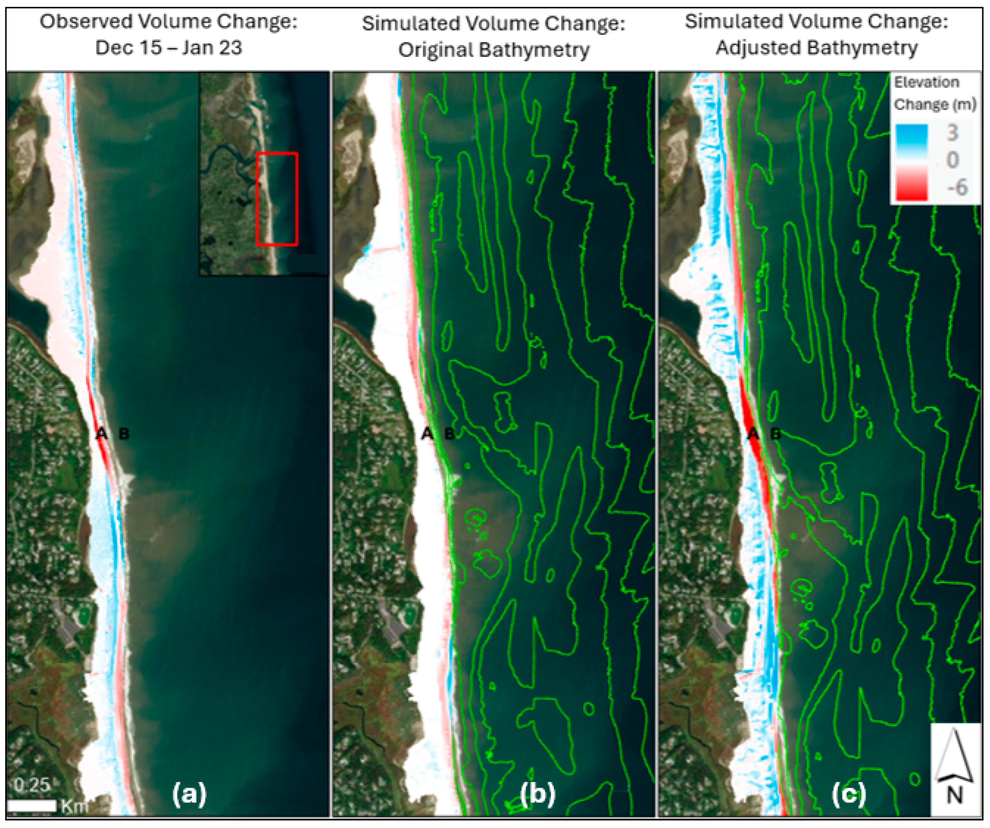
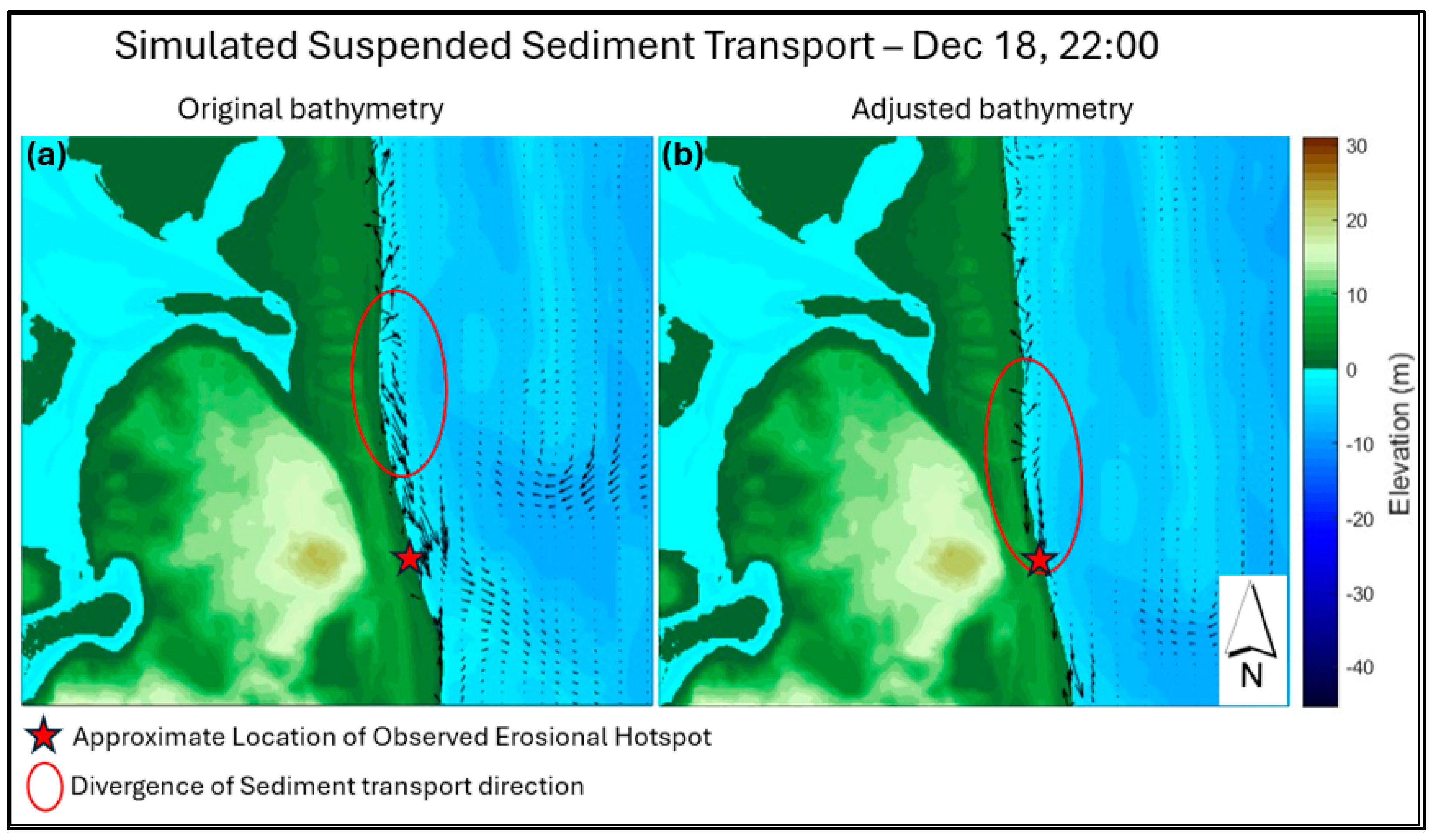
  • Results from XBeach modeling indicated that the location of the erosional hotspot between December and January was largely influenced by the nearshore sandbar configuration. The model scenarios demonstrated how a break in the sandbar increased wave energy and sediment flux near the section of beach that was most severely eroded, and wave direction could not account for the southerly displacement of the erosion hotspot. Dune erosion was augmented in an area with a narrower beach face, which was also likely driven by the influence of the nearshore bathymetry on wave energy and sediment transport.
  • Modeling results indicated that with 0.3 m (1 ft) of SLR, the study area would experience increased erosion during storms as well as more frequent overwash and inundation events. As dune overtopping and breaching become more common in response to higher sea levels, consecutive storms, even of moderate intensity, pose a significant risk of breaching and inlet formation. This research can be used to inform local management as well as dynamics of barrier systems globally.

Author Contributions

Conceptualization, D.J.H., J.P.W., A.R.G., P.S., P.R. and I.G.; methodology, D.J.H., J.P.W., A.R.G., I.G., D.C., S.T.G., C.D. and R.D.; writing—original draft preparation, D.J.H.; writing—review and editing, D.J.H., J.P.W., A.R.G., I.G., S.T.G. and D.C.; visualization, D.J.H., J.P.W., C.D. and R.D.; supervision, J.P.W. and A.R.G.; project administration, J.P.W. and I.G.; discussion, collaboration and communication, All authors; funding acquisition, All authors. All authors have read and agreed to the published version of the manuscript.

Funding

This research was funded by the National Oceanic and Atmospheric Administration, grant number NA21NOS4780149.

Data Availability Statement

Historical data are available from federal sources; details are provided in the text, and data can be downloaded from the NOAA Data Access Viewer: https://coast.noaa.gov/dataviewer (accessed on 19 December 2024). More details and data from the research can be found in Harrington (2024) M.S. Thesis published by the University of Rhode Island after a two-year embargo. Newly collected data and model input and results will be provided through and/or public access will be available to the project hub at the conclusion of project funding in 2026: https://noaa-eslr-edc.hub.arcgis.com/ (accessed on 19 December 2024).

Acknowledgments

Staff from the National Park Service, especially our collaborators Amanda Babson and Monique Lafrance, and others from the Cape Cod National Seashore, provided invaluable support. The Town of Orleans is acknowledged for giving access to their coast and providing insight into and interest in the project, and more specifically, Nathan Sears and Keegan Burke provided direct assistance. Administrative support at the URI Graduate School of Oceanography and the Coastal Resources Center has been critical to the success of this project.

Conflicts of Interest

The authors declare no conflicts of interest.

Appendix A

XBeach Model Calibration

For calibration of the XBeach model, cumulative effects of the 18 December and 7–14 January storms were compared to subaerial elevation changes measured between 15 December and 23 January. Simulations were run with varying combinations of the γua and β parameters, and the γua and β values that produced the best agreement with the observations were used in all subsequent simulations. The performance of these simulations was assessed based on (a) a visual inspection of the subaerial erosion patterns, (b) average eroded volume, and (c) a skill score based on how well the simulation predicted the spatial distribution of the occurrence of erosion.
For the visual inspection of each simulation’s erosion/accretion patterns, after the completion of each simulation, the bed elevation at the final timestep of the model was extracted and converted into an ASCII file and imported in ArcGIS pro. The pre-storm bed-elevation was then subtracted from the final timestep elevations using the Minus tool to create a raster dataset of simulated bed elevation changes. This raster was then clipped to the extent of the drone-surveyed area using the Extract by Mask tool. Maps of both observed and simulated elevation changes were then visualized in ArcGIS Pro (see Figure 9), and major similarities/differences in the patterns of accretion/erosion were noted.
To calculate average eroded volume (ΔV), first the elevation change (Δz) was calculated for each cell in the output dataset by subtracting pre-storm elevations from post-storm elevations on a cell-by-cell basis, so that within each cell of the resulting raster, positive values represent accretion, and negative values represent erosion (Equation (A1)). Equation (A2) was then applied to calculate average eroded volume by multiplying each cell by its x and y dimensions, taking the sum of all the cells, then dividing the result by the length of the section of the beach considered (in this case Lshore = 3675 m). This provides the volume change of the beach in cubic meters per longshore meter of beach (m3/m).
Δz = zfinal − zinitial
ΔV= 1/Lshore ∑n(Δxi · Δyi · Δzi)
A skill score of the spatial distribution of erosion (denoted in this paper as ESS) was used to assess the accuracy of the simulated spatial erosion patterns of each calibration scenario. This skill score is a measure of how many times a simulation agreed with observed data on a binary metric of whether erosion occurred within a particular cell. To calculate this, the simulated and observed elevation change raster datasets were interpolated in MATLAB R2022a to uniform grids of the same size and resolution. Each cell in each grid was then assigned a binary value where 0 represents no erosion and 1 represents erosion. For this classification, Δz ≤ −0.2 m was classified as erosive (b = 1) and cells with Δz > −0.2 m were considered non-erosive (b = 0). This buffer threshold of 0.2 m was included to account for potential inaccuracies in the elevation data resulting from a combination of: (a) inaccuracies in the elevation measurements of the input datasets, (b) interpolation errors which may have occurred when the input raster was interpolated into a varying grid then re-interpolated back to a uniform grid after the simulation, or (c) natural processes that affected the beach during the time periods not included in the simulations. As shown in Equation (A3), a skill score of the spatial distribution of erosion was then obtained by subtracting the binary value from each cell in the measured grid from the corresponding cell in the simulation output grid, then taking the average of the absolute value of those results and subtracting that value from 1. An ESS of one therefore indicates perfect agreement in the locations of erosion between the model and observations while a score of zero indicates total disagreement with the observations. Note that this metric does not consider the magnitude of erosion within each cell, just whether erosion occurred.
E S S = 1 ( 1 n n b s i m , i b m e a s , i )
Table A1. Table of XBeach Calibration results. Simulations with ΔV closer to the measured value of −22.28 and skill scores closer to 1 performed better. γua and β values of 0.24 and 0.07, respectively (simulation 13), resulted in the best agreement with observations.
Simulation #Facua (γua)Beta (β)ΔV (m3/m)ESS
10.240.06−29.880.702
20.240.07−24.060.708
30.240.08−14.750.714
40.220.07−29.520.704
50.220.1−25.080.711

Appendix B

Appendix B.1. Grain Size Distributions

Table A2. Summary grain-size statistics from each survey date.
Collection DateMean D10 (µm)Mean D50 (µm)Mean D90 (µm)
6 September 2023553.2954.81719.3
15 December 2023 *436.2703.71209.3
23 January 2024443.3713.81188.4
14 March 2024486.0833.31505.8
Notes: * Samples from transect 3 on this date were collected ~200m north of the transect 3 location of all other collection dates.
Table A3. Grain-size distributions from each transect collected in December. Note that grain-sizes from within the erosional hotspot were not significantly different than samples taken at other locations alongshore on the same date.
Transect #Mean D10 (µm)Mean D50 (µm)Mean D90 (µm)
1 (Overwash fan)452.0784.71479.4
2 (Overwash fan)424.4684.51185.4
3 (Hotspot)443.2693.11140.7
4 (South of Hotspot)424.4637.2970.1
Figure A1. Map of sediment sampling locations. Numbers indicate the transect number along which samples were collected. Note that samples for Transect 3 in December were collected about 200 m north of the usual Transect 3 location.
Water 17 00245 g0a1

Appendix B.2. Additional Figures

Figure A2. Subaerial volume change between each historical LiDAR dataset from 2011–2021. Blue areas represent accretion and red areas represent erosion.
Water 17 00245 g0a2
Figure A3. Simulated elevation change in XBeach simulations with differing wave direction boundary conditions. The location of maximum simulated erosion was roughly the same in all simulations, indicating wave direction was not a significant control on the location of the erosional hotspot.
Water 17 00245 g0a3
Figure A4. Simulated bed elevation and wave height during two XBeach runs of the December (top) and January (bottom) storms. The data displayed are from select points in the erosional hotspot and immediately offshore of the hotspot (see locations of A and B in Figure 14). Graphs on the (left) are from runs using the original bathymetric input grid, graphs on the (right) are from runs using the adjusted bathymetry grid. The black star indicates the model timestep displayed in Figure 15.
Water 17 00245 g0a4

References

  1. McGranahan, G.; Balk, D.; Anderson, B. The Rising Tide: Assessing the Risks of Climate Change and Human Settlements in Low Elevation Coastal Zones. Environ. Urban. 2007, 19, 17–37. [Google Scholar] [CrossRef]
  2. Crossett, K.; Ache, B.; Pacheco, P.; Haber, K. National Coastal Population Report Population Trends from 1970 to 2020. NOAA’s State of the Coast. 2013. Available online: https://aambpublicoceanservice.blob.core.windows.net/oceanserviceprod/facts/coastal-population-report.pdf (accessed on 14 July 2024).
  3. Church, J.A.; White, N.J. Sea-Level Rise from the Late 19th to the Early 21st Century. Surv. Geophys. 2011, 32, 585–602. [Google Scholar] [CrossRef]
  4. Kopp, R.E.; Kemp, A.C.; Bittermann, K.; Horton, B.P.; Donnelly, J.P.; Gehrels, W.R.; Hay, C.C.; Mitrovica, J.X.; Morrow, E.D.; Rahmstorf, S. Temperature-Driven Global Sea-Level Variability in the Common Era. Proc. Natl. Acad. Sci. USA 2016, 113, 1434–1441. [Google Scholar] [CrossRef] [PubMed]
  5. Sweet, W.V.; Hamlington, B.D.; Kopp, R.E.; Weaver, C.P.; Barnard, P.L.; Bekaert, D.; Brooks, W.; Craghan, M.; Dusek, G.; Frederikse, T.; et al. Global and Regional Sea Level Rise Scenarios for the United States: Updated Mean Projections and Extreme Water Level Probabilities Along U.S. Coastlines; NOAA Technical Report NOS 01; National Oceanic and Atmospheric Administration, National Ocean Service: Silver Spring, MD, USA, 2022. [Google Scholar]
  6. FitzGerald, D.M.; Fenster, M.S.; Argow, B.A.; Buynevich, I.V. Coastal Impacts Due to Sea-Level Rise. Annu. Rev. Earth Planet. Sci. 2008, 36, 601–647. [Google Scholar] [CrossRef]
  7. Goslin, J.; Clemmensen, L.B. Proxy Records of Holocene Storm Events in Coastal Barrier Systems: Storm-Wave Induced Markers. Quat. Sci. Rev. 2017, 174, 80–119. [Google Scholar] [CrossRef]
  8. Otvos, E.G. Coastal Barriers-Fresh Look at Origins, Nomenclature and Classification Issues. Geomorphology 2020, 355, 107000. [Google Scholar] [CrossRef]
  9. Luijendijk, A.; Hagenaars, G.; Ranasinghe, R.; Baart, F.; Donchyts, G.; Aarninkhof, S. The State of the World’s Beaches. Sci. Rep. 2018, 8, 6641. [Google Scholar] [CrossRef] [PubMed]
  10. Pilkey, O.H.; Cooper, J.A.G.; Lewis, D.A. Global Distribution and Geomorphology of Fetch-Limited Barrier Islands. J. Coast. Res. 2009, 254, 819–837. [Google Scholar] [CrossRef]
  11. Elliff, C.I.; Kikuchi, R.K.P. The Ecosystem Service Approach and Its Application as a Tool for Integrated Coastal Management. Nat. Conserv. 2015, 13, 105–111. [Google Scholar] [CrossRef]
  12. Millennium Ecosystem Assessment (Program) (Ed.) Ecosystems and Human Well-Being: Wetlands and Water Synthesis: A Report of the Millennium Ecosystem Assessment; World Resources Institute: Washington, DC, USA, 2005; ISBN 978-1-56973-597-8. [Google Scholar]
  13. Barbier, E.B.; Hacker, S.D.; Kennedy, C.; Koch, E.W.; Stier, A.C.; Silliman, B.R. The Value of Estuarine and Coastal Ecosystem Services. Ecol. Monogr. 2011, 81, 169–193. [Google Scholar] [CrossRef]
  14. Kildow, J.T.; Colgan, C.S.; Johnson, P.; Scorse, J.D.; Farnum, M.G. State of the U.S. Ocean and Coastal Economies—2016 Update; Middlebury Institute of International Studies at Monterey: Monterey, CA, USA, 2016; p. 31. [Google Scholar]
  15. Pilkey, O.H.; Cooper, J.A.G. Are Natural Beaches Facing Extinction? J. Coast. Res. 2014, 70, 431–436. [Google Scholar] [CrossRef]
  16. Rogers, L.J.; Moore, L.J.; Goldstein, E.B.; Hein, C.J.; Lorenzo-Trueba, J.; Ashton, A.D. Anthropogenic Controls on Overwash Deposition: Evidence and Consequences. J. Geophys. Res. Earth Surf. 2015, 120, 2609–2624. [Google Scholar] [CrossRef]
  17. Leatherman, S.P. Barrier Dune Systems: A Reassessment. Sediment. Geol. 1979, 24, 1–16. [Google Scholar] [CrossRef]
  18. Sallenger, A.H. Storm Impact Scale for Barrier Islands. J. Coast. Res. 2000, 16, 7. [Google Scholar]
  19. Masselink, G.; Van Heteren, S. Response of Wave-Dominated and Mixed-Energy Barriers to Storms. Mar. Geol. 2014, 352, 321–347. [Google Scholar] [CrossRef]
  20. Lorenzo-Trueba, J.; Ashton, A.D. Rollover, Drowning, and Discontinuous Retreat: Distinct Modes of Barrier Response to Sea-level Rise Arising from a Simple Morphodynamic Model. JGR Earth Surf. 2014, 119, 779–801. [Google Scholar] [CrossRef]
  21. Passeri, D.L.; Dalyander, P.S.; Long, J.W.; Mickey, R.C.; Jenkins, R.L.; Thompson, D.M.; Plant, N.G.; Godsey, E.S.; Gonzalez, V.M. The Roles of Storminess and Sea Level Rise in Decadal Barrier Island Evolution. Geophys. Res. Lett. 2020, 47, e2020GL089370. [Google Scholar] [CrossRef]
  22. Conery, I.; Walsh, J.P.; Reide Corbett, D. Hurricane Overwash and Decadal-Scale Evolution of a Narrowing Barrier Island, Ocracoke Island, NC. Estuaries Coasts 2018, 41, 1626–1642. [Google Scholar] [CrossRef]
  23. Donnelly, C.; Kraus, N.C.; Larson, M. Coastal Overwash: Part 1, Overview of Processes. 2004. Available online: https://apps.dtic.mil/sti/tr/pdf/ADA602107.pdf (accessed on 14 July 2024).
  24. Kraus, N.C.; Militello, A.; Todoroff, G. Barrier Breaching Processes and Barrier Spit Breach, Stone Lagoon, California. 2002. Available online: https://apps.dtic.mil/sti/tr/pdf/ADA483417.pdf (accessed on 14 July 2024).
  25. McCall, R.T.; Van Thiel De Vries, J.S.M.; Plant, N.G.; Van Dongeren, A.R.; Roelvink, J.A.; Thompson, D.M.; Reniers, A.J.H.M. Two-Dimensional Time Dependent Hurricane Overwash and Erosion Modeling at Santa Rosa Island. Coast. Eng. 2010, 57, 668–683. [Google Scholar] [CrossRef]
  26. McCall, R.; Masselink, G.; Poate, T.; Bradbury, A.; Russell, P.; Davidson, M. Predicting Overwash on Gravel Barriers. J. Coast. Res. 2013, 165, 1473–1478. [Google Scholar] [CrossRef]
  27. Plomaritis, T.A.; Ferreira, Ó.; Costas, S. Regional Assessment of Storm Related Overwash and Breaching Hazards on Coastal Barriers. Coast. Eng. 2018, 134, 124–133. [Google Scholar] [CrossRef]
  28. Roelvink, D.; Reniers, A.; Van Dongeren, A.; Van Thiel De Vries, J.; McCall, R.; Lescinski, J. Modelling Storm Impacts on Beaches, Dunes and Barrier Islands. Coast. Eng. 2009, 56, 1133–1152. [Google Scholar] [CrossRef]
  29. Stockdon, H.F.; Sallenger, A.H.; Holman, R.A.; Howd, P.A. A Simple Model for the Spatially-Variable Coastal Response to Hurricanes. Mar. Geol. 2007, 238, 1–20. [Google Scholar] [CrossRef]
  30. Schambach, L.; Grilli, A.R.; Grilli, S.T.; Hashemi, M.R.; King, J.W. Assessing the Impact of Extreme Storms on Barrier Beaches along the Atlantic Coastline: Application to the Southern Rhode Island Coast. Coast. Eng. 2018, 133, 26–42. [Google Scholar] [CrossRef]
  31. Schuh, E.; Grilli, A.R.; Groetsch, F.; Grilli, S.T.; Crowley, D.; Ginis, I.; Stempel, P. Assessing the morphodynamic response of a New England beach-barrier system to an artificial reef. Coast. Eng. 2023, 184, 104355. [Google Scholar] [CrossRef]
  32. Grilli, A.R.; Westcott, G.; Grilli, S.; Spaulding, M.L.; Shi, F. and J.T. Kirby. Assessing coastal risk from extreme storms with a phase resolving wave model: Case Study of Narragansett, RI, USA. Coast. Eng. 2020, 160, 103735. [Google Scholar] [CrossRef]
  33. Grilli, A.R.; Spaulding, M.L.; Oakley, B.A.; Damon, C. Mapping the coastal risk for the next century, including sea level rise and changes in the coastline: Application to Charlestown RI, USA. Nat. Hazards 2017, 88, 389–414. [Google Scholar] [CrossRef]
  34. Kraus, N.C.; Galgano, F.A. Beach Erosional Hot Spots: Types, Causes, and Solutions. 2001. Available online: https://apps.dtic.mil/sti/tr/pdf/ADA588792.pdf (accessed on 14 July 2024).
  35. McNinch, J.E. Geologic Control in the Nearshore: Shore-Oblique Sandbars and Shoreline Erosional Hotspots, Mid-Atlantic Bight, USA. Mar. Geol. 2004, 211, 121–141. [Google Scholar] [CrossRef]
  36. Mulligan, R.P.; Gomes, E.R.; Miselis, J.L.; McNinch, J.E. Non-Hydrostatic Numerical Modelling of Nearshore Wave Transformation over Shore-Oblique Sandbars. Estuar. Coast. Shelf Sci. 2019, 219, 151–160. [Google Scholar] [CrossRef]
  37. Stive, M.J.F.; Guillen, J.; Capobianco, M. Bar Migration and Duneface Oscillation on Decadal Scales. In Proceedings of the Coastal Engineering 1996; American Society of Civil Engineers: Orlando, FL, USA, 1997; pp. 2884–2896. [Google Scholar]
  38. List, J.H.; Farris, A.S.; Sullivan, C. Reversing Storm Hotspots on Sandy Beaches: Spatial and Temporal Characteristics. Mar. Geol. 2006, 226, 261–279. [Google Scholar] [CrossRef]
  39. Joyce, K.E.; Belliss, S.E.; Samsonov, S.V.; McNeill, S.J.; Glassey, P.J. A Review of the Status of Satellite Remote Sensing and Image Processing Techniques for Mapping Natural Hazards and Disasters. Prog. Phys. Geogr. Earth Environ. 2009, 33, 183–207. [Google Scholar] [CrossRef]
  40. Moore, L.J. Shoreline Mapping Techniques. J. Coast. Res. 2024, 16, 111–124. [Google Scholar]
  41. Giordan, D.; Manconi, A.; Remondino, F.; Nex, F. Use of Unmanned Aerial Vehicles in Monitoring Application and Management of Natural Hazards. Geomat. Nat. Hazards Risk 2017, 8, 1–4. [Google Scholar] [CrossRef]
  42. Caroti, G.; Piemonte, A.; Pieracci, Y. Low-Altitude UAV-Borne Remote Sensing in Dunes Environment: Shoreline Monitoring and Coastal Resilience. In Computational Science and Its Applications–ICCSA 2018; Gervasi, O., Murgante, B., Misra, S., Stankova, E., Torre, C.M., Rocha, A.M.A.C., Taniar, D., Apduhan, B.O., Tarantino, E., Ryu, Y., Eds.; Lecture Notes in Computer Science; Springer International Publishing: Cham, Switzerland, 2018; Volume 10964, pp. 281–293. ISBN 978-3-319-95173-7. [Google Scholar]
  43. Westoby, M.J.; Brasington, J.; Glasser, N.F.; Hambrey, M.J.; Reynolds, J.M. ‘Structure-from-Motion’ Photogrammetry: A Low-Cost, Effective Tool for Geoscience Applications. Geomorphology 2012, 179, 300–314. [Google Scholar] [CrossRef]
  44. Mancini, F.; Dubbini, M.; Gattelli, M.; Stecchi, F.; Fabbri, S.; Gabbianelli, G. Using Unmanned Aerial Vehicles (UAV) for High-Resolution Reconstruction of Topography: The Structure from Motion Approach on Coastal Environments. Remote Sens. 2013, 5, 6880–6898. [Google Scholar] [CrossRef]
  45. Beckman, J.N.; Long, J.W.; Hawkes, A.D.; Leonard, L.A.; Ghoneim, E. Investigating Controls on Barrier Island Overwash and Evolution during Extreme Storms. Water 2021, 13, 2829. [Google Scholar] [CrossRef]
  46. Nederhoff, K.; Lodder, Q.; Boers, M.; Bieman, J.; Miller, J. Modelling the Effects of Hard Structures on Dune Erosion and Overwash-a Case Study of the Impact of Hurricane Sandy on the New Jersey Coast. 2015. Available online: https://www.researchgate.net/publication/311934611_Modeling_the_effects_of_hard_structures_on_dune_erosion_and_overwash (accessed on 14 July 2024).
  47. Giese, G.S.; Borrelli, M.; Mague, S.T. Tidal Inlet Evolution and Impacts of Anthropogenic Alteration: An Example from Nauset Beach and Pleasant Bay, Cape Cod, Massachusetts. Northeast. Nat. 2020, 27, 1. [Google Scholar] [CrossRef]
  48. Borrelli, M.; Boothroyd, J.C. Calculating Rates of Shoreline Change in a Coastal Embayment with Fringing Salt Marsh Using the “Marshline”, a Proxy-Based Shoreline Indicator. Northeast. Nat. 2020, 27, 132. [Google Scholar] [CrossRef]
  49. Redfield, A.C. Ontogeny of a Salt Marsh Estuary. Science 1965, 147, 50–55. [Google Scholar] [CrossRef] [PubMed]
  50. Redfield, A.C. Development of a New England Salt Marsh. Ecol. Monogr. 1972, 42, 201–237. [Google Scholar] [CrossRef]
  51. Data Cape Cod. Available online: https://datacapecod.org/pf/barnstable-county-year-round-population/ (accessed on 14 July 2024).
  52. Hotchkiss, E.; Kandt, A.; Holm, A.; McKean, L.; Norton, S. Resilience Assessment: Cape Cod National Seashore; NREL/TP-7A40-79171; National Renewable Energy Laboratory: Golden, CO, USA, 2021. [Google Scholar]
  53. Borrelli, M.; Giese, G.; Mague, S.T.; Smith, T.; Mittermayr, A.; Legare, B.J.; Solazzo, D. Potential Impacts to the Nau-set Barrier from the Proposed Dredging and Disposal in Nauset Harbor; Coastal Processes and Ecosystems Laboratory, Center for Coastal Studies: Provincetown, MA, USA, 2019. [Google Scholar] [CrossRef]
  54. Giese, G.S.; Adams, M.B.; Rogers, S.S.; Lawrence Dingman, S.; Borrelli, M.; Smith, T.L. Coastal Sediment Transport on Outer Cape Cod, Massachusetts: Observation And Theory. In The Proceedings of the Coastal Sediments 2011; World Scientific Publishing Company: Miami, Florida, USA, 2011; pp. 2353–2365. [Google Scholar]
  55. Bartlett, M.K.; Henderson, R.E.; Farris, A.; Himmelstoss, E. Massachusetts Shoreline Change Project, 2021 Update: A GIS Compilation of Shoreline Change Rates Calculated Using Digital Shoreline Analysis System Version 5.1, With Supplementary Intersects and Baselines for Massachusetts; Woods Hole Coastal and Marine Science Center: Woods Hole, MA, USA, 2021. [Google Scholar]
  56. Aubrey, D.G.; Speer, P.E. Updrift Migration of Tidal Inlets. J. Geol. 1984, 92, 531–545. [Google Scholar] [CrossRef]
  57. Woods Hole Group. Nauset Estuary Dredging Feasibility Assessment; Prepared for the town of Orleans by Woods Hole Group. 2016. Available online: https://town.orleans.ma.us/DocumentCenter/View/6533/Nauset-Estuary-Dredging-Feasibility-Assessment---WHG-Feb-2016 (accessed on 14 July 2024).
  58. NOAA: Data Access Viewer. Available online: https://coast.noaa.gov/dataviewer/#/lidar/search/ (accessed on 5 September 2024).
  59. Pix4D Documentation|PIX4Dmapper. Available online: https://support.pix4d.com/hc/pix4dmapper#manual (accessed on 5 September 2024).
  60. National Geodetic Survey, 2024: 2022 NOAA NGS Topobathy Lidar: Chatham Bay to Monomoy Point, MA. Available online: https://coast.noaa.gov/dataviewer/#/lidar/search/-7804526.336029637,5124338.376238216,-7778598.881106198,5153200.977591176 (accessed on 14 July 2024).
  61. OCM Partners, 2024: 2021 USGS Lidar: Central Eastern Massachusetts. Available online: https://coast.noaa.gov/dataviewer/#/lidar/search/-7804526.336029637,5124338.376238216,-7778598.881106198,5153200.977591176 (accessed on 14 July 2024).
  62. OCM Partners, 2024: 2018 USACE NCMP Topobathy LiDAR DEM: East Coast (CT, MA, ME, NC, NH, RI, SC). Available online: https://coast.noaa.gov/dataviewer/#/lidar/search/-7804526.336029637,5124338.376238216,-7778598.881106198,5153200.977591176 (accessed on 14 July 2024).
  63. OCM Partners, 2024: 1887–2016 USGS CoNED Topobathy DEM (Compiled 2016): New England. Available online: https://coast.noaa.gov/dataviewer/#/lidar/search/-7804526.336029637,5124338.376238216,-7778598.881106198,5153200.977591176 (accessed on 14 July 2024).
  64. Office for Coastal Management, 2024: 2020–2023 CCAP Version 2 Impervious Cover. Available online: https://coast.noaa.gov/dataviewer/#/landcover/search/-7791837.789334295,5123421.131898793,-7780708.559882113,5138830.834934946 (accessed on 14 July 2024).
  65. Office for Coastal Management, 2024: C-CAP Land Cover, Massachusetts. 2016. Available online: https://coast.noaa.gov/dataviewer/#/landcover/search/-7791837.789334295,5123421.131898793,-7780708.559882113,5138830.834934946 (accessed on 14 July 2024).
  66. Dietrich, J.C.; Westerink, J.J.; Kennedy, A.B.; Smith, J.M.; Jensen, R.E.; Zijlema, M.; Holthuijsen, L.H.; Dawson, C.; Luettich, R.A.; Powell, M.D.; et al. Hurricane Gustav (2008) Waves and Storm Surge: Hindcast, Synoptic Analysis, and Validation in Southern Louisiana. Mon. Weather Rev. 2011, 139, 2488–2522. [Google Scholar] [CrossRef]
  67. Dee, D.P.; Uppala, S.M.; Simmons, A.J.; Berrisford, P.; Poli, P.; Kobayashi, S.; Andrae, U.; Balmaseda, M.A.; Balsamo, G.; Bauer, P.; et al. The ERA-Interim Reanalysis: Configuration and Performance of the Data Assimilation System. Q. J. R. Meteorol. Soc. 2011, 137, 553–597. [Google Scholar] [CrossRef]
  68. National Weather Service Coastal Storm: December 17–18, 2023. Available online: https://www.weather.gov/ilm/Dec2023CoastalStorm (accessed on 16 July 2024).
  69. National Data Buoy Center Buoy Data from Station 44018. Available online: https://www.ndbc.noaa.gov/station_history.php?station=44018 (accessed on 16 July 2024).
  70. January 2024 National Climate Report | National Centers for Environmental Information (NCEI). Available online: https://www.ncei.noaa.gov/access/monitoring/monthly-report/national/202401 (accessed on 16 July 2024).
  71. Zhang, K.; Douglas, B.C.; Leatherman, S.P. Twentieth-Century Storm Activity along the U.S. East Coast. J. Clim. 2000, 13, 1748–1761. [Google Scholar] [CrossRef]
  72. Ostiguy, L.J.; Sargent, T.C.; Izbicki, B.J.; Bent, G.C. High-Water Marks from Hurricane Sandy for Coastal Areas of Connecticut, Rhode Island, and Massachusetts, October 2012; U.S. Geological Survey Data Series 1094; U.S. Geological Survey: Reston, VA, USA, 2018; 16p. [Google Scholar] [CrossRef]
  73. Massey, A.J.; Verdi, R.J. Storm Tide Monitoring During the Blizzard of January 26–28, 2015, in Eastern Massachusetts; U.S. Geological Survey: Reston, VA, USA, 2015. [Google Scholar]
  74. Bent, G.C.; Taylor, N.J. Total Water Level Data from the January and March 2018 Nor’easters for Coastal Areas of New England; Open-File Report 2020–5048; U.S. Geological Survey Scientific Investigations Report: Reston, VA, USA, 2022; 47p. [Google Scholar] [CrossRef]
  75. Birchler, J.J.; Stockdon, H.F.; Doran, K.S.; Thompson, D.M. National Assessment of Hurricane-Induced Coastal Erosion Hazards—Northeast Atlantic Coast; Open-File Report 2014–1243; U.S. Geological Survey: Reston, VA, USA, 2014; 34p. [Google Scholar] [CrossRef]
  76. Global Catastrophe Recap-May 2018. Available online: https://www.actuarialpost.co.uk/downloads/cat_1/Aon-ab-analytics-if-may-global-recap.pdf (accessed on 16 July 2024).
  77. Bullard, J.E.; Ackerley, D.; Millett, J.; Chandler, J.H.; Montreuil, A.-L. Post-Storm Geomorphic Recovery and Resilience of a Prograding Coastal Dune System. Environ. Res. Commun. 2019, 1, 011004. [Google Scholar] [CrossRef]
  78. Leatherman, S.P.; Zaremba, R.E. Overwash and Aeolian Processes on A U.S. Northeast Coast Barrier. Sediment. Geol. 1987, 52, 183–206. [Google Scholar] [CrossRef]
  79. Castelle, B.; Bujan, S.; Ferreira, S.; Dodet, G. Foredune Morphological Changes and Beach Recovery from the Extreme 2013/2014 Winter at a High-Energy Sandy Coast. Mar. Geol. 2017, 385, 41–55. [Google Scholar] [CrossRef]
  80. Houser, C.; Wernette, P.; Rentschlar, E.; Jones, H.; Hammond, B.; Trimble, S. Post-Storm Beach and Dune Recovery: Implications for Barrier Island Resilience. Geomorphology 2015, 234, 54–63. [Google Scholar] [CrossRef]
  81. USGS Open-File Report 2010-1118: National Assessment of Shoreline Change: Historical Shoreline Change Along the New England and Mid-Atlantic Coasts. Available online: https://pubs.usgs.gov/of/2010/1118/ (accessed on 11 September 2024).
  82. Heaslip, S. Saturday Storm Brings Rain, Wind and Coastal Flooding to Cape Cod. Available online: https://www.capecodtimes.com/picture-gallery/news/2024/01/13/third-storm-of-the-week-brings-rainwind-and-flooding-to-cape-cod/72216811007/ (accessed on 11 September 2024).
  83. McCarron, H. Cape Cod, Nantucket Clock State’s Highest Wind Gusts in Storm. Thousands Without Power. Available online: https://www.capecodtimes.com/story/weather/2023/12/18/cape-cod-wind-storm-eversource-power-outages-rain-weather/71963474007/ (accessed on 11 September 2024).
  84. Cohn, N.; Brodie, K.L.; Johnson, B.; Palmsten, M.L. Hotspot Dune Erosion on an Intermediate Beach. Coast. Eng. 2021, 170, 103998. [Google Scholar] [CrossRef]
  85. Schupp, C.A.; McNinch, J.E.; List, J.H. Nearshore Shore-Oblique Bars, Gravel Outcrops, and Their Correlation to Shoreline Change. Mar. Geol. 2006, 233, 63–79. [Google Scholar] [CrossRef]
  86. Gallagher, E.L.; MacMahan, J.; Reniers, A.J.H.M.; Brown, J.; Thornton, E.B. Grain Size Variability on a Rip-Channeled Beach. Mar. Geol. 2011, 287, 43–53. [Google Scholar] [CrossRef]
  87. Stive, M.J.F.; Aarninkhof, S.G.J.; Hamm, L.; Hanson, H.; Larson, M.; Wijnberg, K.M.; Nicholls, R.J.; Capobianco, M. Variability of Shore and Shoreline Evolution. Coast. Eng. 2002, 47, 211–235. [Google Scholar] [CrossRef]
  88. Maa, J.P.-Y.; Hobbs, C.H. Physical Impact of Waves on Adjacent Coasts Resulting from Dredging at Sand-bridge Shoal, Virginia. J. Coast. Res. 1998, 14, 525–536. [Google Scholar]
  89. Cheng, J.; Wang, P. Factors Controlling Storm-Induced Morphology Changes at an Erosional Hot Spot on a Nourished Beach, Sand Key Barrier Island, West-Central Florida. J. Coast. Res. 2022, 38, 750–765. [Google Scholar] [CrossRef]
  90. Richmond, B.M.; Sallenger, A.H. Cross-Shore Transport of Bimodal Sands. In Proceedings of the Nineteenth Coastal Engineering Conference, Houston, TX, USA, 3–7 September 1984; ASCE: New York, NY, USA, 1985. [Google Scholar]
  91. Harrington, D.J. Past and Future Storm-Driven Changes to a Dynamic Sandy Barrier System: Outer Cape Cod, MA. Master’s Thesis, University of Rhode Island, Kingston, RI, USA, 2024. [Google Scholar]
  92. Gao, J. Bathymetric Mapping by Means of Remote Sensing: Methods, Accuracy and Limitations. Prog. Phys. Geogr. Earth Environ. 2009, 33, 103–116. [Google Scholar] [CrossRef]
  93. Dugan, J.P.; Morris, W.D.; Vierra, K.C.; Piotrowski, C.C.; Farruggia, G.J. Jetski-Based Nearshore Bathymetric and Current Survey System. J. Coast. Res. 2001, 17, 900–908. [Google Scholar]
  94. Kimball, P.; Bailey, J.; Das, S.; Geyer, R.; Harrison, T.; Kunz, C.; Manganini, K.; Mankoff, K.; Samuelson, K.; Sayre-McCord, T.; et al. The WHOI Jetyak: An Autonomous Surface Vehicle for Oceanographic Research in Shallow or Dangerous Waters. In Proceedings of the 2014 IEEE/OES Autonomous Underwater Vehicles (AUV), Oxford, MS, USA, 6–9 October 2014. [Google Scholar]
  95. Holman, R.; Haller, M.C. Remote Sensing of the Nearshore. Annu. Rev. Mar. Sci. 2013, 5, 95–113. [Google Scholar] [CrossRef] [PubMed]
  96. Bergsma, E.W.J.; Almar, R. Video-Based Depth Inversion Techniques, a Method Comparison with Synthetic Cases. Coast. Eng. 2018, 138, 199–209. [Google Scholar] [CrossRef]
  97. Lange, A.M.Z.; Fiedler, J.W.; Merrifield, M.A.; Guza, R.T. UAV Video-Based Estimates of Nearshore Bathymetry. Coast. Eng. 2023, 185, 104375. [Google Scholar] [CrossRef]
  98. Almar, R.; Bergsma, E.W.J.; Brodie, K.L.; Bak, A.S.; Artigues, S.; Lemai-Chenevier, S.; Cesbron, G.; Delvit, J.-M. Coastal Topo-Bathymetry from a Single-Pass Satellite Video: Insights in Space-Videos for Coastal Monitoring at Duck Beach (NC, USA). Remote Sens. 2022, 14, 1529. [Google Scholar] [CrossRef]
  99. Horton, B.P.; Rahmstorf, S.; Engelhart, S.E.; Kemp, A.C. Expert Assessment of Sea-Level Rise by AD 2100 and AD 2300. Quat. Sci. Rev. 2014, 84, 1–6. [Google Scholar] [CrossRef]
  100. D’Anna, M.; Idier, D.; Castelle, B.; Vitousek, S.; Le Cozannet, G. Reinterpreting the Bruun Rule in the Context of Equilibrium Shoreline Models. JMSE 2021, 9, 974. [Google Scholar] [CrossRef]
  101. Gastineau, G.; Soden, B.J. Model Projected Changes of Extreme Wind Events in Response to Global Warming. Geophys. Res. Lett. 2009, 36, L10810. [Google Scholar] [CrossRef]
  102. Stephens, G. Storminess in a Warming World. Nat. Clim Change 2011, 1, 252–253. [Google Scholar] [CrossRef]
  103. De Vet, P.L.M. Modelling Sediment Transport and Morphology during Overwash and Breaching Events. Master’s Thesis, Delft University of Technology, Delft, The Netherlands, 2014. [Google Scholar]
  104. Lee, G.; Nicholls, R.J.; Birkemeier, W.A. Storm-Driven Variability of the Beach-Nearshore Profile at Duck, North Carolina, USA, 1981–1991. Mar. Geol. 1998, 148, 163–177. [Google Scholar] [CrossRef]
  105. Morton, R.A. Factors Controlling Storm Impacts on Coastal Barriers and Beaches: A Preliminary Basis for near Real-Time Forecasting. J. Coast. Res. 2002, 18, 486–501. [Google Scholar]
  106. Fenster, M.S.; Dominguez, R. Quantifying Coastal Storm Impacts Using a New Cumulative Storm Impact Index (CSII) Model: Application Along the Virginia Coast, USA. JGR Earth Surf. 2022, 127, e2022JF006641. [Google Scholar] [CrossRef]
Figure 1. Map of the study region and field mapping area. Nauset Beach is located in the towns of Eastham and Orleans in Outer Cape Cod, MA. The red outline represents the area in which field observations and aerial surveys were conducted.
Water 17 00245 g001
Figure 2. Locations of transects (indicated by the red bars) along which RTK elevation points and sediment samples were collected.
Water 17 00245 g002
Figure 3. Map of data sources for XBeach bathymetric input grid. During calibration, model performance was assessed based on subaerial changes within the purple area, where the most recent pre- and post-storm observations were collected.
Water 17 00245 g003
Figure 4. Water levels (MWL) and significant wave heights time series, at seaward offshore boundary of the modeling domain of the study area, for the 18 December 2023, and 7–14 January 2024 storms. Storm data were extracted from ADCIRC-SWAN models forced by the European Centre for Medium Range Weather Forecasts (ECMWF) reanalysis product ERA5 [67].
Water 17 00245 g004
Figure 5. Aerial imagery of a portion of Nauset Beach from 2011, 2013, 2019, 2021, and 2023. Note, the appearance of an overwash fan in 2019 and subsequent reappearance of dune vegetation in that area in 2021–2023. (Imagery accessed through ArcGIS online from Digital Globe and MassGIS).
Water 17 00245 g005
Figure 6. (Left): Graph of the alongshore variability of volume change corresponding to the map of subaerial elevation change in the study area from 2011–2021. (Right): Elevation transects derived from 2011, 2013/2014, 2018 and 2021 LiDAR datasets at (A) an overwash fan on the spit, and (B) a tall dune. Maps of elevation change between each timestep for this area can be found in Appendix B.
Water 17 00245 g006
Figure 7. (Left) Map of subaerial elevation change in the survey area between 6 September 2023 and 14 March 2024 based on drone mapping. Red areas indicate erosion and blue regions indicate accretion. (Right) Elevation transects at each survey date from (C) the overwash fan, (D) the erosional hotspot, and (E) the area immediately south of the erosional hotspot.
Water 17 00245 g007
Figure 8. Temporal (a) and spatial (b) variation of the grainsize distribution of the sand-sized portion of surface sediments collected withing the survey area between September 2023 and March 2024.
Water 17 00245 g008
Figure 9. (a) Map of subaerial volume changes observed between 15 December 2023 and 23 January 2024. (b) Map of cumulative simulated sediment change for the best-performing calibration simulation of the consecutive XBeach simulations of the 18 December storm and the January cluster of storms. Black lines indicate the locations of the elevation transects in Figure 10.
Water 17 00245 g009
Figure 10. Observed versus simulated post-storm elevation profiles after the December and January storms. Transect locations are displayed in Figure 9. Note that the model overestimated erosion at Transect F (the simulated erosional hotpot), and underestimated change at Transect G (the observed erosional hotspot).
Water 17 00245 g010
Figure 11. Map of maximum inundated area during XBeach simulations of (a) the 18 December storm, (b) the 18 December storm with 1 ft of SLR, and (c) the January storm cluster with 1 ft of SLR.
Water 17 00245 g011
Figure 12. Maps of simulated subaerial volume change with XBeach from (a) the 18 December storm modeled with 1 ft of SLR, and (b) both the 18 December storm and the January storm cluster modeled consecutively with 1 ft of SLR.
Water 17 00245 g012
Figure 13. Spatial distribution of elevation change in the survey area between each survey date in the winter of 2023–2024. Note the area of focused erosion located south of the spit that occurred between December and January. Also notice the accretion that occurred immediately south of the erosional hotspot from September to January, and the reversal of the erosion/accretion trends in both locations from January to March. The background imagery is from 2023 and likely does not reflect the time-varying shoaling and suspended sediment.
Water 17 00245 g013
Figure 14. Maps of observed and simulated subaerial elevation change for 15 December–23 January (a) shows observed changes, (b) shows simulation results using the most recent available bathymetry, and (c) shows simulations results with the bathymetry shifted southward to reflect possible recent sandbar evolution. Points A and B represent the location of the time series of bed elevation and wave height, respectively, in Figure A4.
Water 17 00245 g014
Figure 15. Maps of Sediment transport at 22:00 EST in XBeach simulations of the 18 December storm using (a) original input bathymetry and (b) adjusted bathymetry. The location of the measured erosion hotspot is noted by the red star. Note the southward shift in the location of sediment transport divergence in the simulation with southward shifted bathymetry.
Water 17 00245 g015
Table 1. Table of subaerial volume change per meter of beach length within the study area from 2011 to 2021.
2011–20142014–20182018–20212011–2021
Erosion (m3/m)−86.4−42.6−44.9−86.6
Accretion (m3/m)32.991.937.397.6
Total volume change (m3/m)−53.549.4−7.511.0
Rate of Change (m3/m/yr)−17.812.4−2.51.1
Dune volume change (m3/m)−33.7−6.6−5.1−31.8
Table 2. Subaerial volume change of the study area between 2023 September and March 2024.
Sep–DecDec–JanJan–MarSep–Mar
Erosion (m3/m)−23.4−38.1−34.0−64.2
Accretion (m3/m)13.015.815.919.3
Net Volume Change (m3/m)−10.4−22.3−18.0−44.9
Rate of erosion (m3/m/yr) **−37.8−208.5−129.0−86.2
Volume Change at Hotspot (m3/m) *−57.0−103.816.3−144.5
Notes: * Volume changes at the erosional hotspot are calculated from differences in sediment volume between survey dates at Transect D in Figure 7. ** The rate of erosion was calculated using the fraction of the year for the period analyzed.
Table 3. Averaged D50 grain sizes in µm (of sand portion of samples) for subsets of surface sediment samples collected within particular sections of the survey area between September 2023 and March 2024.
Sample SubsetnOverwashDuneBeach
6 September 202326939.5844.81027.3
15 December 202318783.0633.5680.5
23 January 202419737.6693.3696.2
14 March 202418896.5796.4830.9
All Samples81847.3756.0838.3
Table 4. Sediment volume change statistics observed between 15 December and 23 January and from the combined simulations of the 18 December and 7–14 January storms.
Erosion (m3/m)Accretion (m3/m)Total Change (m3/m)
Observation−38.115.77−22.3
Simulation−26.72.70−24.1
Disclaimer/Publisher’s Note: The statements, opinions and data contained in all publications are solely those of the individual author(s) and contributor(s) and not of MDPI and/or the editor(s). MDPI and/or the editor(s) disclaim responsibility for any injury to people or property resulting from any ideas, methods, instructions or products referred to in the content.

