Spatial Regularities of Changes in the Duration of Low River Flows in Poland Under Climate Warming Conditions

Abstract

On the basis of daily discharges recorded in 140 water gauges located on 96 Polish rivers, the long-term changes of runoff and the number of days with low flows (ND_LF) in relation to selected meteorological variables were studied. The analyses were performed for the entire multi-annual period 1951–2020 and two sub-periods: 1951–1988 and 1988–2020 that are before and after climate change. The average values of these hydro-meteorological variables in the two sub-periods were then compared. It was found that after 1988, a statistically significant (p < 0.001) increase in the average air temperatures, ranging from 0.9 to over 1.3 °C, occurred. Similarly, statistically significant changes were determined for evaporation, which increased by about 10–25%. Precipitation did not show such changes—a statistically significant decrease in precipitation (by over 5%) was recorded only in the southern part of the Odra River basin, and in most stations, statistically insignificant increases were recorded. The most complex changes took place in river runoff. After 1988, in most gauges, a decrease in runoff by about 5–15% was detected; in some cases, these decreases were statistically significant. In the south-eastern part of the country, primarily in the catchments of the right tributaries of the Vistula River, an increase in runoff by about 5–10% was detected. However, only in the case of one gauge, these tendencies were statistically significant. Next, in order to determine spatial regularities in long-term changes in the ND_LF, the cluster analysis method was used, and the gauges were grouped according to the values of 70 annual ND_LF. This resulted in separating three relatively homogenous territorially groups of rivers, demonstrating a clear regional differentiation of ND_LF. It was concluded that separation of these three groups of rivers in terms of different long-term changes in ND_LF was mainly influenced by climatic conditions.

1. Introduction

In the period of progressive global warming, water circulation conditions are changing [1,2,3,4]. This concerns, among others, river regimes, including high- and low-water periods. In Europe, including Poland, this is primarily associated with changes in river water supply conditions [5,6] as a result of changing patterns of evaporation [7] and precipitation distribution in the yearly cycle [8,9], decreasing thickness and duration of snow cover [10], increasing rainfall intensity [11] and changing types of precipitation characteristic of a given season, primarily the occurrence of rain instead of snow in winter [12,13]. Another cause is the rising air temperature and longer and more severe heat waves [14], which increase evaporation and also affect the thermal regime of streams [15,16,17] and lakes [18,19].

In the context of changes in river regimes, both from the point of view of the natural environment and economic activity, hydrological droughts are particularly important, which are manifested by low flows in rivers. Raczyński and Dyer [20], using the trend decomposition method, showed that streamflow droughts were increasing in many parts of Poland, especially in the central, western, and southwestern regions. These results differ from the findings of earlier modeling [21,22], which indicated that future streamflow droughts were projected to be less severe [23]. Wrzesiński et al. [24] indicated that from 1951 to 1988, most of the analyzed gauges showed decreasing trends in the number of days with low flows, but this trend changed and increased from 1988 to 2020. This may be related to the observed climate change in Poland [25], reflected in meteorological data since 1988 [26]. Additionally, the occurrence of low flows on rivers in Poland may be associated with, among others, the temperature of surface waters and thermohaline circulation of the North Atlantic [27,28,29].

Until now, most studies on the hydrology of low flows on Polish rivers have treated the hydrological conditions after 1951 as stationary. While in the latest scientific literature the impact of climate change on river regimes in Poland has been investigated [30,31,32,33,34], there is still a lack of studies on the regional differentiation in the occurrence and course of low flows on Polish rivers.

The aim of this paper is to fill this research gap and present results of research on determining the multi-annual variability and the spatial differentiation in the number of days with low flows (ND_LF) in Polish rivers in the context of the climate warming observed after 1988.

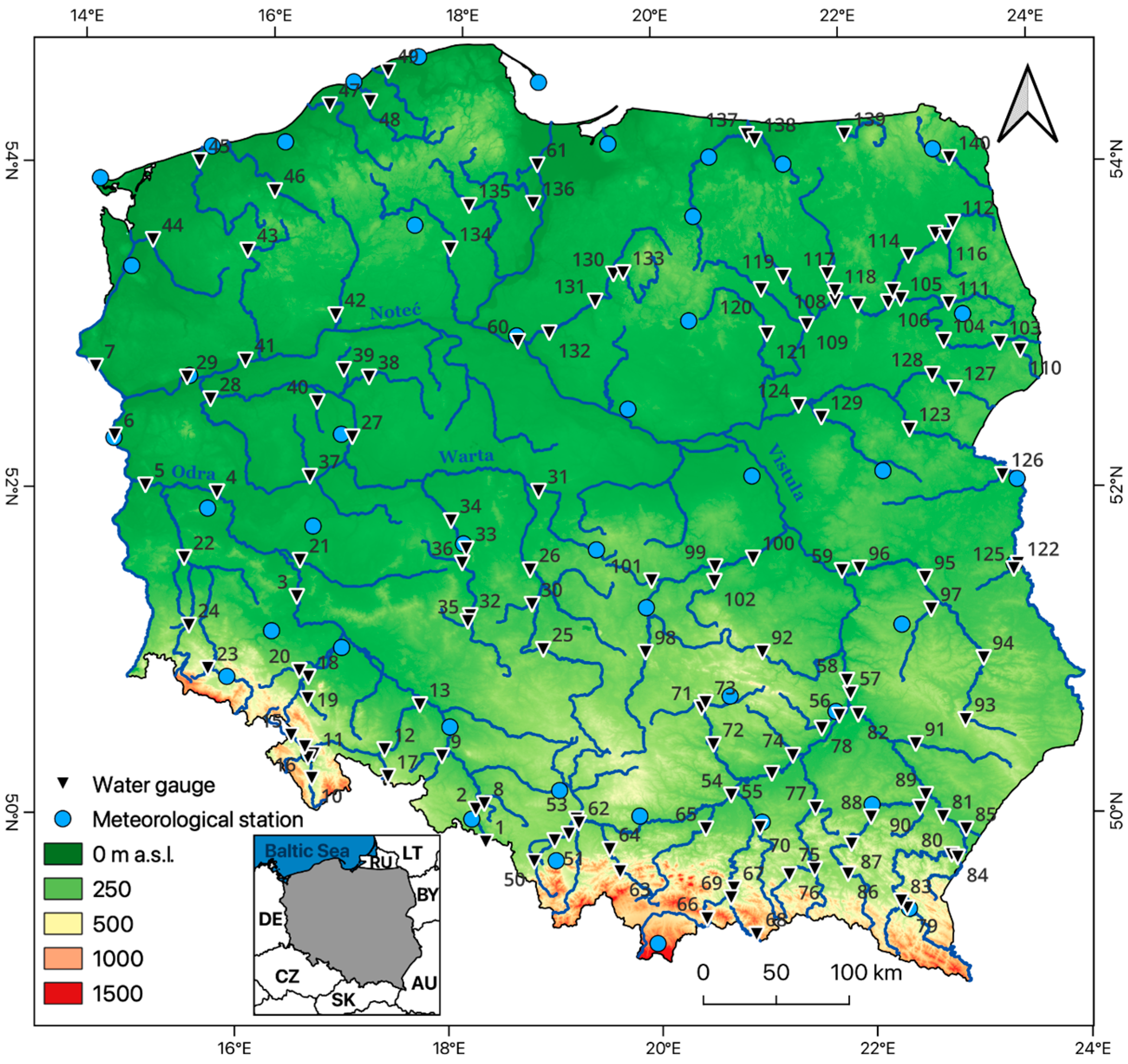
2. Materials and Methods

The paper analyzes changes in meteorological (air temperature, precipitation, and surface evaporation) and hydrological elements (runoff and ND_LF) in the multi-annual period 1951–2020 and in two sub-periods, i.e., 1951–1988 and 1988–2020, which are before and after the change in climatic conditions in Poland. The year of division (1988) was selected based on previous studies that showed clear differences in the course of selected meteorological elements before and after that year [26]. The meteorological and hydrological data used in the study were obtained from the publicly available archives of the Institute of Meteorology and Water Management—National Research Institute (IMGW-PIB) in Warsaw, Poland (https://danepubliczne.imgw.pl, accessed on 10 October 2024). Analyzes of river runoff and ND_LF were performed based on daily discharges from the multi-annual period 1951–2020, recorded in 140 water gauges located on 96 rivers in Poland (Figure 1;

Table A1. Basic hydrological characteristics of the analyzed rivers. Numbering was performed in accordance with Figure 1.

No.	River	Gauge	Catchment Area [km2]	Runoff Depth [mm]	NDLF	Trend NDLF R *	River Regime **
1	Odra	Chałupki	4666	282.4	48.8	−0.218	4
2	Odra	Racibórz-Miedonia	6744	300.8	47.6	−0.154	4
3	Odra	Ścinawa	29,584	188.9	52.1	0.168	4
4	Odra	Cigacice	40,106	170.6	56.6	0.182	2
5	Odra	Połęcko	47,370	167.1	57.8	0.175	2
6	Odra	Słubice	53,600	174.2	59.8	0.187	2
7	Odra	Gozdowice	109,729	146.9	66.2	0.161	2
8	Sumina	Nędza	94.4	191.3	56.5	0.280 *	4
9	Biała	Dobra	353	99.4	59.7	0.016	4
10	Nysa Kłodzka	Bystrzyca Kłodzka	260	466.7	45.6	0.224	4
11	Nysa Kłodzka	Kłodzko	1084	364.9	51.0	−0.150	4
12	Nysa Kłodzka	Nysa	3276	278.6	43.6	−0.115	4
13	Nysa Kłodzka	Skorogoszcz	4514	249.8	52.0	0.130	4
14	Bystrzyca Dusznicka	Szalejów Dolny	175	378.1	54.7	0.002	2
15	Ścinawka	Tłumaczów	256	279.8	57.8	−0.023	2
16	Ścinawka	Gorzuchów	511	274.8	50.5	0.191	4
17	Biała Głuchołaska	Głuchołazy	283	542.0	57.3	−0.108	4
18	Bystrzyca	Krasków	683	205.9	46.9	0.213	4
19	Piława	Mościsko	291	172.6	57.1	0.253 *	4
20	Strzegomka	Łażany	356	198.0	58.0	−0.324 *	4
21	Barycz	Osetno	4579	101.6	48.9	0.336 *	3
22	Bóbr	Żagań	4254	275.8	54.5	0.255 *	4
23	Kamienica	Barcinek	97.2	389.7	55.0	0.065	2
24	Kwisa	Nowogrodziec	736	306.9	52.7	0.261 *	4
25	Warta	Działoszyn	4088	185.8	64.6	0.293 *	2
26	Warta	Sieradz	8140	171.3	65.2	0.037	2
27	Warta	Poznań	25,126	124.5	68.3	−0.140	2
28	Warta	Skwierzyna	31,268	123.4	70.7	−0.066	2
29	Warta	Gorzów Wielkopolski	52,186	124.4	59.9	0.119	2
30	Oleśnica	Niechmirów	592	126.7	60.9	0.321 *	3
31	Ner	Dąbie	1712	181.6	44.5	−0.012	2
32	Prosna	Mirków	1255	126.0	46.4	0.296 *	2
33	Prosna	Piwonice	2938	119.2	55.4	0.091	2
34	Prosna	Bogusław	4304	114.3	48.2	0.142	2
35	Niesób	Kuźnica Skakawska	246	123.8	62.8	−0.238 *	3
36	Ołobok	Ołobok	447	110.7	60.0	0.093	3
37	Mogilnica	Konojad	663	77.3	52.8	0.109	3
38	Wełna	Pruśce	1130	92.5	65.2	0.187	3
39	Flinta	Ryczywół	276	74.1	53.4	0.222	3
40	Sama	Szamotuły	395	83.4	58.0	0.277 *	3
41	Noteć	Nowe Drezdenko	15,970	143.2	53.7	0.219	2
42	Gwda	Piła	4704	180.0	49.4	0.181	1
43	Drawa	Drawsko Pomorskie	609	209.2	76.5	−0.132	2
44	Ina	Goleniów	2163	185.5	66.6	0.174	2
45	Rega	Trzebiatów	2628	239.4	42.4	0.215	2
46	Parsęta	Tychówko	896	289.1	48.0	0.245 *	2
47	Wieprza	Stary Kraków	1519	327.0	53.5	−0.283 *	1
48	Słupia	Słupsk	1450	338.5	35.1	−0.002	1
49	Łupawa	Smołdzino	805	325.7	44.8	−0.333 *	1
50	Wisła	Skoczów	297	641.0	39.3	−0.049	4
51	Wisła	Goczałkowice	738	381.0	44.7	−0.066	5
52	Wisła	Jawiszowice	971	426.1	44.0	0.113	5
53	Wisła	Bieruń Nowy	1748	381.8	49.9	−0.351 *	4
54	Wisła	Jagodniki	12,058	334.4	51.4	0.135	4
55	Wisła	Szczucin	23,901	307.4	44.6	−0.185	4
56	Wisła	Sandomierz	31,846	284.8	49.8	−0.184	4
57	Wisła	Zawichost	50,732	261.9	45.4	−0.200	4
58	Wisła	Annopol	51,518	261.8	44.3	−0.151	4
59	Wisła	Dęblin	68,234	227.9	46.4	−0.179	4
60	Wisła	Toruń	181,033	167.5	44.4	−0.050	2
61	Wisła	Tczew	194,376	167.3	45.4	−0.124	2
62	Soła	Oświęcim	1386	473.1	45.0	0.135	4
63	Skawa	Sucha Beskidzka	468	507.9	43.6	−0.095	4
64	Skawa	Wadowice	836	465.0	47.9	0.061	4
65	Raba	Proszówki	1470	356.6	54.3	−0.247 *	4
66	Dunajec	Krościenko	1580	634.9	45.2	−0.360 *	5
67	Dunajec	Nowy Sącz	4341	472.8	44.9	−0.466 *	4
68	Poprad	Muszyna	1514	365.9	45.4	−0.220	4
69	Poprad	Stary Sącz	2071	380.5	45.6	−0.130	4
70	Biała	Koszyce Wielkie	957	290.5	47.8	−0.254 *	4
71	Nida	Brzegi	2259	177.1	56.7	0.137	2
72	Nida	Pińczów	3352	168.2	53.9	0.218	2
73	Czarna Nida	Tokarnia	1216	171.4	50.2	0.091	2
74	Czarna	Połaniec	1354	149.2	44.8	0.175	3
75	Wisłoka	Żółków	581	384.7	42.7	0.131	4
76	Ropa	Klęczany	483	406.9	67.1	−0.569 *	4
77	Brzeźnica	Brzeźnica	484	212.5	53.8	−0.066	4
78	Koprzywianka	Koprzywnica	502	127.1	45.9	−0.010	3
79	San	Lesko	1614	555.0	55.4	−0.586 *	4
80	San	Przemyśl	3686	444.9	39.0	−0.484 *	4
81	San	Jarosław	7041	312.7	48.8	−0.328 *	4
82	San	Radomyśl	16,824	241.6	54.0	−0.440 *	4
83	Osława	Zagórz	505	509.0	38.2	−0.113	4
84	Wiar	Krówniki	789	252.7	49.0	−0.162	4
85	Wisznia	Nienowice	1185	178.6	47.7	0.016	4
86	Wisłok	Krosno	596	327.8	47.9	−0.475 *	4
87	Wisłok	Żarnowa	1427	287.3	49.0	−0.384	4
88	Wisłok	Rzeszów	2086	263.1	43.4	−0.064	4
89	Wisłok	Tryńcza	3516	227.7	51.1	−0.228	4
90	Mleczka	Gorliczyna	529	173.2	45.3	−0.076	4
91	Tanew	Harasiuki	2034	189.7	53.9	−0.030	2
92	Kamienna	Wąchock	476	192.7	44.0	0.252 *	2
93	Wieprz	Zwierzyniec	405	160.1	66.3	−0.238 *	1
94	Wieprz	Krasnystaw	3001	129.8	59.0	−0.440 *	2
95	Wieprz	Lubartów	6364	111.7	58.8	−0.196	2
96	Wieprz	Kośmin	10,231	113.2	54.5	−0.295 *	2
97	Bystrzyca	Sobianowice	1265	125.6	59.2	−0.334 *	2
98	Pilica	Przedbórz	2536	185.9	56.6	0.430 *	2
99	Pilica	Nowe Miasto	6717	166.9	50.8	0.415 *	2
100	Pilica	Białobrzegi	8664	160.4	49.9	0.139	2
101	Wolbórka	Zawada	616	137.5	44.0	−0.064	2
102	Drzewiczka	Odrzywół	1004	166.9	44.0	0.285 *	2
103	Narew	Narew	1978	146.0	56.9	−0.521 *	3
104	Narew	Suraż	3376	139.5	62.2	−0.387 *	3
105	Narew	Strękowa Góra	7181	141.4	59.8	−0.332 *	3
106	Narew	Wizna	14,308	148.4	63.6	−0.248 *	3
107	Narew	Piątnica-Łomża	15,296	150.9	65.4	−0.240 *	3
108	Narew	Nowogród	20,106	152.4	58.0	−0.275 *	3
109	Narew	Ostrołęka	21,862	155.8	55.5	−0.206	3
110	Narewka	Narewka	590	156.9	56.3	0.167	3
111	Supraśl	Fasty	1817	153.3	48.6	−0.258 *	2
112	Biebrza	Sztabin	846	171.5	62.1	0.005	3
113	Biebrza	Dębowo	2322	167.3	56.7	−0.226	3
114	Biebrza	Osowiec	4365	160.0	62.2	−0.051	3
115	Biebrza	Burzyn	6900	158.0	61.1	−0.192	3
116	Brzozówka	Karpowicze	650	154.1	52.0	−0.062	3
117	Pisa	Ptaki	3562	181.6	68.5	−0.058	1
118	Pisa	Dobrylas	4061	182.4	68.2	−0.016	2
119	Rozoga	Myszyniec	231	155.2	49.0	−0.024	2
120	Omulew	Krukowo	1265	170.0	49.9	0.243 *	2
121	Orzyc	Krasnosielc	1268	142.2	49.1	−0.056	2
122	Bug	Włodawa	14,410	120.5	72.8	−0.375 *	3
123	Bug	Frankopol	31,336	118.1	68.8	−0.394 *	3
124	Bug	Wyszków	39,119	122.5	65.3	−0.347 *	3
125	Włodawka	Okuninka	576	116.5	61.3	−0.204	3
126	Krzna	Malowa Góra	3128	108.1	52.0	−0.420 *	3
127	Nurzec	Boćki	556	134.0	44.8	−0.092	3
128	Nurzec	Brańsk	1227	126.8	45.2	0.192	3
129	Liwiec	Łochów	2466	134.1	43.0	−0.149	3
130	Drwęca	Nowe Miasto Lubawskie	2725	188.9	68.9	−0.144	2
131	Drwęca	Brodnica	3526	192.5	63.9	0.093	2
132	Drwęca	Elgiszewo	4959	173.7	69.4	0.155	2
133	Wel	Kuligi	764	206.3	56.7	0.127	1
134	Brda	Tuchola	2462	248.6	40.5	0.143	1
135	Wda	Czarna Woda	940	210.7	57.4	−0.261 *	1
136	Wierzyca	Brody Pomorskie	1544	175.0	49.4	0.024	2
137	Łyna	Sępopol	3647	211.7	43.7	0.133	2
138	Guber	Prosna	1568	171.6	48.8	−0.041	2
139	Gołdapa	Banie Mazurskie	548	266.9	54.1	−0.074	3
140	Czarna Hańcza	Czerwony Folwark	454	262.6	64.6	−0.033	2

Note: * R statistically significant at p < 0.05; ** types of river flow regimes: 1—nival poorly developed; 2—nival moderately developed; 3—nival strongly developed; 4—nival-pluvial; 5—pluvial-nival. Source: adapted from [48].

).

Surface evaporation (Ev, mm of water column equivalent) in a given month from the area of Poland was calculated with the help of the Ivanov formula (after [35]):

Ev = 0.0018 × (25 + t)² × (100 − f),

(1)

where t is the average monthly temperature (°C) and f is the monthly relative humidity (%), in which arguments of function (1) are the area means of annual air temperature (T_PL) and relative humidity (f_PL) in Poland.

The method of estimating surface evaporation using the formula proposed by Ivanov performs satisfactorily in Poland (e.g., [36,37,38,39]). Annual surface evaporation was calculated as the sum of monthly evaporation. Using a series of annual Ev values, the approximate water balance in a given calendar year was estimated as the difference between annual precipitation (P_PL) and annual evaporation (Ev) in Poland, without taking into account retention.

Daily discharge was used to calculate the number of days with flows below the 10th percentile (Q₁₀) in the hydrological year (in Poland lasting from 1 November to 31 October) in three temporal variants: the entire multi-annual period 1951–2020 and two sub-periods, i.e., before (1951–1988) and after climate change (1988–2020). Then, the trends of their changes and statistical significance were examined.

In order to examine the occurrence of low flows in rivers in Poland, the threshold level method was applied. This is one of the most common methods used in low flows research [40,41]. In our study, we used the 10th percentile (Q₁₀) from the sum flow curve with the lower values, which corresponds to the 90th percentile (Q₉₀) from the sum flow curve with the higher values. The low-flow periods were characterized with the use of the number of days with low flows (ND_LF) below a threshold value, which was adopted as the 0.1 (10%) percentile (Q₁₀) from the set of daily flows in 1951–2020. In our study, low flow was defined as the period during which the flows were equal to or lower than the adopted threshold value. Based on the daily flow dataset from 1951 to 2020, we assumed the threshold value to be the 0.1 (10%) percentile (Q₁₀) of the sum flow curve with the lower values, which corresponds to the 90th percentile (Q₉₀) from the sum flow curve with the higher value.

In the next stage, the change trends in the number of days with flows below Q₁₀ detected in the respective gauges and their statistical significances were determined. The differences in the duration of low flows below Q₁₀ between the period after climate change (1988–2020) and the period before it (1951–1988) were also determined.

The average ND_LF was calculated based on the sum of the number of low flow days over the entire multi-annual period, which was then divided by the number of years, in which they occurred.

In the next stage, the linear regression method was used to determine the long-term trends in the ND_LF and their statistical significance at three levels: 0.05, 0.01, and 0.001. The critical values of the correlation coefficient for these significance levels for the entire multi-annual period 1951–2020 and the two sub-periods were derived from the statistical tables (

Table 1. Limit values of correlation coefficients for various levels of statistical significance for the periods studied.

Significance Level (p)	1951–2020 (70 Years)	1951–1988 (38 Years)	1988–2020 (33 Years)
0.05	0.232	0.213	0.334
0.01	0.302	0.403	0.430
0.001	0.380	0.501	0.532

).

In order to determine changes in the investigated hydro-meteorological elements during the warming period (1988–2020) relative to the period 1951–1988, the change index was computed (Equation (2)):

$$S_{{\overline{X}}_{1988-2020}-{\overline{X}}_{1951-1988}}={\displaystyle \frac{{\overline{X}}_{1988-2020}-{\overline{X}}_{1951-1988}}{{\overline{X}}_{1951-1988}}}\cdot 100\%$$

(2)

where $S_{{\overline{X}}_{1988-2020}}$ and $S_{{\overline{X}}_{1951-1988}}$ are the average values of hydro-meteorological elements in the separated sub-periods of the multi-annual period 1951–2020.

The calculated index shows the percentage increase or decrease of the analyzed elements in the period after climate change (1988–2020) in relation to their values in the period preceding it (1951–1988). The differences in the annual values of hydro-meteorological elements between 1988–2020 and 1951–1988 were calculated. The statistical significance of these differences was tested using the t-test for independent samples. Each time, the hypothesis H₀:μ1 = μ2 of equality of expected values was tested against H₁:μ1 ≠ μ2. Rejection of the hypothesis allowed us to conclude on significant differences in the average maximum river runoff observed after and before climate change. The t-statistic has a Student’s t-distribution, with n₁ + n₂-2 degrees of freedom (Equation (3)):

$$T={\displaystyle \frac{{\overline{X}}_1-{\overline{X}}_2}{S_{{\overline{X}}_1-{\overline{X}}_2}}} ,$$

(3)

where $S_{{\overline{X}}_1-{\overline{X}}_2}$ is written as follows (Equation (4)):

$$S_{{\overline{X}}_1-{\overline{X}}_2}=\sqrt{{\displaystyle \frac{{{\left(n_1-1\right)·S}_1^2+\left(n_2-1\right)·S}_2^2}{n_1+n_2-2}}·\left({\displaystyle \frac{1}{n_1}}+{\displaystyle \frac{1}{n_2}}\right)},$$

(4)

where $n_1$ and $n_{2 }$ are sample sizes, $S_1^2$ and $S_2^2$ are variances of both samples, and $\overline{X_1}$ and $\overline{X_2}$ are mean values of both samples.

In further analysis, in order to detect spatial regularities of long-term changes in the ND_LF, the cluster analysis method [42] was used to group the gauges according to the values of 70 annual ND_LF. The grouping results were presented in the form of a dendrogram, which reflected the similarity structure of the studied set of gauges and was used to separate typological classes. In the study, the number of classes was determined based on the analysis of the dendrogram geometry and the linkage distance curve. In the procedure of verifying the optimal number of clusters, the GWZ distance criterion [43] and the “Mojena rule” [44] were used. These methods usually give satisfactory results of unambiguous division into the number of classes [45] and are recommended for use in cluster analyses by many experts (e.g., [46]).

The application of hierarchical cluster analysis, which is a key element in minimizing differences within clusters, resulted in distinguishing two groups of gauges, designated as A and B, respectively. Group B was additionally split into two sub-groups: B1 and B2. The mathematical and statistical calculations were performed with the help of Statistica 13 software licensed by Statsoft^®.

3. Results

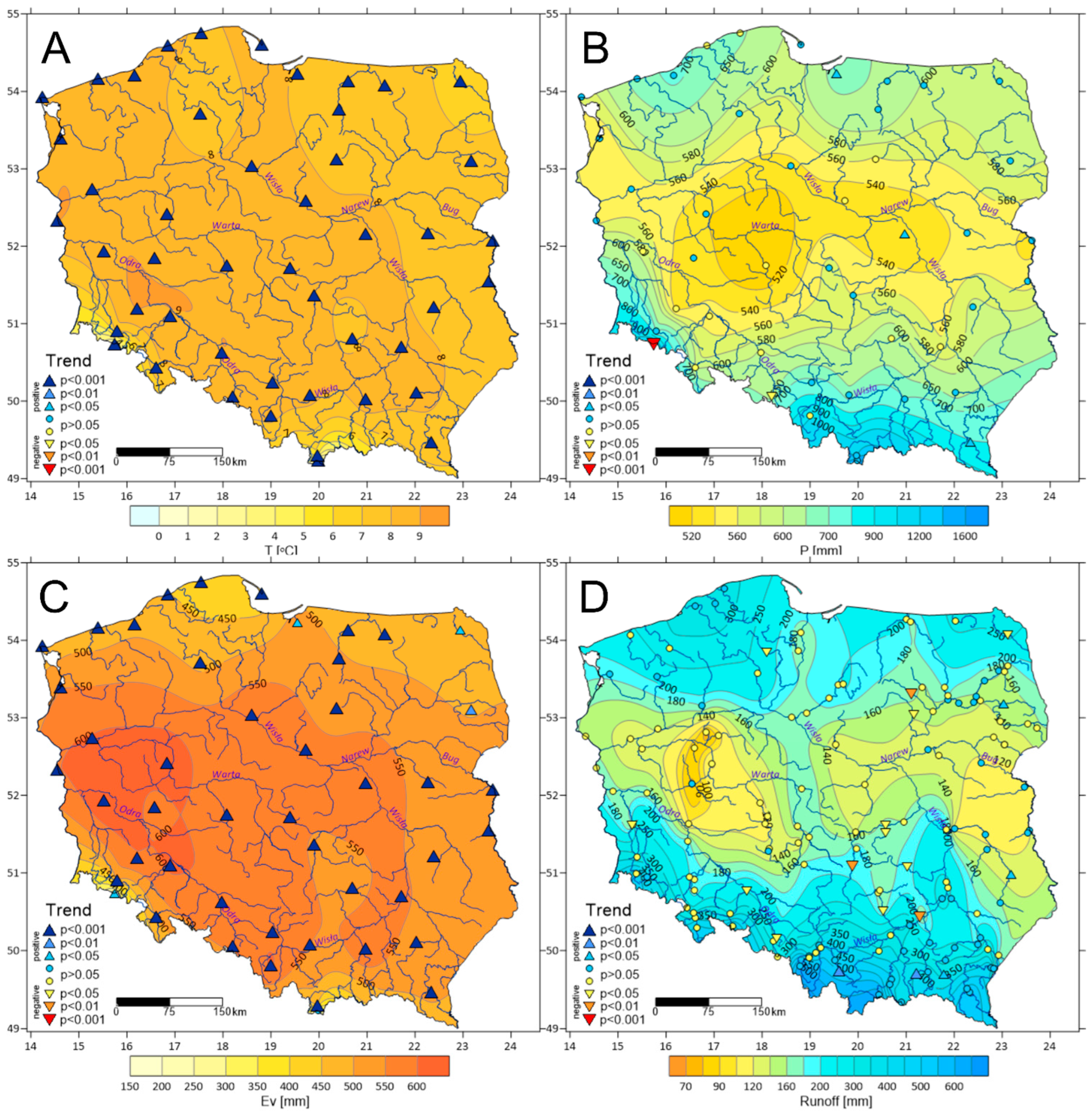
3.1. Changes in the Average Values of Hydro-Meteorological Elements in Poland in 1951–2020

The highest average air temperatures, exceeding 9 °C, were recorded in South-western Poland, with temperatures decreasing towards the east and in mountainous areas (Figure 2). Evaporation also showed a similar spatial distribution (Figure 2). The central part of Poland was characterized by relatively lowest annual precipitation totals, which increased towards the north and south; a similar relationship can be seen in the case of river runoff (Figure 2). Both the average annual air temperatures and evaporation showed strong increasing trends throughout the country, in most cases statistically significant at the level of p < 0.001 (Figure 2). The situation is different in the case of precipitation totals and river runoff—in most of the analyzed locations, the trends were statistically insignificant (p > 0.05); however, increasing trends of runoff (p < 0.01) were concluded in South-western Poland (Figure 2).

A comparison of the average values of the hydro-meteorological variables studied between the sub-periods of the analyzed multi-annual period, i.e., 1951–1988 and 1988–2020, was also performed, and the statistical significance of the obtained differences was examined (Figure 3). The average air temperatures increased after 1988 throughout Poland from 0.9 to over 1.3 °C (Figure 3A). Similar changes were determined for evaporation, which increased by about 10–25% (Figure 3C). For both air temperature and evaporation, the statistical significance of the changes was very high, mostly at the level of p < 0.001 (Figure 3A,C). Precipitation did not show such changes—a statistically significant decrease in precipitation totals (by over 5%) was recorded only in the southern part of the Odra River basin, and in most stations, statistically insignificant increases in values were recorded (Figure 3B). The most complex changes spatially occurred in the case of river runoff—most of Poland was characterized by a decrease in runoff after 1988 by about 5–15%, of which some changes were statistically significant (Figure 3D). In the south-eastern part of the country, primarily in the catchments of the right tributaries of the Vistula River, an increase in runoff by about 5–10% was recorded, but only in the case of one gauge, these changes were statistically significant (Figure 3D).

Taking into account the entire studied multi-annual period, statistically significant decreasing trends of ND_LF in the eastern and southern parts of the Vistula River basin were clearly visible—such trends were characteristic of the whole Poland in the first sub-period (1951–1988) (Figure 4). After 1988, the situation changed, and an increase in ND_LF (statistically significant in selected rivers) was observed in most stations (Figure 4). The exceptions are several rivers in Southern Poland, for which statistically significant decreasing trends of ND_LF were noted.

Annual ND_LF was correlated with average annual air temperature (Figure 5A), evaporation (Figure 5B), and precipitation totals (Figure 5C). In the case of air temperature, both positive (for most of the study area) and negative correlations (mainly for the right part of the Vistula River basin) can be determined (Figure 5A). Correlations of annual ND_LF with evaporation were only positive and statistically significant over most of Poland; the exception is again the southern and eastern parts of the Vistula River basin, where the strength of correlation was lower and more trends did not show statistical significance (Figure 5B). The correlation of annual ND_LF with precipitation totals was negative over the entire country and in many cases statistically significant at the level of p < 0.001 (Figure 5C).

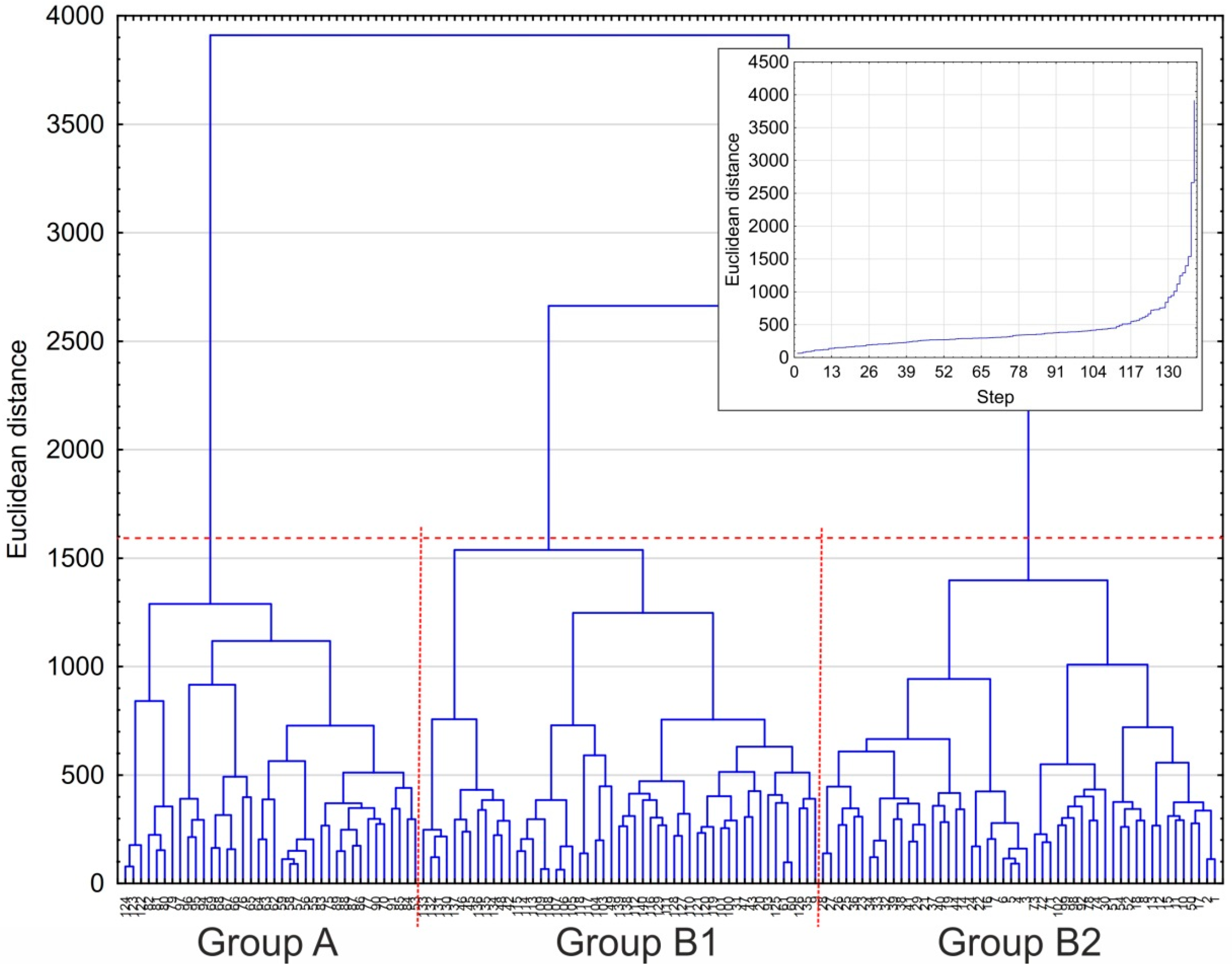
3.2. Results of the Procedure for Grouping Water Gauges Based on the Number of Days with Low Flows

One hundred and forty series of the ND_LF in a year were subjected to the agglomeration procedure performed with the use of Ward’s method. The Euclidean distance was used as a measure of taxonomic distance. The distance was calculated with the use of Equation (5):

$$\mathrm{ESS}={\sum }_{j=1}^K(x_j-\overline{x})’(x_j-\overline{x}),$$

(5)

where K is the number of clusters, $x_j$ is the multivariate measurement associated with the jth item, and $\overline{x}$ is the mean of all items.

This type of procedure revealed the typological diversity of the analyzed set. The graphical results of this grouping are presented in Figure 6.

The number of individual taxonomic levels of grouping was different in individual clusters. The analysis showed that in the case of lower levels of grouping, the aggregation into a cluster was the result of the location of series of gauges at small distances from each other—either on the same stream or in catchments located close to each other. In some cases, in a given cluster at the 3rd, 4th, or 5th grouping level, there were single gauges located in distant areas, whose variance of the ND_LF was similar to the variance in catchments located close to each other.

The highest taxonomic level of grouping revealed that there were two groups of gauges on Polish rivers differing in terms of the variance of the ND_LF. The number of gauges in each of these groups was noticeably diversified: group A consisted of only about 25% of all analyzed gauges, while group B consisted of 75% of all analyzed gauges. It can be noticed that at a lower taxonomic level, group B was divided into two sub-groups that differed from each other, designated as B1 and B2, respectively (Figure 6).

The analysis of the differentiation at the highest taxonomic levels (ESS = 1600) revealed a large differentiation of the variance of the ND_LF in gauges in Poland. This issue seemed important, so our further analysis will be devoted to it. The similarity of the characteristics of flow distributions in closely located gauges, either on the same stream or in two small catchments located close each other, was obvious and did not require further studies. For this reason, the differentiation of the ND_LF at lower levels of grouping will not be addressed here.

The statistical characteristics of the ND_LF in individual groups are presented in

Table 2. The average numbers of days with low flows per year (ND_LF) in individual groups and statistical characteristics of their differentiation (1951–2020).

Group	Mean	BSS	Standard Deviation (σ)	Median	Min.	Max.	Lower Quartile	Upper Quartile
A (SE Poland)	36.07	3.47	29.05	30.61	0.42	127.97	13.42	49.70
B1 (N Poland)	35.98	4.19	35.05	21.83	0.15	136.28	10.70	52.38
B2 (SW Poland)	35.56	3.97	37.25	25.36	1.21	124.63	8.96	58.60

Note: mean—the average annual ND_LF in a given group; BBS—standard error of a given mean (days); min. and max.—the minimum and maximum ND_LF in a given group, respectively; lower quartile and upper quartile—values corresponding to 25 and 75% of the series of the ND_LF, respectively; median—middle value of the set.

.

The average numbers of days with low flows per year in the multi-annual period 1951–2020 were very similar in all these groups (Table 2), and the differences between them were statistically insignificant. However, the analysis of the distributions of values in individual groups revealed that there were some differences between them, and these constituted an internal differentiation of the set, revealed in the agglomeration procedure. The values of the correlation coefficients between the series of average numbers of days with low flows between groups were highly significant, but of moderate strength (group A and sub-group B1: r = 0.56, p << 0.001; group A and sub-group B2, r = 0.47, p << 0.001). The correlation between sub-groups B1 and B2 was clearly stronger and also highly significant (r = 0.73, p << 0.001).

The distribution of correlation coefficients between the series of ND_LF in a year explained that the basic framework for shaping the ND_LF in a year in Poland was formed under the influence of common factors, which, however, showed quite clear variability in individual areas (Figure 7).

Such very similar statistical characteristics of the individual groups suggest that internal differences of the set are the reason for the separation of respective types, resulting either from regional differentiation or from differentiation of the ND_LF courses in individual sub-sets.

3.3. Regional Differentiation in the Number of Days with Low Flows in Poland

In order to explain this issue and obtain a picture of the spatial differentiation of ND_LF, individual gauges were plotted on the map (Figure 8), in accordance with their geographical coordinates and association with a specific group.

The ND_LF in individual gauges classified into respective types (groups) formed relatively homogenous territorial groups spatially. This means that the detected individual types of the ND_LF showed clear regional differentiation. In the border areas between two different groups, there were few cases of “overlapping” of gauges belonging to different groups (e.g., along the Bug River). Such a situation in border zones is typical, as physical-geographical boundaries are zones, not lines. There are few examples of gauges classified in the grouping procedure to a specific group, but located in area typical to another group, e.g., while located in the area belonging to group A, the Zwierzyniec gauge at the Tanew River was classified into sub-group B1, and located in the area belonging to sub-group B2, the Dobra gauge at the Biała River was designated to sub-group B1.

The distinguished group A covered relatively the smallest part of Poland. It included the south-eastern part of the country, and its borders were marked from the south and east by the state border, to the west by the Soła River and the Vistula River, and to the north by the course of the Bug River—from the state border to the Wyszków gauge. This area will be referred to as “South-Eastern (SE) Poland” hereinafter.

Group B covered the remaining part of the country, with sub-group B1 covering the Northern and North-eastern Poland that included the regions of Pomerania and Warmia, the lower Vistula River, and the Masurian Lake District. The southern border of the area covered by sub-group B1 ran from Western Pomerania through the area between the Warta and middle Vistula rivers to the Bug River and the state border. Sub-group B2 covered the area from the western borders of Poland to the Silesian Beskids, following the Soła River and then along the Vistula River to the area where the Pilica River flowed into the Vistula. The area covered by gauges belonging to sub-group B1 will be referred to as “Northern (N) Poland”, and the area covered by sub-group B2 will be referred to as “South-Western (SW) Poland”.

3.4. Formal Reasons for Spatial Differentiation of the Number of Days with Low Flows in Poland

A more detailed analysis of the patterns of average ND_LF allowed us to indicate the basic reasons for splitting all gauges in Poland into two groups, representing separate types of low flow patterns.

The most important reason for the formation of two separate types in the ND_LF set was differences in the nature of the variability of the course of the ND_LF. The analysis of linear trends in each of the areas, but (i.e., in each group) carried out in each area separately for the years 1951–1988 and for the years 1988–2020, i.e., in the sub-periods before and after climate change, revealed the basic difference in their course between groups A and sub-groups B1 and B2 (Figure 9, Figure 10 and Figure 11).

For the gauges included in the first group (Figure 9), a dual time distribution of linear trends was typical in each of these sub-periods: in the first sub-period (1951–1988), the trend in the ND_LF was negative and statistically significant (p = 0.012), while in the second sub-period (1988–2020), the trend was close to zero; there was a very weak and insignificant (p = 0.738) negative trend, and the hypothesis that it was different from zero could not be rejected.

Similarly, a dual trend distribution was also typical for the course of the ND_LF for gauges included in the second group (Figure 10 and Figure 11). The formal feature that caused the “separation” of the set of stations of group B from group A in the agglomeration procedure was the different behavior of trends in the years 1988–2020 between these groups.

In the set of the ND_LF of group B in the years 1988–2020, contrary to group A, there was not a very strong, but statistically significant (p = 0.047 (group A) and 0.048 (group B)) positive trend. Further differentiation of group B into sub-groups B1 and B2 in a greater extent was due to differences in the course of the ND_LF in the sub-period 1951–1988 rather than in 1988–2020. This is clearly visible in the comparison of Figure 5 and Figure 6. As a result of the changes in trends in both periods, the average ND_LF in individual areas changed (

Table 3. Average numbers of days with low flows (ND_LF) in the areas of occurrence of group A and sub-groups B1 and B2 in the years 1951–1988 (before climate change) and 1988–2020 (after climate change).

Group	1951–1988		1988–2020
	Average NDLF	BSS	Average NDLF	BSS
A (SE Poland)	42.17	5.29	28.81	3.86
B1 (N Poland)	36.42	6.10	34.40	5.66
B2 (SW Poland)	27.55	4.37	44.09	6.53

).

In group A, the average ND_LF in the sub-period 1988–2020 decreased noticeably (by 13.36 days per year) compared to the average ND_LF in the sub-period 1951–1988 (statistically significant decrease). In group B1, it did not change significantly (the difference of −2.02 days per year was statistically insignificant), and in group B2, it increased remarkably (by 16.54 days per year). Comparing the average ND_LF values in the individual sub-periods (Table 2), it can be concluded that, between the sub-periods 1951–1988 and 1988–2020, there was a “swap” of the area with the highest ND_LF from SE Poland (group A) to SW Poland (sub-group B2), with no significant response of ND_LF to the climate changes in N Poland (sub-group B1).

In general, in the years 1951–1988, the ND_LF showed a tendency to decrease irregularly throughout Poland. This tendency was stronger in Northern Poland and slightly weaker in the rest of the country. After 1988, the ND_LF stopped decreasing in SE Poland and began to increase in the rest of the country, most rapidly in its western and south-western parts and in Central Poland.

Based on these findings, it can be concluded that the most important reason differentiating Poland in terms of the variability of the ND_LF is the different response of individual catchment groups to the rapid climate change that occurred in 1987–1989 [29,47].

4. Discussion and Conclusions

The study revealed different directions of changes of low river flows in Poland in the multi-annual period 1951–2020, occurring under the influence of regionally differentiated climatic changes. Three groups of rivers were distinguished, different in terms of changes in ND_LF. These rivers constitute relatively homogenous regions located in the south-eastern, northern, and south-western parts of the country.

It can be assumed that the separation of these three groups of rivers in terms of different long-term changes in ND_LF is mainly influenced by climatic conditions. In the analyzed multi-annual period 1951–2020, rivers of group A were characterized by a significant decreasing trend in ND_LF. This referred to the whole hydrological year and also the winter and summer half-years. Contrary to group A, rivers of sub-groups B1 and B2 showed a predominantly increasing trend in ND_LF. In the years 1951–1988, ND_LF on most of the studied rivers decreased significantly, especially in the summer half-year (May−October). On the other hand, in the years 1988–2020, ND_LF of rivers of sub-groups B1 and B2 showed a clearly increasing trend. This is different in the case of rivers of group A; ND_LF values of these rivers showed both increasing, but statistically insignificant, and decreasing trends.

In the south-eastern part of Poland (group A), the smallest changes (increases) in air temperature and evaporation were observed. These were the only rivers that stood out in the period of warming after 1988 with higher runoff. This explained why the ND_LF of these rivers showed a decreasing trend. As a result of the change in annual runoff, the ND_LF also changed significantly. In the period of warming after 1988, the increase in runoff concerned only the Carpathian tributaries of the Vistula River, which belonged to group A (Figure 3D). The ND_LF correlations with air temperature were negative only in the case of rivers assigned to group A, and for the Carpathian tributaries, these correlations were statistically significant (Figure 5A). As a result, the ND_LF correlations of these rivers with evaporation also clearly differed from those in the other regions of the country (Figure 5B). The correlations were positive but were the weakest and often statistically insignificant. On the other hand, the ND_LF of most of the studied rivers was strongly negatively correlated with the precipitation totals, and the rivers of group A did not differ significantly from this regularity (Figure 5C). The distinction between sub-group B1 with a relatively smaller increase in ND_LF and sub-group B2 with a clear increase in ND_LF of more than 30 days was mainly driven by changes in pluvial conditions. In the south-western part of Poland, precipitation decreased in the period after 1988 (Figure 3B). Most of the rivers of group B2 were located there. This was also confirmed by stronger, statistically significant negative correlations of ND_LF with precipitation over the entire multi-annual period 1951–2020 (Figure 12).

The ND_LF values of rivers of groups A and B1 showed strong, but less statistically significant relationships with precipitation in the subsequent 20-year sub-periods of the multi-annual period 1951–2020. On the other hand, clearly stronger and statistically significant relationships between ND_LF values of rivers of sub-groups B1 and B2 and evaporation were observed over the entire period 1951–2020.

Generally, major findings of this research are as follows:

• In the multi-annual period 1951–2020, the average annual air temperature and evaporation showed strong increasing trends in Poland, in most cases statistically significant at the level of p < 0.001. In the case of precipitation totals and river runoff, the situation was different: in most locations, the trends were statistically insignificant (p > 0.05); however, increasing trends of runoff (p < 0.01) were concluded in south-western Poland.
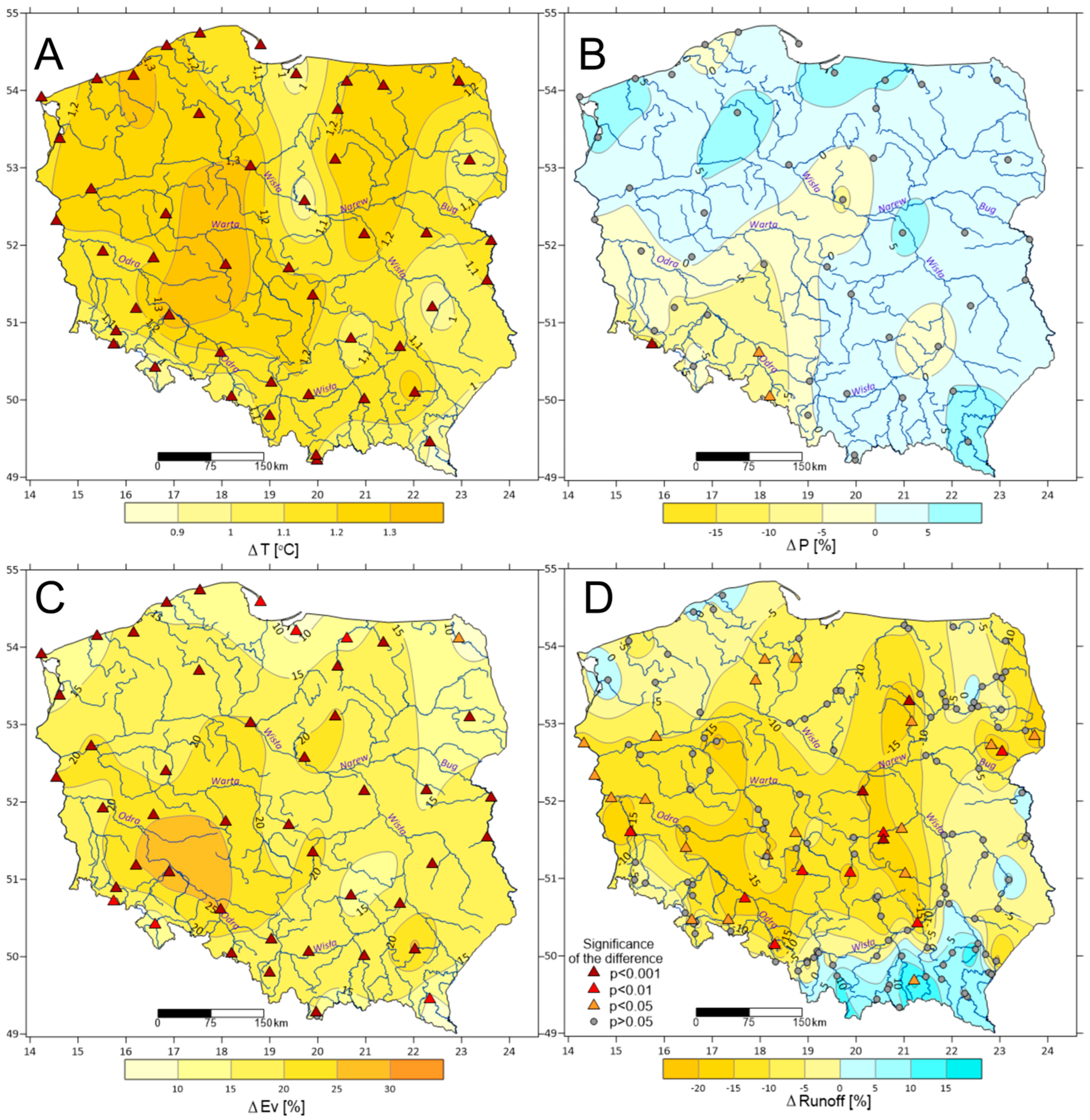
• After 1988, the average air temperature increased throughout Poland from 0.9 to over 1.3 °C. Similar changes were determined for evaporation, which increased by about 10–25%. For both air temperature and evaporation, the statistical significance of the changes was very high, mostly at p < 0.001. In turn, such changes were not detected in the case of precipitation, with a statistically significant decrease by over 5% recorded only in the southern part of the Odra River basin. In most stations, statistically insignificant increases in precipitation totals were recorded. The most complex changes spatially occurred in the case of river runoff, with most of Poland characterized by a decrease in runoff after 1988 by about 5–15%, of which some changes were statistically significant. In the south-eastern part of the country, an increase in runoff by about 5–10% was recorded, but only in the case of one gauge, these changes were statistically significant.
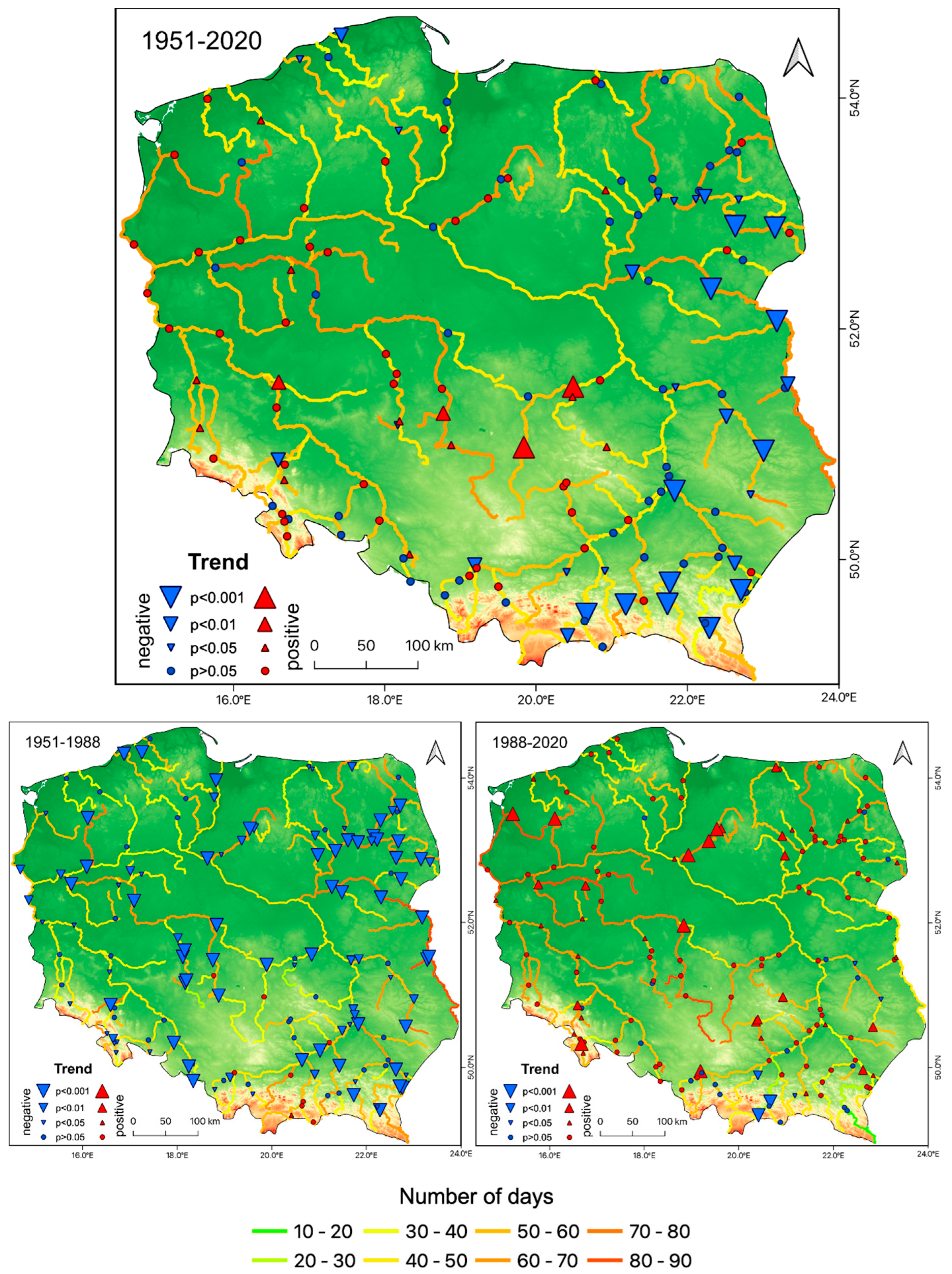
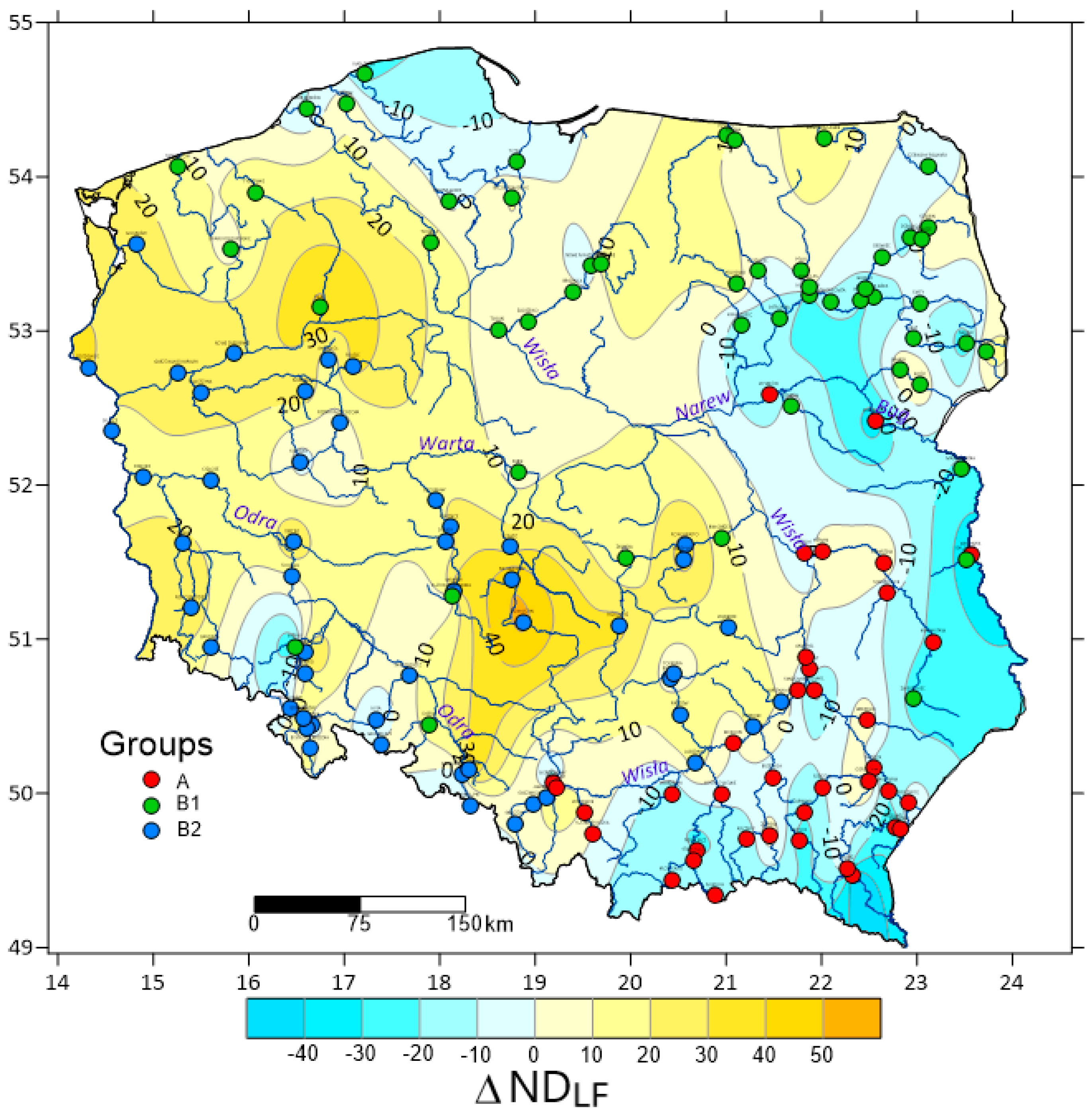
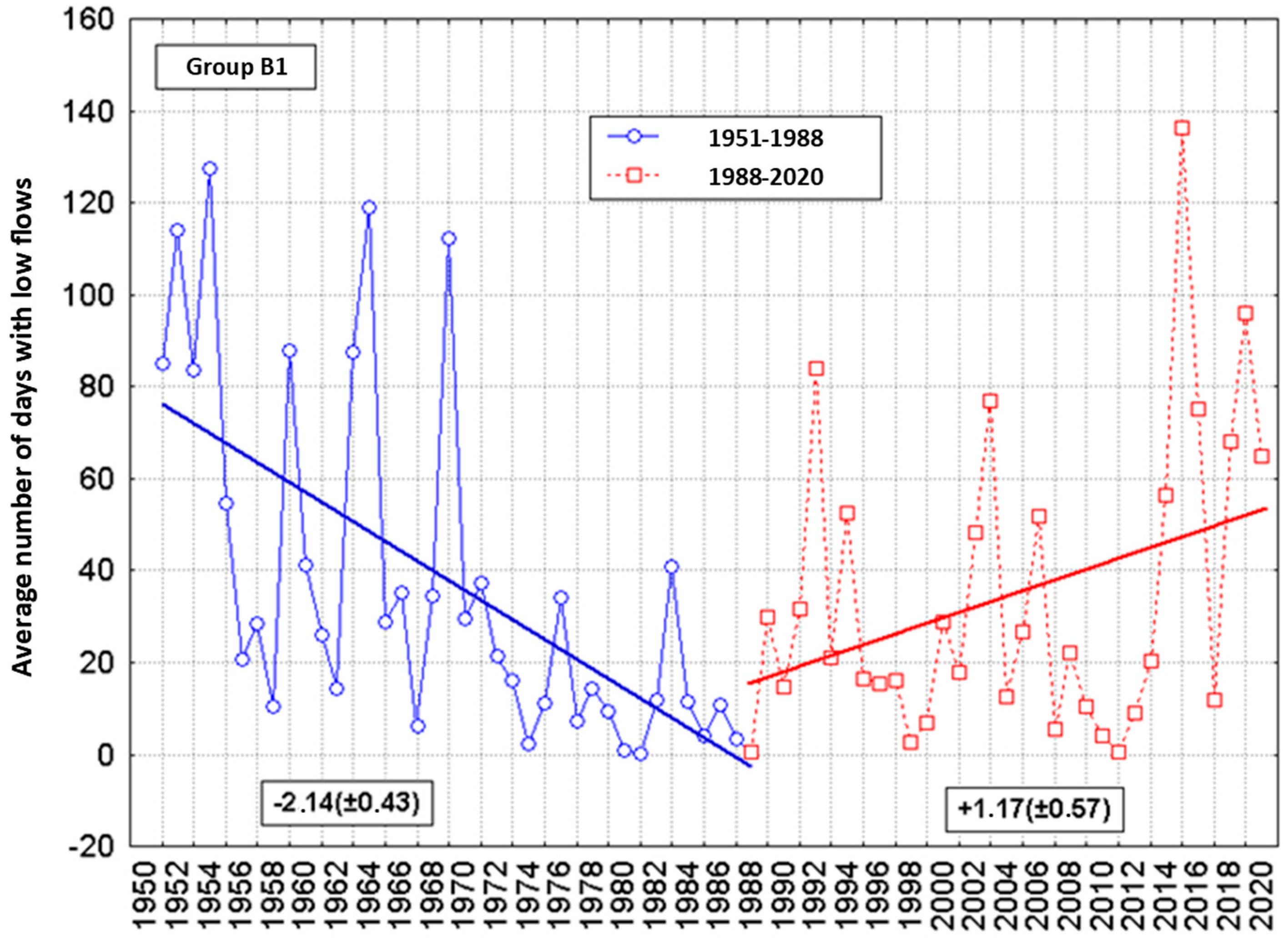
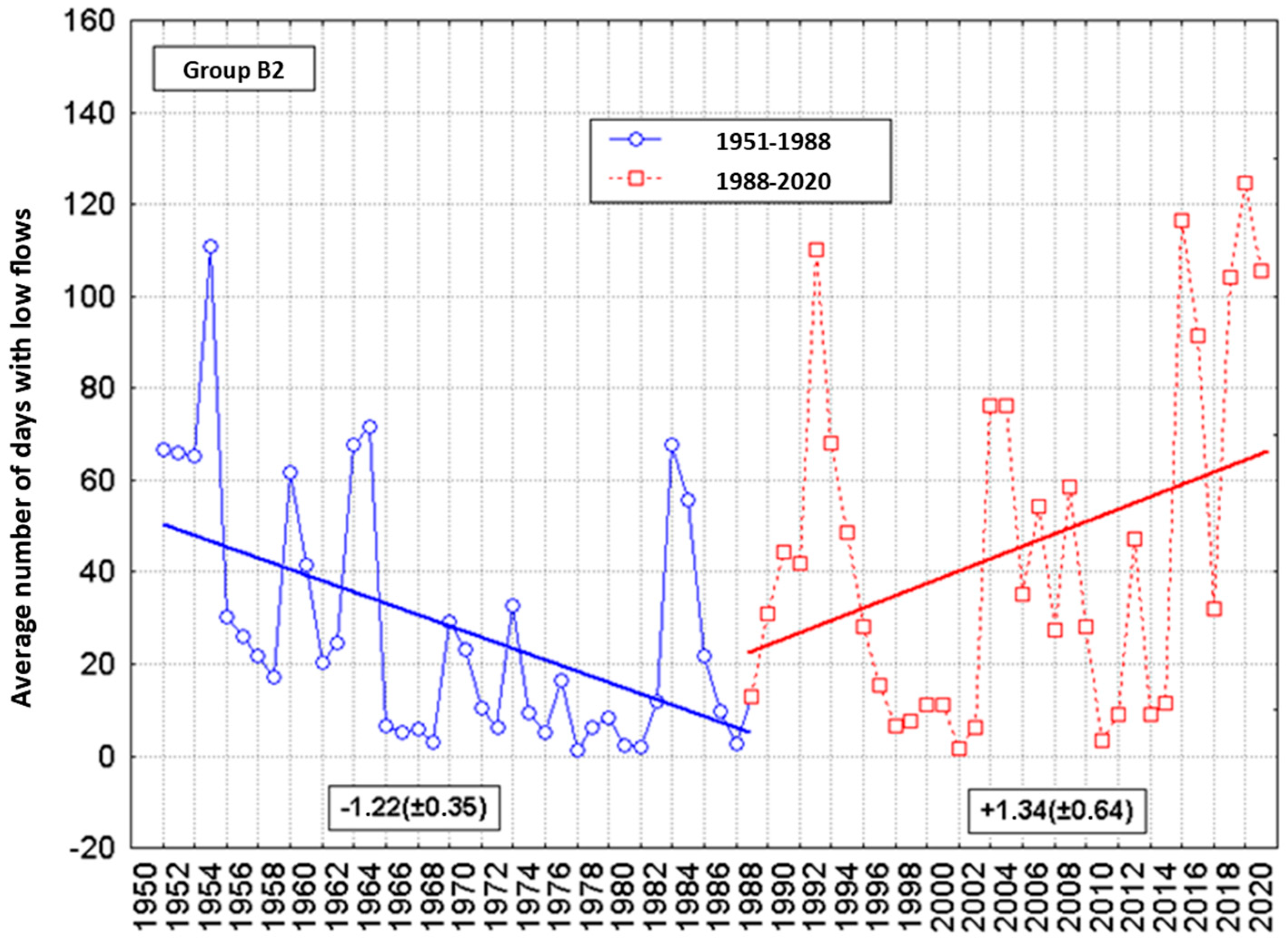
• Statistically significant decreasing trends of ND_LF in the eastern and southern parts of the Vistula River basin were concluded, and such trends were characteristic of the whole Poland in the first separated sub-period (1951–1988). After 1988, a statistically significant increase in ND_LF was observed in most stations along selected rivers, with some exceptions, including rivers in Southern Poland, where statistically significant decreasing trends of ND_LF were detected.
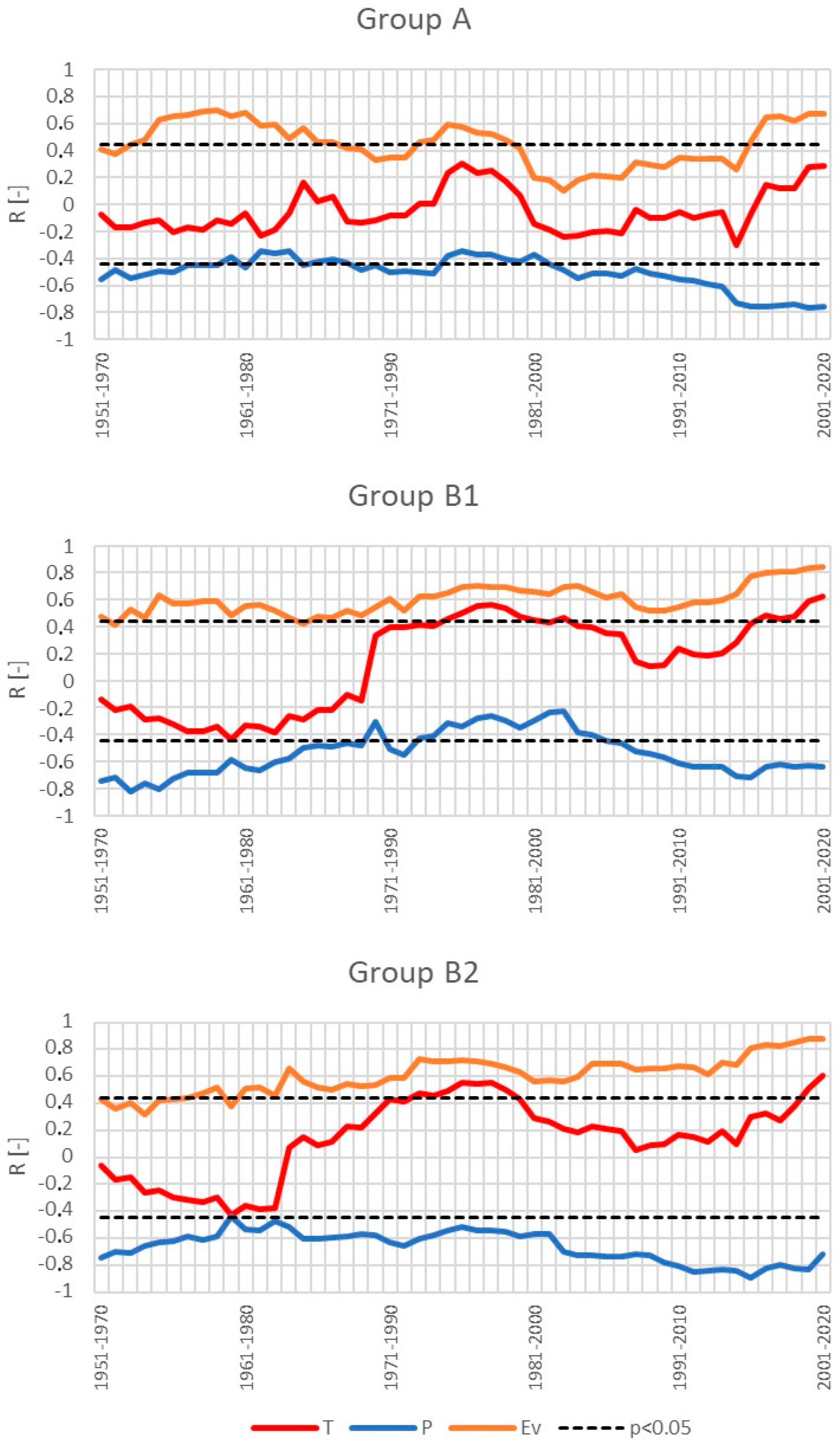
• Annual ND_LF was correlated with average annual air temperature, evaporation, and precipitation. In the case of air temperature, both positive (for most of the study area) and negative correlations (mainly for the right part of the Vistula River basin) were determined. Correlations with evaporation were positive and statistically significant over most of Poland; the southern and eastern parts of the Vistula River basin was an exception. The correlation of annual ND_LF with precipitation totals was negative over the entire Poland and in many cases statistically significant (p < 0.001).
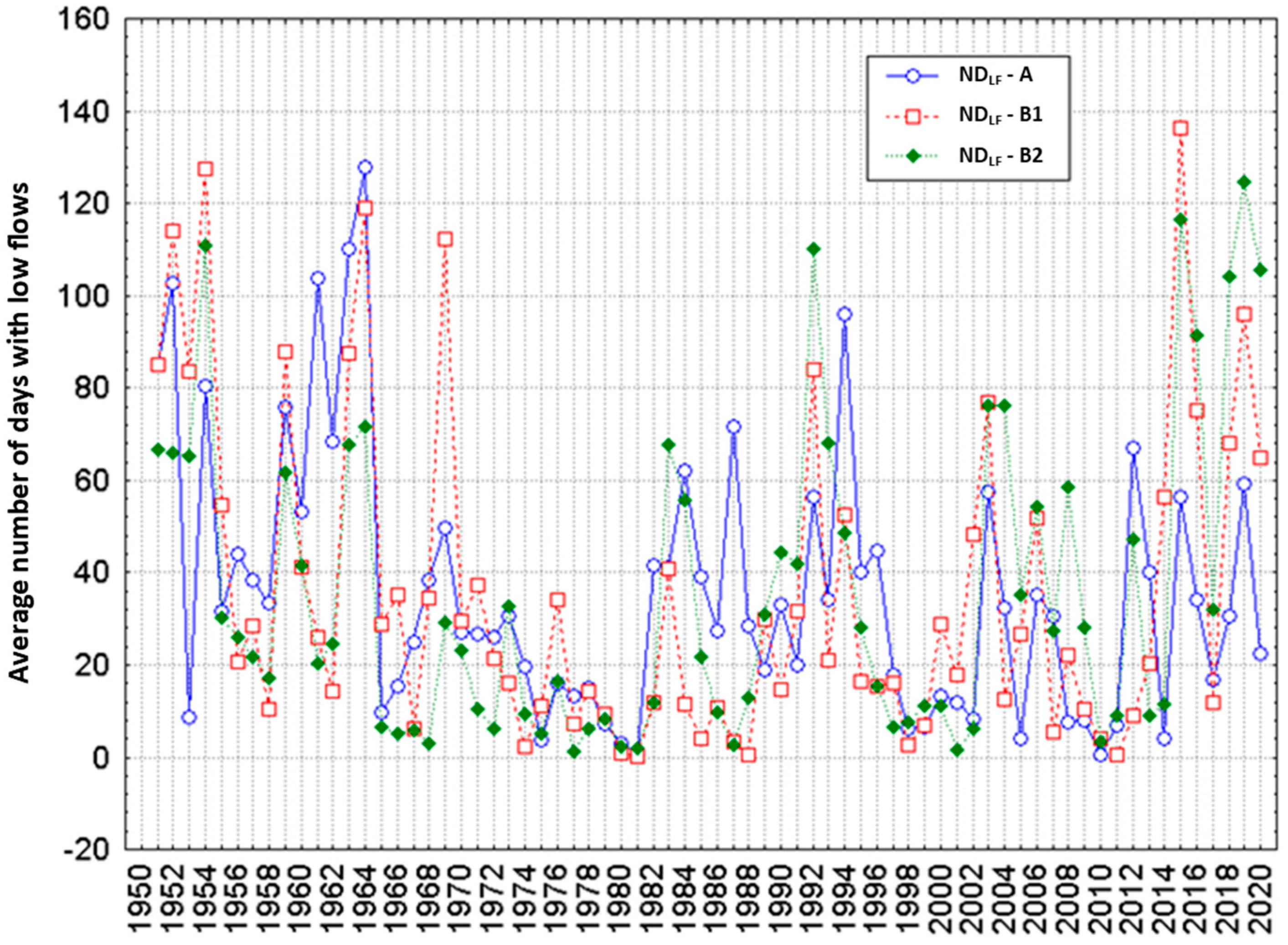
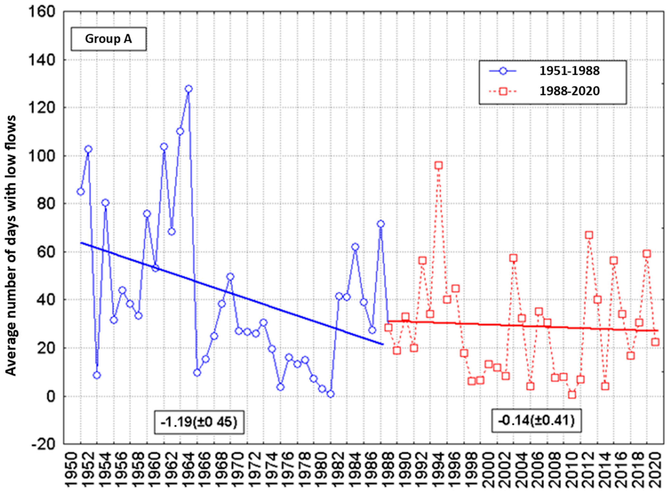
• The grouping of water gauges based on the ND_LF revealed its regional differentiation. This led to a separation of two groups of gauges forming relatively homogenous territorial groups spatially. The distinguished group A included the south-eastern part of Poland, while group B covered the remaining part of the country. Group B was additionally split into sub-group B1 covering Northern and North-eastern Poland and sub-group B2 covering the south-western part of the country. The most important reason for the formation of these separate types in the ND_LF set was differences in the nature of the variability of the course of the ND_LF. The analysis of linear trends in each of the areas, carried out in each area separately for the years 1951–1988 and for the years 1988–2020, i.e., in the sub-periods before and after climate change, revealed the basic difference in their course between group A and sub-groups B1 and B2.

The presented results for the whole analyzed period (1951–2020) are in line with findings of [22]. The authors, using the trend decomposition method, showed that duration time of streamflow droughts (in the period 1965–2020) decreased in the south-eastern part of the Vistula basin and increased in most of other river gauges in Poland.

The proposed method has some limitations. It concerns ND_LF as only one parameter of low flows referring to the total time of occurrence of the phenomenon in a given year, while low flows can be described by parameters linked to factors, such as drought/low flow severity (like volume or minimal flow) or the number of episodes. In future research, the threshold method used to select low flow events could be reconsidered as the problem of the objectivity of the choice of thresholds values has been raised by [46].

Our research also focuses on changing climate conditions and their impact on low flows. The specific changes in precipitation and evaporation in 1951–1988 and 1988–2020 resulted in the formation of three spatially homogenous areas in Poland (marked as A, B1, and B2) differing in the course of the climatic water balance and trends in the course of ND_LF over time. However, in some of the analyzed river gauges, the anthropogenic influence (such as land use changes, water management practices, or water intake) may play a key role in explaining the observed trends in low flow changes.

To sum up, low flows research and understanding of their changes under climate warming conditions are crucial for developing proper and responsible water management practices, taking into account their impact on aquatic ecosystems, biodiversity, and economic activity (especially agriculture). Our research results show that policymakers should consider developing proper water management and drought consequences mitigation strategies and plans focusing on different objectives for each identified region.

References

1. Döll, P.; Jiménez-Cisneros, B.; Oki, T.; Arnell, N.W.; Benito, G.; Cogley, J.G.; Jiang, T.; Kundzewicz, Z.W.; Mwakalila, S.; Nishijima, A. Integrating risks of climate change into water management. Hydrol. Sci. J. 2015, 60, 4–13. [Google Scholar] [CrossRef]
2. Marshall, A.; Grubert, E.; Warix, S. Temperature Overshoot Would Have Lasting Impacts on Hydrology and Water Resources. Water Resour. Res. 2025, 61, e2024WR037950. [Google Scholar] [CrossRef]
3. Kundzewicz, Z.W. Climate Change Impacts on the Hydrological Cycle. Ecohydrol. Hydrobiol. 2008, 8, 195–203. [Google Scholar] [CrossRef]
4. Ciampittiello, M.; Marchetto, A.; Boggero, A. Water Resources Management under Climate Change: A Review. Sustainability 2024, 16, 3590. [Google Scholar] [CrossRef]
5. Wrzesiński, D. Changes in selected characteristics of river regime in Poland under climate warming conditions. Acta Geogr. Lodz. 2024, 115, 175–195. (In Polish) [Google Scholar] [CrossRef]
6. Schneider, C.; Laizé, C.L.R.; Acreman, M.C.; Flörke, M. How Will Climate Change Modify River Flow Regimes in Europe? Hydrol. Earth Syst. Sci. 2013, 17, 325–339. [Google Scholar] [CrossRef]
7. Bartczak, A.; Krzemiński, M.; Araźny, A. Changes in Evaporation Patterns and Their Impact on Climatic Water Balance and River Discharges in Central Poland, 1961–2020. Reg. Environ. Change 2024, 24, 130. [Google Scholar] [CrossRef]
8. Pińskwar, I.; Choryński, A.; Graczyk, D.; Kundzewicz, Z.W. Observed Changes in Precipitation Totals in Poland. Geografie 2019, 124, 237–264. [Google Scholar] [CrossRef]
9. Szwed, M. Variability of Precipitation in Poland under Climate Change. Theor. Appl. Climatol. 2019, 135, 1003–1015. [Google Scholar] [CrossRef]
10. Wibig, J.; Jędruszkiewicz, J. Recent Changes in the Snow Cover Characteristics in Poland. Int. J. Clim. 2023, 43, 6925–6938. [Google Scholar] [CrossRef]
11. Pińskwar, I.; Choryński, A.; Graczyk, D.; Kundzewicz, Z.W. Observed Changes in Extreme Precipitation in Poland: 1991–2015 versus 1961–1990. Theor. Appl. Climatol. 2019, 135, 773–787. [Google Scholar] [CrossRef]
12. Łupikasza, E.B.; Małarzewski, Ł. Trends in the Indices of Precipitation Phases under Current Warming in Poland, 1966–2020. Adv. Clim. Change Res. 2023, 14, 97–115. [Google Scholar] [CrossRef]
13. Somorowska, U. Assessing the Impact of Climate Change on Snowfall Conditions in Poland Based on the Snow Fraction Sensitivity Index. Resources 2024, 13, 60. [Google Scholar] [CrossRef]
14. Wibig, J.; Jędruszkiewicz, J. Are Heatwaves and Drought More Likely to Occur Simultaneously with Warming? EMS Annu. Meet. Abstr. 2023, 20, EMS2023-329. [Google Scholar] [CrossRef]
15. Zhu, S.; Luo, Y.; Graf, R.; Wrzesiński, D.; Sojka, M.; Sun, B.; Kong, L.; Ji, Q.; Luo, W. Reconstruction of Long-Term Water Temperature Indicates Significant Warming in Polish Rivers during 1966–2020. J. Hydrol. Reg. Stud. 2022, 44, 101281. [Google Scholar] [CrossRef]
16. Sun, J.; Nunno, F.D.; Sojka, M.; Ptak, M.; Zhou, Q.; Luo, Y.; Zhu, S.; Granata, F. Long-Term Daily Water Temperatures Unveil Escalating Water Warming and Intensifying Heatwaves in the Odra River Basin, Central Europe. Geosci. Front. 2024, 15, 101916. [Google Scholar] [CrossRef]
17. Zhou, Q.; Nunno, F.D.; Sun, J.; Sojka, M.; Ptak, M.; Qian, J.; Zhu, S.; Granata, F. Characteristics of River Heatwaves in the Vistula River Basin, Europe. Heliyon 2024, 10, e35987. [Google Scholar] [CrossRef] [PubMed]
18. Ptak, M.; Olowoyeye, T.; Sojka, M. Trends of Changes in Minimum Lake Water Temperature in Poland. Appl. Sci. 2022, 12, 12601. [Google Scholar] [CrossRef]
19. Olowoyeye, T.; Ptak, M.; Sojka, M. How Do Extreme Lake Water Temperatures in Poland Respond to Climate Change? Resources 2023, 12, 107. [Google Scholar] [CrossRef]
20. Raczyński, K.; Dyer, J. Changes in Streamflow Drought and Flood Distribution over Poland Using Trend Decomposition. Acta Geophys. 2024, 72, 2773–2794. [Google Scholar] [CrossRef]
21. Forzieri, G.; Feyen, L.; Rojas, R.; Flörke, M.; Wimmer, F.; Bianchi, A. Ensemble Projections of Future Streamflow Droughts in Europe. Hydrol. Earth Syst. Sci. 2014, 18, 85–108. [Google Scholar] [CrossRef]
22. Piniewski, M.; Szcześniak, M.; Kundzewicz, Z.W.; Mezghani, A.; Hov, Ø. Changes in Low and High Flows in the Vistula and the Odra Basins: Model Projections in the European-scale Context. Hydrol. Process. 2017, 31, 2210–2225. [Google Scholar] [CrossRef]
23. Kundzewicz, Z.W.; Piniewski, M.; Mezghani, A.; Okruszko, T.; Pińskwar, I.; Kardel, I.; Hov, Ø.; Szcześniak, M.; Szwed, M.; Benestad, R.E.; et al. Assessment of Climate Change and Associated Impact on Selected Sectors in Poland. Acta Geophys. 2018, 66, 1509–1523. [Google Scholar] [CrossRef]
24. Wrzesiński, D.; Marsz, A.A.; Sobkowiak, L.; Styszyńska, A. Response of Low Flows of Polish Rivers to Climate Change in 1987–1989. Water 2022, 14, 2780. [Google Scholar] [CrossRef]
25. Lorenc, H. Climatological and meteorological extremes in Poland in relation to the 5th IPCC Report. In Klimat a Społeczeństwo i Gospodarka; Lorenc, H., Ustrnul, Z., Eds.; Wyd. PT Geofizyczne i IMGW-PIB: Warsaw, Poland, 2015; pp. 31–51. (In Polish) [Google Scholar]
26. Marsz, A.A.; Sobkowiak, L.; Styszyńska, A.; Wrzesiński, D. Causes and Course of Climate Change and Its Hydrological Consequences in the Greater Poland Region in 1951–2020. Quaest. Geogr. 2022, 41, 183–206. [Google Scholar] [CrossRef]
27. Sutton, R.T.; Hodson, D.L.R. Atlantic Ocean forcing of North American and European summer climate. Science 2005, 309, 115–118. [Google Scholar] [CrossRef]
28. Sutton, R.T.; Dong, B. Atlantic Ocean influence on a shift in European climate in the 1990s. Nat. Geosci. 2012, 5, 788–792. [Google Scholar] [CrossRef]
29. Wrzesiński, D.; Marsz, A.; Styszyńska, A.; Sobkowiak, L. Effect of the North Atlantic Thermohaline Circulation in Changes in Climate Conditions and River Flow in Poland. Water 2019, 11, 1622. [Google Scholar] [CrossRef]
30. Pociask-Karteczka, J.; Limanówka, D.; Nieckarz, Z. Impact of North Atlantic oscillation on the flows of the Carpathian rivers (1951–2000). Folia Geogr. Ser. Geogr. Phys. 2003, 33–34, 89–104. (In Polish) [Google Scholar]
31. Pociask-Karteczka, J. River runoff response to climate changes in Poland (East-Central Europe). In Hydro-Climatology: Variability and Change (Proceedings of Symposium J-H02 Held During IUGG 2011 in Melbourne, Australia, July 2011); IAHS Publ.: Maastricht, The Netherlands, 2011; Volume 344. [Google Scholar]
32. Piniewski, M.; Laizé, C.L.; Acreman, M.C.; Okruszko, T.; Schneider, C. Effect of climate change on environmental flow indicators in the Narew Basin, Poland. J. Environ. Qual. 2014, 43, 155–167. [Google Scholar] [CrossRef] [PubMed]
33. Malinowski, Ł.; Skoczko, I. Impacts of Climate Change on Hydrological Regime and Water Resources Management of the Narew River in Poland. J. Ecol. Eng. 2018, 19, 4. [Google Scholar] [CrossRef]
34. Gizińska, J.; Sojka, M. How Climate Change Affects River and Lake Water Temperature in Central-West Poland—A Case Study of the Warta River Catchment. Atmosphere 2023, 14, 330. [Google Scholar] [CrossRef]
35. Okołowicz, W. General Climatology; Wydawnictwo Naukowe PWN: Warsaw, Poland, 1976; pp. 1–422. (In Polish) [Google Scholar]
36. Kędziora, A. Fundamentals of Agro-Meteorology; Państwowe Wydawnictwo Rolnicze i Leśne: Warsaw, Poland, 1999; pp. 1–364. (In Polish) [Google Scholar]
37. Kędziora, A. Water balance of Konin strip mine landscape in changing climatic conditions. Rocz. Glebozn. 2008, 59, 104–118. (In Polish) [Google Scholar]
38. Radzka, E. Climatic water balance for the vegetation season (according to Ivanov’s equation) in Central-Eastern Poland. Woda-Środowisko-Obsz. Wiej. 2014, 14, 67–76. (In Polish) [Google Scholar]
39. Okoniewska, M.; Szumińska, D. Changes in Potential Evaporation in the Years 1952–2018 in North-Western Poland in Termsof the Impact of Climatic Changes on Hydrological an Hydrochemical Condotions. Water 2020, 12, 877. [Google Scholar] [CrossRef]
40. Raczyński, K.; Dyer, J. Development of an Objective Low Flow Identification Method Using Breakpoint Analysis. Water 2022, 14, 2212. [Google Scholar] [CrossRef]
41. Stahl, K.; Vidal, J.-P.; Hannaford, J.; Tijdeman, E.; Laaha, G.; Gauster, T.; Tallaksen, L.M. The Challenges of Hydrological Drought Definition, Quantification and Communication: An Interdisciplinary Perspective. Proc. Int. Assoc. Hydrol. Sci. 2020, 383, 291–295. [Google Scholar] [CrossRef]
42. Ward, J.H. Hierarchical Grouping to Optimize an Objective Function. J. Am. Stat. Assoc. 1963, 58, 236–244. [Google Scholar] [CrossRef]
43. Grabiński, T.; Wydymus, S.; Zeliaś, A. Numerical Taxonomy Methods in Modeling Socio-Economic Phenomena; Wydawnictwo Naukowe PWN: Warsaw, Poland, 1989; pp. 1–278. (In Polish) [Google Scholar]
44. Mojena, R. Hierarchical grouping methods and stopping rules: An evaluation. Comput. J. 1977, 20, 359–363. [Google Scholar] [CrossRef]
45. Rotnicka, J. Typology of Hydrological Periods for Use in River Regime Studies. Quaest. Geogr. 1993, 15/16, 77–95. [Google Scholar]
46. Milligan, G.W.; Cooper, M.C. An examination of procedures for determining the number of clusters in a data set. Psychometrika 1985, 50, 159–179. [Google Scholar] [CrossRef]
47. Marsz, A.A.; Styszyńska, A.; Bryś, K.; Bryś, T. Role of internal variability in climate system in increase of air temperature in Wrocław (Poland) in the years 1951–2018. Quaest. Geogr. 2021, 40, 109–124. [Google Scholar] [CrossRef]
48. Wrzesiński, D. Flow Regime Patterns and Their Changes. In Management of Water Resources in Poland; Zeleňáková, M., Kubiak-Wójcicka, K., Negm, A.M., Eds.; Springer: New York, NY, USA, 2021; pp. 163–180. [Google Scholar] [CrossRef]
Figure 1. Geographical positions of meteorological stations and water gauges in the study area. Numbering was performed in accordance with Table A1.
Water 17 00243 g001
Figure 2. The average values of hydro-meteorological elements ((A) temperature; (B) precipitation; (C) evaporation; (D) runoff) and trends of their changes in the multi-annual period 1951–2020.
Water 17 00243 g002
Figure 3. Changes in the average values of hydro-meteorological elements ((A) temperature; (B) precipitation; (C) evaporation; (D) runoff) in the warming period after 1988 compared to in the period 1951–1988 and their statistical significance.
Water 17 00243 g003
Figure 4. The average numbers of NDLF days and their trends in the multi-annual period 1951–2020 and the two sub-periods before and after climate warming.
Water 17 00243 g004
Figure 5. Correlations between annual NDLF and air temperature (A), evaporation (B), and precipitation amount (C) and their statistical significance (p).
Water 17 00243 g005
Figure 6. Dendrogram of water gauge grouping due to NDLF (Q = 0.1) in subsequent years of the multi-annual period 1951–2020 with a graph of the linkage distance curve. Numbering was performed in accordance with Appendix A.
Water 17 00243 g006
Figure 7. The course of the number of days with low flows in a year in individual groups.
Water 17 00243 g007
Figure 8. The geographical positions of water gauges in groups distinguished with the use of Ward’s hierarchical grouping method against the background of changes in the average NDLF in the hydrological year in the warming period after 1988 compared to in the period 1951–1988.
Water 17 00243 g008
Figure 9. The course of the area-averaged number of days with low flows per year (NDLF) in SE Poland (group A) with linear trends in the years 1951–1988 and 1988–2020 (days per year). Trend values and standard errors of their estimation (in brackets, following the trend value) are shown in frames.
Water 17 00243 g009
Figure 10. The course of the area-averaged number of days with low flows per year (NDLF) in N and NE Poland (group B1) with linear trends in the years 1951–1988 and 1988–2020 (days per year). Trend values and standard errors of their estimation (in brackets, following the trend value) are shown in frames.
Water 17 00243 g010
Figure 11. The course of the area-averaged number of days with low flows per year (NDLF) in W and SW Poland (group B2) with linear trends in the years 1951–1988 and 1988–2020 (days per year). Trend values and standard errors of their estimation (in brackets, following the trend value) are shown in frames.
Water 17 00243 g011
Figure 12. Changes of the correlation coefficients between NDLF and air temperature (T), precipitation (P), and evaporation (Ev) in subsequent 20-year periods of the multi-annual period 1951–2020 in three distinguished groups.
Water 17 00243 g012