Multi-Objective Optimal Planning and Deciding of Low Impact Development for an Intending Urban Area

Abstract

As a storm management philosophy, low impact development (LID) is used to control the surface flow and its pollution, especially in the intending urban area in China. Finding the proper LID plan to balance the cost and surface flow effect is very important for the administrators of the cities. Firstly, we combined the SWMM with NSGA II to find the Pareto set of these optimal LID plans. Then, a structural decision-making approach was used to select the proper scheme from the Pareto set. The numerical tests consisted of 40 combinations of different return periods and durations and were conducted. The result shows that the SWMM-NSGA II model is a distributed model which could be used to find the multi-objective optimization LID plans for an intending urban area. When the SDA is used to select the suitable scheme from the Pareto set composed by the optimal alternatives, the weights could reflect the management demand of people. The LIDs might be more effective for more frequent, lighter, and shorter duration storms. It could cost too much, but the control effective might not be obvious in a heavy storm.

1. Introduction

Urbanization has modified the land surface greatly by reducing vegetative cover and increasing impervious urban watersheds. It has led to precipitation infiltration decrease and converts runoff which could impact both the quantity and quality of urban runoff [1]. There are many storm water management conceptions, such as low impact development (LID) [2], best management practices (BMPs) [3], sustainable urban drainage system (SUDS) [4], green infrastructures (GIs) [5], and water sensitive urban design (WSUD) [6]. These conceptions have been considered as efficient protection ways for water quality, flood detention, and ecology protection in urban areas. The LID conception has been implemented in many metropolises of China to control runoff and pollution [7,8]. The Chinese government has promoted the sponge city conception in urbanization to manage the storm water since 2010. Many laws and theories are established to guide the storm water management [9,10], and many researchers contribute a lot of effort to improve LID facilities [11]. The proper prediction of urban runoff quantity and quality in to-be-developed areas is essential for preventing city flooding, reducing storm water pollution, and deciding city planning.

Computer modeling is helpful to understand the current and future impact of land use changes on urban water bodies, and it could be used to design and optimize storm water management [12,13,14]. Bosley (2008) gives an in-depth review of the common models [15]. The hydrological process in LID controls are analyzed by many researchers with computer models [13]. In addition to the assessment of common hydrological processes, climatic changes, biological process, chemical process, and uncertainties in decision-making are also considered in recent studies of storm management. Wang et al. (2019) assessed the hydrological effects of bioretention cells to control urban storm water runoff. Considering the climatic changes in a hypothetical urban catchment [16], they examined the first flush with different storm management designs using the SWMM. Silva et al. (2019) analyzed the impact of urban storm water runoff on cyanobacteria dynamics in Lake Pampulha located in Belo Horizonte, Brazil [17]. Rezaei et al. (2019) used the SWMM and collected field data to assess the impacts of LIDs on water quality and hydrology at the catchment scale in Kuala Lumpur, Malaysia [18]. Raei et al. (2019) proposed a decision-making framework for GI planning to control urban storm water management considering various uncertainty [14]; they combined a fuzzy multi-objective model and a surrogate model based on the calibrated SWMM to reduce the runtime.

The decision-making process of urban area low impact development is complicated because it could relate to multiple objectives of runoff control, such as volume reduction, water quality improvement, and LID cost-effectiveness. Some researchers tried to find an optimization scheme for the multi-objective problem using a multi-objective optimization technique combined with the hydrology model, the water quality model, cost-effectiveness analysis, and an optimization algorithm [19,20,21]. Due to open-source features, robustness, and a low impact development (LID) module, the SWMM is commonly used and coupled with optimization algorithms [22]. Optimization tools such as genetic algorithm (GA) [23], a technique to order preference by similarity to an ideal solution (TOPSIS) [24], particle swarm optimization (PSO) [25], and simulated annealing (SA) [26] were combined with SWMM to find the optimization scheme for urban drainage planning and design. As a popular tool, the non-dominated sorting genetic algorithm II (NSGA-II) [27] has been widely used for solving multi-objective optimization problems, and it is very efficient for multi-objective optimization studies [28]. Zare et al. (2012) used NSGA-II to set up a multi-objective optimization model for combined quality–quantity urban runoff control [29]. Raei et al. (2019) [14] combined the NSGA-II and fuzzy α-cut technique to form a fuzzy optimization approach. Macro et al. (2019) connected the SWMM with the existing Optimization Software Toolkit for Research Involving Computational Heuristics (OSTRICH) to reduce the combined sewer overflows for the city of Buffalo, New York, USA [30]. With the help of these heuristic optimization algorithms, the Pareto front is composed of large amounts of optimal LID schemes and could be given to decision makers. Though all these schemes are theoretically optimal solutions, it is difficulty for decision makers to choose the proper LID scheme based on their purpose. Almost all these multi-objective optimization techniques focus on finding the whole schemes of Pareto front for decision makers, but few studies bring a convenient method for decision makers to select suitable schemes from a huge group of multi-objective optimization results.

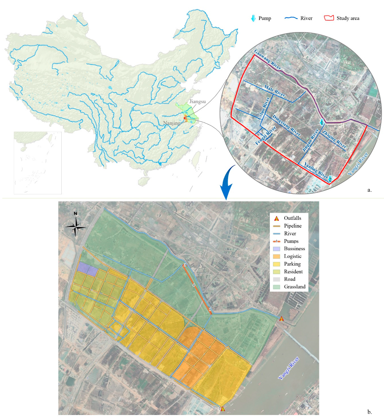
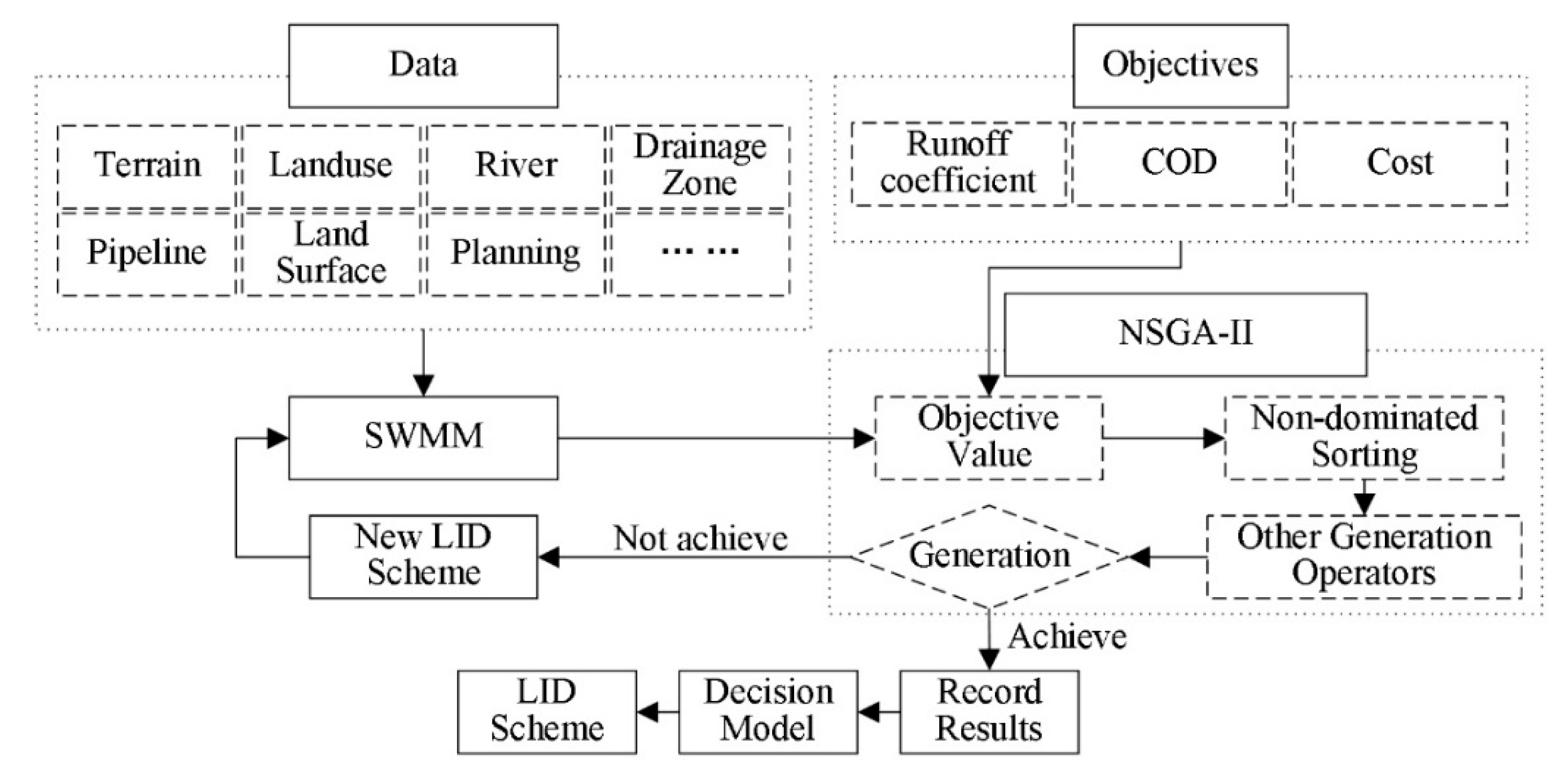
The main objective of this study is to provide a method to find proper optimal LID planning alternatives from a large number of multi-objective optimization results by combining a decision-making algorithm with an integrated SWMM-NSGA II model. The SWMM model is used to simulate the hydrological, hydraulic, and water quality processes of the area under different LID scenarios. Then, it is integrated into the NSGA II to construct a SWMM-NSGA II model to find the multi-objective optimization LID plans. Finally, the structural decision-making approach for multi-objective system [31] is combined with the SWMM-NSGA II to identify proper optimal LID planning alternatives from the multi-objective optimization results. The proposed framework was applied to an intending urban area in Nanjing. It was used to ensure maximum chemical oxygen demand (COD) load reduction, maximum runoff reduction, and minimum total relative cost.

2. Study Site

The study area is about 14.7 km² in size and is located west of Nanjing, Jiangsu Province (Figure 1a). At present, it is used for agricultural purposes. According to the city planning, the whole study area will become an urban area and will be covered by roads and modern buildings by 2025 (Figure 1b). The Yangzi River flows through the east of the area. The north border of the area is Gaowang River which flows into the Yangzi River from the east. The west and south of the area are surrounded by urban expressways. The whole study area could be taken as a completed drainage system, and all the water flows into or out of the area through rivers, pipelines, and pumps (Figure 1b). There are ten small rivers in the study area. The storm water and surface runoff are mainly conveyed by these rivers, and the water is finally pumped out of the area via two pump stations. The terrain is flat, so the water in the rivers is almost still. To make water flow in the local circulation, pump station 4 is going to be constructed to transport water from Jinpan River to Male River. The north part of the area consists of unused land and is covered by grass. The south part of the area is for logistic and parking purposes with a few resident and business blocks. Urbanization might reduce rainfall infiltration and increase surface runoff. The rivers might be contaminated with pollutants carried by surface runoff. Therefore, a proper LID plan is needed to alleviate surface runoff and water pollution.

3. Methods

In this paper, the SWMM model is set up to simulate the hydrological, hydraulic, and water quality processes of the area and analyze different LID scenarios, and it is also integrated into the NSGA II to construct a SWMM-NSGA II model to find the multi-objective optimization LID plans. The structural decision fuzzy set theory [31] is used to identify proper optimal LID planning alternatives from the multi-objective optimization results. Figure 2 shows the process to find the proper LID scheme.

3.1. Hydraulic, Hydrologic, and Quality Modeling

In this study, EPA SWMM 5.1.012 is used to simulate the hydrologic, hydraulic, and quality processes as well as the performance of LIDs. Since it is suited to simulate runoff quantity and quality from primarily urban areas [32], it can simulate the hydrologic performance of LID infrastructures [33]. More importantly, it is a robust model with open-source codes which could be conveniently combined with the optimization algorithm.

3.1.1. Hydraulic and Hydrologic Model

The dynamic wave method is used to perform flood routing. It could simulate channel storage, entrance/exit losses, flow reversal, backwater effects, and pressurized flow [34].

The study area is subdivided into 175 subcatchments according to the city planning. Horton’s equation [35] is used to analyze the infiltration losses. The input parameters of this method include the maximum and minimum infiltration rates, a decay coefficient that describes how fast the rate decreases over time, and the time it takes fully saturated soil to completely dry (used to compute the recovery of infiltration rate during dry periods).

The study area will become an urban area in the future. The land surface, river cross-sections, and the flow dynamics will change a lot. We want to find the proper optimal LID schemes based on the city planning, but we have no data for calibration and validation. The comprehensive runoff coefficient (CRC) method [36] is used to calibrate and validate the parameter values. Firstly, the initial parameter values were decided according to the sponge city guidance [9] and the city planning [36,37]; then, the SWMM model with these parameters was ran to obtain the simulated CRC. If the simulated CRC falls within the requirement range of corresponding empirical CRC [9], then the final parameters were taken as the final parameters, otherwise the input parameters were modified until the simulated CRC fell within the range of the corresponding CRC. All the simulated CRCs satisfied the requirement range of the empirical CRC (

Table 1. Land use percent and the comprehensive runoff coefficient (CRC) of the study area.

Land Use	Percent of the Study Area	Empirical CRC	Simulated CRC
Business	0.94%	0.85~0.95	0.94
Resident	8.95%	0.85~0.95	0.95
Road	12.12%	0.85~0.95	0.95
Logistic	8.10%	0.85~0.95	0.92
Parking	28.10%	0.40~0.50	0.48
Grassland	41.79%	0.10~0.20	0.13

). The final parameters are shown

Table 2. The surface parameters of different land use.

Land Use	Business	Resident	Road	Logistic	Parking	Grassland
Percent of impervious area	55%	30–60%	95%	40–65%	55–70%	10%
Manning’s n for impervious area	0.013	0.02	0.013	0.015	0.024	0.012
Manning’s n for pervious area	0.13	0.05	0.05	0.05	0.05	0.14
Depth of depression storage on impervious area (mm)	1.25	1.25	1.25	1.25	1.25	1.25
Depth of depression storage on pervious area (mm)	5	5	5	3	3	5

,

Table 3. The Horton equation’s parameters of previous area of different land use.

Land Use	Max. Infiltration (mm/h)	Min. Infiltration (mm)	Decay Coefficient (1/h)	Drying Time (Day)
Business	50	7.6	4	7
Resident	50	7.6	4	7
Road	22	7.6	4	7
Logistic	22	7.6	4	7
Parking	22	7.6	4	7
Grassland	78	16	4	7

and

Table 4. The Manning’s roughness coefficient of rivers and pipelines.

Conduits	Manning’s Roughness Coefficient
River	0.07
Pipeline	0.012

. The empirical CRC and the parameters of different land use are not very definite values, so sensitivity and uncertainty might affect the SWMM model and the LID schemes. To maintain a more reliable model, many researchers provide a lot of effort to discover the uncertainty, but we just focus on the whole framework to find the optimal LID schemes by identifying the proper one in this work. Sensitivity and uncertainty should be discussed in detail in future studies.

3.1.2. Wash-Off Model

Through the surface wash-off effect, the pollutants will be carried to the river by surface runoff. Though there are several approaches to evaluate wash-off [37], SWMM incorporates three different choices of empirical models to describe pollutant wash-off: event mean concentration (EMC) wash-off, exponential wash-off, and rating curve wash-off [33]. The EMCs are the most common parameters used to estimate nonpoint water quality loads in SWMM [33], so we use the EMCs to describe the wash-off load. In this study, the chemical oxygen demand (COD) is taken as the typical pollutant.

Because future EMC of COD is not available, the water quality calibration process for COD concentration is impossible. According to the relevant studies [38,39,40], the EMC could range from 20 mg/L to 600 mg/L in different land use.

3.1.3. Selection of the LIDs

The south part of the area is for logistic and parking purposes. There are a few resident and business blocks in the area. The logistic sites, buildings, and roads contribute to most of the impervious area, which might lead to more surface runoff and pollution. Rain gardens and continuous porous pavements are beneficial for both residential and commercial settings [41], and vegetative swale could reduce storm water volumes and pollution loads into rivers and lakes [42], so we choose rain garden, permeable pavement, and vegetative swale for the study area.

Continuous porous pavement systems (CPPs) are excavated areas filled with gravel and paved over with porous concrete or asphalt mix (Figure 3a) [43]. Rainfall could fall on the surface and pass through the pavement into the gravel storage layer, and it can infiltrate into the site’s native soil. A rain garden (RG), also called a storm water garden [44], is designed as a depression storage or a planted hole that allows rainwater runoff from impervious urban areas, like roofs, driveways, walkways, parking lots, and compacted lawn areas, the opportunity to be absorbed (Figure 3b). Rain and runoff could come into the surface layer, some could infiltrate into the soil layer, and others might go out of the rain garden. Vegetative swales (VSs) are channels or depressed areas with sloping sides covered with grass and other vegetation (Figure 3c). They slow down the conveyance of collected runoff and allow it more time to infiltrate into the native soil [33]. The parameters of the CPPs, RG, and VSs are given by the city planning [36,37] (

Table 5. Parameters of the continuous porous pavement.

Layer	Parameter	Value
Surface layer	Manning’s n	0.1
	Slope	1.0
Pavement layer	Thickness (mm)	150.0
	Void ratio	0.2
	Impervious surface	0.0
	Permeability (mm/h)	100.0
Storage layer	Thickness (mm)	200.0
	Void ratio	0.75
	Seepage rate (mm/h)	3.6

,

Table 6. Parameters of the rain garden.

Layer	Parameter	Value
Surface layer	Berm height (mm)	150.0
	Vegetation volume	0.05
	Manning’s n	0.16
	Slope	1.0
Soil layer	Thickness (mm)	500.0
	Porosity	0.3
	Field capacity	0.2
	Wilting point	0.1
	Conductivity (mm/h)	20.0
	Conductivity slope	10.0
	Suction head (mm)	3.5

and

Table 7. Parameters of the vegetative swales.

Layer	Parameter	Value
Surface layer	Berm height (mm)	150.0
	Vegetation volume	0.1
	Manning’s n	0.12
	Slope	5.0

).

3.2. Optimization Model and Algrithm

The objectives of the optimization problem were to (1) minimize the total relative cost of LID implementation, (2) minimize the runoff coefficient of the study area, and (3) minimize the pollutant concentration of the study area. The decision variables were defined as the area of LIDs of each subcatchment in the study area. There might be several types of LID in the same subcatchment. For each applicable LID type, the decision variable should not be negative. The sum of the area of each applicable LID type should be smaller than the total impervious area of the corresponded subcatchment. Mathematically, the optimization problem can be expressed as follows:

$$F_1=\min {\sum }_{\begin{array}{c}0\le i\le n\\ 0<j<m\end{array}}{x}_{ij}{A}_{ij},$$

(1)

$$F_2=\min {\sum }_{i=1}^n{\displaystyle \frac{r_i}{R_i}},$$

(2)

$$F_3=\min {\sum }_{i=1}^n{\displaystyle \frac{c_i}{C_i}},$$

(3)

where the $x_{ij}$ is the LID cost per unit area of the $j$-th LID infrastructure in the $i$-th subcatchment (CNY/m²). Ren et al. (2017) have investigated the LID cost in China [45], and their research was used in this paper. The $A_{ij}$ is the area of the $j$-th LID infrastructure in the $i$-th subcatchment; the $r_i$ is the evaluated runoff coefficient of the $i$-th subcatchment; the $R_i$ is the aim runoff coefficient of the $i$-th subcatchment. The $c_i$ is the evaluated pollutant concentration of the $i$-th subcatchment; the $C_i$ is the aim pollutant concentration of the $i$-th subcatchment. $R_i$ is 0.7, and the $C_i$ is 40 mg/L in this study. If there is no specific control aims for the runoff and pollutant concentrations, both $R_i$ and $C_i$ are set as 1. We could set specific $R_i$ and $C_i$ values for each subcatchment depending on the particular aim.

The NSGA-II is one of the promising multi-objective evolutionary algorithms that could provide optimal or near optimal trade-off solutions among competing objectives [27]. As an improved version of the NSGA [46], the NSGA-II is developed to address issues of computational complexity as well as to provide an explicit mechanism for diversity preservation. A non-dominating sorting approach is incorporated to make it faster than any other multi-objective algorithm. The algorithm consists of five operators: initialization, fast non-dominated sorting, crossover, mutation, and the elitist crowded comparison operator. In recent years, the NSGA-II has shown superiority over other multi-objective evolutionary algorithms in solving LID optimization problems [14,29,47,48].

3.3. Method for Decision-Making

The structural decision-making approach for the multi-objective system (SDA) could provide help for selecting a suitable scheme from the Pareto set that is composed of optimal alternatives [31].

When the SWMM-NSGA II gives $n$ schemes, the decision makers would find the most suitable scheme from them according to the $m$ objective eigenvalues. The superior and inferior concepts are relative concepts, so we first grade the suitability of the schemes into $c$ categories with a relative membership degree of fuzzy mathematics. It describes how close a scheme belongs to the superior concept. The relative membership degree of the superior category to the fuzzy superior concept is defined as 1, and the value for inferior category is 0. It is assumed that it changes linearly from the superior to inferior. The stand value vector of relative membership degree $s_{ih}$ for all the $c$ categories is described as follows:

$$s_{ih}=\left(1,{\displaystyle \frac{c-2}{c-1}},{\displaystyle \frac{c-3}{c-1}},\cdots ,0\right),\forall i,h=1,2,\cdots ,c,$$

(4)

Then, we can calculate the matrix of relative membership degrees. If the smaller value of objective is better, the matrix of relative membership degrees in this study are described as follows:

$$R=\left(r_{ij}\right),i=1,2,\cdots ,m,j=1,2,\cdots ,n,$$

(5)

$$r_{ij}=\left(\underset{j}{\max }{x}_{ij}-x_{ij}\right)/\left(\underset{j}{\max }{x}_{ij}-\underset{j}{\min }{x}_{ij}\right),$$

(6)

where $x_{ij}$ is the element of the scheme objective eigenvalue matrix, and $r_{ij}$ is the relative membership degree of scheme $j$ to objective $i$.

Comparing $r_{ij}$ with $s_{ih}$, we could find the interval where the $r_{ij}$ falls in the $s_{ih}$, denoted as $\left[a_{ij},b_{ij}\right]$. Then, we could obtain the upper limit and the lower limit corresponding to scheme $j$ as follows:

$$a_j=\underset{i}{\min }{a}_{ij},b_j=\underset{i}{\max }{b}_{ij},$$

(7)

It is a complex decision to identify the schemes of constructing urban infrastructures because many benefits and goal need to be satisfied. The weight of these goals are induced to distinguish their importance.

In this study, we used two steps to decide the weight of the objectives. Firstly, the entropy weight method could provide the objective appraisal for the weight [49], if there are many objectives. The entropy weight vector could be described as follows:

$$W=\left(w_i\right),w_i={\displaystyle \frac{1-E_i}{m-\sum _{i=1}^m{E}_i}},$$

(8)

$$E_i=-{\displaystyle \frac{1}{\ln \left(n\right)}}\left({\sum }_{j=1}^n{f}_{ij}\ln \left(f_{ij}\right)\right),f_{ij}={\displaystyle \frac{1+r_{ij}}{\sum _{j=1}^n\left(1+r_{ij}\right)}},i=1,2,\cdots ,m,j=1,2,\cdots ,n,$$

(9)

The entropy weights are deduced based on the data set of the objectives and are calculated using NSGA II. They are totally objective and cannot reflect the subjective demand of the public in an urban area. But the will and feelings of the people should be considered as an important factor when the LIDs or other urban infrastructures are constructed. The entropy weights could be taken as the references; then, the weight could be adjusted based on the experiences and knowledge of the storm water manager. For example, if the managers want to reduce more pollutants in the runoff, the weight of the third objective should be artificially increased. But we must notice that the adjusted weights should be normalized to ensure the sum of the weight equals 1. If there are a few objectives, the weight could also be directly decided by the manager.

With these weights, we could describe the relative membership matrix with the following equations:

$$U=\left(u_{hi}\right),j=1,2,\cdots ,n,h=1,2,\cdots ,c,$$

(10)

$$u_{hj}=\left\{\begin{array}{cc}0& h<a_{j}orh>b_j\\ {\displaystyle \frac{1}{\sum _{k=a_j}^{b_j}\left\{\frac{\sum _{i=1}^m{\left[w_i\left(r_{ij}-s_{ih}\right)\right]}^2}{\sum _{i=1}^m{\left[w_i\left(r_{ij}-s_{ik}\right)\right]}^2}\right\}}}& a_j\le h\le b_j,d_{hj}\ne 0\\ 1& d_{hj}=0\end{array}\right.,$$

(11)

In the theory of SDA, the vector of the categories’ eigenvalues H is used to identify which category the scheme j belongs to [31]. The vector of the categories’ eigenvalues H can be calculated using Equation (12). It contains both the information of the categories’ variable $h$ and the relative membership matrix $U$. The scheme corresponding to the minimum eigenvalues is the most suitable scheme.

$$H=\left(H_1,H_2,\cdots ,H_n\right)=hU=\left(1,2,\cdots ,c\right)\left(u_{hj}\right),h=1,2,\cdots ,j=1,2,\cdots ,n,$$

(12)

3.4. Data

The Chicago hydrograph model was adopted for the rainfall simulation. The storm events were based on the relationship of rainstorm intensity–duration–frequency in Nanjing, as shown in Equation (13) [50].

$$i={\displaystyle \frac{64.3+53.8\lg P}{{\left(t+32.9\right)}^{1.011}}},q={\displaystyle \frac{10716.7\left(1+0.837\lg P\right)}{{\left(t+32.9\right)}^{1.011}}},$$

(13)

where $P$ is the return period (year); $t$ is the rainfall duration (min), and $i$ is the rainfall intensity (mm/min). The time-to-peak ratio r is set at 0.39. We chose the rainfall duration of 180 min for different return periods as examples; the design hyetographs are shown in Figure 4.

4. Results and Discussion

4.1. The Results of Scheme Optimization and Selecting

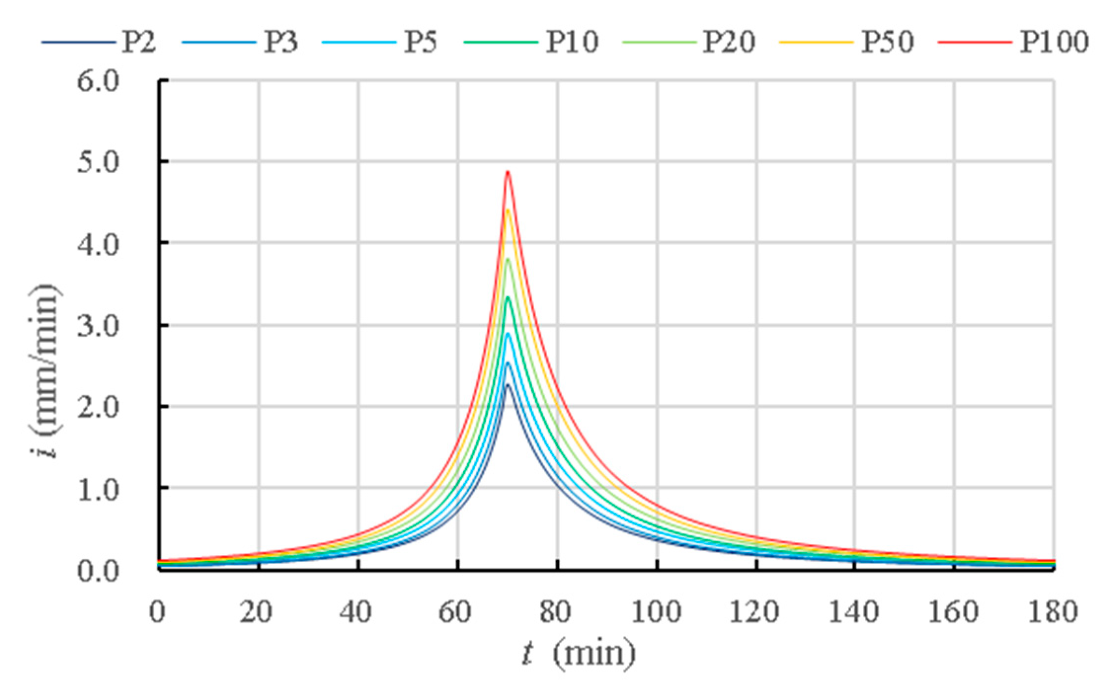
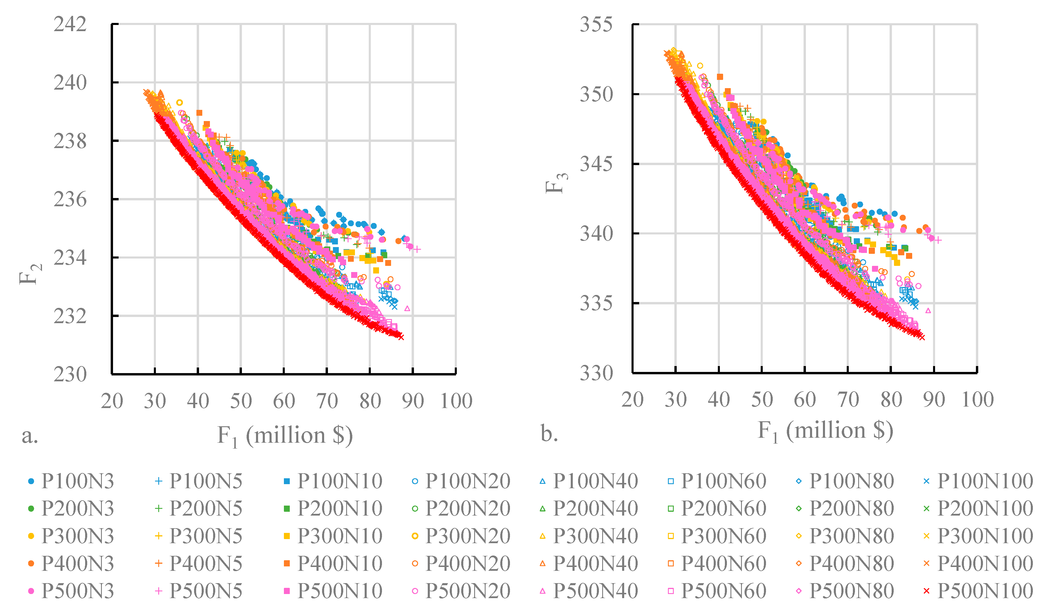
We obtain the optimal LID schemes using the SWMM-NSGA II. The optimal processes are conducted for a 180-min designed rainfall with return periods of 2 years. Several conditions of different generations (N) and populations (P) are considered in this study to find the impact on the Pareto front from the parameters of the NSGA II. With a small generation and population, the fronts composed by the solutions are far away from the Pareto front, and the width of the fronts are narrow (Figure 5). This means that NSGA II conducts a few search processes, and it is still difficult to approach the Pareto front with a small generation and population. As the population and generation increased, the fronts composed by the solutions are close to the Pareto front, and the width of the fronts become wide. It could be beneficial for the NSGA II to find the Pareto front with a bigger generation and population. However, this does not mean that a bigger generation and population are better and that the Pareto front could be found. If the generation was set at 100, the fronts of the solutions almost fell in the same line when the population increased from 300 to 500. This means that when the Pareto front was found, it could not improve the optimal with a bigger generation and population. In this study, we set the generation and population as 100 and 500, and the Pareto front is composed of all the 500 schemes (red × in Figure 5).

In Figure 5, when the $F_1$ increased, both the $F_2$ and $F_3$ decreased. It means that spending more money on the LIDs is benefit for reducing urban inundation and runoff pollution. We also found that the low cost of LID corresponds to the low effect of reducing runoff and pollutant concentration.

With the SDA, a suitable scheme could be selected from the Pareto set composed of 500 schemes. The entropy weights of the three objectives are 0.2979, 0.3544, and 0.3477. The weight of the $F_1$ is smaller than the weights of $F_2$ and $F_3$, which means that the entropy weights are beneficial for the objects $F_2$ and $F_3$. Then, scheme No. 94 is selected as the most suitable LID scheme because it has a minimum eigenvalue of 17.36. The $F_1$ is about 78 million CNY; the $F_2$ is 231.89, and the $F_3$ is 334.01. The area of CPP, VS, and RG are 14.18 ha, 4.81 ha, and 2.14 ha.

The SWMM model is responsible for describing the physical feature of an urban area. When the SWMM model of an urban area is settled, the physical features of the area are implied in the hydraulic and water quality outcomes. Then, these outcomes are provided to the NSGA II to select the optimal LID schemes based on the entropy weights calculated. Objectively, the entropy weights only show the importance of different optimization goals and are independent of scale and geographical features of the urban area.

The weight of the objectives in the SDA method could obviously affect the result. If we use the weights obtained using the entropy weight method, the scheme is selected objectively. However, people’s requirement might be the key factor in runoff and pollution management. We could change the weight to reflect the demand of the people in this method.

For example, the cost is a very important factor when deciding on the construction of urban infrastructures. When we try to reduce urban inundation or runoff pollution, the cost of LIDs is a vital constrain. A better reduction effectively results in a higher cost. But the fiscal revenue of an urban area is limited; this means that a manager should find the balance point between the reduction effective and cost. If we want to save more on the cost of the LIDs, we have to increase the weight of object $F_1$. For instance, we could change the weight of $F_1$ from 0.2979 to 0.90. To keep the sum of the weight equal to 1, the weights of $F_2$ and $F_3$ should be reduced. In this study, we thought that $F_2$ and $F_3$ were equally important, so their weights were set as 0.05 and 0.05. With the new weights, scheme No. 42 is selected as the most suitable LID scheme to save more cost, because it has a minimum eigenvalue of 13.82. The $F_1$ is about 31 million CNY; the $F_2$ is 238.68, and the $F_3$ is 350.44. The area of CPP, VS, and RG are 6.76 ha, 4.31 ha, and 0.91 ha. Scheme No. 42 could cost 47 million CNY less than scheme No. 94. It also shows that the weights could significantly affect the selection result.

In fact, there are lots of factors that might affect the construction of urban infrastructures, such as cost, policies, environmental protection, land ownership, etc. The method in this study focuses on three brief goals and could provide the decision makers with the LID scheme for reference. The decision makers could then develop more detailed LID plans based on the results given using this method.

4.2. Influence of the NSGA II Parameters

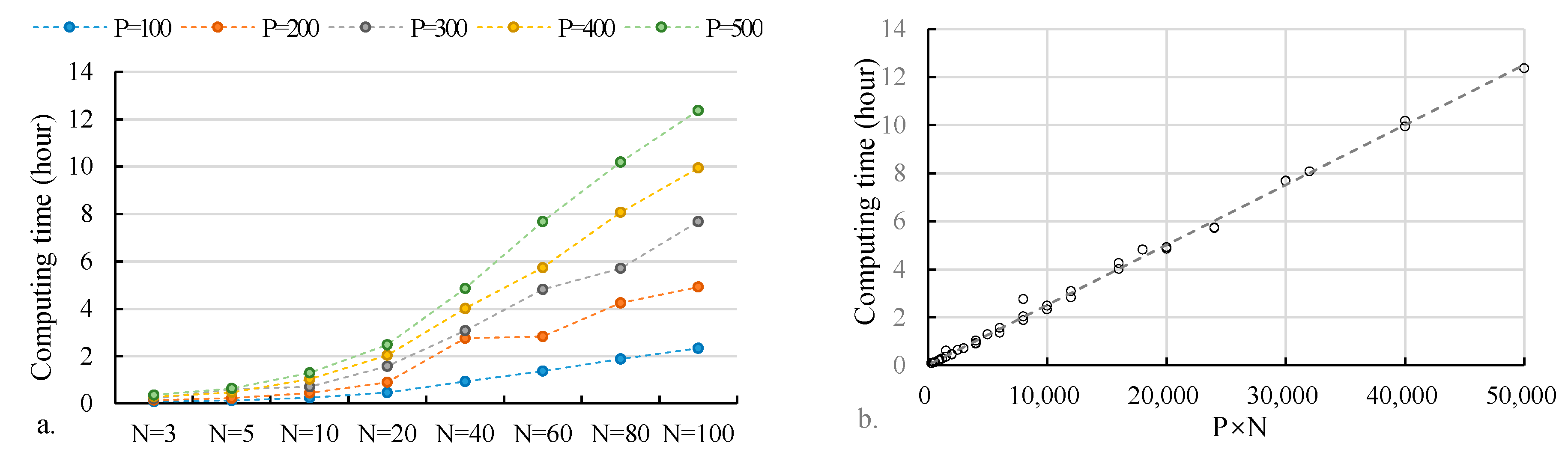
The generation (N) and population (P) are the important parameters of the NSGA II, and they would affect the effect of finding the proper LID schemes. We set up a numerical test to find the influence of these two parameters. We calculate the LID schemes with 40 combinations of different generations and populations.

Both the increase in generation and population of the NSGA II could obviously lead to an increase in computing time (Figure 6a). The computing time increases linearly with the product of P and N (Figure 6b).

The generation and population have a great influence on the Pareto fronts. When the generation increases, the results of the NSGA II approach better Pareto fronts (Figure 5). If the generation is the same, the Pareto fronts corresponding to different populations are almost gathered together in the middle, but the left and right sides of the Pareto fronts are slightly divergent. When the population increases, the curvatures of these Pareto fronts decrease, and the left and right sides of the Pareto fronts approach the front with the maximum population.

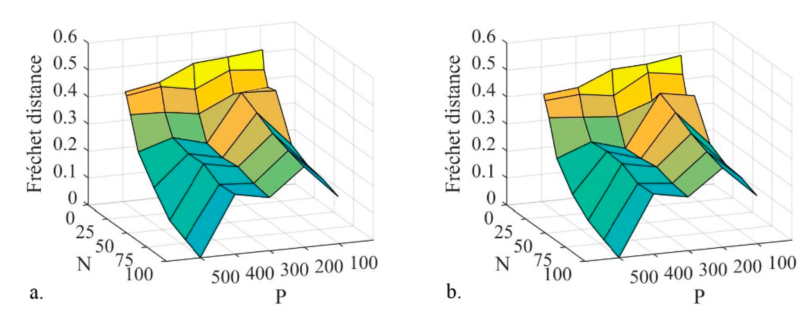
To evaluate the difference between different Pareto fronts with different combinations, we take the fronts as trajectories and use the Fréchet distance to evaluate the distance between the different trajectories [51]. The trajectory data can be discrete or continuous, and the number of points composing the two trajectories does not have to be the same [52]. We use the front (P = 500, N = 100) as the baseline. The other fronts are compared with the baseline front. The data of the fronts should be normalized before the Fréchet distance is calculated in order to eliminate dimensional differences. The Fréchet distance of different P and N are shown in Figure 7. Figure 7a shows the Fréchet distance of the fronts of $F_1$ and $F_2$, Figure 7b shows the Fréchet distance of the fronts of $F_1$ and $F_3$. The tendency of both figures are almost the same. When P ≥ 300 and N ≥ 100, the Fréchet distance is smaller than 0.2, and the fronts are close to the baseline fronts. This means we use a smaller P and N to find the approximate optimum schemes and save on computing time. In this study, P = 300 and N = 100 could be used to find the approximate optimum schemes, and this could save about 4 h of computing time.

4.3. Influence of the Rain Type

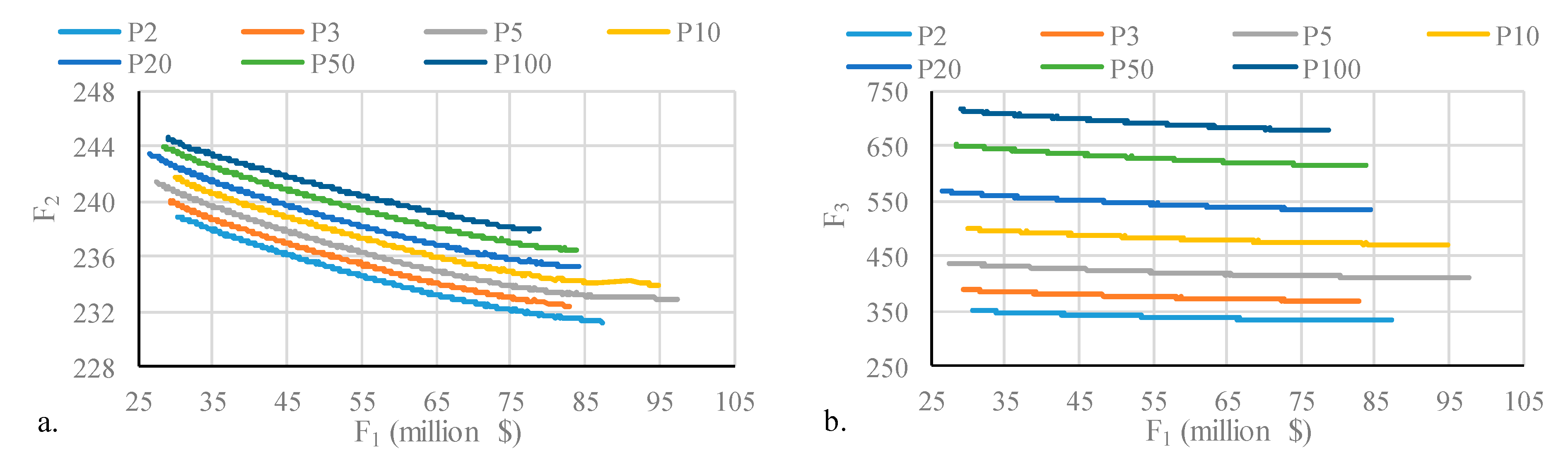
The return periods could affect the Pareto fronts. The optimal processes are conducted for a 180-min designed rainfall with return periods of 2 years, 3 years, 5 years, 10 years, 20 years, 50 years, and 100 years. With the same $F_1$, the increase in return period of rainfall resulted in the increase in $F_2$ and $F_3$. This has good agreement with the study conducted by Hai (2020) [48]. The increments of $F_2$ are smaller than the increments of $F_3$ with the variation in return periods in this study. When the rainfall increases, more pollutants are washed off by the runoff. This causes the obvious increment of $F_3$. Hai (2020) [48] found that the return period of the rainfall patterns which were utilized for the design of LID installment should not exceed 2 years. Figure 8 shows that if the return period increases from 2 years to 3 years, $F_3$ could not be reduced to the same level by just building more LIDs, which leads to cost increments. Cleaning the land surface might be the more efficient way to reduce the pollutants carried by the runoff.

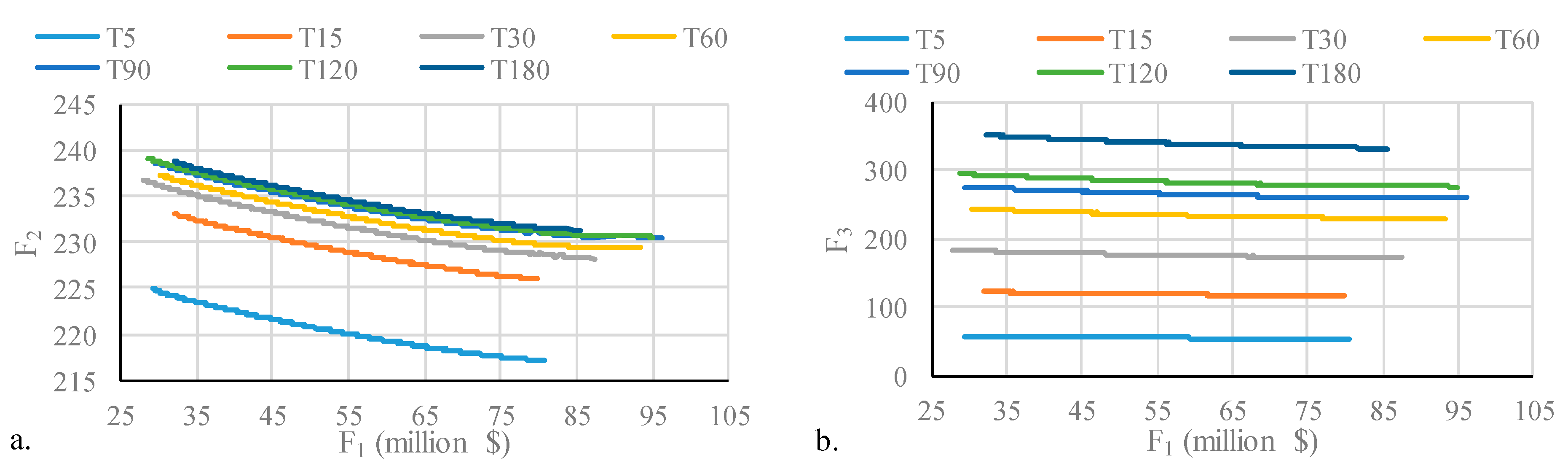
The rainfall duration also affects the cost-effectiveness curves. The optimal processes are conducted for a 2-year rainfall period with durations of 5 min, 15 min, 30 min, 60 min, 90 min, 120 min, and 180 min. The long duration causes more runoff which exceeds the capacity of the LIDs. As the runoff increases, the $r_i$ approaches 1, and the $F_2$ approaches the maximal value. Then, the Pareto fronts of long durations are close to each other. For this study case, if the duration exceeds 15 min, this means that the LIDs schemes could not handle the runoff, and the cost-effectiveness curves cluster together. The longer the duration, the bigger the $F_3$; this is because more pollutants are washed off by the increased runoff. Figure 9 shows that $F_2$ and $F_3$ could not be reduced to the same level by just building more LIDs which leads to cost increments when the duration increases a lot. It also shows that the LIDs could be ineffective for less frequent, heavier, and longer duration storms, and the LIDs might be taken as assistance measures for conventional runoff management practices and drainage systems [11,16].

4.4. Cost and LIDs for Different Objectives

For different objectives, the costs of LIDs are different. If we want to control more runoff or pollution, the cost might be increased (

Table 8. Area and cost of LIDs of F₁_Min and F₃_Max as well as F₁_Max and F₃_Min.

Cases	LID	5 min	15 min	30 min	60 min	90 min	120 min	180 min	Average
F1_Min and F3_Max	CPP	54.26%	56.21%	54.58%	55.26%	56.33%	52.94%	56.46%	55.15%
	VS	38.11%	36.23%	35.66%	36.05%	35.48%	37.94%	35.95%	36.49%
	RG	7.63%	7.56%	9.76%	8.68%	8.19%	9.12%	7.58%	8.36%
LID Area (ha)		11.11	11.99	10.09	11.22	11.72	10.52	11.98	11.07
Cost (million CNY)		29.38	32.14	27.96	30.33	29.38	28.79	32.26	30.04
F1_Max and F3_Min	CPP	67.00%	69.71%	66.35%	73.20%	73.14%	70.35%	69.41%	69.88%
	VS	20.62%	17.84%	21.31%	15.30%	14.50%	17.48%	17.68%	17.82%
	RG	12.37%	12.45%	12.35%	11.50%	12.36%	12.17%	12.91%	12.30%
LID Area (ha)		138.22	134.03	150.80	155.01	157.51	159.14	142.17	148.13
Cost (million CNY)		80.61	79.96	87.44	93.23	96.25	94.82	85.49	88.26

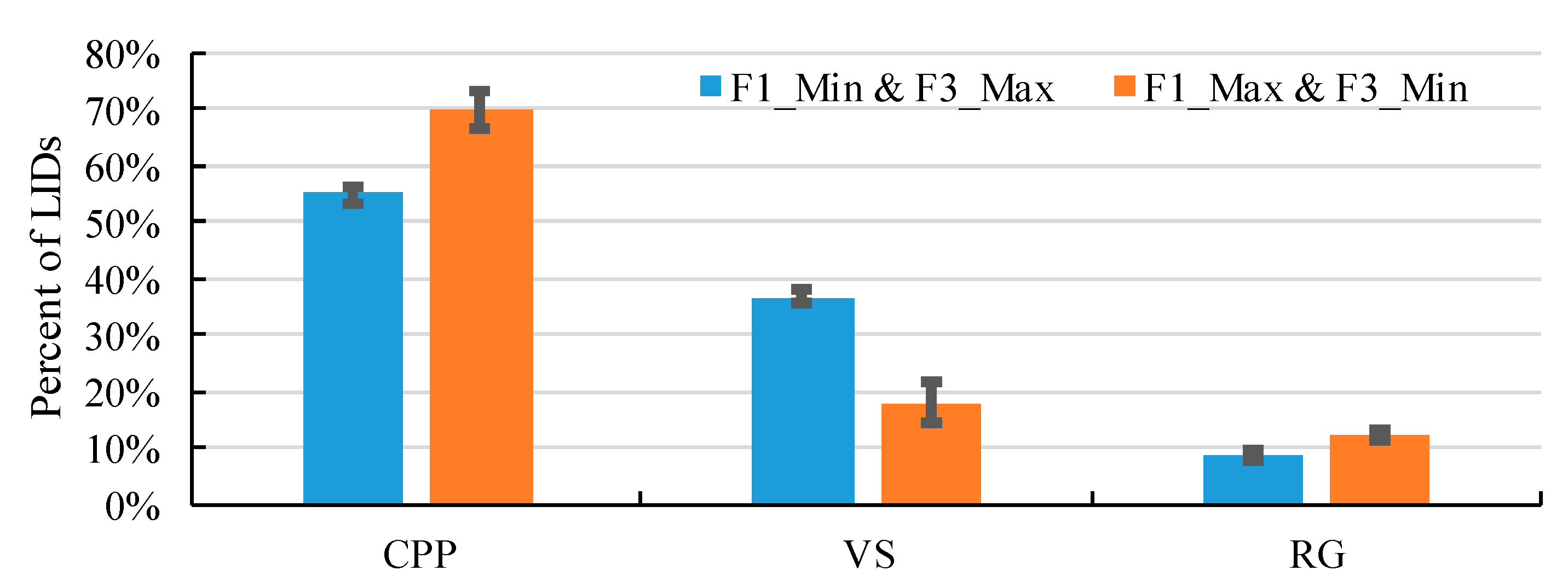
, Figure 8 and Figure 9). We took the LID schemes for 2 years of rainfall as an example. We set two cases, the first is that the $F_1$ reaches the minimum, and the $F_3$ reaches the maximum; the second is that the $F_1$ reaches the maximum, and the $F_3$ reaches the minimum.

If the $F_1$ reaches the minimum and the $F_3$ reaches the maximum, the CPP average area percent is about 55% of the land which could be used to construct LIDs, and the percentages of the VS and rain garden are about 37% and 8% (Table 5 and Figure 10). When the $F_1$ reaches the maximum and the $F_3$ reaches the minimum, the percent of CPP area is about 70%, and the percentages of the VS and RG are about 17% and 13% (Table 5 and Figure 10). To minimize $F_3$, both CPP and the RG are increased, and the VS is reduced, as the CPP and the RG could handle more runoff and reduce more pollutants. The error bars in Figure 10 show the percentages of these LID change slightly when the rainfall duration increases from 5 min to 180 min. Though this change is slight, it could obviously cause the LID cost to increase. For the minimum $F_1$, when the rainfall duration increases from 5 min to 180 min, the percentage of LID area changes within 2.2%. However, the left endpoints of the cost-effective curves vary from 28 million CNY to 33 million CNY (Figure 9); this means that the LID cost could vary within 5 million CNY. For the minimum $F_3$, when the percent of LID area changes within 4%, the right endpoints of the cost-effective curves vary from 81 million CNY to 96 million CNY; this means that the LID cost could vary within 15 million CNY.

4.5. Space Distribution of the LIDs

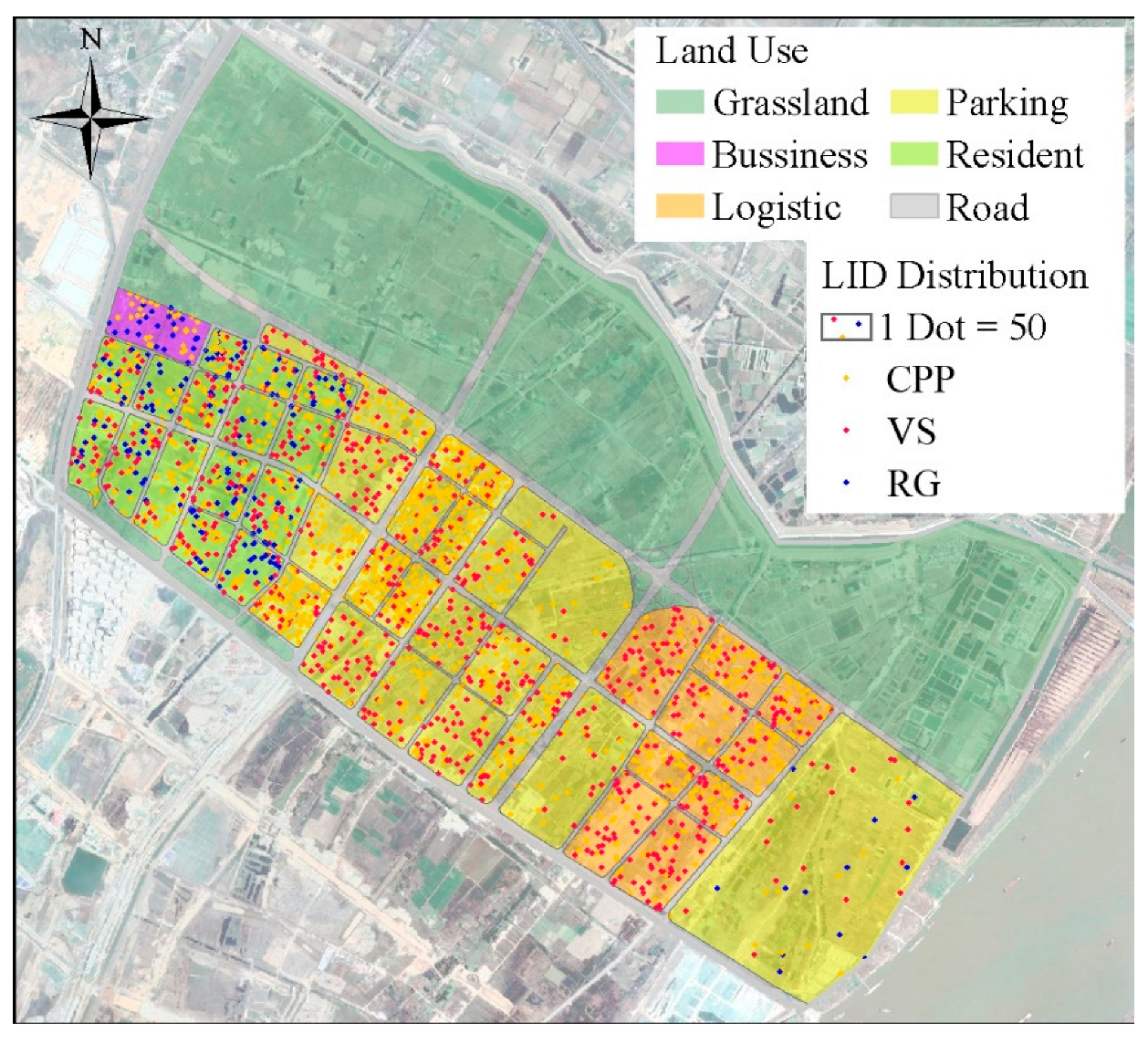
We could find the space distribution of the LIDs corresponding to the scheme which was figured out using the method used in this paper. The type and quantity of the LIDs in each subcatchment of the SWMM model could be counted. For example, a dot density map could be used to show the spatial distribution of the LIDs for a 2-year rainfall period with a duration of 180 min. Each dot represents a LID area of 50 m². Figure 11 shows the spatial distribution of LID for the maximum $F_1$ and minimum $F_3$. 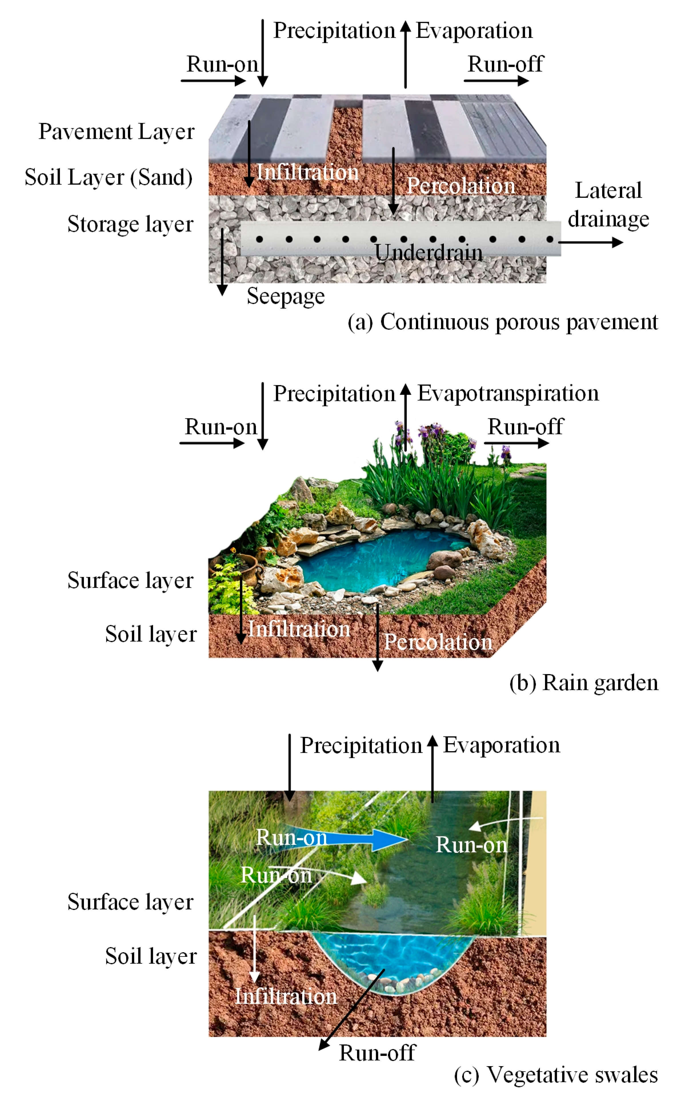The rain garden (bioretention) is highly efficient and is beneficial for the sightseeing of both residential and commercial settings [41], so most of the RGs are distributed in the resident and business areas which are covered by buildings with an impervious area. The CPP and VS are used in the logistic and parking areas where the beautiful scenery is not the major demand.

The optimization results should be interpreted in the context of a specific problem, namely optimization goals unique to this case study. If the optimization targets or the area constrains of each LID type were changed, the spatial distribution might change too.

5. Conclusions

This paper focuses on choosing the proper optimal LID planning alternative for an intending urban area. First, we employed the SWMM and NSGA II to compose an integrated model to find the optimal LID planning alternatives. Then, the structural decision-making approach for a multi-objective system is used to find the proper optimal LID plan from the multi-objective optimization results. We conclude this work as follows:

• The SWMM-NSGA II model could be used to find the multi-objective optimization LID plans for an intending urban area. With its help, we found the proper LID plan for the study area from 500 schemes which consisted of the Pareto set. The scheme costing 78 million CNY was selected when the entropy weights were used in the SDA method. If we considered saving more cost, the scheme costing 31 million CNY was selected with the artificially modified weights;
• The aim runoff coefficient and aim pollutant concentration of the SWMM-NSGA II model could be set for each subcatchment, and the types and amount of LID used in each subcatchment could be given by the model due to the control aim of each subcatchment. Because the aim of this method could be set flexibly and the SWMM is a physically based model, the method could be applied to other urban areas where the LIDs are going to be constructed.;
• The computing time increases linearly with the product of the generation and population in NSGA II. Though a large generation and population could be beneficial for approaching the Pareto fronts, we use the second largest generation and population to approach the Pareto fronts while saving computing time;
• The structural decision-making approach for a multi-objective system (SDA) could be used to select for a suitable scheme from the Pareto set composed of optimal alternatives. Because the weight of the objectives in the SDA method could affect the result, the selection process could be turned into an interactive process. Firstly, the entropy weight method could be used to objectively select the scheme. Then, the entropy weights could be taken as a referable option and changed artificially to reflect the management demand of people;
• The LIDs are quite essential to control the quantity and quality of urban storm water runoff for frequent, lighter, and shorter duration storms. The higher costs might not correspond to an obvious control effective in a heavy storm. The control effective for more frequent, lighter, and shorter duration storms is more important when deciding the LID plan;
• Though the SWMM-NSGA II model could find the optimal LID schemes, it is very time-consuming. The high-performance computing method or meta-model with artificial intelligence (AI) technology might be employed to provide more efficient methods to find the Pareto fronts. AI combined with expert knowledge could be more helpful for making the decision of constructing urban infrastructures in the future.

References

1. Hsieh, C.; Davis, A.P. Evaluation and optimization of bioretention media for treatment of urban storm water runoff. J. Environ. Eng. 2005, 131, 1521–1531. [Google Scholar] [CrossRef]
2. United States Environmental Protection Agency. Low Impact Development (LID) A Literature Review; EPA: Washington, DC, USA, 2000; pp. 1–9.
3. Himanshu, S.K.; Pandey, A.; Yadav, B.; Gupta, A. Evaluation of best management practices for sediment and nutrient loss control using SWAT model. Soil Till. Res. 2019, 192, 42–58. [Google Scholar] [CrossRef]
4. Johnson, D.; Geisendorf, S. Are Neighborhood-level SUDS Worth it? An Assessment of the Economic Value of Sustainable Urban Drainage System Scenarios Using Cost-Benefit Analyses. Ecol. Econ. 2019, 158, 194–205. [Google Scholar] [CrossRef]
5. Meng, T.; Hsu, D. Stated preferences for smart green infrastructure in stormwater management. Landsc. Urban Plan. 2019, 187, 1–10. [Google Scholar] [CrossRef]
6. Ashkok, K.S.; Ted, G.; Don, B. Approaches to Water Sensitive Urban Design; Elsevier: Amsterdam, The Netherlands, 2019; pp. 1–24. [Google Scholar]
7. Ding, N.; Hu, A.B.; Ren, X.X. Application and prospect of low impact development model in Shenzhen. Water Wastewater Eng. 2012, 38, 141–144. [Google Scholar]
8. Long, Y.Q.; Gai, Y.W.; Guan, X.K.; Hu, X.Y.; Cui, T.T. Advance of the Method estimating the Benefit of Storm Water Usage in Urban Area. In Proceedings of the 2018 International Conference of Green Buildings and Environmental Management, Qingdao, China, 23–25 August 2018. [Google Scholar]
9. General Office of the State Council of the People’s Republic of China. Guidance on Promoting the Construction of the Sponge City; General Office of the State Council of the People’s Republic of China: Beijing, China, 2015.
10. Guo, W.X.; Liu, W.Y.; Wang, H.X. Study and Application of Ecological Management of Urban Rain and Flood Resources; China Water Power Press: Beijing, China, 2015; pp. 7–16. [Google Scholar]
11. Cui, T.T.; Long, Y.Q.; Wang, Y.T. Choosing the LID for Urban Storm Management in the South of Taiyuan Basin by Comparing the Storm Water Reduction Efficiency. Water 2019, 11, 2583. [Google Scholar] [CrossRef]
12. Freni, G.; Mannina, G.; Viviani, G. Urban storm-water quality management: Centralized versus source control. J. Water Resour. Plan. Manag. 2010, 136, 268–278. [Google Scholar] [CrossRef]
13. Eckartx, K.; Mcpheex, Z.; Bolisetti, T. Performance and implementation of low impact development—A review. Sci. Total Environ. 2017, 607, 413–432. [Google Scholar] [CrossRef] [PubMed]
14. Ehsan, R.; Alizadeh, M.R.; Nikoo, M.R.; Adamowski, J. Multi-objective decision-making for green infrastructure planning (LID-BMPs) in urban storm water management under uncertainty. J. Hydrol. 2019, 579, 124091. [Google Scholar]
15. Bosley, E.K. Hydrologic Evaluation of Low Impact Development Using a Continuous, Spatially-Distributed Model. Master’s Thesis, Virginia Polytechnic Institute and State University, Blacksburg, VA, USA, 2008. [Google Scholar]
16. Mo, W.; Zhang, D.Q.; Lou, S.W.; Hou, Q.H.; Liu, Y.J.; Cheng, Y.; Qi, J.D.; Tan, S.K. Assessing Hydrological Effects of Bioretention Cells for Urban Stormwater Runoff in Response to Climatic Changes. Water 2019, 11, 997. [Google Scholar] [CrossRef]
17. Silva, T.; Vinon-leite, B.; Lemaire, B.J.; Petrucci, G.; Nascimento, O. Impact of Urban Stormwater Runoff on Cyanobacteria Dynamics in A Tropical Urban Lake. Water 2019, 11, 946. [Google Scholar] [CrossRef]
18. Rezaei, A.R.; Lsmail, Z.; Niksokhan, M.H.; Dayarian, M.A.; Shirazi, S.M. A Quantity–Quality Model to Assess the Effects of Source Control Stormwater Management on Hydrology and Water Quality at the Catchment Scale. Water 2019, 11, 1415. [Google Scholar] [CrossRef]
19. Jia, H.; Yao, H.; Shaw, L.Y.; Lu, Y. Development of a multi-criteria index ranking system for urban runoff best management practices (BMPs) selection. Environ. Monit. Assess. 2013, 189, 7915–7933. [Google Scholar] [CrossRef]
20. Chiang, L.C.; Chaubey, I.; Maringanti, C.; Huang, T. Comparing the selection and placement of best management practices in improving water quality using a multi-objective optimization and targeting method. Int. J. Environ. Res. Public Health 2014, 11, 2992–3014. [Google Scholar] [CrossRef]
21. Ghodsi, S.H.; Kerachian, R.; Malakpour Estalaki, S.; Nikoo, M.R.; Zahmatkesh, Z. Developing a stochastic conflict resolution model for urban runoff quality management: Application of info-gap and bargaining theories. J. Hydrol. 2016, 533, 200–212. [Google Scholar] [CrossRef]
22. Zhang, K.; Chui, T.M. A comprehensive review of spatial allocation of LID-BMP-GI practices: Strategies and optimization tools. Sci. Total Environ. 2018, 621, 915–929. [Google Scholar] [CrossRef]
23. Sebti, A.; Carvallo Aceves, M.; Bennis, S.; Fuamba, M. Improving nonlinear optimization algorithms for BMP implementation in a combined sewer system. J. Water Resour. Plann. Manag. 2016, 142, 04016030. [Google Scholar] [CrossRef]
24. Song, J.Y.; Chung, E. A multi-criteria decision analysis system for prioritizing sites and types of low impact development practices: Case of Korea. Water 2017, 9, 291. [Google Scholar] [CrossRef]
25. Duan, H.-F.; Li, F.; Yan, H. Multi-objective optimal design of detention tanks in the urban stormwater drainage system: LID implementation and analysis. Water Resour. Manag. 2016, 30, 4635–4648. [Google Scholar] [CrossRef]
26. Huang, C.L.; Hsu, N.S.; Liu, H.J.; Huang, Y.H. Optimization of low impact development layout designs for megacity flood mitigation. J. Hydrol. 2018, 564, 542–558. [Google Scholar] [CrossRef]
27. Deb, K.; Pratap, A.; Agrawal, S.; Meyarivan, T. A fast and elitist multi-objective genetic algorithm: NSGA-II. IEEE Trans. Evol. Comput. 2002, 6, 182–197. [Google Scholar] [CrossRef]
28. Niksokhan, M.H.; Kerachian, R.; Karamouz, M. A game theoretic approach for trading discharge permits in rivers. Water Sci. Technol. 2009, 60, 793–804. [Google Scholar] [CrossRef] [PubMed]
29. Zare, S.O.; Saghafian, B.; Shamsai, A. Multi-objective optimization for combined quality–quantity urban runoff control. Hydrol. Earth Syst. Sci. 2012, 16, 4531–4542. [Google Scholar] [CrossRef]
30. Macro, K.; Matott, L.S.; Rabideau, A.; Seyed, H.G.; Zhu, Z.D. OSTRICH-SWMM: A new multi-objective optimization tool for green infrastructure planning with SWMM. Environ. Modell. Softw. 2019, 113, 42–47. [Google Scholar] [CrossRef]
31. Chen, S. Fuzzy Recognition Theory and Application for Optimizing Complex Water Resources Systems; Jilin University Press: Changchun, China, 2008; pp. 73–82. [Google Scholar]
32. Zhang, S.; Guo, Y. SWMM simulation of the storm water volume control performance of permeable pavement systems. J. Hydrol. Eng. 2014, 20, 06014010. [Google Scholar] [CrossRef]
33. Rossman, L.A.; Wayne, C.H. SWMM Reference Manual Volume III—Water Quality; National Risk Management Laboratory: Cincinnati, OH, USA, 2016; pp. 99–118. [Google Scholar]
34. Rossman, L.A. SWMM Reference Manual Volume II—Hydraulics; National Risk Management Laboratory: Cincinnati, OH, USA, 2017; pp. 31–38. [Google Scholar]
35. Horton, R.E. An approach toward a physical interpretation of infiltration capacity. Soil Sci. Soc. Am. J. 1940, 5, 399–417. [Google Scholar] [CrossRef]
36. Bai, Y.R.; Na, Z.; Zhang, R.Y.; Zeng, X.F. Storm Water Management of Low Impact Development in Urban Areas Based on SWMM. Water 2019, 11, 33. [Google Scholar] [CrossRef]
37. Ammon, D.C. Urban Stormwater Pollutant Buildup and Washoff Relationships. Master’s Thesis, University of Florida, Gainesville, FL, USA, 1979. [Google Scholar]
38. US Environmental Protection Agency. Results of the Nationwide Urban Runoff Program (NURP); NTIS PB 84-185552; U.S. Environmental Protection Agency: Washington, DC, USA, 1983.
39. Ma, Y. Research on Transportation Simulation of Urban Rainfall-Runoff Non-Point Source Pollution and the First Flush Effects. Master’s Thesis, South China University of Technology, Guangzhou, China, 2012. [Google Scholar]
40. Huang, T. Practical Study on Urban Rainfall Runoff LID-BMPs. Master’s Thesis, Suzhou University of Science and Technology, Suzhou, China, 2014. [Google Scholar]
41. Dietz, M.E. Low impact development practices: A review of current research and recommendations for future directions. Water Air Soil Pollut. 2007, 186, 351–363. [Google Scholar] [CrossRef]
42. Ismail, A.F.; Sapari, N.; Wahab, M.A. Vegetative swale for treatment of stormwater runoff from construction site. Pertanika J. Sci. Technol. 2014, 22, 55–64. [Google Scholar]
43. LID Controls. Available online: https://support.chiwater.com/77701/lid-controls (accessed on 16 June 2019).
44. William, M. Landscape Planning: Environmental Application, 5th ed.; John Wiley & Sons, Inc.: Hoboken, NJ, USA, 2010; pp. 147–164. [Google Scholar]
45. Ren, X.; Yu, L.; Hu, A.; Zhang, L.; Li, C. Planning and Management of Sponge City Construction; China Architecture Publishing & Media Co., Ltd.: Beijing, China, 2017; pp. 218–221. [Google Scholar]
46. Seinivas, N.; Deb, K. Multi-objective optimization using nondominated sorting genetic algorithms. Evol. Comput. 1995, 2, 221–248. [Google Scholar] [CrossRef]
47. Wu, J.; Kauhanen, P.G.; Hunt, J.A.; Senn, D.B.; Mckee, L.J. Optimal Selection and Placement of Green Infrastructure in Urban Watersheds for PCB Control. J. Sustain. Water. Buil. 2019, 5, 04018019. [Google Scholar] [CrossRef]
48. Hai, D.M. Optimal Planning of Low-Impact Development for TSS Control in the Upper Area of the Cau Bay River Basin, Vietnam. Water 2020, 12, 533. [Google Scholar] [CrossRef]
49. Jiang, J. Study and Application of Theory and Evaluation Architecture of Groundwater Environment Health. Ph.D. Thesis, Jilin University, Changchun, China, 2007. [Google Scholar]
50. Rainstorm Intensity Formula (Revised) of Nanjing. Available online: https://max.book118.com/html/2017/0921/134625168.shtm (accessed on 29 April 2021).
51. Alt, H.; Godau, M. Computing the Fréchet distance between two polygonal curves. Int. J. Comput. Geom. Appl. 1995, 5, 75–91. [Google Scholar] [CrossRef]
52. MATLAB Central File Exchange. Available online: https://www.mathworks.com/matlabcentral/fileexchange/41956-frechet-distance-calculator (accessed on 29 April 2021).
Figure 1. The location of the study area. (a) The location of the study site; (b) The SWMM model of the study site.
Water 17 00154 g001
Figure 2. The process of deciding the LID scheme.
Water 17 00154 g002
Figure 3. Continuous porous pavement, rain garden, and vegetative swales. (a) The structure of the continuous pavement; (b) The structure of the rain garden; (c) The structure of vegetative swales.
Water 17 00154 g003
Figure 4. The rainfall in Nanjing.
Water 17 00154 g004
Figure 5. The Pareto fronts of the LID schemes. (a) The Pareto fronts of objectives F1 and F2 corresponding to different population and generation; (b) The Pareto fronts of objectives F1 and F3 corresponding to different population and generation. The P and N represent the population and generation of the NSGA II, respectively. The number behind P and N are their corresponding values. The points of the same generation have the same shape. The points of the same population have the same color. When the population increases, the color of the points changes from light blue to dark pink. The Pareto fronts composed of all the 500 schemes are represented with red ×.
Water 17 00154 g005
Figure 6. The relationship between the computing time, generation, and population. (a) The computing time of different P and N; (b) The computing time of different P × N.
Water 17 00154 g006
Figure 7. The Fréchet distance of different P and N. (a) The P Fréchet distance of the fronts of F 1 and F 2 ; (b) The Fréchet distance of the fronts of F 1 and F 3 .
Water 17 00154 g007
Figure 8. The influence of the return periods to Pareto fronts. (a) The Pareto fronts of objectives F1 and F2 corresponding to different return periods; (b) The Pareto fronts of objectives F1 and F3 corresponding to different return periods. P represents the return period of the rainfall. The number behind P is the value of the return period.
Water 17 00154 g008
Figure 9. The influence of the rainfall duration to Pareto fronts. (a) The Pareto fronts of objectives F1 and F2 corresponding to different rainfall durations; (b) The Pareto fronts of objectives F1 and F3 corresponding to different rainfall durations. T represents the rainfall durations. The number behind T is the value of the rainfall durations.
Water 17 00154 g009
Figure 10. The percent of LID utilization.
Water 17 00154 g010
Figure 11. The spatial distribution of LID utilization for a 2-year rainfall period with a duration of 180 min.
Water 17 00154 g011