Article

Shallow Hydrostratigraphy Beneath Marsh Platforms: Insights from Electrical Resistivity Tomography

by
Jacque L. Kelly
* and
Christine M. Hladik
School of Earth, Environment and Sustainability, Georgia Southern University, Statesboro, GA 30458, USA
*
Author to whom correspondence should be addressed.
Water 2025, 17(2), 144; https://doi.org/10.3390/w17020144
Submission received: 14 November 2024 / Revised: 31 December 2024 / Accepted: 4 January 2025 / Published: 8 January 2025

Abstract

:
Salt marshes are ecologically and economically valuable ecosystems, yet are vulnerable to marsh dieback, the rapid death of marsh vegetation, which has affected coastal areas along the southeastern and Gulf coasts of the United States in recent decades. This study used multichannel electrical resistivity tomography (ERT) surveys to investigate the shallow hydrostratigraphy (up to 39.2 m depth) of three dieback-affected salt marshes along the Georgia coast to evaluate the influence of site location, vegetation status (dieback versus healthy), and tidal conditions on ERT profiles. ERT profiles revealed consistent subsurface resistivity patterns across the marsh platforms, with low resistivity (0.2 ohm-m) at shallow depths indicating saltwater saturation and a transition to higher resistivity (up to 8.1 ohm-m) at greater depths, potentially signifying a shift to brackish conditions and/or sandy strata. The ERT data indicated that the hydrostratigraphy is similar across all study sites. Furthermore, the ERT data remained consistent regardless of vegetation status, tidal variations, and seasonal changes, suggesting that the processes driving the recovery of marsh dieback are independent of the shallow marsh stratigraphy. These findings enhance our understanding of marsh subsurface conditions, supporting efforts to better understand marsh resilience and guide future research on salt marshes.

1. Introduction

Salt marshes are valuable ecological and economic systems. They provide critical breeding and foraging habitats for a diverse array of aquatic and terrestrial organisms. They also improve water quality through nutrient and metal removal, sequester carbon, and provide crucial protection to developed coastal areas from shoreline erosion and storms [1,2]. Despite their ecological significance, salt marshes are vulnerable ecosystems that have experienced marsh dieback throughout the United States (US) Atlantic and Gulf Coasts [3,4,5,6,7], including coastal Georgia, since at least 2001 [4,8]. Marsh dieback is characterized by a rapid senescence of salt marsh vegetation. It particularly impacts Spartina alterniflora (marsh cordgrass) and Juncus roemerianus (black needlerush). This phenomenon has been extensively documented, affecting over 8 km2 in coastal Georgia [8,9]. Marsh dieback leads to the complete loss of vegetation structures, resulting in large mudflats that are vulnerable to erosion and loss of elevation, which further hinders marsh recovery [3,10,11,12]. Observations have shown dieback across various elevations, from low-lying creek banks to higher-elevation upland borders [9].
The causes of marsh dieback in coastal Georgia have been attributed to abiotic and biotic variables, including soil biogeochemistry, fungal pathogens, and consumer food webs [8]. While a single definitive cause is rarely identified, a multi-stressor hypothesis associated with drought conditions is most widely accepted for dieback in Georgia [8]. Groundwater dynamics influence salt marsh ecosystems, impacting soil salinity, nutrient cycling, marsh productivity, and plant species distribution [4,13,14]. In marshes, dissolved oxygen in shallow groundwater is impacted by vegetation roots, which typically grow 12 to 20 cm deep for S. alterniflora [15] and 30 to 60 cm deep for J. roemerianus [16]. This interaction also contributes nutrients to the ecosystem [17]. Despite its importance, the subsurface environment of salt marshes remains underexplored. In particular, little is known about how the shallow marsh hydrostratigraphy interacts with marsh dieback and recovery processes. Previous studies have primarily focused on surface conditions, overlooking the potential influence of subsurface hydrology. During droughts, for instance, shallow aquifers become highly susceptible to salinization due to reduced recharge from local precipitation [4]. Additionally, drought conditions can dry the marsh surface and increase porewater salinity when evapotranspiration proceeds in the absence of precipitation [4]. Moreover, coastal aquifers provide hydrologic connections between marshes and estuaries [17]. The aquifers influence estuarine water chemistry, which increases dynamic mixing in the reaction zones, where the water chemistry changes drastically with tidal fluctuations [17]. Given the association between drought, changes in groundwater dynamics, and marsh dieback, a more comprehensive investigation of groundwater below the salt marsh platform is needed. This study, therefore, aims to examine the shallow hydrostratigraphy of salt marsh platforms and their relationship to marsh dieback and recovery.
Multichannel electrical resistivity tomography (ERT) is a powerful geophysical tool for noninvasive exploration of shallow subsurface environments [18]. ERT surveys deliver detailed subsurface images, making them highly effective in detecting clay-dominated strata and differentiating between freshwater- and saltwater-saturated sediments [18]. Such surveys have characterized subsurface geology and hydrogeology, revealed stratigraphic heterogeneities, and defined freshwater-seawater boundaries in coastal aquifers [18,19,20]. This technique works well in coastal environments because freshwater and seawater differ in their electrical resistivity properties [18,19]. Additionally, ERT surveys provide insights into the geometry of the groundwater seepage conduits and the movement and mixing of groundwater and seawater in coastal aquifers [18,19]. Resistivity profiles are a function of the underlying lithology, porosity, water salinity, and temperature [20] and, therefore, reflect bulk resistivity (resistivity is the inverse of conductivity) of the subsurface materials. ERT’s capability to measure bulk resistivity makes it a valuable tool for examining the hydrostratigraphy of aquifers and aquitards in coastal environments. In this study, we present the shallow hydrostratigraphy (<40 m) as revealed by ERT surveys from three salt marshes located along a latitudinal gradient of the Georgia coast, US. This study uses bulk resistivity to identify subsurface resistivity patterns beneath salt marshes and evaluates whether the resistivity patterns vary based on site location, marsh vegetation type, marsh vegetation health and zonation, seasonal dynamics, and tidal flooding. Our results, therefore, offer insights into the geological and hydrological characteristics of these vulnerable salt marsh ecosystems.

2. Materials and Methods
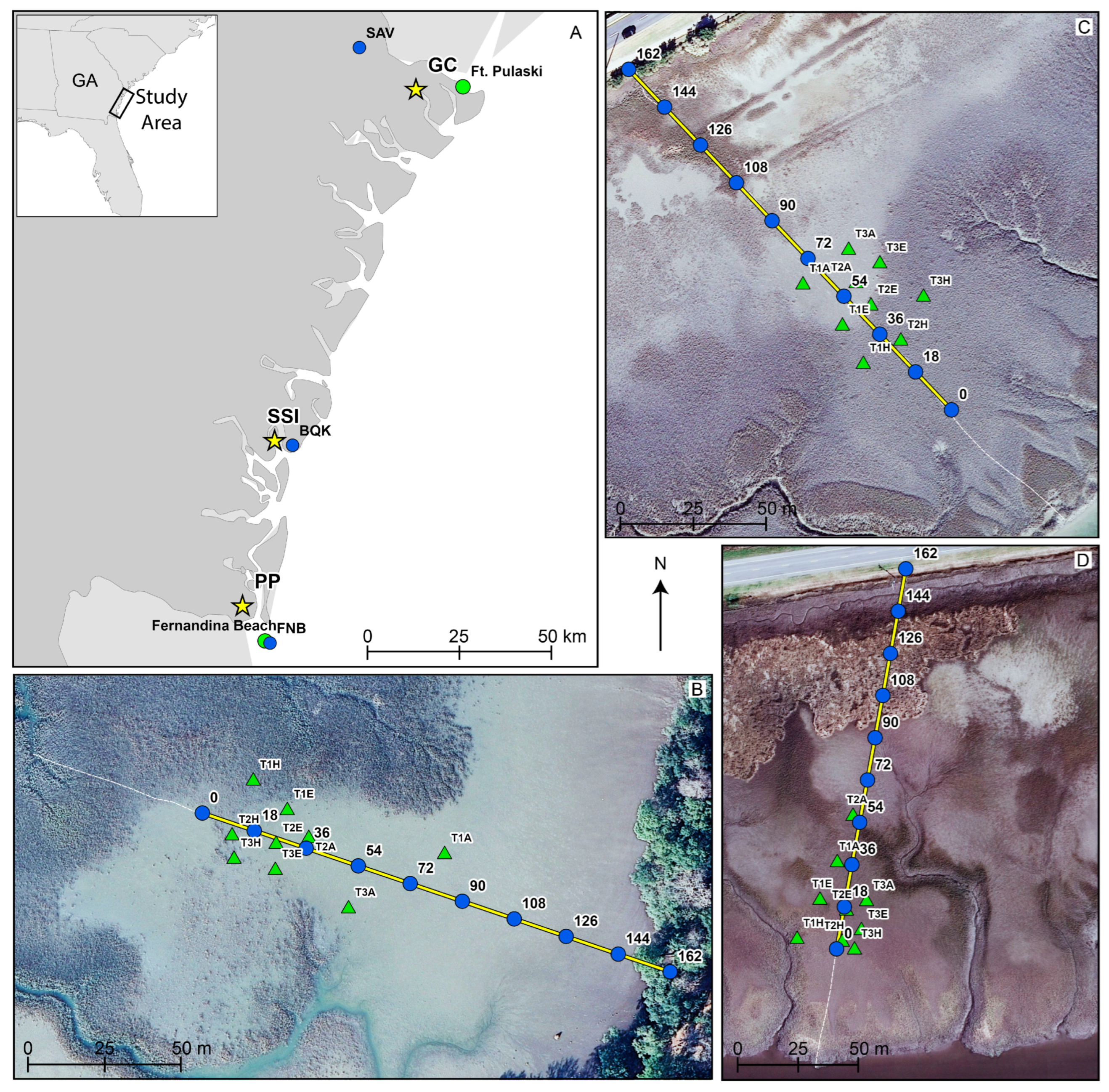
2.1. Study Sites

The Georgia coast is characterized by a subtropical climate with long, hot summers and short, mild winters [21] and spans a 160 km section of southeastern North America along the Western North Atlantic. The region’s lower coastal plain gives way to an extensive network of coastal wetlands, salt marshes, river deltas, and meandering tidal rivers, leading to an outer chain of barrier islands facing the Atlantic Ocean [22]. Within this setting, we collected field data at three marsh dieback locations (Figure 1A) that were dominated by the foundation species S. alterniflora. Dieback at our field sites was restricted to the interior marsh at distances exceeding 75 m from the tidal creeks, consistent with findings from Schepers et al. [7]. In the subtropical climate, S. alterniflora production is responsive to abiotic drivers year-round. Thus, we sampled quarterly (October–November, March, and July) from November 2014 to July 2016.
Site names were assigned based on location (Figure 1A), and abbreviations are as follows from north to south: Gray’s Creek (GC), St. Simons Island (SSI), and Point Peter (PP). For geospatial analyses presented below, all data used a common horizontal (North American Datum (NAD) 83(2011)/Universal Transverse Mercator (UTM) Zone 17N, European Petroleum Survey Group (EPSG): 6346) and North American Vertical Datum (NAVD) 88, GEOID 12A, EPSG: 5703) in unit meters. The GC site is located at 496,468.97mE 3,543,772.09mN (32.030289° N, 81.037223° W) near the city of Savannah. It is bounded by an urban housing development on the east and a tidal river called Grays Creek on the west (Figure 1B). S. alterniflora is the dominant vegetation at this site. The SSI site is located at 457,978.70mE 3,448,034.98mN (31.165996° N, 81.441708° W) off the F.J. Torras Causeway between St. Simons Island and the city of Brunswick (Figure 1C). This site is bordered by the F.J. Torras Causeway on the north–northwest and the tidal Mackay River on the south–southeast. Data from SSI were collected exclusively from S. alterniflora-dominated areas, avoiding areas with salt pans. Borrichia frutescens (sea ox-eye) and J. roemerianus are found along the upland border of the SSI site. The PP site is located at 449,154.00mE 3,403,002.81mN (30.759840° N, 81.531281° W) near the city of St. Marys and is bounded by the North River Causeway to the north and the tidal St. Marys River to the south (Figure 1D). In addition to S. alterniflora, J. roemerianus is present at this site near the causeway (Figure 1D), and both species are included in the ERT data at this site.
We established three shore-perpendicular transects (212 to 221 m in length; Table 1) at each site. The transects (T1, T2, and T3) were spaced ~15 m lateral distance from each other and extended from the upland border to the creek bank. Each transect bisected healthy (H), transitional edge (E), and affected dieback (A) condition classes of the marsh. For clarity, only T2 is shown as yellow lines in Figure 1B–D, as this is the transect from which the ERT data were collected. A permanent monitoring plot was established for each condition class (e.g., GC T1A, GC T1E, GC T1H) along each transect at each field site (green triangles in Figure 1B–D). Field data consisted of (1) real-time kinematic (RTK) Global Positioning System (GPS) measurements of elevation along each transect for all sampling dates, (2) standard water quality measurements (temperature, salinity, specific conductivity) of water from a target depth of 90 cm beneath the marsh from T1 plots for all sampling dates, and (3) ERT profiles along T2 for bulk resistivity measurements in October 2015 and March 2016.
The nearest weather stations to each field site were Savannah International Airport (station #USW00003822), located ~19.24 km NW of GC; the Brunswick Malcolm McKinnon Airport (station #USW000013878), located ~4.67 km ESE of SSI; and Fernandina Beach (station #USC00082944), located ~12.22 km SE of PP (Figure 1A). As summarized in Table 2, the weather stations indicated between 0.4 and 3.0 cm of precipitation in the seven days prior to ERT profile collection.
The National Atmospheric and Oceanic Administration maintains two harmonic tide stations that bound the northern and southern ends of our field sites. The Fort Pulaski, Savannah River Entrance (gage #8670870) is located ~12.60 km E of GC, and the Fernandina Beach, Amelia River (gage #8720030) is located ~11.56 km SE of PP (Figure 1A). Fort Pulaski experiences a great diurnal range of 2.3 m [23], while Fernandina Beach experiences a 2.0 m great diurnal range [24]. Based on monthly mean sea level data from 1897 to 2023, the Fort Pulaski station is registering higher relative sea-level rise (3.61 ± 0.27 mm/yr) [25] compared to the Fernandina Beach station (2.28 ± 0.17 mm/yr) [26]. Georgia marshes experience mesotidal semidiurnal tides with an average tidal period of 12.4 h and an average tidal amplitude of ~1.3 m, while spring tides exceed 3.5 m. The average tidal amplitudes in the week leading up to each ERT field sampling date were typical for the region, varying between 1.5 and 2.3 m, with GC experiencing larger tidal amplitudes than PP (Table 2). All field sites experienced flooding to the upland border during high tides.
Investigation of historic high-resolution multispectral orthoimages from 1999 onward revealed marsh dieback at the GC, SSI, and PP sites starting in 2005, 2003, and 2006, respectively. However, poor image quality and infrequent image availability precluded thorough analysis of PP before 2006, except for one image from 2003, which showed no dieback [27]. Based on the orthoimagery analysis, the field sites have been recovering from dieback (dieback area shrinking) since 2012 for GC and SSI and since 2006 for PP [27]. Thus, field sampling at all sites occurred during a phase of dieback recovery.

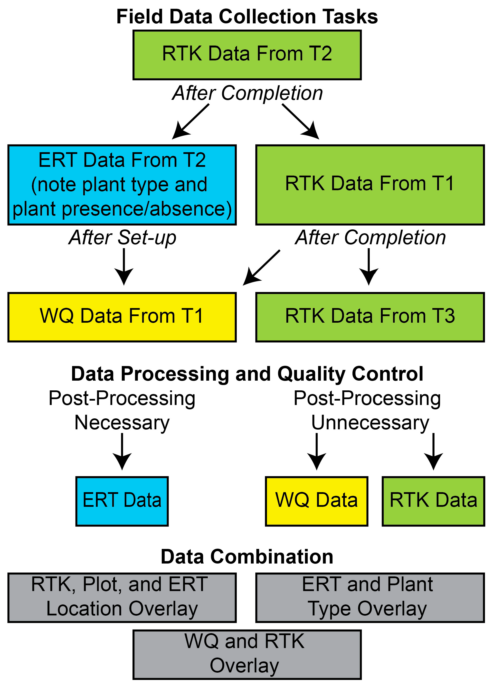
2.2. Data Collection and Processing

Figure 2 shows the data collection, data processing, and data overlay flowchart. During each field site visit, ground elevations along all transects were surveyed every 5 to 10 m from the marsh upland to the creek bank. A Trimble R8 RTK GPS receiver was used to collect these data. The RTK data had vertical and horizontal accuracies of 0.020 and 0.0010 m, respectively, and are reported as the root mean square (RMS) error (68% confidence level) [28]. RTK data are in the NAD83 UTM Zone 17 horizontal coordinate system (EPSG 26917), and elevations are NAVD 88 orthometric heights (in meters) computed using the National Geodetic Survey GEOID 12A. All RTK data were collected within two hours of low tide. RTK data are real-time and are not post-processed.
After RTK measurements were complete (Figure 2), water quality data were collected from T1 plots (green triangles in Figure 1B–D) within two hours of low tide using a 90 cm long push-point piezometer (MHE Products) coupled to a peristaltic pump (Geotech Environmental Equipment, Inc., Denver, CO, USA) and measured with a YSI-Xylem EXO1 water quality meter (Table 3). The water quality meter was calibrated to factory-supplied solutions following manufacturer specifications before each field sampling session. The metal push-point piezometer has a 5 cm screen length and a 0.5 cm inner diameter. Water was typically drawn from 90 cm depth but was occasionally drawn from shallower depths (Table 3) if 90 cm depth yielded inadequate water for measurement. All water quality data were collected after >500 mL of water (>3 times the piezometer volume) was purged from the piezometer, and water quality parameters were stabilized.
After RTK data were collected (Figure 2), bulk resistivity was measured concurrently with water quality data. To avoid interference between metal piezometers and resistivity measurements, ERT data were collected from T2 (yellow line in Figure 1B–D). To image bulk resistivity, two-dimensional electrical resistivity profiles were collected during daylight hours. A stationary eight-channel, 168 m long SuperSting R8/IP Marine Electrical Resistivity Meter equipped with 56 electrodes spaced 3 m apart (Advanced Geosciences, Inc., Austin, TX, USA) was used to collect the bulk resistivity data. Before collecting data, we tested the receiver, relay, and cable to verify optimal equipment functioning. After equipment checks, the cable was positioned shore perpendicular in a straight line to image as much of the dieback area as possible, with any remainder of the cable extending toward the nearest creek. At all sites, the length of the marsh platform exceeded the cable length. A sandbag was placed atop each electrode to optimize contact resistance. Contact resistance checks ensured values were typically below 100 ohm-m. All data were collected using a dipole-dipole array with a strong gradient to maximize the signal-to-noise ratio. The dipole-dipole array was selected because of its horizontal and vertical exploration capabilities, ability to resolve near-surface features, and potential to detect lateral resistivity variations [29,30]. This ERT configuration has a 3.0 m horizontal resolution and a 1.0 m vertical resolution near the Earth’s surface, increasing to 4.5 m horizontal and 1.5 m vertical resolution with depth. When time allowed, time-series resistivity profiles were collected on the same day but at tide conditions ranging from low to high tide. These surveys provide information about temporal and spatial changes in the marsh platform [18]. We also recorded the presence or absence of marsh grasses at each electrode. Depression storage of surface water on the marsh platform was always minimal, as were elevation changes along the profile.
All measured apparent resistivity profiles were processed identically using Earth Imager 2D, which uses Gauss–Newton and quasi-Newton methods (Advanced Geosciences, Inc.). Inversion parameters were set to default values for smooth inversion and included data spike removal [31]. The inversion parameters were set to allow no more than seven model iterations; however, all profiles converged in three iterations. The inversion process was considered converged when RMS was <6% and L2-norm was less than 1 [31,32]. RMS represents the difference between the calculated and measured apparent resistivity values [33] in the profile, while L2-norm is a smoothness constraint that measures data misfit between observed and predicted data [31,32].

3. Results

At the beginning of the study, the median intertidal elevation of the marsh platform was 0.72, 0.70, and 0.58 m relative to the NAVD 88 for GC, SSI, and PP, respectively (Table 1). Elevation changes across the platform from the upland border to the creek bank for each site ranged from 0.88, 2.28, and 1.45 m for GC, SSI, and PP, respectively (Table 1). The lowest elevations were near creek banks, where tall S. alterniflora was found, and the highest elevations were along the upland border. Similar average water salinity existed across the marsh platform (A, E, and H condition classes) within each site (Figure 3). PP had the least saline water (range 15.5–32.2, average ± standard deviation 22.2 ± 4.3, n = 15), followed by GC (range 18.5–37.5, 26.2 ± 5.8, n = 17), and then SSI (range 27.5 to 38.3, 33.6 ± 3.1, n = 14), as shown in Table 3. Approximate specific conductivities and resistivities for these waters are also shown in Figure 3.
The ERT cable was placed in the same location along T2 for both collection dates, and the data collection and inversion parameters were held constant over time. Thus, changes in resistivity across different sampling times resulted from changes in water chemistry [18]. The cable straddled the dieback areas at the SSI and PP sites (Figure 4C–F). The dieback extended beyond the cable length (Figure 4A,B) at GC. The ERT profiles from all sites showed consistent subsurface characteristics for October and March (Figure 4A–F) and through ebb-to-flood tide conditions (not shown). During the modeling process, the electrodes closest to the upland border (horizontal distance = 162 m) at all sites typically had lower contact resistance than electrodes closer to the creek. All data from all sites were processed with RMS varying between 3.75 and 5.64% and L2-norm varying between 0.44 and 0.74 (Figure 4A–F). These statistics are well within model acceptance tolerances [19]. All models had low overall resistivities, with PP having the highest maximum resistivity of 8.1 ohm-m (Figure 4E,F), followed by GC at 4.8 ohm-m (Figure 4A,B) and SSI at 2.0 ohm-m (Figure 4C,D).
Generally speaking, all sites showed consistent resistivity at shallow depths across each transect regardless of plant species and dieback status (Figure 4A,F). Although the resistivity scales vary between sites, several generalizations regarding the ERT data can be made. Bulk resistivity within the top ~0.8 m of the platform (green hues) at all sites was similar to the bulk resistivity at depths ranging from ~5 to ~6.5 m for GC and PP and from ~5 to ~13 m for SSI (Figure 4A–F). Between ~0.8 and ~5 m depth, bulk resistivity decreased to its lowest values, indicated by blue hues in Figure 4A–F. Bulk resistivity increased to its highest values (yellow, orange, and red hues) below ~6.5 m at the GC and PP sites and below ~13 m at the SSI site (Figure 4A–F).

4. Discussion

ERT models produce non-unique solutions from inherent limitations in the inversion process, which relies on a finite number of electrodes [30]. This characteristic allows for multiple resistivity models that fit the observed data while adhering to data accuracy constraints [34]. Additionally, as data density decreases with increasing depth, the potential for alternative solutions increases, further reducing model constraints, particularly at depth [32,35]. While the horizontal and vertical resolution of the ERT method smooths and averages the resistivity signal, the data nevertheless suggest a coherent interpretation of the shallow hydrostratigraphy beneath all three marsh platforms.
For all sites, the ERT data suggest a hydrostratigraphic sequence starting with a layer of low permeability unsaturated mud and peat from the surface down to ~0.8 m depth, shown as green hues in Figure 4A–F. Biological processes such as root growth, organic matter decomposition, and fiddler crab burrows occur within this unsaturated zone [14,36]. At shallow depths, Hemond and Fifield [37] hypothesized that evapotranspiration could lead to a cascade of events, including air entry into shallow marsh muds through crab burrows and old root channels. Dense mats of S. alterniflora roots, rhizomes, and aerenchyma modify the physical structure of the shallow subsurface and contribute to an environment conducive to air trapping and enhanced aeration [38]. Li et al. [39] also demonstrated that during inundation, air can become trapped in finer marsh soils, such as silt and clay. Xin et al. [40] further suggested that crab burrows can increase water flow and enhance aeration. Enhanced aeration, trapped air, and root networks act as insulators, increasing bulk resistivity compared to saturated materials [41]. The bulk resistivities at <0.8 m depth observed across each platform at all three field sites (green hues in Figure 4A–F) are consistent with these hypotheses.
Below the unsaturated zone, the marsh hydrostratigraphic sequence at all sites indicated a resistivity change at ~0.8 m depth, transitioning to the lowest measured resistivity values (0.2 to 0.4 ohm-m), represented by blue hues in Figure 4A–F. We interpret this change as the top of the water table, which is located near the Earth’s surface, where the ERT resolution is higher due to the greater density of current paths. Although this depth is shallower than the vertical resolution of the ERT data, this interpretation is supported by field measurements from piezometers, which consistently yielded water from depths of 0.9 m and occasionally shallower (Table 3). These measurements also align with the expected location of the water table, which fluctuates around the mean sea level (MSL; Figure 4A–F). Both the piezometer data and the alignment with MSL provide ground-truth validation for the resistivity interpretation.
Since water is conductive, its presence reduces bulk resistivity. Consequently, the lowest resistivity values indicate marsh muds or mud–sand mixtures saturated with brackish water or saltwater [42] at ~0.8 m depth. The lower salinities observed at PP are consistent with its higher resistivity values compared to the other sites (Table 1). These findings align with previous studies, where resistivity values below 2.5 ohm-m typically indicate marine sediments saturated with seawater, while higher resistivity values suggest marine sediments saturated with brackish or freshwater [43]. The ERT data suggest that this saturated zone forms a continuous, unconfined aquifer in marsh muds at all sites (Figure 4A–F). During site visits, water extracted from the piezometer was often mixed with air. We do now know the definitive source of the air; however, possibilities include air trapped in the marsh during flooding [37,38,39], biogenic gas [44], or air resulting from reduced inflow rates during sampling. As expected, given the distance from the creek, no slope of the water table toward the creek bank was observed, as each profile was collected at least 47 m from the nearest creek (Table 1).
Below ~5 m depth, each site exhibited a gradual increase in resistivity represented by green, then yellow, orange, and finally red hues. This pattern suggests that, with increasing depth, salty water may gradually change to brackish water, that sandy materials associated with a confined aquifer may become more prevalent, and that greater sediment compaction decreased porosity [42]. At greater depths, Harvey et al. [45] hypothesize that fine decomposed organic matter could fill pore spaces within sandy strata, reducing porosity. As resistivity is inversely related to porosity and the conductivity of the fluids [42], this reduction in porosity would result in increased resistivity. The observed pattern of increasing resistivity with depth (Figure 4A–F) aligns with this hypothesis. Additionally, the consistently low bulk resistivity values (max of 8.1 ohm-m) across all sites suggest that brackish water is likely present at depth at each site [42], with PP being the least saline site (Figure 3).
The ERT data provide valuable insights, but overlapping resistivity ranges and the absence of sediment core data reduce the interpretability of bulk resistivity in the deeper sections of the salt marshes. Nevertheless, the typical stratigraphy of marshes in the southeastern United States often consists of 1 to 4 m of fine-grained marsh mud overlying sandy layers, of which all materials are Quaternary in age [4,14,46,47,48,49,50]. These sandy layers are frequently relict beach ridge deposits or sandy tidal channel deposits [47]. They function as confined aquifers and serve as conduits for groundwater flow from upland marsh areas to tidal creeks [45,49].
At the SSI site (Figure 4C,D), a notable resistivity feature is characterized by light green hues. This feature extends 9 m horizontally, between 60 and 69 m horizontal distance, and vertically from a depth of 4.9 to 14.7 m (approximately 10 m tall). This feature is positioned beneath the dieback-affected area of the marsh but does not connect to any distinguishing characteristic on the marsh surface (Figure 1C). The exact nature of this feature remains inconclusive without additional data. This feature also connects to a shallower, higher-resistivity zone, indicated by yellow and orange hues, that is located at horizontal distances of 15 to 60 m and depths of 6 to 10 m. This shallower feature may represent a higher permeability zone that facilitates water movement beneath the marsh toward the creek. Such a zone could consist of a sandy layer interspersed within the presumably predominantly fine-grained muddy substrate. Alternatively, this feature may be associated with higher resistivity less-saline water movement, a plausible interpretation if the stratigraphy consists predominantly of homogeneous fine-grained materials. Additionally, the ERT data from the SSI site suggest the presence of a brackish lens at the upland border between horizontal distances of 156 to 162 m and depths of 0 and 5 m (Figure 4C,D). This lens is depicted by yellow and orange hues (Figure 4C,D). A recently installed 90 cm deep well at the upland border yielded water with an average salinity of 3.7, supporting the growth of B. frutescens, a species that prefers fresher water environments [51]. However, we cannot rule out that this resistivity feature could be related to fill material associated with the adjacent F.J. Torras Causeway. The causeway directly abuts the upland border plots, which are outside of the scope of this study and are not shown in Figure 1C. Notably, both the vertical conduit and upland border resistivity features are absent from the GC and PP sites.
At the PP site, a ~1 m wide, shallow creek is located between horizontal distances of 147 and 150 m (Figure 1D and Figure 4E,F). Although this creek held water at low tide during data collection, it is not visible in the ERT profiles. Another small creek was forming between horizontal distances of 78 and 84 m (Figure 1D), but this creek also does not appear in the ERT data (Figure 4E,F). Additionally, J. roemerianus was present in the ERT profile between horizontal distances of 99 and 129 m (Figure 1D); however, there was no detectable difference in the hydrostratigraphy beneath J. roemerianus compared to S. alterniflora (Figure 4E,F). The ERT profiles reveal the highest overall resistivity (8.1 ohm-m) at the PP field site, suggesting the presence of less saline groundwater compared to GC and SSI. This result aligns with the presence of a large stand of J. roemerianus, which typically indicates systems with fresher water conditions [52].
Our sampling protocol involved collecting water quality data along T1 and ERT data along T2. This approach created a limitation for data interpretation because the shallow ground truth measurements (Table 3) were not collected directly underneath the cable. However, average salinities for all condition classes at each field site were not significantly different (repeated measures ANOVA, F2,40 = 0.611, p = 0.574; Figure 3), suggesting similar water quality parameters across the platform of the marsh through time. Thibodeau [53] also found little variation in the salinity spatial pattern over time at a marsh site in South Carolina. Several studies [53,54,55] found lower salinities in their respective salt marsh field sites during the winter months when rainfall was higher and evapotranspiration rates were lower compared to summer months. Except for PP (Table 3), our field data do not suggest a similar relationship (repeated measures ANOVA, F1,34 = 0.044, p = 0.845), though there was a significant interaction between site and season (p = 0.00108). However, note that our sampling protocol was limited to one data point seasonally for only two years, making statistical inferences difficult.
Flooding of the marsh platform during tidal inundation is the dominant driver of the saturation state [56], and therefore, groundwater resistivity changes. Thus, it is unsurprising that the precipitation (Table 2) prior to collecting ERT profiles did not noticeably impact the bulk resistivity measurements. The bulk resistivity at depth also remained similar at each field site over time. This is likely due to the predictable tidal flooding regime at the field sites, which creates predictable groundwater flow regimes [57]. The ERT data also show little variation across seasons, suggesting that seasonal changes do not greatly impact the groundwater conductivity at any of the study sites. Collectively, the frequent and dominant tidal flushing signature of the platform might obscure any such relationships if they exist. Alternatively, while the ERT profiles image relatively deep beneath the marsh platform, the observed similarities may suggest that, at the horizontal and vertical resolution of the ERT data, the data are insufficient to detect changes in soil aeration conditions. This limitation includes macroporosity from crab burrows and roots, as well as crab burrow density. Furthermore, the ERT data are insufficient to detect changes in water conductivity resulting from evapotranspiration in the root zone, as observed by field researchers [37,58]. Alternatively, such signatures may be masked by the tidal signal, as suggested by Thibodeau [53].
The ERT data across the marsh platform were similar beneath all three vegetation condition classes (dieback, affected, and healthy; Figure 4A–F). Furthermore, we detected no changes to the shallow hydrostratigraphy as the marsh vegetation began recolonizing the dieback areas during the period of dieback recovery between the October 2015 and March 2016 ERT collection dates (Figure 4A–F). Additionally, changes in vegetation type or marsh dieback and recovery status do not appear to be affected by depth to groundwater. However, any potential relationships between initial dieback and resistivity would have been missed as our sampling occurred well after the onset of dieback.
We found that vegetation species followed a general zonation pattern across the topographical gradient from low to high marsh. Observed plant distributions corresponded to those previously described [59] for Southeastern salt marshes with tall S. alterniflora at lower elevations and J. roemerianus and B. frutescens at higher elevations. McKee and Patrick [60] found that species elevations can vary widely among salt marshes, making elevation comparisons difficult between marsh sites. The mean RTK elevation and range for each site correspond with previous observations in Georgia salt marshes [61,62]. However, despite the elevation difference among the studied marsh sites, we did not detect corresponding changes in bulk resistivity, suggesting that elevation may not influence resistivity patterns.
ERT profiles show similar bulk resistivities across different tidal heights at each field site, suggesting that the profiles were collected too far from the creek to detect tidally driven groundwater flow or depth to any mud/sand contact at the creek bank. The cable was positioned 56, 51, and 47 m from the low tide line of the creek at GC, SSI, and PP, respectively (Table 1). Several studies have modeled [48,56,57,63] or measured [64,65] groundwater flow and tidal signal propagation from the creek for various marsh geometries in the southeastern United States. Except for storm-driven groundwater flow [48], these studies generally agree that groundwater flow typically occurs within 2 to 15 m of the creek, and tidal signal propagation into the marsh platform rarely exceeds 35 m from the creek. Thus, the ERT results align with previously published models and field data.
Finally, the deployment of the ERT cable on the marsh had ecological consequences. Despite our efforts to minimize disturbance, the process left a visible path through the marsh due to the large crew required to deploy the equipment. This resulted in unintended damage to vegetation and soil structure. Based on our experience and the consistent ERT results obtained at each field site, we recommend conducting only one ERT survey at any given marsh site with the smallest crew possible to minimize ecological impact.

5. Conclusions

This study used multichannel ERT surveys to identify subsurface resistivity patterns beneath three salt marshes. The results for all sites suggest typical marsh hydrostratigraphy consisting of unsaturated mud and peat overlying an unconfined muddy aquifer saturated with saltwater. There is minimal evidence of freshwater influence. We established that the ERT data reveal consistent subsurface resistivity patterns across seasons and tidal flooding. Bulk resistivity patterns were similar under S. alterniflora and J. roemerianus. Further, all three marsh vegetation condition classes (healthy, affected, dieback) showed similar bulk resistivity patterns. Vegetation status, seasonal changes, and tidal variation had minimal influence on water depth or chemistry, suggesting that tidal flooding predominantly governs shallow subsurface dynamics in these marshes. Our findings suggest that the processes driving the recovery of marsh dieback are independent of the shallow marsh stratigraphy. These findings contribute to a better understanding of salt marsh subsurface conditions and the role they play in marsh resilience and dieback recovery, informing future studies on the hydrological factors influencing marsh health.

Author Contributions

Conceptualization, J.L.K. and C.M.H.; methodology, J.L.K. and C.M.H.; investigation, J.L.K. and C.M.H.; resources, J.L.K. and C.M.H.; data curation, J.L.K. and C.M.H.; writing—original draft preparation, J.L.K. and C.M.H.; writing—review and editing, J.L.K. and C.M.H.; project administration, J.L.K. and C.M.H.; funding acquisition, J.L.K. and C.M.H. All authors have read and agreed to the published version of the manuscript.

Funding

This research was funded under grant award #NA15NOS4190160 to the Department of Natural Resources from the Office of Ocean and Coastal Resource Management, National Oceanic and Atmospheric Administration. The statements, findings, conclusions, and recommendations are those of the authors and do not necessarily reflect the views of DNR, OCRM, or NOAA.

Data Availability Statement

Some data for the St. Simons Island field site are openly available in interactive form via a Story Map titled “A Case Study on Salt Marsh Dieback”, which is available online at: https://storymaps.arcgis.com/stories/aabb57ed8a524e9f8a0d56b129d41460 (accessed on 3 January 2025). The raw data supporting the conclusions of this article will be made available by the authors on request.

Acknowledgments

We thank the many students from Georgia Southern University who helped us collect the data presented herein. We thank the Coastal Resources Division and Jan Mackinnon for their help with selecting field sites. Comments by two anonymous reviewers greatly improved this manuscript.

Conflicts of Interest

The authors declare no conflicts of interest.

References

  1. Costanza, R.; d’Arge, R.; de Groot, R.; Farber, S.; Grasso, M.; Hannon, B.; Limburg, K.; Naeem, S.; O’Neill, R.V.; Paruelo, J.; et al. The value of the world’s ecosystem services and natural capital. Nature 1997, 387, 253–260. [Google Scholar] [CrossRef]
  2. Mitsch, W.J.; Gosselink, J.G. Wetlands, 3rd ed.; John Wiley and Sons: Hoboken, NJ, USA, 2000. [Google Scholar]
  3. Elsey-Quirk, T.; Lynn, A.; Jacobs, M.D.; Diaz, R.; Cronin, J.; Wang, L.; Huang, H.; Justic, D. Vegetation dieback in the Mississippi River Delta triggered by acute drought and chronic relative sea-level rise. Nat. Commun. 2024, 15, 3518. [Google Scholar] [CrossRef] [PubMed]
  4. Hughes, A.L.; Wilson, A.M.; Morris, J.T. Hydrologic variability in a salt marsh: Assessing the links between drought and acute marsh dieback. Estuar. Coast. Shelf Sci. 2012, 111, 95–106. [Google Scholar] [CrossRef]
  5. Marsh, A.; Blum, L.K.; Christian, R.R.; Ramsey III, E.; Rangoonwala, A. Response and resilience of Spartina alterniflora to sudden dieback. J. Coast. Conserv. 2016, 20, 335–350. [Google Scholar] [CrossRef]
  6. Morton, R.A.; Tiling, G.; Ferina, N.F. Causes of hot-spot wetland loss in the Mississippi delta plain. Environ. Geosci. 2003, 10, 71–80. [Google Scholar] [CrossRef]
  7. Schepers, L.; Kirwan, M.; Guntenspergen, G.; Temmerman, S. Spatio-temporal development of vegetation die-off in a submerging coastal marsh. Limnol. Oceanogr. 2017, 62, 137–150. [Google Scholar] [CrossRef]
  8. Alber, M.; Swenson, E.M.; Adamowicz, S.C.; Mendelssohn, I.A. Salt marsh dieback: An overview of recent events in the US. Estuar. Coast. Shelf Sci. 2008, 80, 1–11. [Google Scholar] [CrossRef]
  9. Ogburn, M.B.; Alber, M. An investigation of salt marsh dieback in Georgia using field transplants. Estuaries Coasts 2006, 29, 54–62. [Google Scholar] [CrossRef]
  10. Day, J.W.; Christian, R.R.; Boesch, D.M.; Yáñez-Arancibia, A.; Morris, J.; Twilley, R.R.; Naylor, L.; Schaffner, L.; Stevenson, C. Consequences of Climate Change on the Ecogeomorphology of Coastal Wetlands. Estuaries Coasts 2008, 31, 477–491. [Google Scholar] [CrossRef]
  11. Baustian, J.J.; Mendelssohn, I.A.; Hester, M.W. Vegetation’s importance in regulating surface elevation in a coastal salt marsh facing elevated rates of sea level rise. Glob. Change Biol. 2012, 18, 3377–3382. [Google Scholar] [CrossRef]
  12. Coleman, D.J.; Kirwan, M.L. The effect of a small vegetation dieback event on salt marsh sediment transport. Earth Surf. Process. Landf. 2019, 44, 944–952. [Google Scholar] [CrossRef]
  13. Krest, J.M.; Moore, W.S.; Gardner, L.R.; Morris, J.T. Marsh nutrient export supplied by groundwater discharge: Evidence from radium measurements. Glob. Biogeochem. Cycles 2000, 14, 167–176. [Google Scholar] [CrossRef]
  14. Morris, J.T.; Sundareshwar, P.V.; Nietch, C.T.; Kjerfve, B.; Cahoon, D.R. Responses of coastal wetlands to rising sea level. Ecology 2002, 83, 2869–2877. [Google Scholar] [CrossRef]
  15. Materne, M.; Bush, T.; Houck, M. Plant Guide for Smooth Cordgrass (Spartina alterniflora). USDA-Natural Resources Conservation Service. 2022. Available online: https://www.nrcs.usda.gov/plantmaterials/njpmcpg13933.pdf (accessed on 3 January 2025).
  16. Eleuterius, L.N. Vegetative Morphology and Anatomy of the Salt Marsh Rush, Juncus roemerianus. Gulf Res. Rep. 1976, 5, 1–10. [Google Scholar] [CrossRef]
  17. Moore, W.S.; Blanton, J.O.; Joye, J. Estimates of flushing times, submarine groundwater discharge, and nutrient fluxes to Okatee Estuary, South Carolina. J. Geophys. Res. 2006, 111, C09006. [Google Scholar] [CrossRef]
  18. Swarzenski, P.W.; Izbicki, J.A. Coastal groundwater dynamics off Santa Barbara, California: Combining geochemical tracers, electromagnetic seepmeters, and electrical resistivity. Estuar. Coast. Shelf Sci. 2009, 83, 77–89. [Google Scholar] [CrossRef]
  19. Dimova, N.T.; Swarzenski, P.W.; Dulaiova, H.; Glenn, C.R. Utilizing multichannel electrical resistivity methods to examine the dynamics of the fresh water-seawater interface in two Hawaiian groundwater systems. J. Geophys. Res. 2012, 117, C02012. [Google Scholar] [CrossRef]
  20. Swarzenski, P.W.; Burnett, W.C.; Greenwood, W.J.; Herut, B.; Peterson, R.; Dimova, N.; Shalem, Y.; Yechieli, Y.; Weinstein, Y. Combined time-series resistivity and geochemical tracer techniques to examine submarine groundwater discharge at Dor Beach, Israel. Geophys. Res. Lett. 2006, 33, L24405. [Google Scholar] [CrossRef]
  21. U.S. Climate Data. Available online: https://www.usclimatedata.com/ (accessed on 13 November 2024).
  22. Wiegert, R.G.; Pomeroy, L.R.; Wiebe, W.J. Ecology of salt marshes: An introduction. In The Ecology of a Salt Marsh; Pomeroy, L.R., Wiegert, R.G., Eds.; Springer: New York, NY, USA, 1981; pp. 3–19. [Google Scholar]
  23. Tides and Currents (Datums for 8670870, Fort Pulaski GA). Available online: https://tidesandcurrents.noaa.gov/datums.html?datum=MLLW&units=1&epoch=0&id=8670870&name=Fort+Pulaski&state=GA (accessed on 13 November 2024).
  24. Tides and Currents (Datums for 8720030, Fernandina Beach FL). Available online: https://tidesandcurrents.noaa.gov/datums.html?datum=MLLW&units=1&epoch=0&id=8720030&name=Fernandina+Beach&state=FL (accessed on 13 November 2024).
  25. Tides and Currents (Relative Sea Level Trend Fort Pulaski). Available online: https://tidesandcurrents.noaa.gov/sltrends/sltrends_station.shtml?id=8670870 (accessed on 13 November 2024).
  26. Tides and Currents (Relative Sea Level Trend Fernandina Beach). Available online: https://tidesandcurrents.noaa.gov/sltrends/sltrends_station.shtml?id=8720030 (accessed on 13 November 2024).
  27. Dibble, M. Examination of Salt Marsh Dieback Development and Recovery Using Historical Aerial Photography and Climatic Conditions. Bachelor’s Thesis, Georgia Southern University, Statesboro, GA, USA, 2017. [Google Scholar]
  28. Trimble R8 GNSS Receiver User Guide. Available online: https://trl.trimble.com/docushare/dsweb/Get/Document-666215/R8-R6-5800_v400A_UserGuide.pdf (accessed on 23 July 2024).
  29. Rinaldi, V.; Guichon, M.; Ferrero, V.; Serrano, C.; Ponti, N. Resistivity Survey of the Subsurface Conditions in the Estuary of the Rio de la Plata. J. Geotech. Geoenviron. Eng. 2006, 132, 72–79. [Google Scholar] [CrossRef]
  30. Loke, M.H.; Chambers, J.E.; Rucker, D.F.; Kuras, O.; Wilkinson, P.B. Recent developments in the direct-current geoelectrical imaging method. J. Appl. Geophys. 2013, 95, 135–156. [Google Scholar] [CrossRef]
  31. Advanced Geosciences Incorporated Instruction Manual for EarthImager 2D Resistivity and IP Inversion Software. Available online: http://www.agiusa.com/ (accessed on 13 November 2024).
  32. Nguyen, F.; Garambois, S.; Jongmans, D.; Pirard, E.; Loke, M.H. Image processing of 2D resistivity data for imaging faults. J. Appl. Geophys. 2005, 57, 260–277. [Google Scholar] [CrossRef]
  33. Caputo, R.; Piscitelli, S.; Oliveto, A.; Rizzo, E.; Lapenna, V. The use of electrical resistivity tomographies in active tectonics: Examples from the Tyrnavos Basin, Greece. J. Geodyn. 2003, 36, 19–35. [Google Scholar] [CrossRef]
  34. Hoffmann, R.; Dietrich, P. An approach to determine equivalent solutions to the geoelectrical 2D inversion problem. J. Appl. Geophys. 2004, 56, 79–91. [Google Scholar] [CrossRef]
  35. Oldenburg, D.W.; Li, Y. Estimating depth of investigation in dc resistivity and IP surveys. Geophysics 1999, 64, 403–416. [Google Scholar] [CrossRef]
  36. Michaels, R.E.; Zieman, J.C. Fiddler crab (Uca spp.) burrows have little effect on surrounding sediment oxygen concentrations. J. Exp. Mar. Biol. Ecol. 2013, 448, 104–113. [Google Scholar] [CrossRef]
  37. Hemond, H.F.; Fifield, J.L. Subsurface flow in salt marsh peat: A model and field study. Limnol. Oceanogr. 1982, 27, 126–136. [Google Scholar] [CrossRef]
  38. Granse, D.; Titschack, J.; Ainouche, M.; Jensen, K.; Koop-Jackobsen, K. Subsurface aeration of tidal wetland soils: Root-system structure and aerenchyma connectivity in Spartina (Poaceae). Sci. Total Environ. 2022, 802, 149771. [Google Scholar] [CrossRef]
  39. Li, H.; Li, L.; Lockington, D. Aeration for plant root respiration in a tidal marsh. Water Resour. Res. 2005, 41, W06023. [Google Scholar] [CrossRef]
  40. Xin, P.; Jin, G.; Li, L.; Barry, D.A. Effects of crab burrows on pore water flows in salt marshes. Adv. Water Resour. 2009, 32, 439–449. [Google Scholar] [CrossRef]
  41. Silva Filho, A.M.; Silva, J.R.S.; Fernandes, G.M.; Morais, L.D.; Coimbra, A.P.; Calixto, W.P. Root system analysis and influence of moisture on soil electrical properties. Energies 2021, 14, 6951. [Google Scholar] [CrossRef]
  42. Archie, G.E. The Electrical Resistivity Log as an Aid in Determining Some Reservoir Characteristics. Trans. AIME 1942, 146, 54–62. [Google Scholar] [CrossRef]
  43. Papen, M.; Hanssens, D.; De Smedt, P.; Walraevens, K.; Hermans, T. Combining resistivity and frequency domain electromagnetic methods to investigate submarine groundwater discharge in the littoral zone. Hydrol. Earth Syst. Sci. 2020, 24, 3539–3555. [Google Scholar] [CrossRef]
  44. Koontz, E.L.; Parker, S.M.; Stearns, A.E.; Roberts, B.J.; Young, C.M.; Windham-Myers, L.; Oikawa, P.Y.; Megonigal, J.P.; Noyce, G.L.; Buskey, E.J.; et al. Controls on spatial variation in porewater methane concentrations across United States tidal wetlands. Sci. Total Environ. 2024, 957, 177290. [Google Scholar] [CrossRef] [PubMed]
  45. Harvey, J.W.; Germann, P.F.; Odum, W.E. Geomorphological control of subsurface hydrology in the creekbank zone of tidal marshes. Estuar. Coast. Shelf Sci. 1987, 25, 677–691. [Google Scholar] [CrossRef]
  46. Gardner, L.R.; Porter, D.E. Stratigraphy and geologic history of a southeastern salt marsh basin, North Inlet, South Carolina, USA. Wetl. Ecol. Manag. 2001, 9, 371–385. [Google Scholar] [CrossRef]
  47. Gardner, L.R. Role of stratigraphy in governing pore water seepage from salt marsh sediments. Water Resour. Res. 2007, 43, W07502. [Google Scholar] [CrossRef]
  48. Wilson, A.M.; Moore, W.S.; Joye, S.B.; Anderson, J.L.; Schutte, C.A. Storm-driven groundwater flow in a salt marsh. Water Resour. Res. 2011, 47, W02535. [Google Scholar] [CrossRef]
  49. Wilson, A.M.; Evans, T.; Moore, W.; Schutte, C.A.; Joye, S.B.; Hughes, A.H.; Anderson, J.L. Groundwater controls ecological zonation of salt marsh macrophytes. Ecology 2015, 96, 840–849. [Google Scholar] [CrossRef]
  50. Alexander, C.R.; Hodgson, J.Y.S.; Brandes, J.A. Sedimentary processes and products in a mesotidal salt marsh environment: Insights from Groves Creek, Georgia. Geo-Mar. Lett. 2017, 37, 345–359. [Google Scholar] [CrossRef]
  51. Lonard, R.I.; Judd, F.W.; Stalter, R. Biological flora of coastal dunes and wetlands: Borrichia frutescens (L.) DC. J. Coast. Res. 2015, 31, 749–757. [Google Scholar] [CrossRef]
  52. Pennings, S.C.; Grant, M.-B.; Bertness, M.D. Plant zonation in low-latitude salt marshes: Disentangling the roles of flooding, salinity and competition. J. Ecol. 2005, 93, 159–167. [Google Scholar] [CrossRef]
  53. Thibodeau, P.M.; Gardner, L.R.; Reeves, H.W. The role of groundwater flow in controlling the spatial distribution of soil salinity and rooted macrophytes in a southeastern salt marsh, USA. Mangroves Salt Marshes 1998, 2, 1–13. [Google Scholar] [CrossRef]
  54. Gardner, L.R.; Reeves, H.W. Seasonal patterns in the soil water balance of a Spartina marsh site at North Inlet, South Carolina, USA. Wetlands 2002, 22, 467–477. [Google Scholar] [CrossRef]
  55. Montalvo, M.S.; Grande, E.; Graswell, A.E.; Visser, A.; Arora, B.; Seybold, E.C.; Tatariw, C.; Haskiins, J.C.; Endris, C.A.; Gerbl, F.; et al. A Fresh Take: Seasonal Changes in Terrestrial Freshwater Inputs Impact Salt Marsh Hydrology and Vegetation Dynamics. Estuaries Coasts 2024, 47, 2389–2405. [Google Scholar] [CrossRef]
  56. Wilson, A.M.; Morris, J.T. The influence of tidal forcing on groundwater flow and nutrient exchange in a salt marsh-dominated estuary. Biogeochemistry 2012, 108, 27–38. [Google Scholar] [CrossRef]
  57. Wilson, A.M.; Gardner, L.R. Tidally driven groundwater flow and solute exchange in a marsh: Numerical simulations. Water Resour. Res. 2006, 42, W01405. [Google Scholar] [CrossRef]
  58. Xin, P.; Gibbes, B.; Ling, L.; Song, Z.; Lockington, D. Soil saturation index of salt marshes subjected to spring-neap tides: A new variable for describing marsh soil aeration condition. Hydrol. Process. 2010, 24, 2564–2577. [Google Scholar] [CrossRef]
  59. Wiegert, R.G.; Freeman, B.J. Tidal Salt Marshes of the Southeast Atlantic Coast: A Community Profile; U.S. Department of the Interior, Fish and Wildlife Service: Washington, DC, USA, 1990. [CrossRef]
  60. McKee, K.L.; Patrick, W.H., Jr. The relationship of smooth cordgrass (Spartina alterniflora) to tidal datums: A review. Estuaries 1988, 11, 143–151. [Google Scholar] [CrossRef]
  61. Hladik, C.M.; Alber, M.; Schalles, J.F. Salt marsh elevation and habitat mapping using hyperspectral and LIDAR data. Remote Sens. Environ. 2013, 139, 318–330. [Google Scholar] [CrossRef]
  62. Hladik, C.; Alber, M. Accuracy assessment and correction of a LIDAR-derived salt marsh digital elevation model. Remote Sens. Environ. 2012, 121, 224–235. [Google Scholar] [CrossRef]
  63. Gardner, L.R. Role of geomorphic and hydraulic parameters in governing pore water seepage from salt marsh sediments. Water Resour. Res. 2005, 41, W07010. [Google Scholar] [CrossRef]
  64. Schultz, G.; Ruppel, C. Constraints on hydraulic parameters and implications for groundwater flux across the upland-estuary interface. J. Hydrol. 2002, 260, 255–269. [Google Scholar] [CrossRef]
  65. Moffett, K.B.; Gorelick, S.M. Relating salt marsh pore water geochemistry patterns to vegetation zones and hydrologic influences. Water Resour. Res. 2016, 52, 1729–1745. [Google Scholar] [CrossRef]
Figure 1. (A) Site location map showing Grays Creek (GC) located at 32.030289° N, 81.037223° W, St. Simons Island (SSI) located at 31.165996° N, 81.441708° W, and Point Peter (PP) located at 30.759840° N, 81.531281° W field sites (yellow stars). The Fort Pulaski and Fernandina Beach tide stations (green circles) and the Savannah (SAV), Brunswick (BQK), and Fernandina Beach (FNB) weather stations (blue circles) are also shown. The weather stations are located within the boundaries of the cities of Savannah, Brunswick, and Fernandina Beach, respectively. Field site maps showing the plot locations (green triangles and plot labels), electrical resistivity cable placement (yellow line), and cable distances (blue dots and associated numbers) for (B) GC, (C) SSI, and (D) PP.
Water 17 00144 g001
Figure 2. Flowchart showing field data collection tasks, data processing, and quality control, as well as data combination tasks to create data overlays (gray boxes) for the real-time kinematic (RTK) elevation and location information (green boxes), the electrical resistivity tomography (ERT) bulk resistivity data (blue boxes), and the water quality (WQ) data (yellow boxes).
Water 17 00144 g002
Figure 3. Salinity, approximate specific conductivity, and approximate resistivity of the transect one (T1) plot at each field site relative to the distance from the creek. Error bars show the range of salinity values measured quarterly at each plot from November 2014 through July 2016. “H” indicates healthy plots, “E” indicates transitional edge plots, and “A” indicates affected (dieback) plots.
Water 17 00144 g003
Figure 4. Bulk electrical resistivity results for Gray’s Creek (GC) on (A) 9 October 2015 and (B) 4 March 2016; for St. Simons Island (SSI) on (C) 11 October 2015 and (D) 6 March 2016; and for Point Peter (PP) on (E) 10 October 2015 and (F) 5 March 2016. For all panels, the x-axis shows the distance across the marsh platform, with a distance of 0 m closest to the creek bank (but not at the creek bank) and a distance of 162 m at the upland border. The y-axis shows depth. All panels are displayed with a 0.85 vertical exaggeration with mean sea level (MSL) indicated on the x-axis of each panel. Model convergence parameters, including iterations, root mean square (RMS) error, and L2-norm, are shown in each panel. The coloration is a nonlinear electrical resistivity scale (ohm-m), which varies by site and was selected to maximize the resistivity scale for each location. Red hues represent higher bulk resistivity and lower conductivity compared to blue hues, which represent lower bulk resistivity and higher conductivity. Plant coverage is also shown along the x-axis, with the shorter light green plants representing Spartina alterniflora, the taller dark green plants representing Juncus roemerianus, and marsh dieback areas shown with no plant coverage. All panels correspond to low or nearly low tide conditions, as shown on the tidal stage insets. The tidal stage inset shows the time of day (M = Midnight and N = Noon) and tidal height (m) relative to mean lower low water (note, the y-axis scale changes from inset to inset). Tide data for GC were compiled from the Fort Pulaski station (#8670870), while tide data from SSI and PP were compiled from the Fernandina Beach station (#8720030).
Water 17 00144 g004
Table 1. Real-time kinematic summary statistics for transect two at each study site. Transects were measured from the upland border to the nearest creek, with elevations relative to the North American Vertical Datum 88. Refer to Figure 1B (Grays Creek), Figure 1C (St. Simons Island), and Figure 1D (Point Peter). Electrode 0 distance represents the closest point of the resistivity cable to the creek.
ParameterGrays Creek (GC)St. Simons
Island (SSI)
Point Peter (PP)
Minimum Elevation (m)0.03−0.50−0.48
Maximum Elevation (m)0.921.790.98
Elevation Change (m)0.882.281.45
Median Elevation (m)0.720.700.58
Mean Elevation (m)0.700.740.55
Standard Deviation (m)0.180.360.28
Transect Length (m)221216212
Electrode 0 Distance to Creek (m)565147
Table 2. Total precipitation and average tidal amplitude in the seven days prior to each field sampling date.
Sample DatePrecipitation (cm)Tidal Amplitude (m)
Gray’s Creek (GC)
10/09/20151.22.3
03/04/20161.71.8
St. Simons Island (SSI)
10/11/20150.41.9
03/06/20161.01.7
Point Peter (PP)
10/10/20153.01.7
03/05/20160.51.5
Table 3. Water quality data for the study sites were organized by plot and sample date. Depth is in centimeters, and specific conductivity (SPC) is in microsiemens per centimeter. Some plots did not always yield water and are indicated with “-”.
Sample DateDepthSalinitySPCDepthSalinitySPCDepthSalinitySPC
Grays CreekGC T1AGC T1EGC T1H
11/14/20144037.556,3293036.354,0503035.854,024
03/20/20159029.044,8019026.841,6509030.046,206
07/31/20159024.338,5809023.837,5909022.235,390
10/09/2015---9026.933,8549023.732,063
03/04/20169025.239,3799023.136,4389022.836,118
07/22/20169019.831,7669019.831,8209018.529,880
St. SimonsSSI T1ASSI T1ESSI T1H
11/01/20147035.653,8675033.751,1603032.649,761
03/21/20159038.355,2866034.451,8299036.652,648
07/25/20159035.253,7969027.542,8309031.348,200
10/11/20159036.048,002------
03/06/20169035.954,289------
07/24/20169034.151,8826030.947,5969028.644,410
Point PeterPP T1APP T1EPP T1H
11/02/20144020.332,4095015.525,2825017.027,629
03/28/20159026.942,6659032.254,1609022.535,562
07/26/20159025.039,4129022.836,0849018.424,773
10/10/2015---9022.838,1159023.0-
03/05/2016---9024.638,7109022.635,721
07/23/2016---9021.634,3009017.328,308
Disclaimer/Publisher’s Note: The statements, opinions and data contained in all publications are solely those of the individual author(s) and contributor(s) and not of MDPI and/or the editor(s). MDPI and/or the editor(s) disclaim responsibility for any injury to people or property resulting from any ideas, methods, instructions or products referred to in the content.

