Global Sensitivity Analysis of Slope Stability Considering Effective Rainfall with Analytical Solutions

Abstract

Rainfall-induced landslides are widely distributed in many countries. Rainfall impacts the hydraulic dynamics of groundwater and, therefore, slope stability. We derive an analytical solution of slope stability considering effective rainfall based on the Richards equation. We define effective rainfall as the total volume of rainfall stored within a given range of the unsaturated zone during rainfall events. The slope stability at the depth of interest is provided as a function of effective rainfall. The validity of analytical solutions of system states related to effective rainfall, for infinite slopes of a granite residual soil, is verified by comparing them with the corresponding numerical solutions. Additionally, three approaches to global sensitivity analysis are used to compute the sensitivity of the slope stability to a variety of factors of interest. These factors are the reciprocal of the air-entry value of the soil α, the thickness of the unsaturated zone L, the cohesion of soil c, the internal friction angle ϕ related to the effective normal stress, the slope angle β, the unit weights of soil particles γ_s, and the saturated hydraulic conductivity K_s. The results show the following: (1) The analytical solutions are accurate in terms of the relative differences between the analytical and the numerical solutions, which are within 5.00% when considering the latter as references. (2) The temporal evolutions of the shear strength of soil can be sequentially characterized as four periods: (i) strength improvement due to the increasing weight of soil caused by rainfall infiltration, (ii) strength reduction controlled by the increasing pore water pressure, (iii) strength reduction due to the effect of hydrostatic pressure in the transient saturation zone, and (iv) stable strength when all the soil is saturated. (3) The large α corresponds to high effective rainfall. (4) The factors ranked in descending order of sensitivity are as follows: α > L > c > β > γ_s > K_s > ϕ.

1. Introduction

Rainfall is the governing factor triggering landslides, especially in hilly and mountainous areas in China where annual atmospheric rainfall is high [1]. The recharge of rainfall to groundwater not only provides water for the ecosystem but also enhances the hydraulic dynamics of groundwater. The latter have negative impacts on slope stability, due to increases in the self-weight of a slope and decreases in soil strength [2,3,4]. The effects linked to the latter include increased water–rock interactions [5,6], decreased matrix suction [7], and increases in static water pressures [8,9,10,11].

There are many efforts devoted to exploring the factors influencing how slope stability is impacted by rainfall. These studies primarily concentrate on three aspects [12]: (i) the influence of soil-water characteristic curves and hydraulic parameters on the slope stability [13,14]; (ii) the spatiotemporal characteristics of slope wetting fronts [14,15]; and (iii) evaluation of the slope stability by integrating unsaturated shear strength and seepage theories [12,16,17]. The saturation of soil is the common system state of interest which has a significant influence on the slope stability. Specifically, the increase in the saturation of soil increases the self-weight of the slope, while decreasing the cohesion, matrix suction, and shear strength of soil. Nevertheless, the impacts of factors on the slope stability in a practical field case are still complicated and need to be further explored. Particularly, it is still unclear to which factor (and the corresponding physical process) and at which level the slope stability is most sensitive under the influence of rainfall. To answer these questions, a key element is to quantify how much water can be stored and work on the slope under a rainfall event of interest, which is linked to the concept of ‘effective rainfall’.

Crozier [18] first proposed the concept of effective rainfall in the field of landslides. It is defined as the total rainfall from the beginning of a rainfall event until the time of landslide deformation. Recently, this definition has been considered in several studies [19,20]. Kim et al. [19] analyzed the risk of landslides using the change in the volumetric water content of soil based on effective rainfall. Lee [20] conducted a study on the impact of effective rainfall on deep landslides. Effective rainfall is calculated utilizing rainfall intensity and the attenuation coefficient, the latter of which lacks a clear mathematical expression. Since the recharges (e.g., rainfall infiltration) and discharges (e.g., evapotranspiration) are spatiotemporal processes, the hydraulic dynamics of groundwater evolve with time in the unsaturated zone. In this context, Jian et al. [21] provide a different concept of effective rainfall, which is defined as the total volume of rainwater stored within a range of the unsaturated zone during rainfall events. The definition of the former depends on the occurrence of landslides, while the latter focuses on the hydraulic dynamics of groundwater. Jian et al. [21] calculated effective rainfall based on a limited number of soil moisture measurements, assuming that soil moisture is spatially subjected to a linear distribution from the ground surface to the water table. It can be imagined that the way they calculate effective rainfall leads to somewhat erroneous estimates.

The way effective rainfall impacts slope stability is still unclear. According to the law of mass conservation, a transient saturated zone first appears in the shallow part of the slope as a joint result of the hydraulic properties of soil and the rainfall characteristics (such as intensity and duration). Currently, there are two ways to identify transient saturated zones. The first considers the saturation of soil is reached at 0.9 or above [12,17,21,22]. This method is reasonable for the following reasons: (i) The saturation of soil hardly reaches 1 due to the trapped air in pores. (ii) The change in the shear strength of soil is minor when the saturation of soil increases from 0.9 to 1. (iii) Considering the saturation of soil as equal to 0.9 can enhance the safety of engineering projects. The second method strictly requires the soil to be fully saturated (i.e., the saturation of soil is equal to 1). The impacts of rainfall on slope stability have received much attention [3,4,10,12,16,17]. Zeng et al. [3] analyzed the spatiotemporal distribution characteristics of transient saturated zones based on one- and two-dimensional numerical models. Zeng et al. [12] document the conditions under which transient saturated zones form with rainfall. Tang et al. [16] assume that the pore water pressure in a transient saturated zone linearly increases from 0 at the ground surface to a maximum and then linearly decreases back to 0 at the bottom of the transient saturated zone, which is called the two-segment linear assumption. Based on this assumption, they employ the simplified Bishop and Janbu methods [23] to construct a framework for analyzing slope stability. Qiu et al. [4] consider the evolution process of the transient saturated zone and deduce an improved Bishop method to analyze slope stability. Qiu et al. [17] take the two-segment linear assumption made by Tang et al. [16] and calculate the slope stability using an improved Swedish arch method [24]. Many important results are obtained in these studies; nevertheless, none of them involve the concept of effective rainfall, which is physically relevant to slope stability.

The objectives of this study are to explore the relation between effective rainfall and slope stability, and to quantify the global sensitivity of slope stability to the factors of interest. We derive the analytical expressions of effective rainfall, shear strength of soil, and slope stability considering a scenario of infinite slope. The shear strength of soil and slope stability are obtained as functions of effective rainfall. The standard finite element method is employed to numerically reproduce partial analytical solutions. Three global sensitivity analysis approaches are used to quantify the sensitivity of slope stability to the factors of interest.

The remaining sections of this work are organized as follows. Section 2 provides theoretical background, and the analytical expressions of effective rainfall, shear strength of soil, and slope stability are derived. Section 3 illustrates the numerical cases and the considerations related to the global sensitivity analyses. The results together with their discussion are presented in Section 4. The main conclusions drawn from the results are provided in Section 5.

2. Theoretical Background and Methodology

In this section, the governing equation together with the initial and boundary conditions for groundwater flow are first introduced in Section 2.1. The analytical solution for effective rainfall is then derived and introduced in Section 2.2. The slope stability when considering effective rainfall is obtained in Section 2.3.

We consider a scenario of infinite slope (as depicted in Figure 1) where groundwater flow is characterized by the Richards equation. Assuming lateral flow in the unsaturated zone can be neglected, groundwater flow in the slope can be further characterized by the one-dimensional Richards equation.

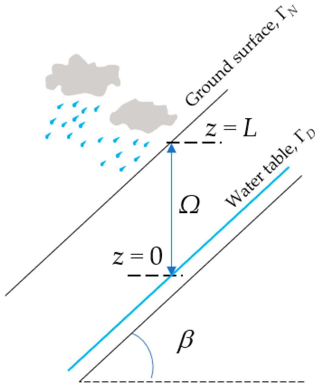
2.1. One-Dimensional Richards Equation

Let us denote by L the distance from the ground surface to the water table (Figure 1). We assume that there is no evaporation or water uptake by the roots. The governing equations for groundwater flow and corresponding boundary conditions are as follows:

$$\left\{\begin{array}{ll}{\displaystyle \frac{\partial \theta \left(z,t\right)}{\partial t}}={\displaystyle \frac{\partial }{\partial z}}\left[K\left(z,t\right){\displaystyle \frac{\partial \left(\phi \left(z,t\right)+z\right)}{\partial z}}\right],\hfill & z\in \mathrm{\Omega }\\ \theta \left(z,0\right)={\theta }_0\left(z\right),\hfill & z\in \mathrm{\Omega }\\ \theta \left(z,t\right)={\theta }_D\left(z,t\right),\hfill & z\in {\mathrm{\Gamma }}_D\\ n\cdot \left[K\left(z,t\right){\displaystyle \frac{\partial \left(\phi \left(z,t\right)+z\right)}{\partial z}}\right]=q_B\left(z,t\right),\hfill & z\in {\mathrm{\Gamma }}_N\end{array}\right.$$

(1)

where z and t represent coordinate [L] and time [T], respectively; K(z, t) is the unsaturated hydraulic conductivity [L/T]; φ(z, t) is the pore water pressure [L]; θ₀(z) is the initial water content [-]; θ_D(z) is the constant water content [-] at the Dirichlet boundary Γ_D, typically equal to saturated water content θ_s [-] at the water table; $n$ is the unit normal vector at the Neumann boundary Γ_N; and q_B(z, t) is the groundwater flux at the Neumann boundary [L/T], influenced by rainfall.

2.2. Analytical Solution of Effective Rainfall

In complex hydrogeological conditions, obtaining an analytical solution for Equation (1) is difficult. To derive an analytical solution, we make three assumptions: (i) The soil is homogeneous. (ii) The initial water content of the soil is a power function of position. (iii) Hydraulic conductivity, water content, and pore water pressure satisfy the following relationships [25]:

$$K\left(z,t\right)=K_s{e}^{\alpha \phi \left(z,t\right)}$$

(2)

$$\theta \left(z,t\right)={\theta }_r+{\displaystyle \frac{\left({\theta }_s-{\theta }_r\right)K\left(z,t\right)}{K_s}}$$

(3)

where K_s is the saturated hydraulic conductivity [L/T], and θ_r is the residual water content [-].

Performing several mathematical operations on Equation (3) provides the effective saturation of soil S_e [-], which is expressed as follows:

$$S_e\left(z,t\right)={\displaystyle \frac{\theta \left(z,t\right)-{\theta }_r}{{\theta }_s-{\theta }_r}}={\displaystyle \frac{K\left(z,t\right)}{K_s}}$$

(4)

We assume $z_{*}=\alpha z$, $L_{*}=\alpha L$, $q_{B*}=q_B/K_s$, and $t_{*}=\alpha K_{s}t/\left({\theta }_s-{\theta }_r\right)$. Equation (1) can be rewritten as follows:

$$\begin{array}{ll}{\displaystyle \frac{\partial S_e\left(z_{*},t_{*}\right)}{\partial t_{*}}}={\displaystyle \frac{{\partial }^2{S}_e\left(z_{*},t_{*}\right)}{{\partial z_{*}}^2}}+{\displaystyle \frac{\partial S_e\left(z_{*},t_{*}\right)}{\partial z_{*}}},& z_{*}\in {\mathrm{\Omega }}_{*}\\ S_e\left(z_{*},0\right)=e^{-z_{*}},\hfill & z_{*}\in {\mathrm{\Omega }}_{*}\hfill \\ S_e\left(0,t_{*}\right)=1,\hfill & z_{*}\in {\mathrm{\Gamma }}_{D*}\\ S_e\left(z_{*},t_{*}\right)+{\displaystyle \frac{\partial S_e\left(z_{*},t_{*}\right)}{\partial z_{*}}}=q_{B*},\hfill & z_{*}\in {\mathrm{\Gamma }}_{N*}\end{array}$$

(5)

Referring to Srivastava and Yeh [26], the analytical expression for S_e can be obtained with the aid of a Laplace transform, which is written as follows:

$$S_e\left(z_{*},t_{*}\right)=q_{B*}-\left(q_{B*}-1\right)e^{-z_{*}}-4q_{B*}{e}^{\left(L_{*}-z_{*}\right)/2}{\displaystyle \sum _{k=1}^{\infty }\frac{\sin \left({\lambda }_k{z}_{*}\right)\sin \left({\lambda }_k{L}_{*}\right)e^{-\left({\lambda }_k^2+\frac{1}{4}\right)t_{*}}}{1+L_{*}/2+2{\lambda }_k^2{L}_{*}}}$$

(6)

where λ_k is the positive root of the characteristic equation of $\tan \left(L_{*}x\right)+2x=0$. It should be noted that Equation (6) is not an explicit expression in terms of z, while the critical depths which are the boundaries distinguishing the saturated and unsaturated soils can be determined using the bisection method.

Based on the definition of the saturation of soil S_r [-], we obtain

$$S_r\left(z_{*},t_{*}\right)={\displaystyle \frac{{\theta }_r+\left({\theta }_s-{\theta }_r\right)S_e\left(z_{*},t_{*}\right)}{{\theta }_s}}$$

(7)

We employ the criterion of $S_r\ge 0.9$ mentioned in the Introduction to identify the saturated state of soil. The critical depths can be calculated by applying the bisection method to the following equation:

$$S_e\left(z_{*},t\right)={\displaystyle \frac{0.9{\theta }_s-{\theta }_r}{{\theta }_s-{\theta }_r}}$$

(8)

The differential equation for the volume of groundwater at position z (or $z_{*}$) from time 0 to t (or $t_{*}$) is

$$d{V}_w=\left(n-{\theta }_r\right)\left(S_e\left(z_{*},t\right)-S_e\left(z_{*},0\right)\right)dSd{z}_{*}=d{R}_e^{\ast }dS$$

(9)

Here, n is the soil porosity [-], dS is the differential area perpendicular to the z-direction [L²], and $d{R}_e^{*}$ is the differential of effective rainfall $R_e^{*}$ [L] at position z from time 0 to t.

Based on Equation (10), the effective rainfall accumulated in the soil column $z\in [a,b]\in \Omega$ from time 0 to t can be expressed as follows:

$$R_e^{*}\left(a,b,t\right)={\displaystyle \frac{n-{\theta }_r}{\alpha }}\left[{\displaystyle {\int }_{a_{*}}^{b_{*}}{S}_e\left(z^{\prime },t\right)d{z}_{*}}-{\displaystyle {\int }_{a_{*}}^{b_{*}}{S}_{e0}\left(z^{\prime }\right)d{z}_{*}}\right]$$

(10)

where ${\displaystyle {\int }_{a_{*}}^{b_{*}}{S}_{e0}d{z}_{*}=-\left(e^{-b_{*}}-e^{-a_{*}}\right)}$ and

$$\begin{array}{ll}{\displaystyle {\int }_{a_{*}}^{b_{*}}{S}_{e}d{z}_{*}}=& q_{B*}\left(b_{*}-a_{*}\right)+\left(q_{B*}-1\right)\left(e^{-b_{*}}-e^{-a_{*}}\right)\\ & +16q_{B*}{e}^{L_{*}/2}\left({\left.{\displaystyle \sum _{k=1}^{\infty }\frac{\left[\frac{1}{2}{e}^{-\frac{z_{*}}{2}}\sin \left({\lambda }_k{z}_{*}\right)+{\lambda }_k{e}^{-\frac{z_{*}}{2}}\cos \left({\lambda }_k{z}_{*}\right)\right]\sin \left({\lambda }_k{L}_{*}\right)e^{-\left({\lambda }_k^2+\frac{1}{4}\right)t_{*}}}{\left({\left[2{\lambda }_k\right]}^2+1\right)\left(1+L_{*}/2+2{\lambda }_k^2{L}_{*}\right)}}\right|}_{a_{*}}^{b_{*}}\right)\end{array}$$

Similar to Equation (10), the differential equation for the volume of groundwater from time t to the time of being fully saturated is as follows:

$$d{V}_w=\left(n-{\theta }_r\right)\left(1-S_e\right)dSdz=d{R}_{e}dS$$

(11)

where dR_e is the effective rainfall R_e [L] at position z from time t to the time of being fully saturated.

Based on Equation (12), the expression for R_e is as follows:

$$R_e\left(a,b,t\right)=n-{\theta }_r\left[b-a-{\displaystyle {\int }_a^b{S}_e\left(z^{\prime },t\right)dz}\right]={\displaystyle \frac{n-{\theta }_r}{\alpha }}\left[b_{*}-a_{*}-{\displaystyle {\int }_{a_{*}}^{b_{*}}{S}_e\left(z^{\prime },t\right)d{z}_{*}}\right]$$

(12)

The analytical expression for the total drainage volume Q_w(t) [L] at the water table at time t is as follows:

$$Q_w\left(t\right)=q_{B}t-R_e^{*}{\left(t\right)}_{a=0,b=L}$$

(13)

The derivative of Q_w(t) is the drainage rate q_w(t) at the boundary [L/T], which is written as follows:

$$q_w\left(t\right)=q_B+4q_B{\displaystyle \frac{n-{\theta }_r}{{\theta }_s-{\theta }_r}}{e}^{L_{*}/2}\left({\left.{\displaystyle \sum _{k=1}^{\infty }\frac{\left[\frac{1}{2}{e}^{-\frac{z_{*}}{2}}\sin \left({\lambda }_k{z}_{*}\right)+{\lambda }_k{e}^{-\frac{z_{*}}{2}}\cos \left({\lambda }_k{z}_{*}\right)\right]\sin \left({\lambda }_k{L}_{*}\right)e^{-\left(\frac{\alpha K_s\left[{\left(2{\lambda }_k\right)}^2+1\right]}{4\left({\theta }_s-{\theta }_r\right)}\right)t}}{\left(1+L_{*}/2+2{\lambda }_k^2{L}_{*}\right)}}\right|}_{a_{*}}^{b_{*}}\right)$$

(14)

To better quantify the proportion of effective rainfall to (total) rainfall, we define the index of effective rainfall for the soil at position z ($z\in [a,b]\in \Omega$) from time 0 to t as follows:

$$I_p^{*}\left(t\right)={\displaystyle \frac{R_e^{*}\left(a=0,b=L,t\right)}{P\left(t\right)}},\left(0\le I_p^{*}\le 1,0<P\left(t\right)\right)$$

(15)

where $P\left(t\right)=t{q}_B$ [L] represents the total rainfall. When $I_p^{*}=1$, $q_w\left(t\right)$ = 0. When $I_p^{*}=0$, $q_w\left(t\right)$ = q_B. Therefore, $1-I_p^{*}$ is defined as the rainfall loss index in a zone of interest.

2.3. Slope Stability with Effective Rainfall

2.3.1. Shear Strength of Unsaturated Soil

Fredlund et al. [27] proposed the extended Mohr–Coulomb criterion applicable to the shear strength τ [kPa] of unsaturated soil, which is written as follows:

$$\tau =c+\left(\sigma -u_a\right)\tan \varphi +\left(u_a-u_w\right)\tan {\varphi }_b$$

(16)

where c is the cohesion of soil [kPa], σ denotes the normal stress acting on the shear plane, u_a and u_w represent the normal air and water pressure, respectively, that are acting on the shear plane [kPa], and $\varphi$ and ${\varphi }_b$ are denoted as the internal friction angles [°] corresponding to the effective normal stress (σ − u_a) and matric suction (u_a − u_w), respectively.

Assuming that the effective stress generated by air is a constant throughout the soil, equal to a standard atmospheric pressure, $\left(u_a-u_w\right)=-\alpha {\gamma }_w\phi \left(z,t\right)$ and $-\alpha \phi \left(z,t\right)=\ln \left(\partial R_e^{*}\left(a=z,b=L,t\right)/\partial z\right)-\ln \left(n-{\theta }_r\right)$, the shear strength of unsaturated soil can be expressed as follows:

$$\begin{array}{ll}\tau \left(z,t\right)=& c+\left({\gamma }_s\left(L-z\right)+{\gamma }_w\left[R_e^{*}\left(a=z,b=L,t\right)-\left(n-{\theta }_r\right)\left(e^{-L}-e^{-z}\right)\right]\right)\cos \beta \tan \varphi \\ & +{\gamma }_w\ln \left({\displaystyle \frac{1}{n-{\theta }_r}}{\displaystyle \frac{\partial R_e^{*}\left(a=z,b=L,t\right)}{\partial z}}\right)\tan {\varphi }_b\end{array}$$

(17)

where γ_s and γ_w are the unit weights of soil particles and water [kN/m³], respectively, and $\beta$ is the slope [°]. According to Equation (18), the shear strength is a function of effective rainfall.

2.3.2. Shear Strength of Soil in the Transient Saturated Zone

When S_r at position z reaches 0.9, the soil is almost saturated. The shear strength can be described by the following equation:

$$\tau \left(z,t\right)=c+\left(\left({\gamma }_s\left(L-z\right)+{\gamma }_w\left[\begin{array}{l}{R}_e^{*}\left(a=z,b=L,t\right)\\ -\left(n-{\theta }_r\right)\left(e^{-L}-e^{-z}\right)\end{array}\right]\right)\cos \beta -{\gamma }_w{h}_w\left(z,t\right)\right)\tan \varphi$$

(18)

where h_w(z, t) is the depth of hydrostatic pressure at time t and position z.

Due to the assumptions we make, there are, theoretically, two transient saturated zones that are close to the ground surface and the water table, respectively. The h_w(z, t) in the transient saturated zone close to the ground surface, subjected to the two-stage linear assumption considered in Tang et al. [16], is expressed as follows:

$$h_w\left(z,t\right)=\left\{\begin{array}{cc}L-z,& L-\eta \left(L-z_1\left(t\right)\right)\le z<L\\ z-z_1\left(t\right),& z_1\left(t\right)<z<L-\lambda \left(L-z_1\left(t\right)\right)\end{array}\right.$$

(19)

where z₁ is the critical depth, which is the boundary distinguishing the transient saturated zone in the shallow saturated soil and unsaturated soil and can be determined relying on Equation (6), and $\eta$ is a constant with values within (0,1). The hydrostatic pressure in the transient saturated zone close to the water table is associated with the critical depth z₂, as determined by Equation (6). The corresponding expression is h_w(z,t) = z₂ (t) − z. When all the soil is saturated, we obtain z₁ = z₂, and h_w(z,t) = γ_w (L − z).

2.3.3. Slope Stability

The slope stability quantified and denoted as $F_s$ for an infinite slope is given as follows:

$$F_s=\left\{\begin{array}{c}{\displaystyle \frac{c+\left({\gamma }_s\left(L-z\right)+{\gamma }_w\left[R_e^{*}\left(a=z,b=L,t\right)-\left(n-{\theta }_r\right)\left(e^{-L}-e^{-z}\right)\right]\right)\cos \beta \tan \varphi +{\gamma }_w\ln \left(\frac{1}{n-{\theta }_r}\frac{\partial R_e^{*}\left(a=z,b=L,t\right)}{\partial z}\right)\tan {\varphi }_b}{\left({\gamma }_s{z}_s+{\gamma }_w{z}_w\right)\sin \beta }}\mathrm{unsaturated}\\ {\displaystyle \frac{c+\left(\left({\gamma }_s\left(L-z\right)+{\gamma }_w\left[\begin{array}{l}{R}_e^{*}\left(a=z,b=L,t\right)\\ -\left(n-{\theta }_r\right)\left(e^{-L}-e^{-z}\right)\end{array}\right]\right)\cos \beta -{\gamma }_w{h}_w\left(z,t\right)\right)\tan \varphi }{\left({\gamma }_s{z}_s+{\gamma }_w{z}_w\right)\sin \beta }}\mathrm{saturated}\end{array}\right.$$

(20)

Note that F_s is a piecewise function of effective rainfall which impacts the weight and matrix suction of soil. The numerator of the first line on the right-hand side of Equation (20) is the shear strength expressed by Equation (17), while that of the second line is the one described by Equation (18). The denominator in either the first line or the second is the sliding force, which is induced by the self-weight of both soil particles and groundwater.

2.4. Global Sensitivity Analysis

We employ three commonly used approaches to global sensitivity analyses to investigate the sensitivity of the slope stability to a variety of factors that may impact effective rainfall and, therefore, slope stability. The three methods are Sobol [28,29], Delta Test (DT) [30], and Random Sampling-High Dimensional Model Representation (RS-HDMR) [31]. The factors are denoted as X₁, X₂, …, X_m, where m is the number of factors of interest. The model output Y corresponds to the expression of Y = F(X) = F(X₁, X₂, …, X_m).

2.4.1. Sobol Method

The Sobol method uniquely decomposes the function F(X) into a sum of its components:

$$F(X)=F_0+{\displaystyle \sum _{i=1}^m{F}_i(X_i)+{\displaystyle \sum _{1\le i<j\le m}{F}_{ij}(X_i,X_j)}}+\dots +F_1,\dots ,m(X_1,X_2,\dots ,X_m)$$

(21)

where F₀ is a constant representing the mean of F(X), F_i(X_i) is the first-order component function, and F_ij(X_i, X_j) represents the coupling effect of X_i and X_j on Y, with higher-order terms following similarly.

The variance of F(X) can be expressed as the sum of variances of these decomposition terms:

$$V={\displaystyle \sum _{i=1}^m{V}_i+{\displaystyle \sum _{1\le i<j\le m}{V}_{ij}}+\dots +V_{1,2,\dots ,m}}$$

(22)

where V(·) is the variance operator, and f_X(x) denotes the joint probability density function of the input variable. The variance of F(X) can be decomposed into contributions from the variance of each factor and the variance of interactions between factors, as follows:

$$V_{i,j,\dots ,m}=Var[F_{i,j,\dots ,m}(X_i,X_j,\dots ,X_m)]={\displaystyle \int F_{i,j,\dots ,m}^2}(X_i,X_j,\dots ,X_m){\displaystyle \prod _{j\ne i,\dots ,m}^m[f_{X_j}(x_j)d{x}_j]}$$

(23)

$$V=Var(Y)={\displaystyle \int F^2(X)f_X(x)dx-F_0^2}$$

(24)

The main effect index of X_i, $R_i$, which corresponds to the first-order effect of X_i on Y is given as follows:

$$R_i=V_i/V$$

(25)

The total sensitivity index $R_{Ti}$, which quantifies both the impacts of the variability of X_i and its interactions with other factors on the variance of the output response, is expressed as follows:

$$R_{Ti}=1-R_{~i}$$

(26)

where $R_{~i}$ is the ratio of the sum of all variance components to the total variance without X_i, i.e., $R_{~i}=V_{~i}/V$,$V_{~i}=Var[E(Y|X_{~i})]$.

2.4.2. DT Method

In the DT method, the cumulative effect of the uncertain factor of X_i on the probability density (or probability distribution) of Y is denoted as $s(X_i)$, which is expressed as

$$s(X_i)={\displaystyle \int \left|f_Y(y)-f_{Y\left|X_i\right.}(y)\right|dy}$$

(27)

where $f_Y(y)$ and $f_{Y\left|X_i\right.}(y)$ are the unconditional probability density function and conditional probability density function of Y, respectively.

Therefore, the formula for calculating the expected value of $s(X_i)$ is as follows:

$$E_{X_i}[s(X_i)]={\displaystyle \int f_{X_i}(x_i)[{\displaystyle \int \left|f_Y(y)-f_{Y\left|X_i\right.}(y)\right|dy}]}d{x}_i$$

(28)

The impact of the variable X_i on the model output Y can be quantified by the moment-independent importance measure δ_i,

$${\delta }_i={\displaystyle \frac{1}{2}}{E}_{X_i}[s(X_i)]$$

(29)

The bootstrap technique is employed to adjust the moment-independent indicators. The revised calculation formula for $\widehat{\widehat{\delta }}$ is

$$\widehat{\widehat{\delta }}=\widehat{\delta }-\widehat{bias(\widehat{\delta })}=2\widehat{\delta }-{\overline{\delta }}^{*}$$

(30)

where $\widehat{bias(\widehat{\delta })}={\overline{\delta }}^{*}-\widehat{\delta }$, $\widehat{\widehat{\delta }}$ and $\stackrel{⌢}{\delta }$ are consistent estimators of δ, and ${\overline{\delta }}^{*}$ is the moment-independent importance measure adjusted through Bootstrap techniques.

2.4.3. RS-HDMR Method

The High Dimensional Model Representation (HDMR) method characterizes the relationship between X and Y in a similar way to Equation (22). The RS-HDMR is proposed relying on the HDMR algorithm and applying random sampling within the feasible domain of the randomly selected N sample points. It uses orthogonal basis functions to determine its component functions. The expression of F(X) is given by the equation:

$$F(X)=F_0+{\displaystyle \sum _{i=1}^m{\displaystyle \sum _{r=1}^k{\alpha }_r^i{B}_r(X_i)}}+{\displaystyle \sum _{i<j}{\displaystyle \sum _{\mathrm{w}=1}^l{\displaystyle \sum _{\mathrm{z}=1}^o{\beta }_{\mathrm{wz}}^{ij}{B}_{\mathrm{w}}(X_i)}}}{B}_{\mathrm{z}}(X_j)$$

(31)

where k, l, and o are integer constants, which represent the order of orthogonal polynomials. ${\alpha }_r^i$ and ${\beta }_{\mathrm{wz}}^{ij}$ are constants to be determined, which can be obtained through least squares regression. B_r(X_i), B_w(X_i) and B_z(X_j) are orthogonal basis functions determined in terms of the sample set.

The variance of each term in the RS-HDMR expansion can be expressed as follows:

$$V_i={\displaystyle \sum _{r=1}^k{({\alpha }_r^i)}^2},V_{ij}={\displaystyle \sum _{\mathrm{w}=1}^l{\displaystyle \sum _{\mathrm{z}=1}^m{({\beta }_{\mathrm{wz}}^{ij})}^2}}$$

(32)

The total variance of Y can be expressed as follows:

$$V={\displaystyle \frac{1}{n}}{\displaystyle \sum _{i=1}^n{F}^2(X_{\mathrm{i}})-F_0^2}$$

(33)

The RS-HDMR method obtains first- and second-order sensitivity indexes, S_i and S_ij, as V_i and V_ij normalized by V.

The Sobol method relies on the global distribution of Y and decomposes the global variance of Y into components corresponding to individual factors. The Sobol method cannot tell the differences between response surfaces with identical variances but different structures and/or derivative distributions. Additionally, the Sobol method does not quantify sensitivity relying on the high-order statistical moments (i.e., skewness and kurtosis) of Y, due to its variance-based nature. The DT method does not account for interactions between factors. The latter are significant in many environmental systems. The RS-HDMR method yields global sensitivities, since it relies on decomposing the model function over the entire space of factors. The convergence of sensitivity provided through the RS-HDMR method depends on the smoothness of the model function. To combine the advantages while minimizing the disadvantages of different methods, we compute the sensitivity of slope stability to each factor by using the indexes R_Ti(X), $\widehat{\widehat{\delta }}$, and S_i, corresponding to the three respective methods mentioned above. An arithmetic average of the three indexes is used to comprehensively evaluate the sensitivity.

3. Illustrative Examples

We consider exemplary cases in which the mechanical properties of the soil correspond to a granite residual soil [27,32] and the hydrogeological conditions (including rainfall intensity and the thickness of unsaturated zone) correspond to southeastern China. The parameters for the cases are listed in

Table 1. Parameters based on a granite residual soil [2,27,32,33,34,35] used for the analytical and numerical solutions.

Parameter	Value	Unit
c	28.9	kPa
ϕ	33.4	°
ϕb	15.3	°
β	30	°
γs	24.89	kN/m3
Ks	1.29 × 10−5	m/d
qB*	0.1, 0.5, 1.0	mm/d
α	0.32, 1.28, 5.12	L/m
L	2, 3, 8	m
θs	0.45	-
θr	0.05	-

. Note that we consider three values each of q_B*, α, and L to explore temporally how the rainfall intensity, the air-entry value of soil (i.e., the reciprocal of α), and the thickness of the unsaturated zone influence the hydraulic dynamics and shear strength. To verify the reliability of the analytical solutions derived in this study, the accuracies of the analytical solutions of S_e, S_r, φ, θ, and q_w are compared against their corresponding numerical solutions when considering q_B*, α, and L equal to 0.5 mm/d, 1.28 L/m, and 3 m, respectively. In the remaining text, the values of q_B*, α, and L are set to these three respective values, unless specified otherwise. In the numerical solutions, a standard finite element approach is employed to discretize Equations (1)–(3). A one-dimensional mesh associated with 100 elements of the same size is considered. The total simulation time is 2 × 10⁵ s (approximately 27.78 h). A fixed time step of 100s is considered in the numerical model. The number of positive roots of ${\lambda }_k$ for all characteristic equations used in the analytical solutions is 1000.

The factors and their corresponding uncertainties for performing global sensitivity analyses are listed in

Table 2. Factors and their uncertainties considered in global sensitivity analysis.

Factor	Distribution	Shape Parameters for PDF		Unit	References
c	lognormal	υ, σ	25.000, 3.333	kPa	[36]
ϕ			25.000, 1.667	°	[2]
β			40.000, 3.333	°	[37,38]
γs			19.000, 0.333	kN/m3	[39,40]
Ks			1.296, 0.215	m/d	[37,41]
α	uniform	${\Gamma }_l$, ${\Gamma }_u$	0.320, 5.120	L/m	[42]
L			0.500, 8.000	m	[37,43]

. The probability density functions (PDF) for c, ϕ, β, γ_s, and K_s are considered as lognormal, with an expression of $f(x)={\displaystyle \frac{1}{qx\sqrt{2\pi }}}\exp [-\frac{{(\ln x-p)}^2}{2q^2}]$, where p and q are the mean and the standard deviation, respectively, of the lognormal distribution. In this context, the mean $\upsilon$ and the standard deviation $\delta$ corresponding a normal distribution are written as $\upsilon =\exp (p+0.5q^2)$ and $\delta =\sqrt{[\exp (q^2)-1]\exp (2p+q^2)}$, respectively. The parameters α and L are associated with uniform distributions, with upper and lower limits denoted as ${\Gamma }_l$ and ${\Gamma }_u$, respectively. We aim to investigate the sensitivity of slope stability to its main influencing factors under heavy rainfall. Therefore, we set q_B equal to K_s. The sensitivity indexes are evaluated with the sample size N = 500, 1000, 2000, 3000, 4000, 5000, 7500, and 10,000.

4. Results and Discussion

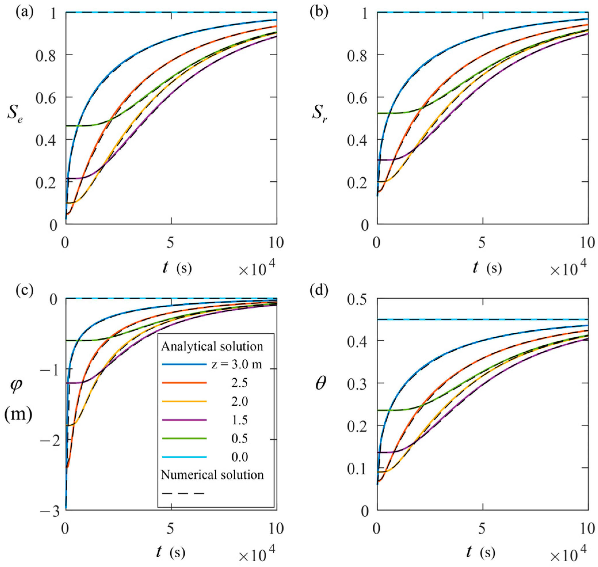
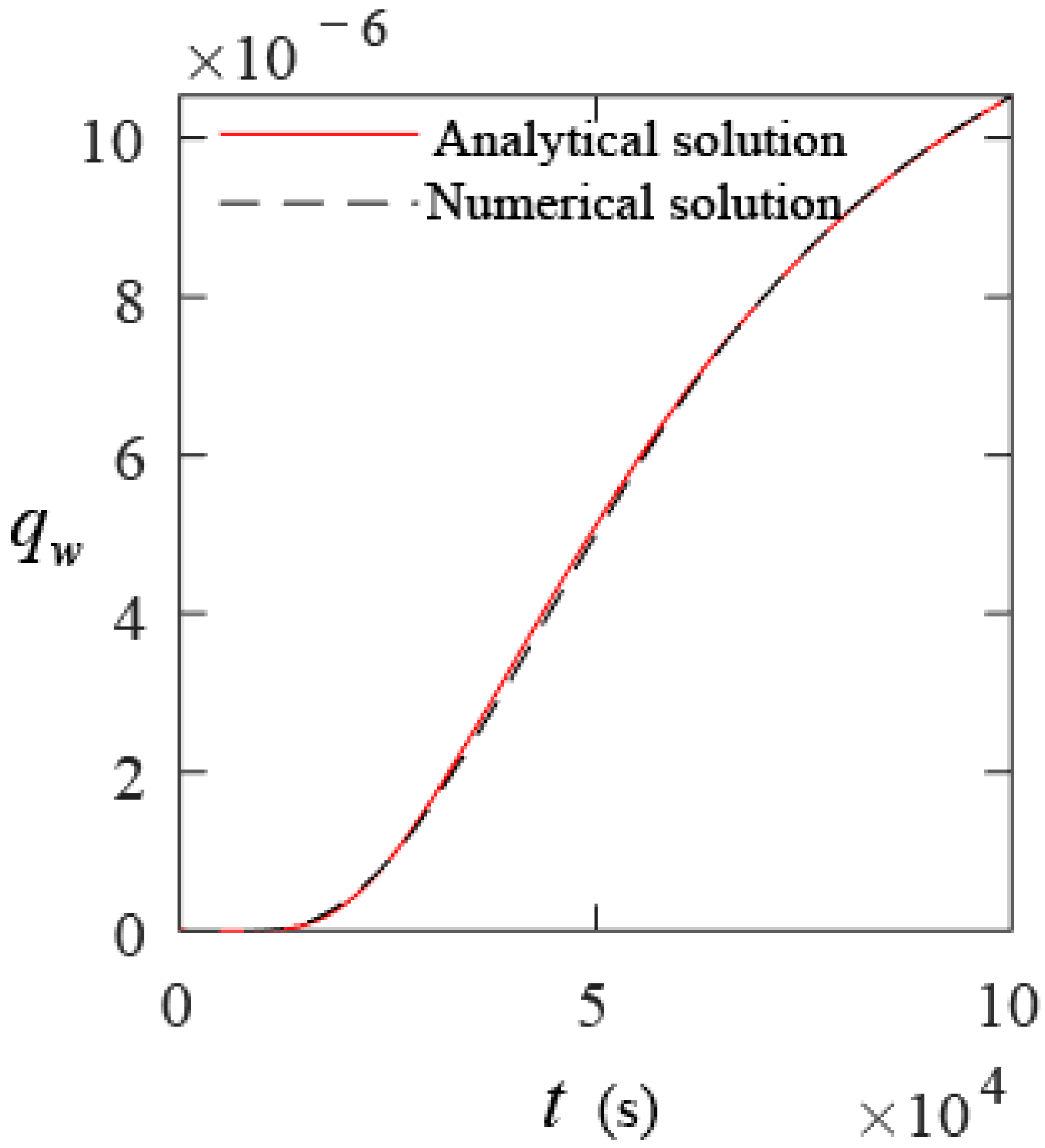
4.1. Analytical and Numerical Solutions

Figure 2 shows the temporal evolution of S_e (Figure 2a), S_r (Figure 2b), φ (Figure 2c), and θ (Figure 2d) obtained through the analytical and standard finite element techniques at different depths of soil (z = 0.0, 0.5, …, 3.0 m). The analytical solutions (colored solid lines) are visually consistent with their corresponding numerical solutions (black dashed lines). Considering the analytical solutions as references, the maximum relative differences between the analytical and numerical solutions for S_e, S_r, φ, and θ are 0.29%, 0.26%, 0.00%, and 0.26%, respectively. These results indicate that the analytical solutions for S_e, S_r, φ, and θ are accurate and reliable.

Figure 3 depicts the temporal evolution of q_w obtained through the analytical and numerical techniques. The analytical solutions (red solid line) are visually consistent with their corresponding numerical solutions (black dashed line). Using the analytical solutions as a reference, the relative difference between the analytical and the numerical solutions ranges from 0.53% to 1003%. The high relative differences correspond to the position where q_w is close to zero at the early stage of the rainfall. Most of the relative differences are less than 5.00%. These results indicate that the analytical solutions for q_w are accurate and reliable, which at least partially suggests that the analytical solutions of effective rainfall are reliable since Q_w, and therefore q_w, are functions of effective rainfall.

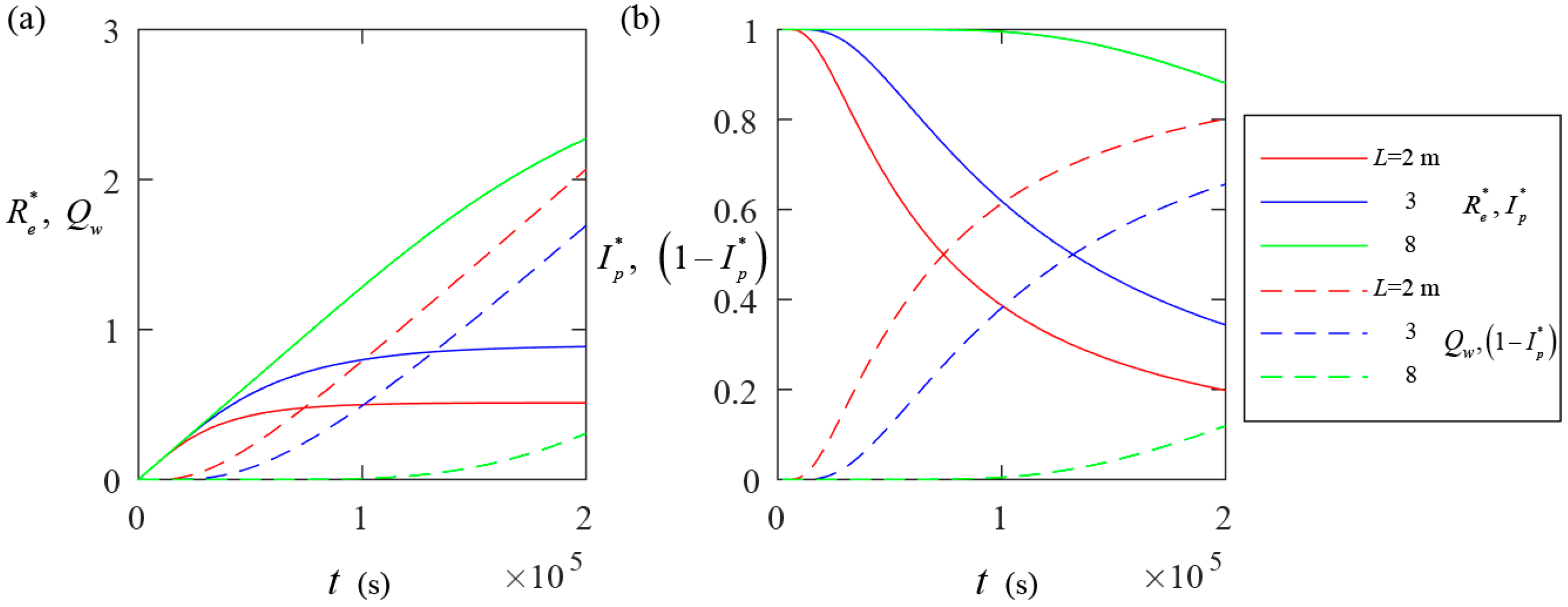
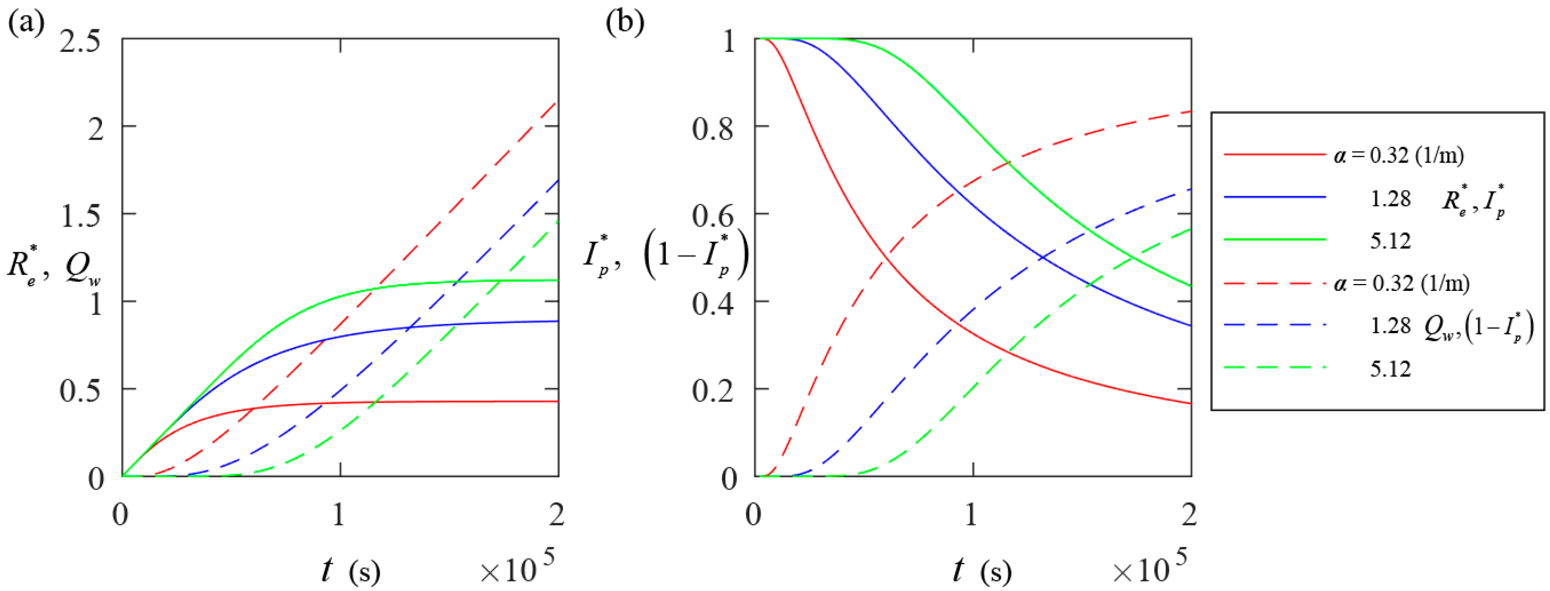
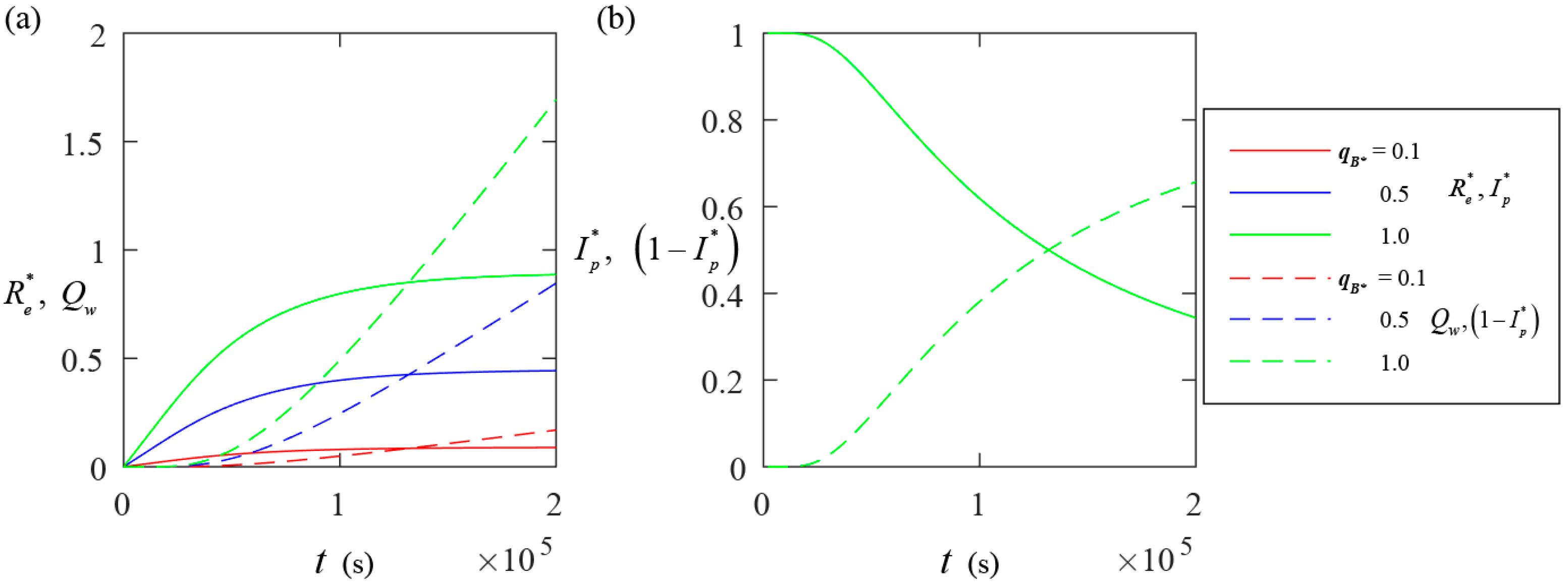
4.2. Temporal Evolution of Effective Rainfall

We consider L is equal to 2, 3, and 8 m, while the other parameters in Table 1 remain the same as in Section 4.1. Figure 4a shows the temporal evolution of the values of $R_e^{*}$ at the water table (a = 0 and b = L in Equation (11)) and Q_w. As shown in Figure 4a, when L = 2, $R_e^{*}$ increases with time until reaching a constraint value, while Q_w continues to rise. As L increases, the values of $R_e^{*}$ increase, while the values of Q_w decrease. Figure 4b displays the temporal evolution of the values of $I_p^{*}$ and 1 − $I_p^{*}$ corresponding to the results in Figure 4a. As L increases, the changing velocity of $I_p^{*}$ gradually slows down with time, which is related to the fact that $R_e^{*}$ increases as the thickness of the unsaturated zone increases. These results are linked to the fact that the unsaturated zone located at the slope toe needs less time to reach saturation compared with the slope top because the former is associated with a thinner unsaturated zone than the latter.

We consider α equal to 0.32, 1.28, and 5.12, while the other parameters remain the same as in Section 4.1. Figure 5a shows the temporal evolution of the values of $R_e^{*}$ and Q_w. It can be seen from Figure 5a that effective rainfall increases as α increases, while a reversing trend is observed for Q_w. Figure 5b presents the temporal evolution of the values of $I_p^{*}$ and 1 − $I_p^{*}$ corresponding to the results in Figure 5a. As shown in Figure 4, large values of $I_p^{*}$ and 1 − $I_p^{*}$ correspond to large values of $R_e^{*}$ and Q_w. An explanation for these results is that a large value of α causes the effective soil saturation to be more sensitive to the pore water pressure. This results in more rainfall being retained in the unsaturated zone under the same infiltration recharge when α is larger, leading to higher values of the effective rainfall index.

We consider $q_{B^{*}}$ equal to 0.1, 0.5, and 1.0, while the other parameters remain the same as in Section 4.1. Figure 6 shows the temporal evolution of the values of $R_e^{*}$ and Q_w (Figure 6a) and the corresponding values of $I_p^{*}$ and 1 − $I_p^{*}$ (Figure 6b). As $q_{B^{*}}$ increases, the values of $R_e^{*}$ and Q_w generally increase. This is different from the results in Figure 4a and Figure 5a, as an increased value of $q_{B^{*}}$ indicates intensifying infiltration recharge, which leads to simultaneous increases in both effective rainfall and discharge. There is only one green solid (or dashed) curve for $I_p^{*}$ (or 1 − $I_p^{*}$) shown in Figure 6b. The reason is that $I_p^{*}$ is independent of $q_{B^{*}}$, which can be inferred from Equation (16).

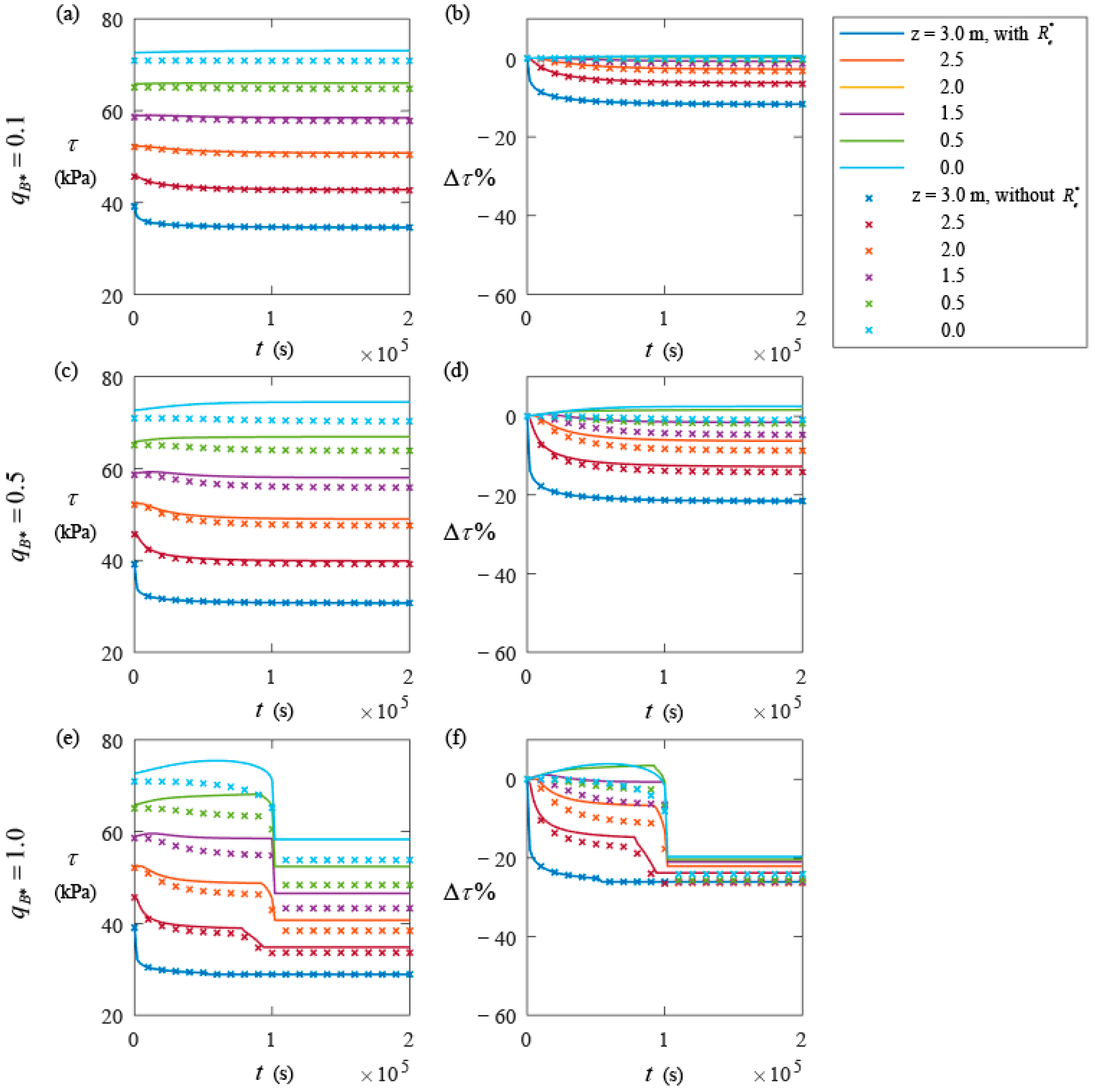
4.3. Spatiotemporal Distribution of Shear Strength

Similar to Figure 5, we consider α equal to 0.32, 1.28, and 5.12 L/m, while keeping the other parameters the same as in Section 4.1. Figure 7 shows the temporal evolution of the values of τ and their percentage change ($\Delta \tau \%$) with reference to that at the initial time when α = 0.32 (L/m, Figure 7a,b), 1.28 (L/m, Figure 7c,d), and 5.12 (L/m, Figure 7e,f). The solid and dashed lines in Figure 7 indicate the results with and without effective rainfall, respectively. When considering effective rainfall, the shear strength of soil generally increases with soil depth as the self-weight of the soil increases. This phenomenon disappears when effective rainfall is ignored. As α increases, $R_e^{*}$ increases, and the values of τ overall decrease more in the sense of that $\Delta \tau \%$ overall decrease at the end of the simulation time. This is related to the behavior of $R_e^{*}$ in Figure 5. The increase in $R_e^{*}$ leads to an increase in pore water pressure, which results in the overall decrease in the shear strength. Different values of α lead to various spatiotemporal distributions of effective rainfall (see Figure 5), influencing the percentage decrease in the shear strength at different soil depths. For example, when α = 0.32 L/m, the curve with the overall smallest $\Delta \tau \%$ corresponds to z = 0.5 m, whereas for α = 1.28 and 5.12 L/m, the curves with the overall smallest $\Delta \tau \%$ correspond to z = 3.0 and 2.5 m. The value of α is the reciprocal of the air-entry value of the soil. As α increases, the air-entry value of the soil decreases, improving the sensitivity of the unsaturated hydraulic conductivity to the pore water pressure. Additionally, α is typically physically correlated with the permeability of soil. For example, the α for sandy soil, silt, and clay are approximately in the ranges of [1.57, 7.84], [0.14, 1.4], and [0.02, 0.20] (L/m), respectively. As the value of α increases, the permeability of the soil increases, leading to quick responses in the hydraulic dynamics of groundwater in the unsaturated zone. Additionally, it is worth noting that the difference in the shear strength of soil with and without effective rainfall increases with the depth of the soil. This is because the effect of effective rainfall on the slope stability increases with depth.

Except for $q_{B^{*}}$, the other parameters remain the same as in Section 4.1. Figure 8 presents the temporal evolution of the values of τ and $\Delta \tau \%$ for $q_{B^{*}}$ = 0.1 (Figure 8a,b), 0.5 (Figure 8c,d), and 1.0 (Figure 8e,f). The solid and dashed lines in Figure 8 indicate the results with and without effective rainfall, respectively. As the rainfall intensity increases, $R_e^{*}$ increases (see Figure 6a), leading to different behavior of τ at various soil depths. When $q_{B^{*}}$ = 0.1, the values of τ of the shallow soil approaching the ground surface show descending trends, while the values of τ of the deep soil show ascending trends. This is because the pore water pressure of the deep soil has not yet been significantly affected by the infiltration recharge at the early stage of rainfall, while the increase in the self-weight of the soil caused by the infiltration recharge leads to an increase in the shear strength. When $q_{B^{*}}$ = 1, the descending and ascending speeds of τ become higher with reference to $q_{B^{*}}$ = 0.1.

An interesting phenomenon is that the temporal evolution of τ exhibits staged descending/ascending trends. A joint analysis of Figure 7 and Figure 8 together with Equations (19) and (20) reveals that this phenomenon is consistent with the theories in Section 2. The temporal evolution of the shear strength of soil can be divided into four periods: (a) strength improvement due to the increasing self-weight of soil caused by rainfall infiltration, (b) strength reduction controlled by the increasing pore water pressure, (c) strength reduction due to the effect of hydrostatic pressure in the transient saturation zone, and (d) stable strength when all the soil is fully saturated. Concerning (a), infiltration increases effective rainfall and, therefore, the self-weight of soil close to the ground surface, which enhances effective normal stress (in Equation (18)) of the deep soil. As infiltration proceeds, the increase in pore water content reduces matrix suction and then the shear strength. Concerning (c), once the transient saturated zone appears, its hydrostatic pressure leads to a quick drop in shear strength as well. The temporal variation in the shear strength becomes minor since the soil is almost saturated. Note that not all the shear strength of soil at any depth is associated with these four periods. For example, the shallow soil approaching the ground surface corresponds to a very short (or even neglectable) period of (a), since infiltration quickly occurs. Conversely, the deep soil has a relatively long period of (a). When effective rainfall is not taken into account, the period of (a) disappears and the shear strength is underestimated. With effective rainfall, the increase in self-weight can be quantified, enhancing the shear strength by the increased water pressure acting on the shear plane. The magnitude of underestimated shear strength increases with the depth of soil, since the water pressure acting on the shear plane increases.

The quick drop in shear strength is caused by the instantaneous function of hydrostatic pressure existing in the transient saturated zone. The hydrostatic pressure distribution in the transient saturated zone is complicated. Several experimental results indicate that the hydrostatic pressure in the transient saturated zone exhibits complex non-linearity [44]. Tang et al. [16] assumes the hydrostatic pressure distribution can be characterized by a piecewise function. Although the validity of the assumption has not been verified, it is consistent with the physical mechanism where the pore water pressure (or hydrostatic pressure) at the boundaries between the transient saturated zone and the unsaturated soil is zero. Additionally, when the air-entry value of soil is low, the effective rainfall for the shallow soil increases rapidly with rainfall. This leads to a quicker decrease in the shear strength, making the slope more prone to shallow shear failure.

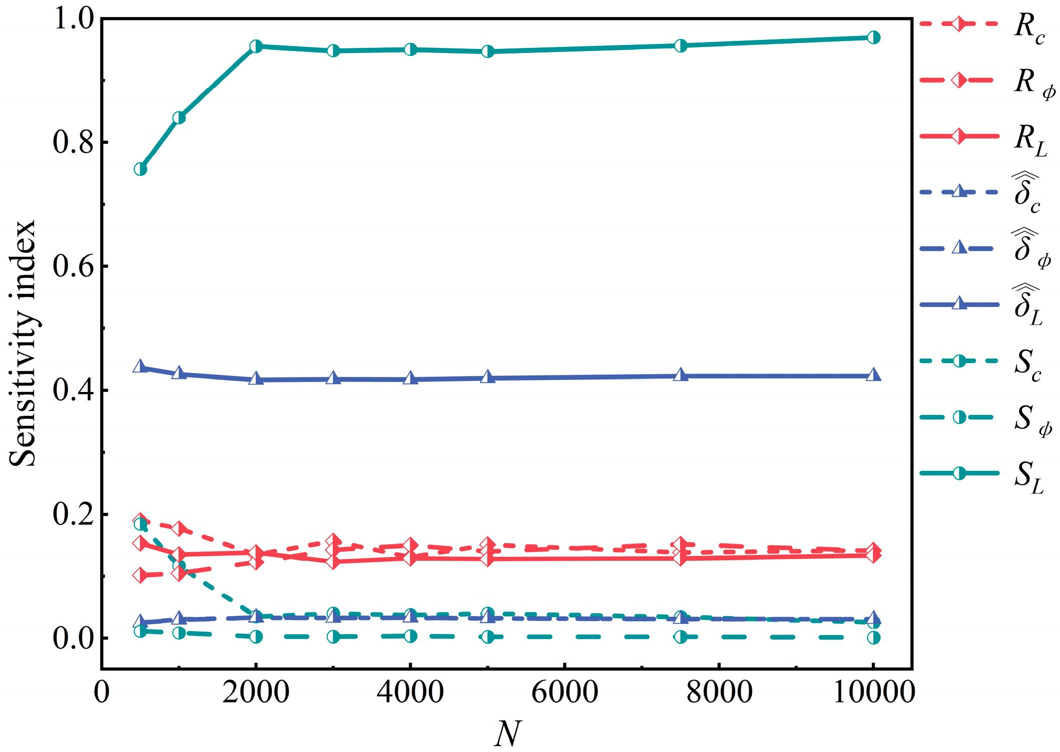
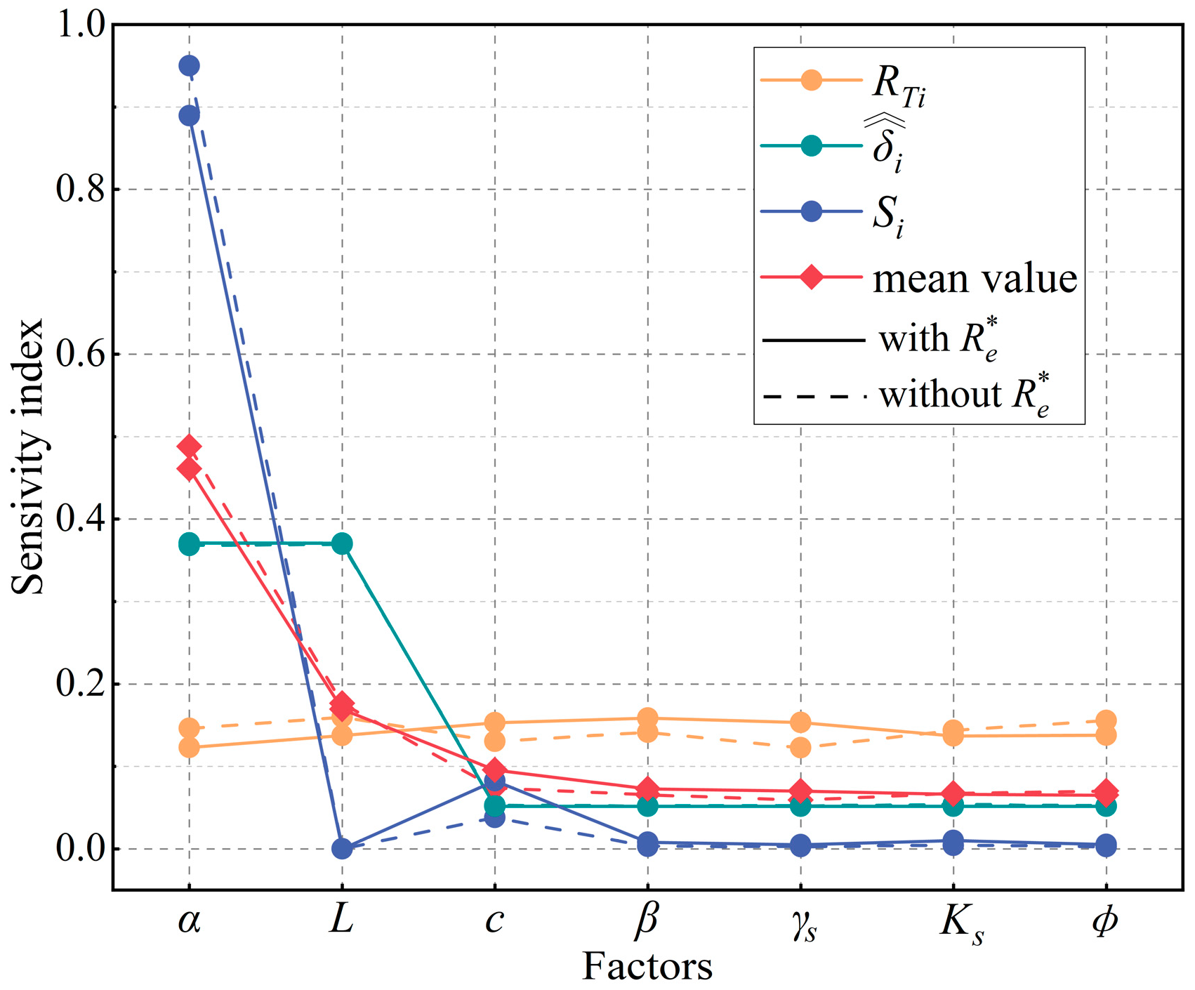
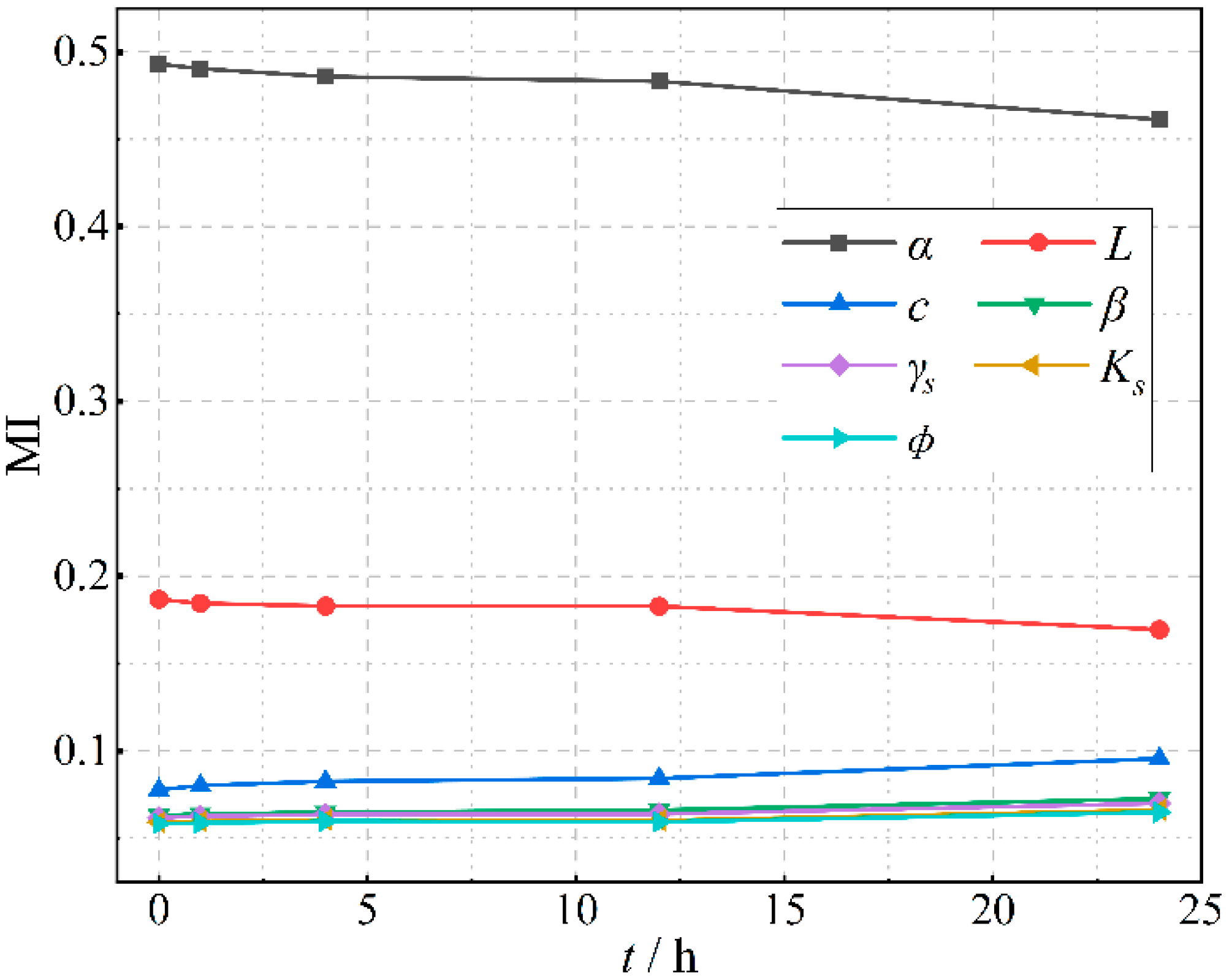
4.4. Sensitivity of Slope Stability

Figure 9 depicts the values of R_Ti, $\widehat{\widehat{\delta }}$_i, and S_i (with i = c, ϕ, and L) varying with N when t = 0. To better show the variations in the indexes with limited space, we only present the indexes for c, ϕ, and L. The values oscillate when N is small, but generally stabilize when N ≥ 5000. Specifically, the sensitivity index values at N = 5000 are almost equal to their counterparts at N = 7500, with an absolute difference of less than 0.01. Considering the values at N = 5000 as references, the relative differences between the values at N = 5000 and 7500 range from 1.26% to 8.35%. As such, we adopt N = 5000 in the remaining analyses.

Figure 10a shows the temporal behaviors of F_s when considering the first 100 realizations (gray lines) of factors and the corresponding mean of F_s (red line). Figure 10b plots the corresponding relative differences of F_s (${\Delta }_{F_s}$, gray lines) with and without effective rainfall and the mean of the relative differences (red line). The slope stability generally decreases with time, under the effect of rainfall. Since the factors are associated with uncertainty, the temporal values of F_s vary across the different realizations. The temporal values of ${\Delta }_{F_s}$ generally increase with time. The max value of ${\Delta }_{F_s}$ in Figure 10b is 8.34%. These results indicate the significance of considering effective rainfall as time evolves.

Figure 11 displays the R_Ti, $\widehat{\widehat{\delta }}$_i, and S_i (with i = c, ϕ, β, γ, K_s, α, and L) indexes for different factors when t = 24 h and N = 5000. The solid and dashed lines indicate the results with and without effective rainfall, respectively. With effective rainfall, the factor associated with the highest sensitivities obtained through the Sobol method was β, followed by c and then γ, while the factor associated with the lowest sensitivity was K_s. Without effective rainfall, the factor associated with the highest sensitivities obtained through the Sobol method was ϕ, followed by L. Either with or without effective rainfall, the factor associated with the highest sensitivities obtained through the DT method was L, followed by α, while the factor associated with the lowest sensitivity was c. Note that the sensitivity indexes for individual factors obtained with or without effective rainfall are close to each other and visually indistinguishable. Either with or without effective rainfall, the factor associated with the highest sensitivities obtained through the RS-HDMR method was α, followed by c, while the factor associated with the lowest sensitivity was L. These results show that α is the factor associated with the highest sensitivity, either through the DT or RS-HDMR method, which is consistent with the fact that when rainfall is sufficient, the hydraulic dynamic in the slope is significantly impacted by the air-entry value of soil. The factors β, γ_s, K_s, and ϕ are consistently associated with the lowest sensitivities through both the DT and RS-HDMR methods.

As introduced in Section 2.4, different methods are associated with different theoretical backgrounds, and therefore, produce various sensitivities. We compute the arithmetic mean of the three indexes (denoted as MI) for each factor to comprehensively assess the sensitivities of the slope stability to the factors. The sensitivity order in terms of MI is α > L > c > β > γ_s > K_s > ϕ. According to the ranking results, the thickness of the unsaturated zone and the parameter of the reciprocal of the air-entry value of soil are the main sensitive factors. Effective rainfall is a function of L and α. L and α can jointly reflect the hydrological response of groundwater under effective rainfall. The result that the sensitivity of c is higher than ϕ is consistent with the findings provided by [45,46]. Lin et al. [47] report the order of the sensitivity of slope stability to various factors as c > the height of slope (H_L) > ϕ > β > the pore water pressure coefficient (μ) > γ_s. Furthermore, the order provided by Lei et al. [48] is β > c > μ > H_L > γ_s > ϕ. These studies were performed under natural conditions, and the effect of rainfall on the slope stability was not taken into account. In this study, we consider this effect and obtain an order of sensitivity somewhat different from that of previous studies. Particularly, the sensitivities of the factors concerning rainfall infiltration become significant. This result suggests the need to identify the soil types associated with different soil water characteristic curves when performing landslide prediction and prevention. The sensitivity related to K_s is not as high as L and α. This is because when performing global sensitivity analyses, we set q_B equal to K_s to mimic a scenario of heavy rainfall. We note that this consideration is somewhat inconsistent with a practical engineering system where rainfall infiltration varies spatiotemporally within the slope. More complicated conditions should be studied in future work.

Figure 12 shows the temporal evolution of MI for each factor when N = 5000. The factors associated with the highest sensitivities in terms of MI was α, followed by L. The values of MI for both α and L decrease as time increases, while those for c and other factors generally increase with time increases. The air-entry value of soil has an important impact on the hydraulic dynamics in the unsaturated zone. Additionally, it is visually hard to tell the most sensitive one among the remaining factors.

5. Conclusions

We derive the analytical expressions of effective rainfall $R_e^{*}$, the shear strength of soil τ, and the slope stability F_s when considering a scenario of infinite slope and when groundwater flow is conceived as the one-dimensional Richards equation. Numerical solutions are used as references to partially verify the accuracy of the analytical solution. The granite residual soil in southeastern China is considered as an exemplar when performing numerical and analytical simulations. Various combinations of the reciprocal of the air-entry value of soil α, infiltration intensity q_B, and the thickness of the unsaturated zone L are considered to locally and visually check how these factors influence effective rainfall and the shear strength of soil. Additionally, the arithmetic average of three sensitivity indexes obtained through three approaches to global sensitivity analysis, respectively, are used to quantify the sensitivity of the slope stability to a variety of factors. The main conclusions drawn from the results are summarized as follows.

The analytical solutions of the effective saturation of soil S_e, the saturation of soil S_r, the pore water pressure φ, the water content θ, and the drainage rate q_w at the bottom boundary are verified to be correct, in the sense that the relative differences between the analytical solutions and their numerical counterparts are mostly less than 5%.

The shear strength of soil and the slope stability are functions of effective rainfall. Under the influence of effective rainfall, the temporal evolution of τ can be generally divided into four periods: (a) strength improvement due to the increase in the self-weight of soil caused by rainfall infiltration, (b) strength reduction controlled by the increase in the pore water pressure, (c) strength reduction due to the effect of hydrostatic pressure in the transient saturation zone, and (d) stable strength when all the soil is fully saturated.

The air-entry value of soil (i.e., the reciprocal of α) reflects the soil water characteristics and helps to understand the mode and mechanism of slope failure. Large values of α corresponding to large effective rainfall lead to a rapid decrease in the shear strength of the shallow soil due to rainfall infiltration, which increases the probability of the shear failure of the slope.

The results of the global sensitivity analyses reveal that the sensitivity order in terms of MI is α > L > c > β > γ_s > K_s > ϕ, where c is the cohesion of soil, β is the slope angle, γ_s is the unit weights of soil particles, K_s is the saturated hydraulic conductivity, and $\varphi$ is the internal friction angle. It is interesting to note that the first two leading factors are inputs for computing effective rainfall, which at least suggests that effective rainfall has important impacts on slope stability.

Avenues for future developments include theoretical analyses and corresponding synthetic studies related to scenarios associated with seismic load, heterogeneous conductivity, and transient intensity of rainfall. Field-scale studies, which can cope with spatiotemporal rainfall and landslides, will then constitute an important future research direction. The appropriate design of these kinds of studies would require broad participation to markedly advance knowledge across the entire subsurface hydrology and engineering geology research field.

References

1. Rabie, M. Comparison study between traditional and finite element methods for slopes under heavy rainfall. HBRC J. 2014, 10, 160–168. [Google Scholar] [CrossRef]
2. Jian, W.B.; Hu, H.R.; Luo, Y.H.; Tang, W.Y. Experimental study on deterioration of granitic residual soil strength in wetting-drying cycles. J. Eng. Geol. 2017, 25, 592–597. [Google Scholar] [CrossRef]
3. Zeng, L.; Shi, Z.N.; Fu, H.Y.; Bian, H.B. Influence of rainfall infiltration on distribution characteristics of slope transient saturated zone. China J. Highw. Transp. 2017, 30, 25–34. [Google Scholar] [CrossRef]
4. Qiu, X.; Jiang, H.B.; Ou, J.; Liu, Z.W.; Chen, M. Stability analysis method of “transient” saturated-unsaturated slope. China J. Highw. Transp. 2020, 33, 63–75. [Google Scholar] [CrossRef]
5. Peiffer, L.; Inguaggiato, C.; Wurl, J.; Fletcher, J.M.; Martínez, M.G.O.; Martínez, D.C.; Legrand, D.; Morales, P.H.; Reinoza, C.E.; Tchamabé, B.C.; et al. Geochemistry of coastal geothermal systems from southern Baja California peninsula (Mexico): Fluid origins, water-rock interaction and tectonics. Chem. Geol. 2024, 670, 122316. [Google Scholar] [CrossRef]
6. Shu, B.; Chen, J.J.; Xue, H. Experimental study of the change of pore structure and strength of granite after fluid-rock interaction in CO2-EGS. Renew. Energy 2024, 220, 119635. [Google Scholar] [CrossRef]
7. Abd, A.I.; Fattah, Y.M.; Mekkiyah, H. Relationship between the Matric Suction and the Shear Strength in Unsaturated Soil. Case Stud. Constr. Mater. 2020, 13, e00441. [Google Scholar] [CrossRef]
8. Antonello, T.; Luigi, P.; Enrico, C. Rainfall Threshold for Shallow Landslide Triggering Due to Rising Water Table. Water 2022, 14, 2966. [Google Scholar] [CrossRef]
9. Duc, B.T.; Ha, N.D.; Kim, N.T.; Hong, L.L.; Osamu, W.; Kazunori, H.; Akihiko, W.; Shinro, A. Geometry and the Mechanism of Landslide Occurrence in a Limestone Area–Case Examples of Landslides in Vietnam and from Europe, China, and Japan. J. Disaster Res. 2021, 16, 646–657. [Google Scholar] [CrossRef]
10. Qiu, X.; Jiang, H.B.; Ou, J.; Fu, H.Y.; Ma, J.Q. Numerical analysis of formation conditions and evolution characteristics of transient saturation zone of a slope under rainfall conditions. Shuili Xuebao 2020, 51, 1525–1535. [Google Scholar] [CrossRef]
11. Zivaljevic, S.; Tomanovic, Z.; Radulovic, M. Analysis of the triggering mechanism of landslide in the village Podi, Montenegro. Arab. J. Geosci. 2021, 14, 56. [Google Scholar] [CrossRef]
12. Zeng, L.; Bian, H.B.; Shi, Z.N.; He, Z.M. Forming condition of transient saturated zone and its distribution in residual slope under rainfall conditions. J. Cent. South Univ. 2017, 24, 1866–1880. [Google Scholar] [CrossRef]
13. Miller, C.J.; Yesiller, N.; Yaldo, K.; Merayyan, S. Impact of soil type and compaction conditions on soil water characteristic. J. Geotech. Geoenviron. Eng. 2002, 128, 733–742. [Google Scholar] [CrossRef]
14. Dou, H.Q.; Han, T.C.; Gong, X.N.; Zhang, J. Probabilistic slope stability analysis considering the variability of hydraulic conductivity under rainfall infiltration–redistribution conditions. Eng. Geol. 2014, 183, 1–13. [Google Scholar] [CrossRef]
15. Jian, W.B.; Huang, C.H.; Luo, Y.H.; Nie, W. Experimental study on wetting front migration induced by rainfall infiltration in unsaturated eluvial and residual soil. Rock Soil Mech. 2020, 41, 1123–1133. [Google Scholar] [CrossRef]
16. Tang, D.; Jiang, Z.M.; Yuan, T.; Li, Y. Stability analysis of soil slope subjected to perched water condiiton. KSCE J. Civ. Eng. 2020, 24, 2581–2590. [Google Scholar] [CrossRef]
17. Qiu, X.; Li, J.H.; Jiang, H.B.; Ou, J.; Ma, J.Q. Evolution of the Transient Saturated Zone and Stability Analysis of Slopes under Rainfall Conditions. KSCE J. Civ. Eng. 2022, 26, 1618–1631. [Google Scholar] [CrossRef]
18. Crozier, M.J. Landslides: Causes, Consequences & Environment; Croom Helm: London, UK, 1997. [Google Scholar]
19. Kim, I.M.; Lee, J.S. An Analysis of Landslide Risk Using the Change in the Volumetric Water Content Gradient in the Soil Layer Per Unit Time of Effective Cumulative Rainfall. Water 2023, 15, 1699. [Google Scholar] [CrossRef]
20. Lee, E.M. A Statistical Analysis of Long-term trends in UK Effective Rainfall: Implications for Deep-seated Landsliding. Q. J. Eng. Geol. Hydrogeol. 2020, 53, 587–597. [Google Scholar] [CrossRef]
21. Jian, W.B.; Xu, X.T.; Zheng, M.Z.; Liu, K.; Lai, S.Q. On effective rainfall of slope instability. Rock Soil Mech. 2013, 34, 247–251. [Google Scholar] [CrossRef]
22. Shakoor, A.; Smithmyer, A.J. An analysis of storm-induced landslides in colluvial soils overlying mudrock sequences, southeastern Ohio, USA. Eng. Geol. 2005, 78, 257–274. [Google Scholar] [CrossRef]
23. Ahmed, A.; Ugai, K.; Yang, Q.Q. Assessment of 3D Slope Stability Analysis Methods Based on 3D Simplified Janbu and Hovland Methods. Int. J. Geomech. 2012, 12, 81–89. [Google Scholar] [CrossRef]
24. Yang, H.X.; Guo, N.; Lu, F.; Zhou, S.K. Slope Stability Analysis and Sliding Surface Search Model Based on Swedish Slice Method. Soil Mech. Found. Eng. 2024, 61, 342–350. [Google Scholar] [CrossRef]
25. Gardner, W.R. Some steady-state solutions of the unsaturated moisture flow equation with application to evaporation from a water table. Soil Sci. 1958, 85, 228–232. [Google Scholar] [CrossRef]
26. Srivastava, R.; Yeh, T.C.J. Analytical solutions for one-dimensional transient infiltration toward the water-table in homogeneous and layered soils. Water Resour. Res. 1991, 27, 753–762. [Google Scholar] [CrossRef]
27. Fredlund, D.G.; Morgenstern, N.R.; Widger, R.A. The shear strength of unsaturated soils. Can. Geotech. J. 1978, 15, 313–321. [Google Scholar] [CrossRef]
28. Sobol, I.M. Global sensitivity indices for nonlinear mathematical models and their Monte Carlo estimates. Math. Comput. Simul. 2001, 55, 271–280. [Google Scholar] [CrossRef]
29. Xia, C.A.; Tong, J.X.; Hu, B.X.; Wu, X.J.; Alberto, G. Assessment of alternative adsorption models and global sensitivity analysis to characterize hexavalent chromium loss from soil to surface runoff. Hydrol. Process. 2018, 32, 3140–3157. [Google Scholar] [CrossRef]
30. Borgonovo, E. A new uncertainty importance measure. Reliab. Eng. Syst. Saf. 2006, 92, 771–784. [Google Scholar] [CrossRef]
31. Li, G.Y.; Rabitz, H.; Yelvington, P.E.; Oluwole, O.O.; Bacon, F.; Kolb, C.E.; Schoendorf, J. Global sensitivity analysis for systems with independent and/or correlated inputs. J. Phys. Chem. A 2010, 114, 6022–6032. [Google Scholar] [CrossRef] [PubMed]
32. Ho, D.Y.F.; Fredlund, D.G. Increase in strength due to suction for two HONG-KONG soils. In Proceedings of the ASCE Geotechnical Conference on Engineering and Construction in Tropical and Residual Soils, Honolulu, HI, USA, 11–15 January 1982. [Google Scholar]
33. Yang, D.S. Study on Strength Attenuation Mechanism of Granite Residual Soil Under Rainfall Condition—A Case Study of Xiyanshan Granite in Pucheng County, Fujian Province. Master’s Thesis, Chengdu University of Technology, Chengdu, China, 2023. [Google Scholar] [CrossRef]
34. Wang, W.W. Strength Characteristics and Engineering Application of Unsaturated Granite Residual Soil. Master’s Thesis, Fuzhou University, Fuzhou, China, 2022. [Google Scholar] [CrossRef]
35. Zhou, X.W.; Luo, X.C. Identification and physical mechanical property comparison between completely decomposed granite and granite residual soil. J. Yangtze River Sci. Res. Inst. 2022, 39, 1–7. [Google Scholar] [CrossRef]
36. Jamaluddin, D.; Nujid, M.M.; Ahmad, A.; Sadikon, S.F.; Ahmad, F. Shear strength parameters of granitic and sedimentary residual soils from the Northern and the Peninsular Malaysia. IOP Conf. Ser. Earth Environ. Sci. 2021, 920, 012016. [Google Scholar] [CrossRef]
37. Bai, H.L.; Feng, W.K.; Li, S.Q.; Ye, L.Z.; Wu, Z.T.; Hu, R.; Dai, H.C.; Hu, Y.P.; Yi, X.Y.; Deng, P.C. Flow-slide characteristics and failure mechanism of shallow landslides in granite residual soil under heavy rainfall. J. Mt. Sci. 2022, 19, 1541–1557. [Google Scholar] [CrossRef]
38. Tsutsumi, D.; Fujita, M. Field observations, experiments, and modeling of sediment production from freeze and thaw action on a bare, weathered granite slope in a temperate region of Japan. Geomorphology 2016, 267, 37–47. [Google Scholar] [CrossRef]
39. Yamakawa, Y.; Kosugi, K.; Masaoka, N.; Sumida, J.; Tani, M.; Mizuyama, T. Estimation of Soil Thickness Distribution on a Granitic Hillslope using Electrical Resistivity Method. Int. J. Eros. Control Eng. 2010, 3, 20–26. [Google Scholar] [CrossRef]
40. Dou, H.Q.; Xie, S.H.; Chen, F.; Wang, H.; Chen, F.Q.; Jian, W.B. Study on shear characteristics and a mechanics model of granite residual soil–rock interface. Bull. Eng. Geol. Environ. 2023, 82, 212. [Google Scholar] [CrossRef]
41. Ohtsu, H.; Masuda, H.; Kitaoka, T.; Takahashi, K.; Yabe, M.; Soralump, S.; Maeda, Y. A Simulation of Surface Runoff and Infiltration due to Torrential Rainfall Based on Field Monitoring Results at a Slope Comprising Weathered Granite. Geotech. Eng. J. SEAGS AGSSEA 2015, 46, 12–21. [Google Scholar] [CrossRef]
42. Pooya, S.; Md, J.M.N.; Yasmin, A.; Afshin, A. Shear Strength of Unsaturated Malaysian Granitic Residual Soil. J. Test. Eval. 2019, 47, 20170305. [Google Scholar] [CrossRef]
43. Xu, J.; Ni, Y. Prediction of grey-catastrophe destabilization time of a granite residual soil slope under rainfall. Bull. Eng. Geol. Environ. 2019, 78, 5687–5693. [Google Scholar] [CrossRef]
44. Geng, J.S.; Sun, Q.; Zhang, Y.C.; Yan, C.G.; Zhang, W.Q. Electric-field response based experimental investigation of unsaturated soil slope seepage. J. Appl. Geophys. 2017, 138, 154–160. [Google Scholar] [CrossRef]
45. Li, T.; Liu, G.D.; Wang, C.; Wang, X.W.; Li, Y. The Probability and Sensitivity Analysis of Slope Stability Under Seepage Based on Reliability Theory. Geotech. Geol. Eng. 2020, 38, 3469–3479. [Google Scholar] [CrossRef]
46. Liang, J.X.; Sui, W.H. Sensitivity Analysis of Anchored Slopes under Water Level Fluctuations: A Case Study of Cangjiang Bridge—Yingpan Slope in China. Appl. Sci. 2021, 11, 7137. [Google Scholar] [CrossRef]
47. Lin, H.J.; Li, L.; Qiang, Y.; Zhang, Y.; Liang, S.Y. Sensitivity analysis of slope stability based on eXtreme gradient boosting and SHapley Additive exPlanations: An exploratory study. Heliyon 2024, 10, e35871. [Google Scholar] [CrossRef]
48. Lei, D.X.; Zhang, Y.P.; Lu, Z.G.; Lin, H.; Fang, B.W. Slope Stability Prediction Using Principal Component Analysis and Hybrid Machine Learning Approaches. Appl. Sci. 2024, 14, 6526. [Google Scholar] [CrossRef]
Figure 1. Diagram showing infinite slope with slope angle β under the effect of rainfall, where z = 0 and L indicate the locations of the water table and the ground surface, respectively.
Water 17 00141 g001
Figure 2. Temporal evolution of (a) Se, (b) Sr, (c) φ, and (d) θ obtained through the analytical and the numerical methods.
Water 17 00141 g002
Figure 3. Temporal evolution of qw obtained through the analytical and numerical methods.
Water 17 00141 g003
Figure 4. Temporal evolution of the values R e * and Qw (a) and the corresponding values of I p * and 1 I p * (b) when L = 2, 3, and 8.
Water 17 00141 g004
Figure 5. Temporal evolution in the values of R e * and Qw (a) and the corresponding results of I p * and 1 I p * (b) when α = 0.32, 1.28, and 5.12.
Water 17 00141 g005
Figure 6. Temporal evolution of the values of R e * and Qw (a) and the corresponding results of I p * and 1 I p * (b) when with q B * = 0.1, 0.5, and 1.0.
Water 17 00141 g006
Figure 7. Temporal evolution of the values of τ (left column) and Δ τ % (right column) when α = 0.2 (a,b), 1.28 (c,d), and 5.12 (e,f) with (solid lines) and without (cross symbols) effective rainfall.
Water 17 00141 g007
Figure 8. Temporal evolution of the values of τ (left column) and Δ τ % (right column) when q B * = 0.1 (a,b), 0.5 (c,d), and 1.0 (e,f) with (solid lines) and without (cross symbols) effective rainfall.
Water 17 00141 g008
Figure 9. RTi, δ ^ ^ i, and Si (with i = c, φ, and L) versus N when t = 0.
Water 17 00141 g009
Figure 10. Temporal evolution of Fs corresponding to the first 100 realizations (gray lines) of factors when considering effective rainfall (a). The corresponding temporal changes in the relative differences of Fs (gray lines) with and without effective rainfall (b). The red lines indicate the means of the values presented as gray lines.
Water 17 00141 g010
Figure 11. RTi, δ ^ ^ i, and Si (with i = c, φ, β, γ, Ks, α, and L) when t = 24 h and N = 5000, with (solid lines) and without (dashed lines) effective rainfall.
Water 17 00141 g011
Figure 12. Temporal evolution of the arithmetic mean of the three indexes (MI) for each factor when N = 5000.
Water 17 00141 g012