Article

Dynamic Co-Optimization of Features and Hyperparameters in Object-Oriented Ensemble Methods for Wetland Mapping Using Sentinel-1/2 Data

School of Geomatics and Prospecting Engineering, Jilin Jianzhu University, Changchun 130118, China
*
Author to whom correspondence should be addressed.
Water 2025, 17(19), 2877; https://doi.org/10.3390/w17192877
Submission received: 11 August 2025 / Revised: 15 September 2025 / Accepted: 29 September 2025 / Published: 2 October 2025
(This article belongs to the Special Issue Remote Sensing of Spatial-Temporal Variation in Surface Water)

Abstract

Wetland mapping plays a crucial role in monitoring wetland ecosystems, water resource management, and habitat suitability assessment. Wetland classification remains significantly challenging due to the diverse types, intricate spatial patterns, and highly dynamic nature. This study proposed a dynamic hybrid method that integrated feature selection and object-oriented ensemble model construction to improve wetland mapping using Sentinel-1 and Sentinel-2 data. The proposed feature selection approach integrates the ReliefF and recursive feature elimination (RFE) algorithms with a feature evaluation criterion based on Shapley additive explanations (SHAP) values, aiming to optimize the feature set composed of various variables. During the construction of ensemble models (i.e., RF, XGBoost, and LightGBM) with features selected by RFE, hyperparameter tuning is subsequently conducted using Bayesian optimization (BO), ensuring that the selected optimal features and hyperparameters significantly enhance the accuracy and performance of the classifiers. The accuracy assessment demonstrates that the BO-LightGBM model with ReliefF-RFE-SHAP-selected features achieves superior performance to the RF and XGBoost models, achieving the highest overall accuracy of 89.4% and a kappa coefficient of 0.875. The object-oriented classification maps accurately depict the spatial distribution patterns of different wetland types. Furthermore, SHAP values offer global and local interpretations of the model to better understand the contribution of various features to wetland classification. The proposed dynamic hybrid method offers an effective tool for wetland mapping and contributes to wetland environmental monitoring and management.

1. Introduction

Wetlands are areas characterized by shallow open waters and any land that is consistently or periodically inundated or saturated with water, such as lakes, rivers, marshes, swamps, and flood plains [1,2]. Wetlands are crucial in sustaining global ecosystems by influencing local climate, supplying water resources, managing carbon and hydrological cycles, improving water quality through filtering contaminants, and serving as habitats for diverse wildlife. Wetlands also provide critical support for human activities including agriculture, hydropower, and industry [3,4,5]. However, as economic development progresses, urban expansion and intensified human activities have placed pressure on wetland systems [6,7]. Therefore, acquiring timely and accurate information through advanced technological means to monitor wetland environments is essential for enhancing wetland conservation and sustainable management.
Satellite remote sensing is widely recognized as one of the most effective technologies, for rapidly, dynamically, and efficiently capturing the spatial distribution and temporal changes in wetland resources across large geographic areas [8]. Sentinel satellites, part of the European Space Agency’s Copernicus program, have become essential tools for acquiring detailed spatial and spectral imagery. The Sentinel-1 and Sentinel-2 satellites are among the most widely utilized Earth observation platforms, equipped with synthetic aperture radar and multispectral sensors, respectively. These instruments enable the acquisition of microwave and visible-infrared remote sensing images with a spatial resolution of up to 10 m facilitating precise mapping of the Earth’s surface [9,10,11]. Furthermore, the C-band of Sentinel-1 and the red edge bands of Sentinel-2 provide critical information that is particularly effective for identifying and monitoring wetland ecosystems. These spectra offer significant advantages in detecting vegetation communities and hydrological characteristics in wetland areas [12,13,14]. Additionally, studies have shown that integrating multisensor data from Sentinel-1 and Sentinel-2 can leverage the unique strengths of each data type, effectively improving the overall effectiveness and capabilities for achieving high-accuracy measurements and identification [15,16,17,18].
Wetland mapping is a vital and indispensable component in the monitoring of wetland ecosystems, underscoring the importance of advancing sophisticated and efficient technological solutions. Nevertheless, the heterogeneity of wetland types, their complex spatial configurations, and dynamic temporal changes pose considerable challenges to accurate classification [19,20,21]. Automated intelligent identification technologies play a dominant role in the mapping of wetlands. Choosing abundant data sources, conducting effective feature selection techniques, and implementing high-performance classifiers are essential for achieving both accuracy and computational efficiency in wetland classification [22,23,24,25]. Specifically, feature selection techniques are primarily used to identify and remove redundant or irrelevant features that do not significantly contribute to the predictive performance of the model [26,27,28]. Filter, wrapper, and embedded methods are typical selection approaches. The filter methods can evaluate features based on the inherent characteristics using statistical measures, such as chi-square tests, variance measure, information gain, and the ReliefF (or Relief) algorithm. In contrast, wrapper and embedded methods depend on a specific classifier for feature evaluation. Wrapper methods, such as recursive feature elimination (RFE) and recursive feature addition (RFA), evaluate features based on model performance. Embedded methods, including tree-based classifiers, incorporate feature evaluation directly into the model training process [29,30,31,32]. Filter methods can independently and quickly remove the least relevant features from high-dimensional datasets, although the selected features may not always optimize model performance [33]. Wrapper and embedded methods, on the other hand, are more effective in directly improving predictive accuracy [34]. However, the feature selection results of embedded methods significantly depend on specific algorithms, thereby limiting the applicability of the selected features across various modeling approaches [35,36,37]. Therefore, integrating multiple feature selection approaches is considered an optimal strategy to enhance the precision, efficiency, and interpretability of the feature selection process.
In addition to feature selection techniques, it is essential to develop practical, generalized, robust, and highly efficient methods for accurately identifying and mapping wetlands. Considering the minimum spatial unit for classification, object-based image analysis (OBIA) methods offer distinct advantages over pixel-based methods by effectively capturing spectral information, spatial contextual relationships, and geometric attributes [38,39]. Several studies have demonstrated that OBIA methods can effectively preserve the continuous spatial characteristics of land covers and enhance accuracy through smoothing the local noise. These benefits have been widely documented in wetland mapping research [40,41,42,43,44]. With regard to classifiers, both machine learning and deep learning methods have emerged as dominant approaches. Deep learning models based on multi-layer convolutional neural networks (CNNs) possess a strong capacity for data mining and modeling complex nonlinear relationships, making them particularly effective for wetland classification tasks [45,46,47]. However, large amounts of labeled samples for training, as well as intense computing operations for parameter optimization, could be challenging and expensive to implement [48,49]. In contrast, machine learning approaches remain vital for wetland classification, including support vector machine (SVM), back-propagation neural network (BP), and tree-based ensemble methods—such as random forest (RF), extreme gradient boosting machines (XGBoost), and light gradient boosting machines (LightGBM) [50]. Among them, tree-based ensemble methods have demonstrated particularly strong performance. These methods show strong robustness to noisy data and can extract latent features from high-dimensional datasets. By aggregating the predictions of multiple base estimators, ensemble methods significantly enhance overall performance and accuracy compared to relying on a single estimator [51,52]. Fine-tuning hyperparameters is a critical phase in developing tree-based ensemble machine learning classifiers. The optimization of hyperparameters can yield notable enhancements in both model accuracy and generalization capability.
However, the inherent randomness and dynamics involved in the processes of feature selection, hyperparameter tuning, and classifier construction can result in varying outcomes across different classification tasks. To attain optimal performance in wetland mapping, it is crucial to adopt a dynamic and adaptive approach rather than relying exclusively on static empirical data and fixed model parameters. Numerous studies have focused on optimizing these processing steps by adopting advanced methods. A combination of RFE and machine learning methods has proven more reliable and effective for feature selection and classification in recent wetland classification studies. RF, as a machine learning method with exceptional performance, has been widely used for evaluating feature importance and conducting classification prediction in such tasks [53,54]. Moreover, these studies commonly optimize crucial hyperparameters of machine learning models using the grid search method to obtain the optimal combination based on classification accuracy [55,56]. These methods are effective and practical for the specified wetland classification problems, but further enhancements can still be achieved in computational efficiency and predictive performance. For instance, filter methods may be used prior to the RFE algorithm to reduce redundant data, aiming to mitigate the computational complexity associated with RFE’s iterative evaluation. More advanced evaluation criteria can enhance feature selection by assessing importance more accurately. More effective optimizations may contribute to improving classifier performance. Although these enhancement strategies have been implemented in classification tasks, the application performance of multi-method integration for wetland classification still requires in-depth investigation.
Therefore, this paper proposes a dynamic hybrid method that integrates several advanced algorithms for wetland mapping using Sentinel-1 and Sentinel-2 images. This method constructs object-based ensemble learning methods (i.e., RF, XGBoost, and LightGBM) with features selected through an integrated approach that combines ReliefF and RFE methods. During the construction of ensemble models using features selected by RFE, hyperparameter tuning is performed subsequently using Bayesian optimization (BO). This integrated approach ensures the sequentially dynamic identification of optimal features and hyperparameters, thereby significantly enhancing classification accuracy and overall model performance. Furthermore, while tree-based ensemble methods such as random forests are commonly used for feature selection through mean decrease in impurity (MDI) or permutation importance, introduces a more theoretically grounded methodology based on Shapley additive explanation (SHAP) derived from cooperative game theory to assess feature contributions. SHAP values have recently gained popularity as a robust technique for interpreting machine learning model predictions [57,58,59]. This method enables both local and global interpretability, offering a more comprehensive understanding of how each feature influences classifier outcomes. It enhances the interpretability of features and makes feature selection decisions more informed [60,61].
Thus, the primary objectives of this study are: (1) to assess the effectiveness of the proposed dynamic hybrid method for wetland mapping; (2) to identify more effective object-based feature variables for wetland mapping using Sentinel-1 and Sentinel-2 data; (3) to evaluate the performance of object-based ensemble learning methods (i.e., RF, XGBoost, and LightGBM) for wetland mapping; (4) to apply the SHAP approach in order to gain a deeper understanding of how feature variables contribute to machine learning predictions in wetland mapping.

2. Materials and Methods

2.1. Study Area

The study area is situated in the northeastern Songnen Plain of Heilongjiang Province, China (123°32′54″ E–124°27′38″ E, 46°43′59″ N–47°14′32″ N), covering an area of 3944.8 km2 (Figure 1). This region has a temperate continental monsoon climate, featuring distinct seasonal variations, an average annual temperature of 3.8 °C, and an annual precipitation of 404.7 mm. The Zhalong wetland, designated as a Ramsar Wetland of International Importance, is situated in the northeastern part of the study area [62]. This zone is characterized by freshwater marshes, shallow lakes, and streams, which provide critical habitats for migratory birds. The dominant plant species in the Zhalong wetland are Phragmites australis and Carex (including Carex pseudocuraica, Carex meyeriana, and Carex enervis), with additional hydrophilous vegetation present [3,57]. The study area is characterized by a complex wetland ecosystem, where marsh wetlands serve as the predominant land cover type. Other significant wetland types include lakes, rivers, and areas that are periodically or seasonally inundated, supporting herbaceous and shrub vegetation. In addition, rice paddies, as a type of constructed wetland, are one of the most extensively distributed wetland types and are typically situated near rivers. The study area also includes non-wetland types, including dryland, meadow, trees, residential areas, and barren areas.

2.2. Datasets

2.2.1. Sentinel-1 and Sentinel-2 Image Acquisition

Sentinel-1 and Sentinel-2 are key satellite missions under the European Space Agency’s Copernicus program. Remote sensing data from both of these satellites were employed for wetland classification in the study area, offering complementary information across the visible, infrared, and microwave portions of the electromagnetic spectrum. The Sentinel-1 mission provides data from a dual-polarization C-band Synthetic Aperture Radar (SAR) instrument at 5.405 GHz (C band). The Sentinel-1 Ground Range Detected (GRD) products used in this study were collected in Interferometric Wide (IW) swath mode along descending node, capturing data in both VV co-polarization and VH cross-polarization channels. These data have been preprocessed, including (1) applying orbit file metadata to accurately obtain location information; (2) removing GRD border and edge noise; (3) removing thermal noise; (4) performing radiometric calibration to calculate backscatter intensity using sensor-specific calibration parameters provided in the GRD metadata; (5) applying terrain correction using the SRTM 30 m DEM, (6) removing speckle noise via Sigma Lee filter with a 5 × 5 window size. The Sentinel-2 mission provides multispectral data containing 13 spectral bands with central wavelengths ranging from 0.443 μm to 2.190 μm. The Level-2A Sentinel-2 products have been processed to correct for atmospheric effects and geometric distortions, generating surface reflectance data. Furthermore, both Sentinel-1 and Sentinel-2 data were sourced from the Google Earth Engine (GEE) platform. The data were georeferenced using UTM/WGS84 projections and covered the period from June to September 2021. The final multispectral reflectance values were derived by computing the median and mean digital numbers of the images.

2.2.2. Field Survey Data Collection

A field survey was carried out between July and September 2021 to gather reference samples of various land cover types throughout the study area. During the field investigations, the physical attributes and surrounding environmental conditions of the target features were documented, and photographic records were taken to provide visual evidence of the ground cover types. The geographical coordinates of each sampling station were obtained using a Trimble PXRS global positioning system (GPS), provided by Trimble Navigation Inc. (Sunnyvale, CA, USA). Furthermore, using data from field surveys as a reference, Sentinel-1, Sentinel-2, and Google Earth imagery with high spatial resolution were employed as supplementary maps to enhance the reference sample set and improve the accuracy of sample labeling in remote sensing classifications. A total of 1083 ground truth validation samples were collected to evaluate the classification results.

2.3. Shapley Additive Explanations Method

Shapley additive explanation (SHAP), developed by Lundberg and Lee, is a method based on the game-theoretically optimal Shapley values [60]. This method effectively provides local and global contributions of each feature to the predictions generated by machine learning models. Local explanations facilitate the understanding of the factors influencing a model’s prediction for a specific data instance. Global explanations elucidate the overall behavior of the model across the entire dataset, thereby identifying the most influential features in the prediction process [63]. Shapley value ( ϕ i ) for each feature i in a model f for an instance x can be calculated using the following equation:
ϕ i = S N \ { i } S ! ( M S 1 ) ! M ! [ f x ( S i ) f x ( S ) ]
where M is the total number of all features; N denotes all the possible feature subsets excluding feature i; S is one feature subset from N; |S| is the number of features in set S; fx(S) is the trained model prediction with features in set S.
TreeSHAP is a specific variant of the SHAP method to explain the tree-based machine learning models. It calculates the Shapley values for each feature by recursively traversing individual decision trees from the root to the leaf nodes. During this traversal, TreeSHAP assigns feature contributions at each leaf node based on their impact on the model’s prediction. For tree-based ensemble models, the overall Shapley values are derived by averaging the contributions across all trees, reflecting the importance of each feature in the final prediction [61,64]. TreeSHAP uses a dynamic programming approach that minimizes redundant computations and reduces algorithmic complexity.

2.4. Feature Selection Techniques

The ReliefF algorithm, a widely recognized feature selection technique, computes weight values for each feature. These weights can be utilized to rank and identify the most informative features for modeling, particularly in addressing multiclass classification problems [65]. The ReliefF method randomly selects an instance x, then searches for k nearest neighbors from the same class, called nearest hits H(x), and k nearest neighbors from a different class, called nearest misses M(x). The algorithm then updates the weight of each feature depending on the values x (e.g., hits H(x) and misses M(x)), incorporating the prior probability of each class when averaging the contributions of the misses [66]. The feature weight value is updated as follows:
W f i = W f i 1 + C c l a s s ( x ) p ( x ) 1 p ( c l a s s ( x ) ) j = 1 k d i f f ( f , x , M ( x ) ) m × k j = 1 k d i f f ( f , x , H ( x ) ) m × k
where function diff(·) is the Manhattan distance of instances on feature f; p(x) is the probability of the class; H(x) and M(x) are the nearest hits and nearest misses, respectively; m is the number of iterations; k is the number of the nearest neighbors; i is a randomly selected instance.
Compared to the ReliefF method, the recursive feature elimination (RFE) algorithm offers a dynamic approach for assessing feature importance. RFE iteratively removes the least relevant features based on the weight coefficients derived from an external estimator. The algorithm begins by using the full set of features to train a specified estimator. Subsequently, the least important features that contribute minimally to the given estimator are removed. The process is repeated recursively on the pruned feature sets until the target number of features is reached [66,67].

2.5. Ensemble Algorithms and Hyperparameters Tuning

2.5.1. Tree-Based Ensemble Algorithms

The Random Forest (RF) method, the extreme gradient boosting algorithm (XGBoost), and the light gradient boosting machine (LightGBM) are tree-based ensemble methods, characterized by homogeneous individual learners based on the classification and regression trees (CART) method. The RF algorithm builds each CART classifier using bootstrap samples drawn from the overall training dataset. Each node is split based on the feature threshold values determined by the split criterion. The final predicted class labels are determined by majority voting across the individual trees [68]. In contrast, XGBoost and LightGBM generate each base classifier (i.e., CART) based on the gradient direction of the loss function, which is built sequentially to reduce the bias introduced by previous trees. Specifically, XGBoost employs a level-wise strategy to construct classifiers, wherein all nodes at the current tree level are split simultaneously through an exhaustive search over all feature values to identify the optimal split. This approach ensures a global search for the best tree structure, although it entails high computational costs [69]. In contrast, LightGBM employs a leaf-wise strategy to construct classifiers, which splits the leaf node with the maximum splitting gain from all current leaf nodes. This method can efficiently minimize the loss function and trends to generate deeper trees [70].

2.5.2. Hyperparameters Tuning

Hyperparameter tuning plays a critical role in machine learning, as it enables models to adapt to specific datasets and identify optimal configurations, thereby improving overall performance and predictive accuracy. For instance, for tree-based ensemble methods, crucial hyperparameters, such as the number of individual trees, the learning rate in boosting algorithms (i.e., XGBoost and LightGBM), and the individual tree structure parameters (e.g., maximum depth, minimum number of samples at a leaf node), may significantly impact the model’s efficiency, generalization capability, and robustness. Regarding specific tuning techniques, grid search exhaustively evaluates all possible hyperparameter combinations to find the optimal configuration. In contrast, random search provides a more efficient approach by randomly sampling a subset of hyperparameters to assess their effect on model accuracy, thereby reducing the total number of evaluations [71]. Bayesian optimization is a prominent method for hyperparameter tuning that iteratively constructs and updates a probabilistic model based on previous evaluation results, enabling a more targeted search for promising hyperparameter configurations [72].

2.6. Feature Extraction from Sentinel-1 and Sentinel-2 Images

Following object-oriented image segmentation via multiscale segmentation in eCognition Developer (Trimble Inc., Sunnyvale, CA, USA), 50 features were extracted from the Sentinel-1 and Sentinel-2 images. Through multiple experiments, the scale parameter was set to 10, and the shape and compactness parameters of the homogeneity criterion were set to 0.2 and 0.5, respectively. This parameter setting allowed the segmentation objects to fit tightly with the boundaries of land covers and ensured that each object contained only one type of land cover pixels as much as possible, which enabled the objects to exhibits homogeneous image characteristics of a single land cover class.
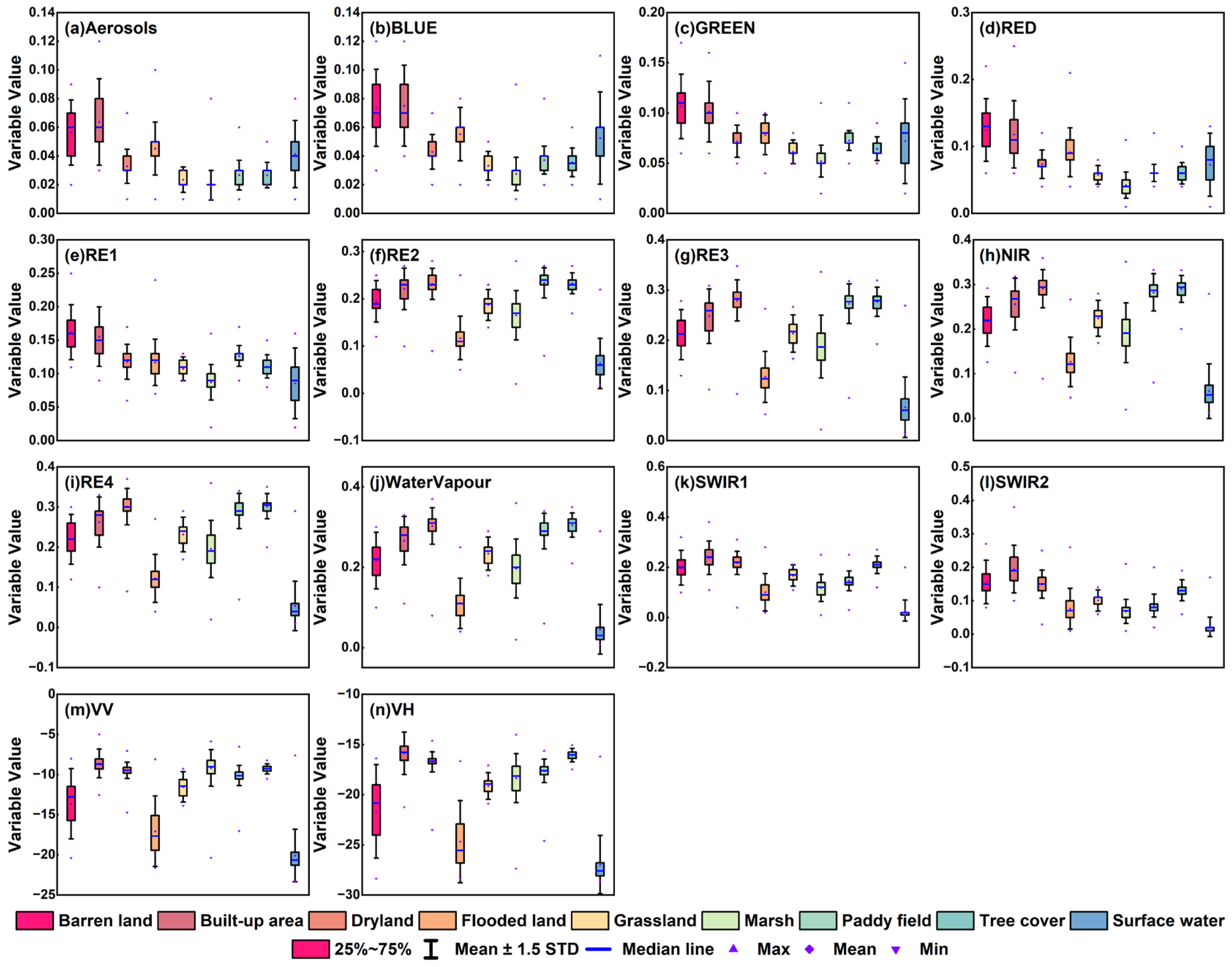
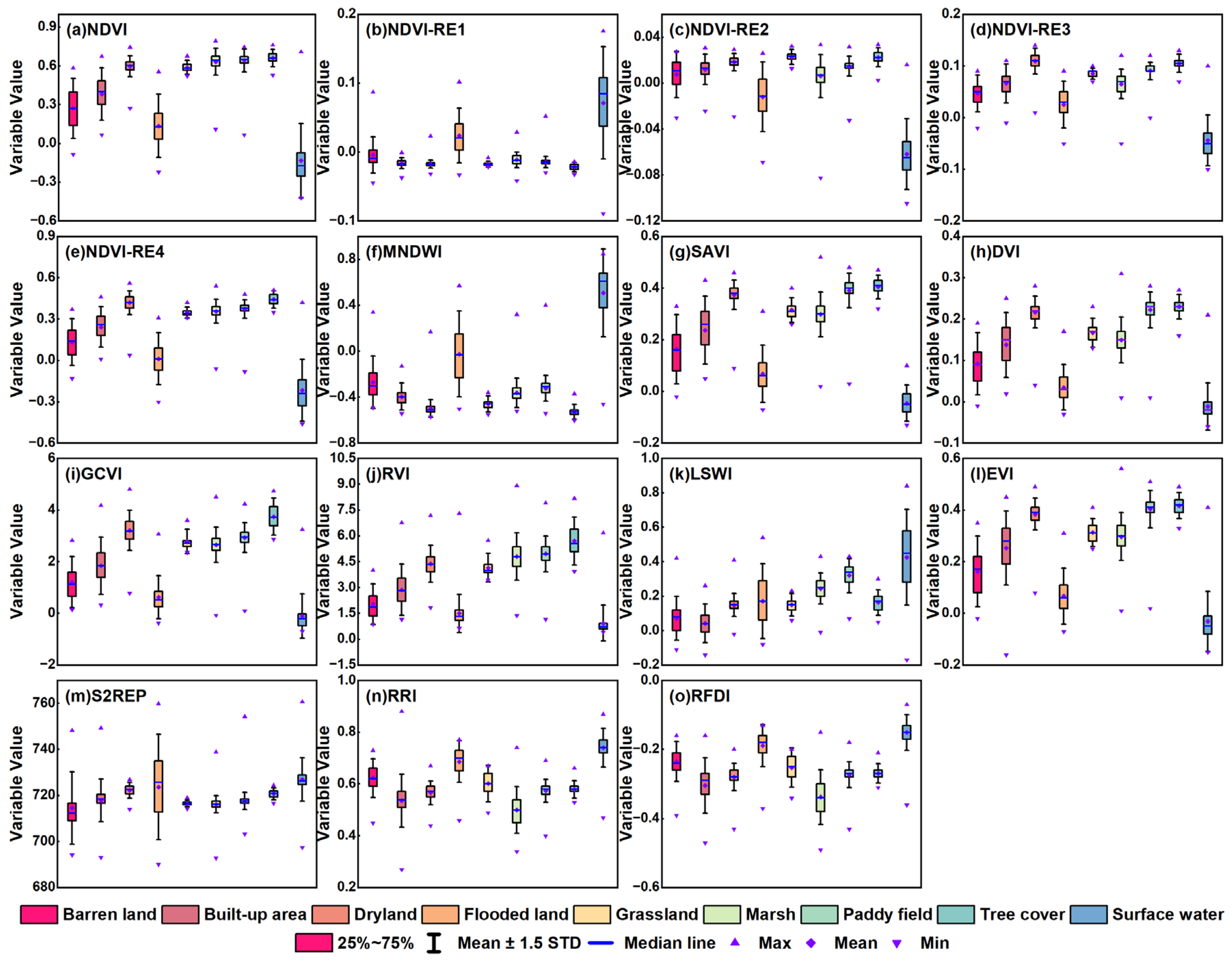
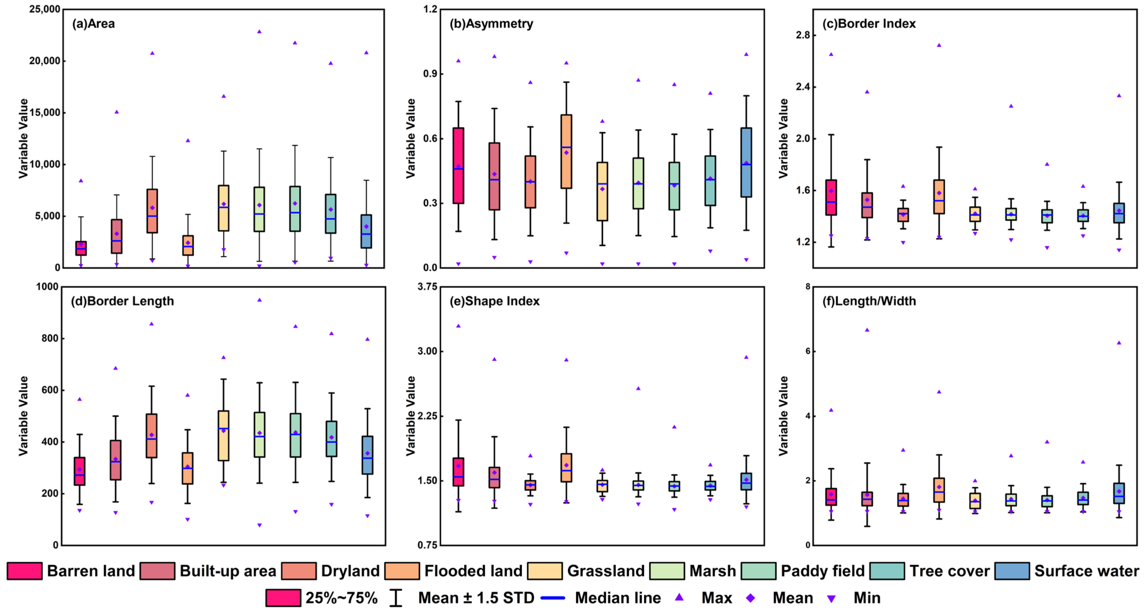
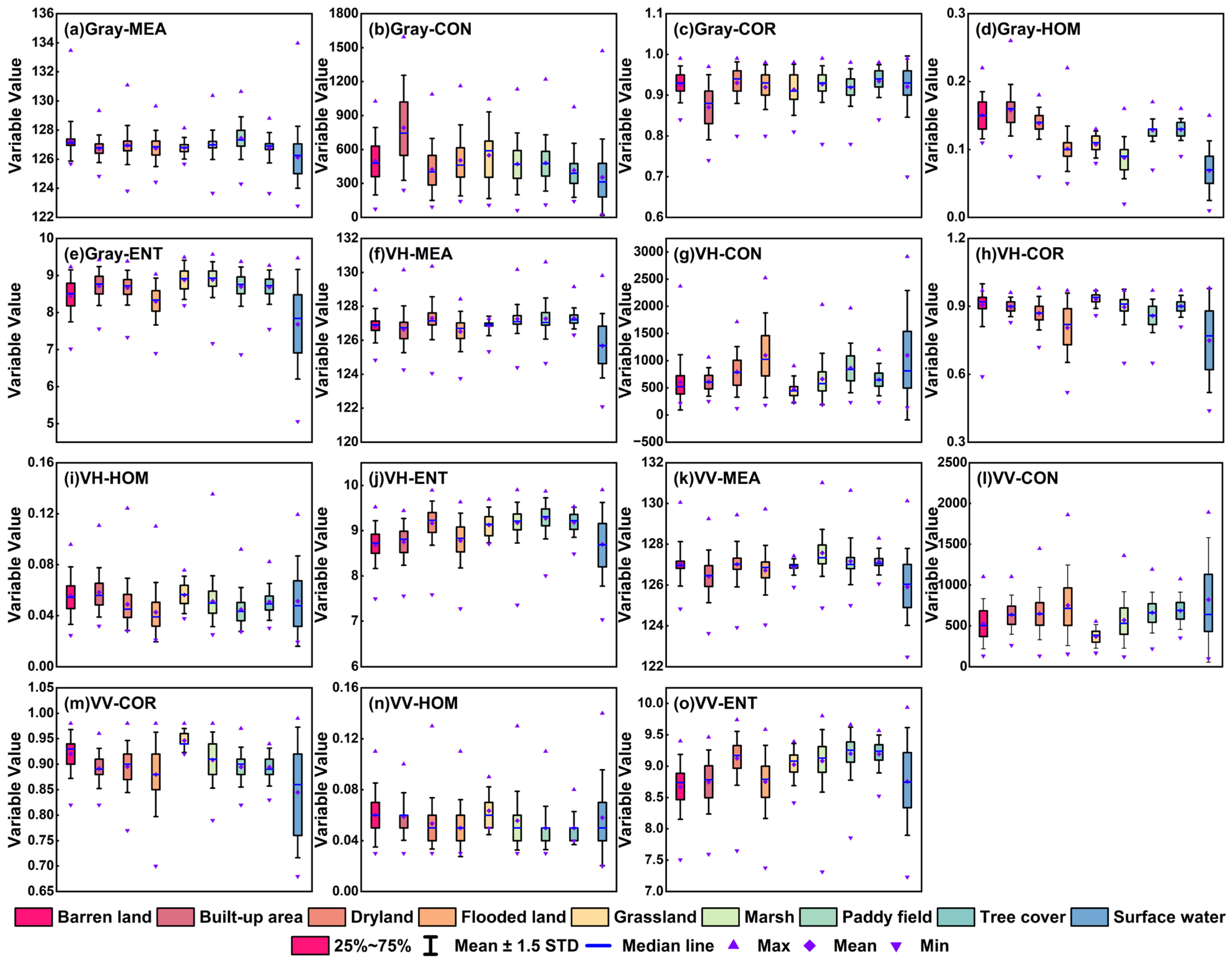
Wetland types are characterized by high soil moisture content, coverage of diverse vegetation types, and shallow water cover. Considering the wetland types in the study area, we chose abundant features to comprehensively reveal as much wetland characteristic information as possible based on previous studies [17,56,73]. Therefore, the object-based feature set includes spectral reflectance variables, microwave backscatter intensity variables, index variables, geometry variables, and texture variables. Specifically, spectral reflectance variables are extracted from Sentinel-2 images, covering a wavelength range from 443 nm to 2190 nm (i.e., Aerosols (443 nm), Blue (490 nm), Green (560 nm), Red (665 nm), RE1 (705 nm), RE2 (740 nm), RE3 (783 nm), NIR (842 nm), RE4 (865 nm), Water Vapor (940 nm), SWIR1 (1610 nm), and SWIR2 (2190 nm)). Microwave backscatter intensity variables are extracted from Sentinel-1 images (i.e., VH, VV), which were sensitive to water or soil moil moisture information [3,10,74]. Geometry variables describe the extent and shape characteristics of segmented objects, including area, asymmetry, border length, border index, shape index, and length to width ratio. Texture variables, including mean (MEA), contrast (CON), correlation (COR), homogeneity (HOM), and entropy (ENT), are generated using the Gray Level Co-occurrence Matrix (GLCM) algorithm from VV, VH and a gray band [75]. The gray band is calculated as a linear combination of the NIR, Red, and Green bands from the original Sentinel-2 images [76,77]. The calculation formulas for different indices are presented in Table 1. Moreover, the statistical plots of spectral and microwave variables, index variables, geometry variables, and texture variables are presented in Figure 2, Figure 3, Figure 4 and Figure 5, respectively. The greater the characteristic differences among ground features, the more it benefited their identification.

2.7. Dynamic Hybrid Method for Wetland Mapping

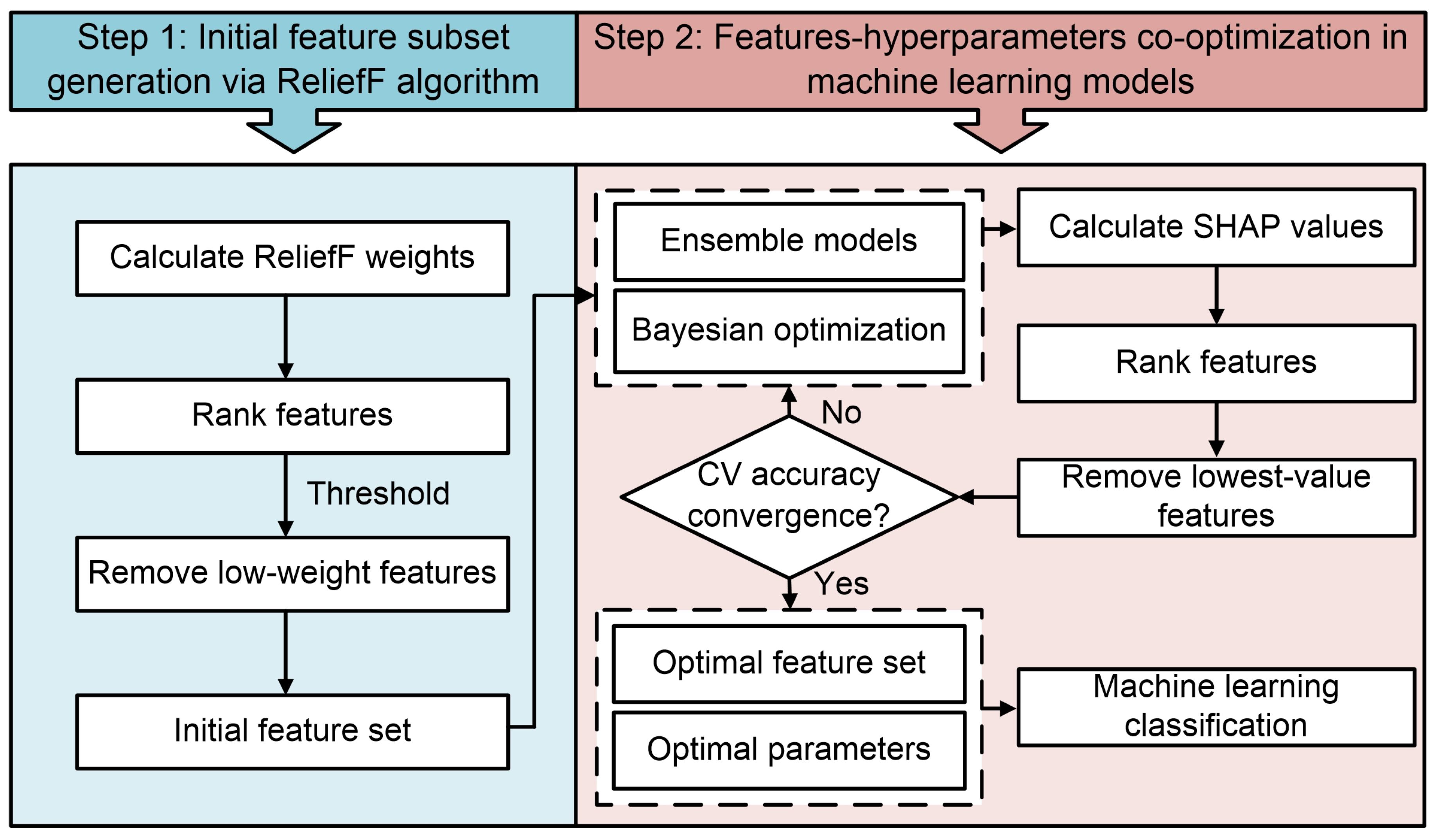
The proposed dynamic hybrid method integrating feature selection and model construction is applied to wetland mapping based on the fused Sentinel-1 and Sentinel-2 data. The process consists of two key steps: initial feature selection using the ReliefF algorithm and wetland mapping ensemble model construction based on optimized features and hyperparameters (Figure 6). In the first step, the ReliefF algorithm evaluates the entire feature set based on the calculated feature weights and removes features with weights below a predefined threshold. In the second stage, a tree-based ensemble model (i.e., RF, XGBoost, and LightGBM) is constructed using the original hyperparameters and the feature set refined by the ReliefF algorithm. Concurrently, the SHAP value for each feature is calculated during the tree-based ensemble model construction to assess feature importance. The RFE method iteratively removes the least important feature (the one with the lowest SHAP value). The ensemble model is subsequently rebuilt with the updated feature set, after which the hyperparameters are simultaneously subjected to Bayesian optimization. Cross-validation accuracy is employed to evaluate model performance at each iteration. This process is recursively repeated until either the cross-validation accuracy converges or a predefined stopping criterion (e.g., minimum number of features) is reached. The final output is an optimal feature set and the corresponding model configuration that maximizes classification performance for wetland mapping.
In this study, for the Bayesian optimization method, we used the TPE (Tree-structured Parzen Estimator) optimizer to minimize the loss of the object function. Considering the computational efficiency and model predictive performance, the maximum number of evaluations per iteration was set to 100, with iterations being terminated early if the loss value failed to decrease over 30 consecutive iterations. The hyperparameter spaces for RF, XGBoost, and LightGBM are listed in Table 2. The vital hyperparameters include the number of individual CARTs (n_estimators), learning rate of the boosting ensemble methods (learning_rate), the maximum depth of the trees (max_depth), the minimum number of samples at a leaf node (min_data_in_leaf), and the minimum sum of weights in a child (min_child_weight).

2.8. Accuracy Assessment

As confusion matrix-derived metrics, overall accuracy (OA), kappa coefficient, user’s accuracy (UA), and producer’s accuracy (PA) allow comprehensive assessments of the classification results. The overall accuracy represents the total percentage of correctly classified instances. The kappa coefficient measures the agreement between classification results and actual reference data. UA reflects the percentage of correctly classified instances within each class in the classification result, while PA denotes the percentage of correctly classified instances based on the actual reference sites for each class. These indicators can be calculated as follows:
OA = i = 1 n m i i / N
UA = m i i / m i +
PA = m i i / m + i
Kappa = N i = 1 n m i j i = 1 n m i + m + i / N 2 i = 1 n m i + m + i
where N is the total number of testing samples, mii is the number of correctly classified pixels for class i, mi+ is the total number of class i pixels in the data to be verified, m+i is the total number of type i pixels in the reference data, and n is the number of classes.

3. Results and Discussion

3.1. Feature Ranking and Accuracy Assessment Based on the ReliefF Algorithm

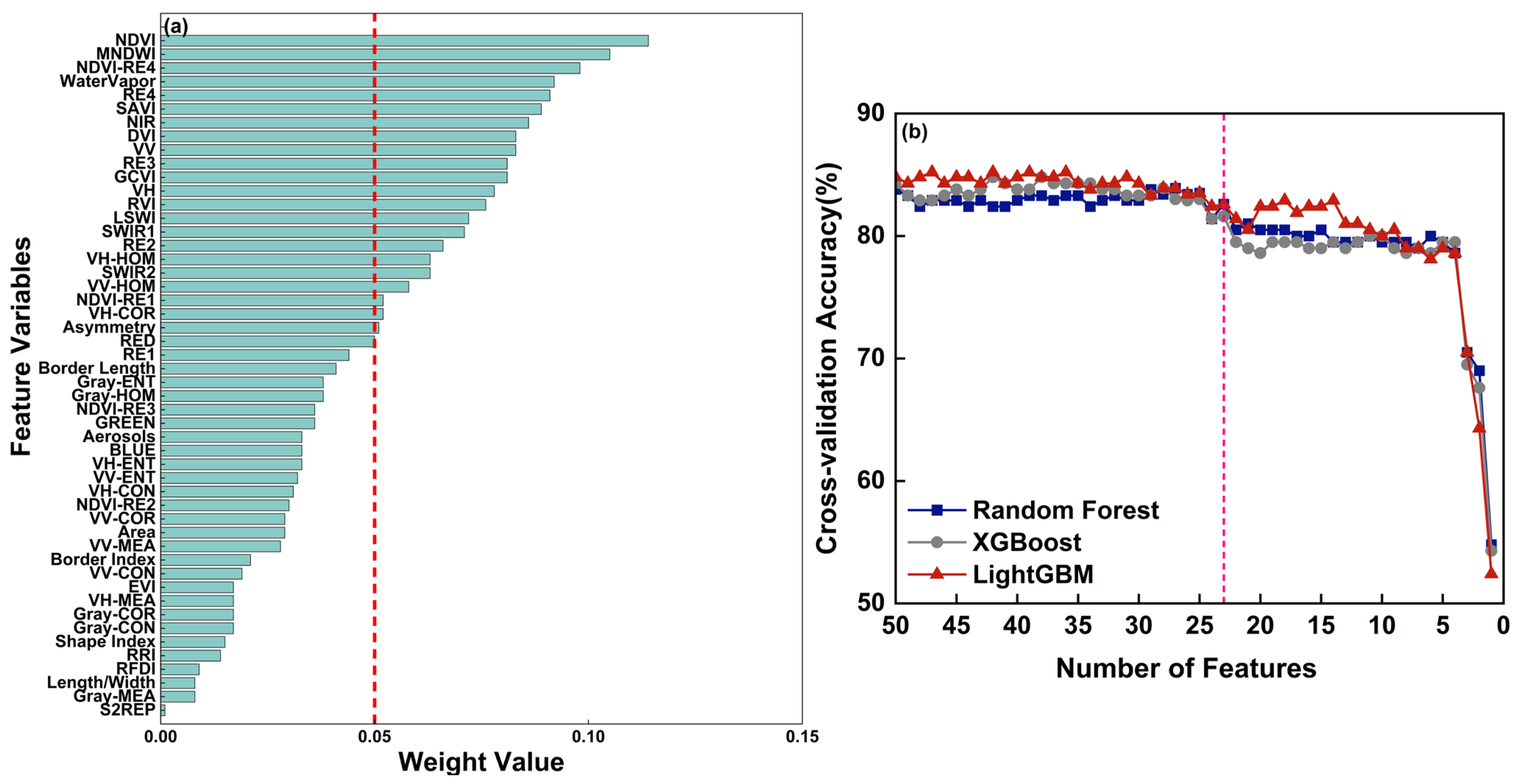
The 50 multisource features were ranked according to their ReliefF-derived weights, with a higher weight indicating greater feature importance. Features with weights below a filtering threshold of 0.05 were regarded as having a limited contribution to distinguishing various land cover types and were excluded from the original feature set.
As shown in Figure 7a, the top five most important features rank as NDVI (0.114) > MNDWI > NDVI-RE4 > B9 > B8A. Based on the 0.05 threshold, 23 features were selected. These features consisted of 10 spectral features, 3 GLCM-derived texture features, 1 object-based shape feature, and 9 spectral index features. Among the spectral features, the selected bands ranged from 644 to 1613 nm in red and infrared regions, as well as VV and VH polarized bands. Several vegetation indices, particularly various NDVIs calculated based on the red and red edge bands, were also selected. The number of shape and texture features was relatively low. Other features, including shape asymmetry, textural homogeneity and correlation of VH and VV bands, were also selected. Overall, half of the original features were eliminated using the ReliefF method.
To evaluate the predictive performance of machine learning models (i.e., RF, XGBoost, and LightGBM) using ReliefF as the sole feature selection method, one low-weight variable was sequentially removed from the feature set based on ReliefF-derived importance in descending order during each training iteration. The remaining variables were then fed into the models for training until all variables were filtered out. During the training process, hyperparameter tuning was performed using the widely applied grid search method. Figure 7b shows the cross-validation accuracy of RF, XGBoost, and LightGBM models with ReliefF-based variables and optimal hyperparameters. The RF, XGBoost, and LightGBM achieved the highest predictive accuracy when using 50, 42, and 42 features, with the cross-validation accuracy being 83.8%, 84.8%, and 85.2%. As the number of remaining features was filtered down to 23, cross-validation accuracy decreased slightly with fluctuations, while the feature dimensionality was significantly reduced. Once the number of features dropped below 23, further reductions in features led to significant fluctuations in accuracy.
The result illustrates that the filter-based selection of ReliefF, effectively reduces the dimensionality of the feature space by feature evaluation according to the inherent statistical properties of the data. The selected features maintain data diversity and information richness. Moreover, the extensive feature removal indicates relatively high data redundancy among the features, possibly resulting from extracting features from the same satellite images. Therefore, feature selection is imperative to enhance data effectiveness and improve the performance of classification models.

3.2. Evaluation of Hyperparameter Tuning Methods

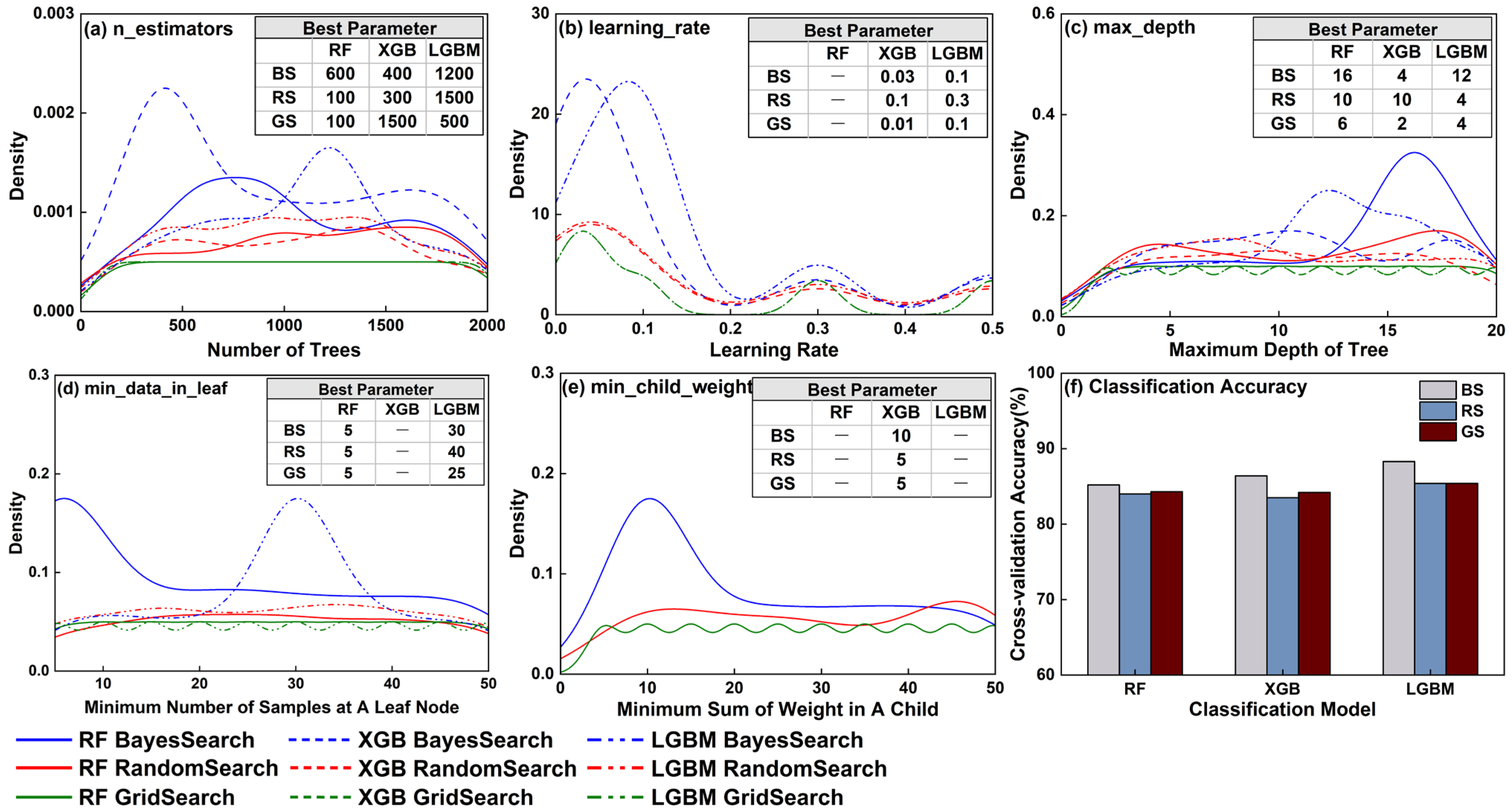
The effectiveness of three hyperparameter tuning methods, i.e., grid search (GS), random search (RS), and Bayesian optimization (BS), in optimizing RF, XGBoost, and LightGBM models was evaluated through a comparative analysis using features filtered by ReliefF. The vital parameters were selected, for fine-tuning to improve model performance. The ‘n_estimators’ parameter controls the number of individual CARTs that contribute to the final prediction and influence the model’s efficiency. The ‘learning_rate’ parameter of the boosting ensemble methods, i.e., XGBoost and LightGBM, controls the model update step size at each iteration, based on the errors produced by previous predictions. The ‘max_depth’, ‘min_data_in_leaf’, and ‘min_child_weight’ parameters control the maximum depth of the trees, the minimum number of samples at a leaf node, and the minimum sum of weights in a child, respectively. These parameters determine the structure of individual trees and directly influence the generalization ability and robustness of the model. A unified domain space was defined to represent the range of the parameters.
Figure 8a–e show kernel density estimate curves for various hyperparameters. The best parameters for the various machine learning algorithms differed significantly depending on the tuning method. Bayesian optimization identified the best parameters from the frequently occurring hyperparameter values within the domain space. Although random search found some frequently occurring hyperparameter values, it determined the best parameters randomly, which might fall outside of the high-probability range. With grid search, the probability of the occurring parameter values was uniformly distributed. As illustrated in Figure 8f, the RF, XGBoost, and LightGBM models, with hyperparameter tuning via Bayesian optimization, achieved the highest cross-validation accuracy (85.2–88.3%). The accuracy of models optimized through grid search method was slightly higher than that of models optimized using random search.
The cross-validation accuracy demonstrates the greater efficiency of Bayesian optimization in finding the global optimum within the hyperparameter space, thereby enhancing model performance. By focusing more on promising hyperparameters, Bayesian optimization allows for a more targeted and efficient search. Compared to grid search and random search with greater spatial and temporal computational complexities, Bayesian optimization demonstrates significantly reduced search time and advantages for high-dimensionality hyperparameter spaces. Therefore, Bayesian optimization is a powerful tool for tuning machine learning models.

3.3. Evaluation of Dynamic Hybrid Methods

Figure 9 presents the cross-validation accuracy of the proposed dynamic hybrid methods using RF, XGBoost, and LightGBM models with varying numbers of features optimized by the RFE method for each iteration. Initially, 23 features selected by the ReliefF method were input into the models, and the hyperparameters of different models were optimized through Bayesian optimization method in each iteration. In addition, the SHAP method was evaluated against ReliefF-based, tree-based and permutation-based feature importance analysis methods to demonstrate its effectiveness. Tree-based models derive feature importance based on the mean decrease in impurity. In contrast, permutation-based models assess feature importance by measuring the changes in model performance under randomly shuffled feature values.
According to Figure 9, the accuracy of the three models shows a similar trend with fluctuations. Compared to the accuracy of models with the original feature set, although approximately half of the original features were filtered out using ReliefF method, the accuracy remains relatively stable or improves slightly as the number of features decreases. This indicated that the original feature set contained numerous redundant features, which exerted a negative impact on the model’s predictive accuracy and operational efficiency. The accuracy dramatically declined when the number of features fell below 8. All three models achieved the highest accuracy (84.8–88.2%) by using 8 to 23 features based on SHAP importance, followed by those using features selected according to tree-based importance (83.2–87.2%) and permutation-based importance (79.0–85.2%), and ReliefF-based importance (79.7–85.0%).
According to the illustrated results, the features identified initially filtered by the ReliefF algorithm still require further optimization to improve model performance, whereas features selected based on SHAP importance achieve superior model performance. Furthermore, Figure 9 showed that the models with ReliefF-selected features achieved the lowest accuracy. This result indicated that models using features filtered exclusively based on inherent data properties underperformed compared to those relying on algorithm-specific feature sets. The RFE algorithm is a wrapper-based feature selection method that relies on a specific classifier. In the proposed method, the RFE method was employed to automatically select the appropriate features based on classification accuracy, thereby avoiding biases resulting from the manual selection of top-ranked features based on their importance. SHAP values provide local explanations for tree-based models, resulting in a more accurate understanding of the model’s behavior [61]. SHAP values offer advantages in evaluating feature contributions to the models, serving as an effective tool for feature selection.
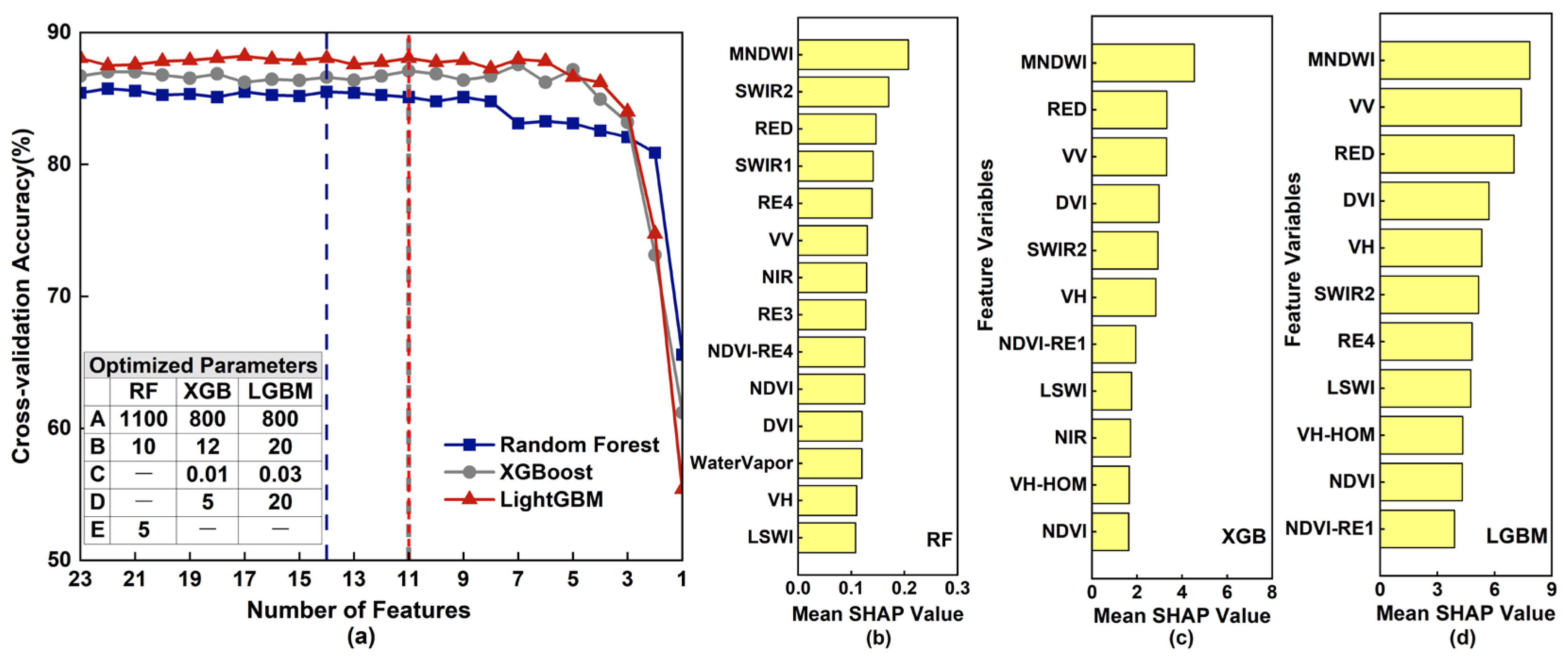
Figure 10a shows the cross-validation accuracy of RF, XGBoost, and LightGBM models with varying numbers of features selected based on SHAP importance. The final optimized features were selected as the cross-validation accuracy stabilized without significant increases. As a result, 14 features were selected for the RF model, achieving an accuracy of 85.5%. In contrast, 11 features were selected for both the XGBoost and LightGBM models, which achieved accuracies of 87.1% and 88.0%, respectively. The feature selection method combining ReliefF and RFE algorithms with SHAP values as a feature evaluation criterion (ReliefF-RFE-SHAP) ultimately yields an optimal feature set, consisting of approximately 20–30% of the original features. Integrating filter and wrapper selection methods effectively removes redundant features, decreases data dimensionality, and enhances model performance.
Regarding the hyperparameter optimization results for models with optimal features, the RF method used the highest number of CARTs, with the ‘n_estimators’ parameter set to 1100. In contrast, both XGBoost and LightGBM employed 800 individual CARTs. The LightGBM model configured individual CARTs with a maximum depth of 20, while RF and XGBoost used depths of 10 and 12, respectively. Both XGBoost and LightGBM were boosting ensemble algorithms. However, LightGBM employed a higher learning rate of 0.03, which allowed for faster convergence. Due to the dynamic hybrid method adopted, the hyperparameters with Bayesian optimization vary for models with different features at each iteration. This dynamic optimization approach facilitated better adaptation of model hyperparameters to varying feature data, which ensured the model was optimal under the current feature and parameter conditions and resulted in an effective improvement in model performance. The cross-validation accuracy demonstrates that the Bayesian-optimized LightGBM model (BO-LightGBM) using features selected by ReliefF-RFE-SHAP can efficiently produce superior results with fewer features than the RF and XGBoost models.
As shown in Figure 10b–d, the optimized features and their importance scores (represented by mean SHAP values) differ among the various models. This demonstrated the importance of selecting features based on the specified algorithms. Several variables with high importance scores were frequently selected from the 23 initial features across all three models, including MNDWI, RED, VV, SWIR2, DVI, VH, LSWI, and NDVI. Furthermore, other features (RE4, NIR, NDVI-RE1, and VH-HOM) also demonstrated high importance in two of the models.

3.4. Assessment of Computational Efficiency

Table 3 shows the computation time of different methods based on non-feature selection and feature selection. The results showed that models without feature selection and with hyperparameter optimization via grid search consumed excessive time, which was 2 to 4 times longer than that of models with feature selection and hyperparameter optimization using via Bayesian search. BO-LightGBM model with ReliefF-RFE-SHAP-selected features exhibited significant efficiency, with a computation time of 0.904 h, which was slightly higher than that of the LightGBM model with tree-selected features. This analysis was conducted on a computer with the following configuration: CPU, Intel(R) Core(TM) i5-8265U; Installed RAM, 16.0 GB.

3.5. Classification Results

Figure 11 shows the confusion matrix of the dynamic hybrid methods using RF, XGBoost, and LightGBM models, which are applied to classify land cover types, including barren land, built-up area, dryland, flooded land, grassland, marsh, paddy field, tree cover, and surface water within the study area. The results showed that object-based methods outperformed pixel-based methods. The overall accuracies of RF, XGBoost, and LightGBM were below 85%. The object-based LightGBM method yielded the highest overall accuracy and kappa coefficient (OA = 89.4%, kappa = 0.875), followed by XGBoost (OA = 87.8%, kappa = 0.856) and RF (OA = 85.1%, kappa = 0.823).
For object-based methods, in terms of wetland types, the accuracies for marsh, paddy field, and surface water types were high across all three machine learning models, reaching as high as 86% or even higher. In contrast, the classification accuracy for the flooded land type was relatively lower in the RF model (below 80%). Notably, LightGBM achieved the highest producer’s and user’s accuracies among all models (PA = 93.8%, UA = 87.9% for marsh; PA = 91.3%, UA = 94.8% for paddy field; PA = 92.7%, UA = 93.9% for surface water; PA = 86.5%, UA = 80.0% for flooded land). In terms of non-wetland types, the classification accuracy for grassland was the lowest (PA < 65%). The results also showed that object-based methods produced higher PA and UA for most classes than pixel-based methods.
Comparative analysis revealed the superior classification performance of LightGBM, which accurately distinguished wetland and non-wetland types with high accuracy. Nevertheless, LightGBM demonstrated notable misclassification, i.e., the confusion between paddy field and dryland, as well as between dryland field and tree cover. Additionally, the flooded land was predominantly misclassified as barren land and surface water. Significant confusions were observed with marsh being misclassified as grassland and paddy field.
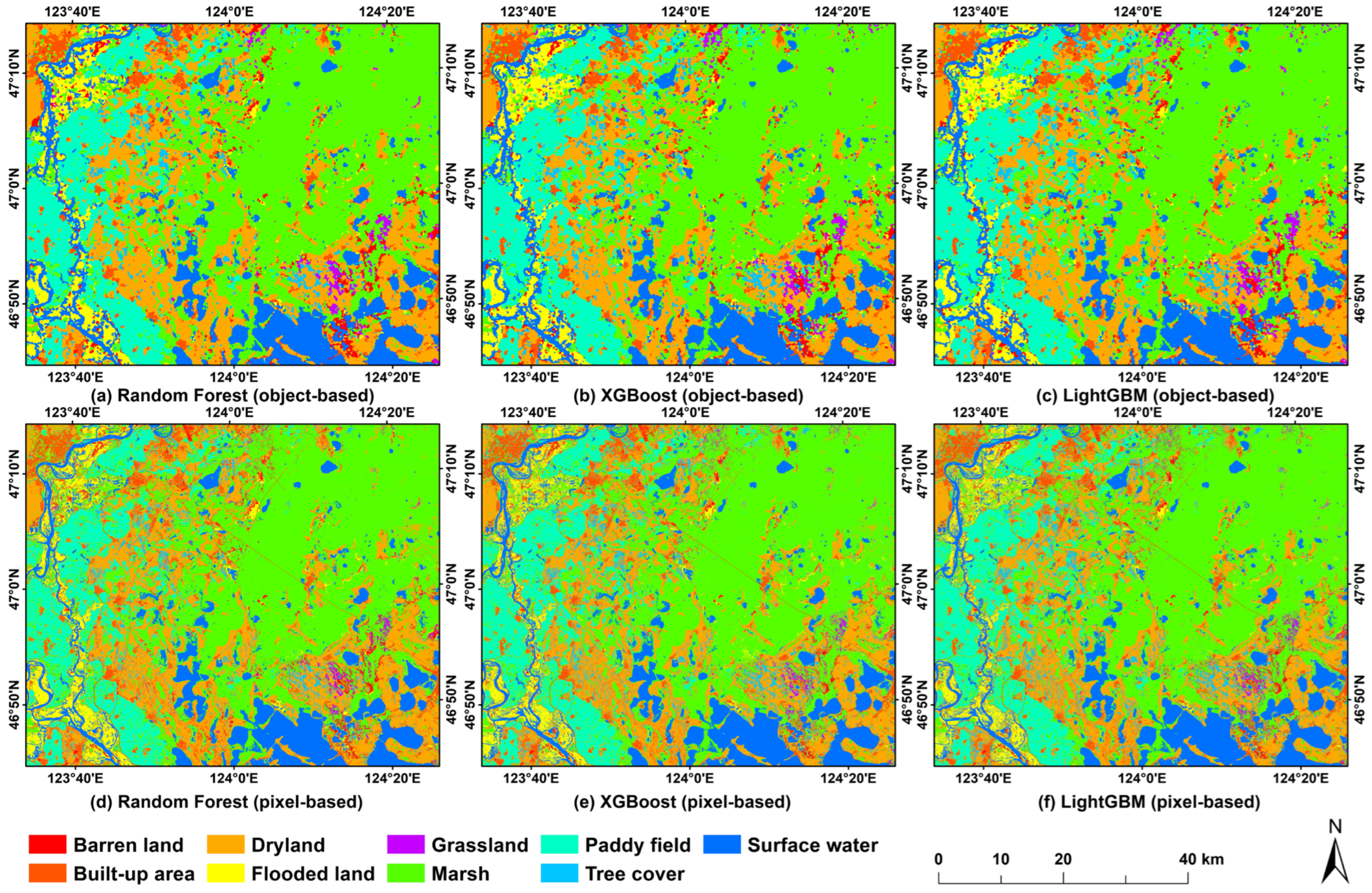
As illustrated in Figure 12, the object-based classification maps generated by the RF, XGBoost, and LightGBM models can correctly reveal the spatial distribution patterns of different land covers. Compared to pixel-based methods, these maps effectively mitigated the impact of isolated pixels, which disrupted the spatial continuity of ground objects and also reduced the classification accuracy. Finer segmentation scales facilitate the capture of more detailed land cover characteristics, but excessively fragmented objects can increase misclassification risks and compromise computational efficiency. Research proved that the object-based segmentation scale directly affects the model performance and computational efficiency. Fragmented land covers, such as cultivated fields scattered across vast marshlands, flooded areas along rivers, and dispersed tree and grasslands, were prone to misclassification, particularly in the results of the RF model. The boosting ensemble methods demonstrated superior performance, particularly LightGBM, which reduced the probability of misclassification.
To sum up, the object-based BO-LightGBM model with ReliefF-RFE-SHAP-selected features achieved better prediction accuracy and generated a more reliable classification map. However, the classification results exhibited certain limitations. Specifically, owing to the land cover types in the study area, the proposed method clearly demonstrated better performance in classifying herbaceous marsh wetlands, floodplain wetlands, surface water, and constructed wetlands. Although the classification effectiveness for other wetland types could not be verified, the proposed method exhibited strong universality, which enabled it to be applied to solve similar problems. Moreover, Some wetland types and non-wetland types were misclassified, such as grasslands and marsh wetlands, as well as scattered non-wetland types (e.g., grassland, trees, and barren lands) and their adjacent wetland types. In this study area, marsh wetlands were the dominant land cover type, with wetland vegetation dominated by herbs. Some grasslands were distributed adjacent to wetlands, which resulted in blurred boundaries between these two types. During the multi-scale segmentation process, a single object was likely to contain pixels belonging to multiple land cover types, thus causing classification errors. Similarly, some scattered land cover types with fragmented spatial patterns might also exert a comparable influence during segmentation process. Furthermore, the insufficient samples for these land cover types with small distribution areas led to difficulty for machine learning classifiers in adequately mining data information, resulting in lower classification accuracy. Thus, more efforts would be devoted to acquiring sufficient higher-quality samples, enriching features (e.g., multi-temporal feature variables), and using higher-resolution images, which may provide advantages for enhancing model performance and improving classification accuracy.

3.6. Explanation of Variable Importance for Wetland Classification

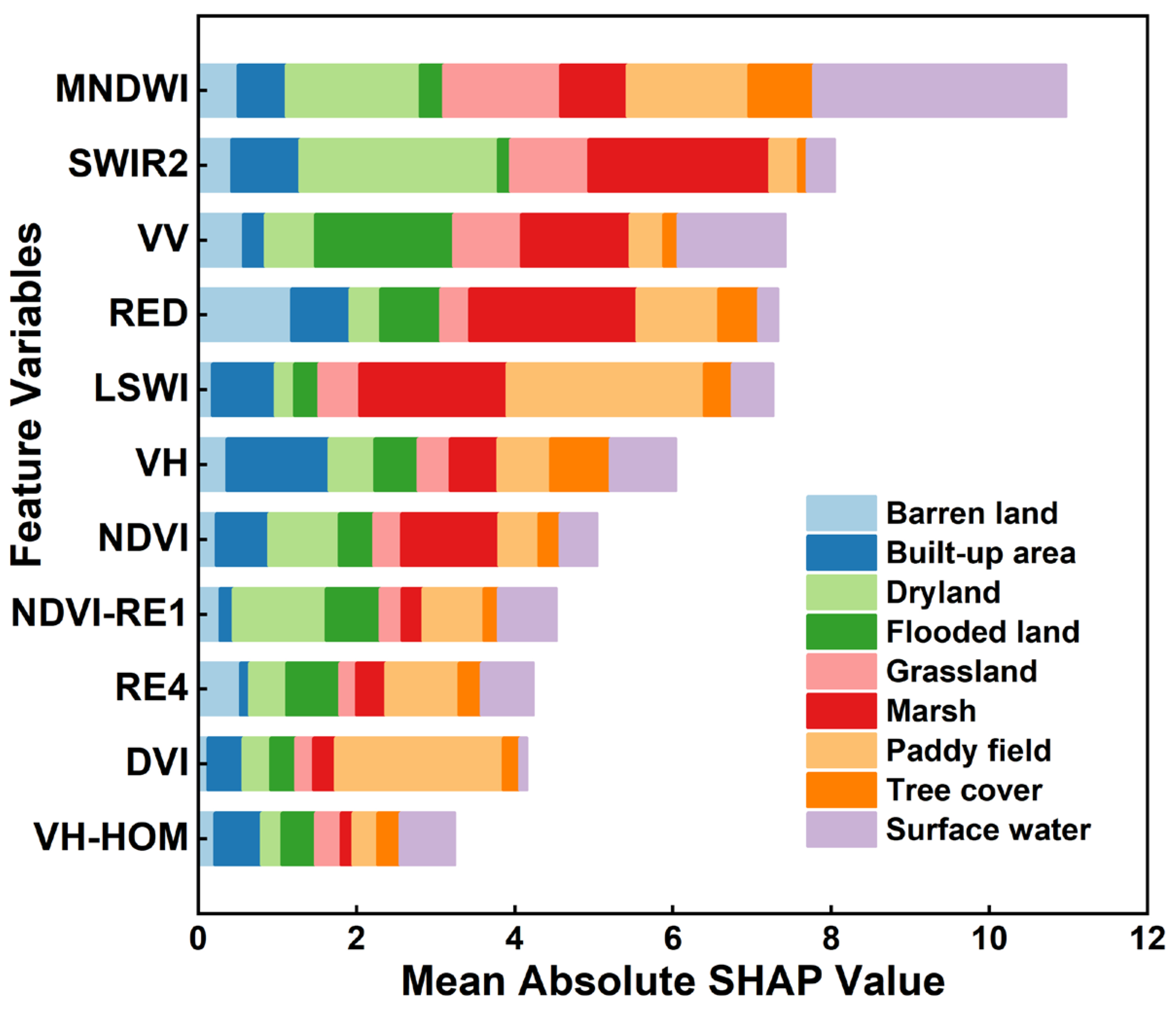
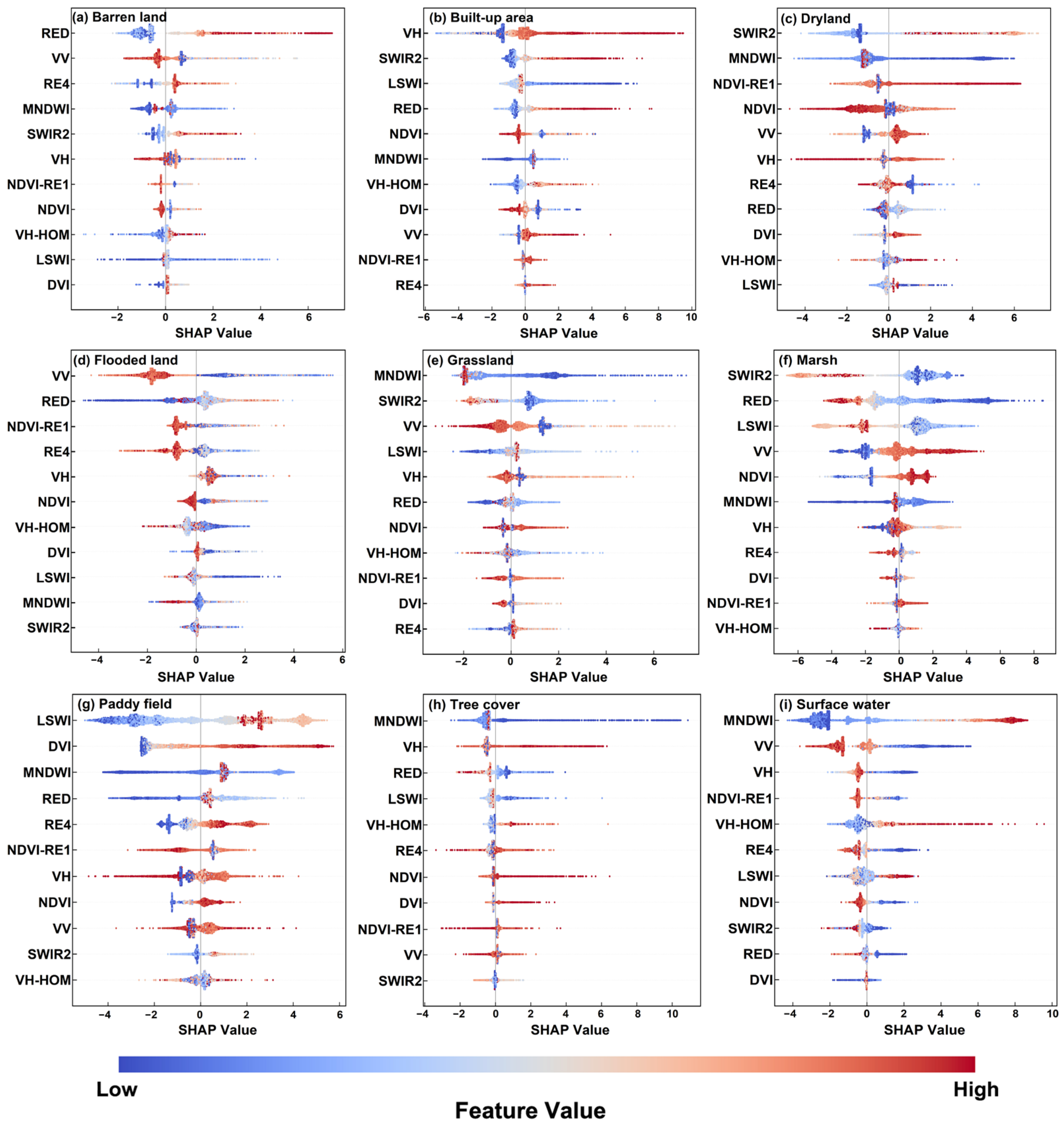
SHAP values were used to interpret the model, providing a deeper understanding of the contribution of various features to wetland classification. Figure 13 displays the mean absolute SHAP values for optimal features across different land cover types in the LightGBM model, ranked by feature contributions. Figure 14 shows the SHAP values of individual samples to reveal the feature contributions. The blue and red points represent the lower and higher feature values, respectively. The horizontal position reflects whether a feature positively or negatively influences the classification results. A wider color region indicates that the feature has a greater influence on the classification results. As shown in Figure 13 and Figure 14, the SHAP values provide global and local explanations for the model’s output. For each class, Figure 15 presented the feature pairs with the most significant interactivity. In terms of wetland types.
In general, MNDWI, SWIR2, VV, RED, LSWI, and VH contributed more to the classification results of the LightGBM model, with SHAP values exceeding 5.0. In terms of wetland types, water normalized indices (MNDWI and LSWI) with higher feature values contributed significantly to the identification of surface water and paddy field, with the mean absolute SHAP values of 3.20 and 2.50, respectively. MNDWI and NDVI-RE1 had strong interactions for water identification (Figure 15r). Higher values of MNDWI and lower values of NDVI-RE1 exerted a positive influence on the classification accuracy. MNDWI and LSWI were typical and widely used indices for water or moisture information extraction, which had been demonstrated to effectively identify water and non-water regions. As constructed wetlands, paddy fields exhibited relatively high soil moisture content, and their surrounding areas were mostly drylands and barren lands. Thus, these indices enabled the effective distinction of paddy fields and other non-wetland regions.
The VV polarization feature was more sensitive to flooded land, with the highest mean absolute SHAP value of 1.75. Lower feature values of VV resulted in better classification results for flooded land. VV and VH values exhibited relatively strong interactivity, and lower values of both were more conducive to extraction for flooded land (Figure 15h). In the floodplain, the areas were submerged under shallow water. These submerged areas exhibited weak backscattering signals, as specular reflection occurred when they interacted with microwaves. The floodplain areas appeared as dark areas, which formed a distinct contrast with the bright areas of non-floodplain regions. This contrast ultimately facilitated the identification of the flooded areas. Moreover, VV also played an important role in marsh identification, as it exhibited strong interactivity with NDVI (Figure 15I).
As a spectral feature, a lower SWIR2 value positively influenced the classification results for marsh, achieving a mean absolute SHAP value of 2.29. This could be attributed to the fact that marsh wetlands were characterized by high soil and vegetation water content, which exerted strong absorption on the SWIR2 spectrum, resulting in regions with lower reflectance values compared to non-wetland areas. Other features, like RED, NDVI, NDVI-RE1, RE4, DVI, and VH also proved crucial for recognizing wetland types, ranking among the top five based on mean absolute SHAP values. These features could provide abundant vegetation information to facilitate the distinction between wetland types and non-vegetation areas. Vegetation indices played an important role due to the strong interactivity of each other for wetland classification (Figure 15).
Although DVI had a lower mean absolute SHAP value for overall classification, it was more sensitive to paddy land due to its strong interactivity with NDVI and RE4, with a higher mean absolute SHAP value of 2.12 (Figure 15m,n). VH-HOM, as the only texture feature selected, demonstrated greater sensitivity in classifying surface water, achieving a SHAP value of 0.69. Higher VH-HOM values also exerted a considerable positive impact on the identification of surface water. For non-wetland classes, RED, VH, SWIR2, and MNDWI were more effective in identifying barren land, built-up area, dryland, and grassland, with higher mean absolute SHAP values of 1.18, 1.29, 2.51, and 1.48, respectively.
The global and local explanations based on SHAP values revealed the model’s dependence on the input features. This understanding enables developers to determine the most critical features for enhancing model performance by highlighting their specific contributions. Features extracted from Sentinel-2 images, such as spectral reflectance features and normalized indices, provide valuable information about the vegetation characteristics of wetland types, particularly in the red and infrared bands. Moreover, features extracted from Sentinel-1 images are particularly effective in distinguishing wetland types characterized by pronounced hydrological properties. Combining Sentinel-1 and Sentinel-2 data demonstrates significant advantages in wetland mapping.

4. Conclusions

This study proposed a dynamic hybrid method combining feature selection and ensemble model construction to enhance wetland mapping based on Sentinel-1 and Sentinel-2 data fusion. The selection method integrated ReliefF and RFE algorithms with a SHAP-based feature evaluation criterion to effectively reduce the complexity of high-dimensional feature spaces. The selected optimal features contributed significantly to model performance. The Bayesian-optimized LightGBM model with fewer features achieved superior wetland classification performance to the RF and XGBoost models, yielding the highest overall accuracy of 89.4% and a kappa coefficient of 0.875.
SHAP values offered global and local interpretations of the model to better understand the contribution of various features to wetland classification. SHAP value analysis demonstrated the complementary advantages of integrating Sentinel-1 and Sentinel-2 data for wetland classification. Spectral features derived from the red and infrared bands of Sentinel-2 images were particularly effective in characterizing vegetation characteristics of various wetland types, while features derived from Sentinel-1 images demonstrated greater utility for capturing hydrological characteristics.
The object-oriented classification maps generated by the BO-LightGBM model with ReliefF-RFE-SHAP-selected features correctly revealed the spatial distribution patterns of different land covers. The proposed dynamic hybrid method offered an effective tool for wetland mapping and contributed to wetland environmental monitoring and management.
Future efforts will focus on the scalability of the proposed approach in larger geographic ranges and assess its applicability for refined wetland mapping globally. Additionally, attempts will be made to implement the entire hybrid algorithmic workflow on cloud platforms to improve large-scale wetland mapping, which may contribute significantly to the research on global wetland ecosystems.

Author Contributions

Conceptualization, Y.M. (Yue Ma); methodology, Y.M. (Yue Ma) and Y.M. (Yongchao Ma); software, Q.Z. and Q.C.; validation, Q.Z. and Q.C.; formal analysis, Y.M. (Yue Ma); investigation, Y.M. (Yongchao Ma), Q.Z. and Q.C.; resources, Y.M. (Yue Ma); writing—original draft preparation, Y.M. (Yue Ma); writing—review and editing, Y.M. (Yue Ma) and Y.M. (Yongchao Ma); visualization, Q.Z. and Q.C.; and supervision, Y.M. (Yue Ma). All authors have read and agreed to the published version of the manuscript.

Funding

This research was funded by the National Natural Science Foundation of China, grant number 42201433.

Data Availability Statement

The Sentinel-2 dataset is available through the Google Earth Engine platform (https://developers.google.com/earth-engine/datasets (accessed on 2 May 2024)).

Conflicts of Interest

The authors declare no conflicts of interest.

References

  1. Bridgewater, P.; Kim, R.E. The Ramsar convention on wetlands at 50. Nat. Ecol. Evol. 2021, 5, 268–270. [Google Scholar] [CrossRef]
  2. Ramsar, C.S. The Ramsar Convention Manual: A Guide to the Convention on Wetlands (Ramsar, Iran, 1971), 6th ed.; Ramsar Convention Secretariat: Gland, Switzerland, 2013. [Google Scholar]
  3. Liu, H.; Jiang, Q.; Ma, Y.; Yang, Q.; Shi, P.; Zhang, S.; Tan, Y.; Xi, J.; Zhang, Y.; Liu, B.; et al. Object-Based Multigrained Cascade Forest Method for Wetland Classification Using Sentinel-2 and Radarsat-2 Imagery. Water 2022, 14, 82. [Google Scholar] [CrossRef]
  4. Xu, T.; Weng, B.; Yan, D.; Wang, K.; Li, X.; Bi, W.; Li, M.; Cheng, X.; Liu, Y. Wetlands of International Importance: Status, Threats, and Future Protection. Int. J. Environ. Res. Public Health 2019, 16, 1818. [Google Scholar] [CrossRef] [PubMed]
  5. Mahdavi, S.; Salehi, B.; Granger, J.; Amani, M.; Brisco, B.; Huang, W. Remote sensing for wetland classification: A comprehensive review. Gisci. Remote Sens. 2017, 55, 623–658. [Google Scholar] [CrossRef]
  6. Eppink, F.V.; van den Bergh, J.C.; Rietveld, P. Modelling biodiversity and land use: Urban growth, agriculture and nature in a wetland area. Ecol. Econ. 2004, 51, 201–216. [Google Scholar] [CrossRef]
  7. Mondal, B.; Dolui, G.; Pramanik, M.; Maity, S.; Biswas, S.S.; Pal, R. Urban expansion and wetland shrinkage estimation using a GIS-based model in the East Kolkata Wetland, India. Ecol. Indic. 2017, 83, 62–73. [Google Scholar] [CrossRef]
  8. Guo, M.; Li, J.; Sheng, C.; Xu, J.; Wu, L. A review of wetland remote sensing. Sensors 2017, 17, 777. [Google Scholar] [CrossRef]
  9. Chaudhary, R.K.; Puri, L.; Acharya, A.K.; Aryal, R. Wetland mapping and monitoring with Sentinel-1 and Sentinel-2 data on the Google Earth Engine. J. For. Nat. Resour. Manag. 2023, 3, 1–21. [Google Scholar] [CrossRef]
  10. Peng, K.; Jiang, W.; Hou, P.; Wu, Z.; Ling, Z.; Wang, X.; Niu, Z.; Mao, D. Continental-scale wetland mapping: A novel algorithm for detailed wetland types classification based on time series Sentinel-1/2 images. Ecol. Indic. 2023, 148, 110113. [Google Scholar] [CrossRef]
  11. Kaplan, G.; Avdan, Z.Y.; Avdan, U. Mapping and monitoring wetland dynamics using thermal, optical, and SAR remote sensing data. Wetl. Manag. Assess. Risk Sustain. Solut. 2019, 87, 86–107. [Google Scholar] [CrossRef]
  12. Liang, Y.; Zhang, L.; Xiong, S.; You, L.; He, Z.; Huang, Y.; Lu, J. C-band synthetic aperture radar time-series for mapping of wetland plant communities in China’s largest freshwater lake. J. Appl. Remote Sens. 2025, 19, 021006. [Google Scholar] [CrossRef]
  13. Grings, F.; Ferrazzoli, P.; Karszenbaum, H.; Salvia, M.; Kandus, P.; Jacobo-Berlles, J.; Perna, P. Model investigation about the potential of C band SAR in herbaceous wetlands flood monitoring. Int. J. Remote Sens. 2008, 29, 5361–5372. [Google Scholar] [CrossRef]
  14. Prasad, P.; Loveson, V.J.; Kotha, M. Probabilistic coastal wetland mapping with integration of optical, SAR and hydro-geomorphic data through stacking ensemble machine learning model. Ecol. Inform. 2023, 77, 102273. [Google Scholar] [CrossRef]
  15. Landuyt, L.; Verhoest, N.E.; Van Coillie, F.M. Flood mapping in vegetated areas using an unsupervised clustering approach on sentinel-1 and-2 imagery. Remote Sens. 2020, 12, 3611. [Google Scholar] [CrossRef]
  16. Konapala, G.; Kumar, S.V.; Ahmad, S.K. Exploring Sentinel-1 and Sentinel-2 diversity for flood inundation mapping using deep learning. ISPRS J. Photogramm. 2021, 180, 163–173. [Google Scholar] [CrossRef]
  17. Slagter, B.; Tsendbazar, N.-E.; Vollrath, A.; Reiche, J. Mapping wetland characteristics using temporally dense Sentinel-1 and Sentinel-2 data: A case study in the St. Lucia wetlands, South Africa. Int. J. Appl. Earth Obs. 2020, 86, 102009. [Google Scholar] [CrossRef]
  18. Mohseni, F.; Amani, M.; Mohammadpour, P.; Kakooei, M.; Jin, S.; Moghimi, A. Wetland mapping in great lakes using Sentinel-1/2 time-series imagery and DEM data in Google Earth Engine. Remote Sens. 2023, 15, 3495. [Google Scholar] [CrossRef]
  19. Gallant, A.L. The challenges of remote monitoring of wetlands. Remote Sens. 2015, 7, 10938–10950. [Google Scholar] [CrossRef]
  20. Wen, L.; Hughes, M. Coastal wetland mapping using ensemble learning algorithms: A comparative study of bagging, boosting and stacking techniques. Remote Sens. 2020, 12, 1683. [Google Scholar] [CrossRef]
  21. Ferreira, C.S.; Kašanin-Grubin, M.; Solomun, M.K.; Sushkova, S.; Minkina, T.; Zhao, W.; Kalantari, Z. Wetlands as nature-based solutions for water management in different environments. Curr. Opin. Environ. Sci. Health 2023, 33, 100476. [Google Scholar] [CrossRef]
  22. Carlson, K.; Buttenfield, B.P.; Qiang, Y. Wetland Classification, Attribute Accuracy, and Scale. ISPRS Int. J. Geo-Inf. 2024, 13, 103. [Google Scholar] [CrossRef]
  23. Adam, E.; Mutanga, O.; Rugege, D. Multispectral and hyperspectral remote sensing for identification and mapping of wetland vegetation: A review. Wetl. Ecol. Manag. 2010, 18, 281–296. [Google Scholar] [CrossRef]
  24. Yuling, H.; Gang, Y.; Weiwei, S.; Lin, Z.; Ke, H.; Xiangchao, M. Wetlands mapping in typical regions of South America with multi-source and multi-feature integration. J. Remote Sens. 2023, 27, 1300–1319. [Google Scholar] [CrossRef]
  25. Amani, M.; Salehi, B.; Mahdavi, S.; Granger, J.E.; Brisco, B.; Hanson, A. Wetland classification using multi-source and multi-temporal optical remote sensing data in Newfoundland and Labrador, Canada. Can. J. Remote Sens. 2017, 43, 360–373. [Google Scholar] [CrossRef]
  26. Beniwal, S.; Arora, J. Classification and feature selection techniques in data mining. Int. J. Eng. Res. Technol. 2012, 1, 1–6. [Google Scholar]
  27. Bruzzone, L. An approach to feature selection and classification of remote sensing images based on the Bayes rule for minimum cost. IEEE T. Geosci. Remote 2000, 38, 429–438. [Google Scholar] [CrossRef]
  28. Tang, J.L.; Alelyani, S.; Liu, H. Feature selection for classification: A review. In Data Classification: Algorithms and Applications; CRC Press: Boca Raton, FL, USA, 2014; pp. 37–64. [Google Scholar]
  29. Wah, Y.B.; Ibrahim, N.; Hamid, H.A.; Abdul-Rahman, S.; Fong, S. Feature selection methods: Case of filter and wrapper approaches for maximising classification accuracy. Pertanika J. Sci. Tech. 2018, 26, 329–340. [Google Scholar]
  30. Liu, H.; Zhou, M.; Liu, Q. An embedded feature selection method for imbalanced data classification. IEEE-CAA J. Automatic. 2019, 6, 703–715. [Google Scholar] [CrossRef]
  31. Prastyo, P.H.; Ardiyanto, I.; Hidayat, R. A review of feature selection techniques in sentiment analysis using filter, wrapper, or hybrid methods. In Proceedings of the 2020 6th International Conference on Science and Technology (ICST), Yogyakarta, Indonesia, 7–8 September 2020; pp. 1–6. [Google Scholar]
  32. Stańczyk, U. Feature evaluation by filter, wrapper, and embedded approaches. In Feature Selection for Data and Pattern Recognition; Springer: Berlin/Heidelberg, Germany, 2014; pp. 29–44. [Google Scholar]
  33. Hira, Z.M.; Gillies, D.F. A review of feature selection and feature extraction methods applied on microarray data. Adv. Bioinform. 2015, 2015, 198363. [Google Scholar] [CrossRef] [PubMed]
  34. Xiong, M.; Fang, X.; Zhao, J. Biomarker identification by feature wrappers. Genome Res. 2001, 11, 1878–1887. [Google Scholar] [CrossRef] [PubMed]
  35. Santana, L.E.A.d.S.; de Paula Canuto, A.M. Filter-based optimization techniques for selection of feature subsets in ensemble systems. Expert Syst. Appl. 2014, 41, 1622–1631. [Google Scholar] [CrossRef]
  36. Ansari, G.; Ahmad, T.; Doja, M.N. Hybrid filter–wrapper feature selection method for sentiment classification. Arab. J. Sci. Eng. 2019, 44, 9191–9208. [Google Scholar] [CrossRef]
  37. Stańczyk, U. Ranking of characteristic features in combined wrapper approaches to selection. Neural Comput. Appl. 2015, 26, 329–344. [Google Scholar] [CrossRef]
  38. Amani, M.; Mahdavi, S.; Berard, O. Supervised wetland classification using high spatial resolution optical, SAR, and LiDAR imagery. J. Appl. Remote Sens. 2020, 14, 024502. [Google Scholar] [CrossRef]
  39. Blaschke, T. Object based image analysis for remote sensing. ISPRS J. Photogramm. 2010, 65, 2–16. [Google Scholar] [CrossRef]
  40. Ruiz, L.F.C.; Guasselli, L.A.; Simioni, J.P.D.; Belloli, T.F.; Fernandes, P.C.B. Object-based classification of vegetation species in a subtropical wetland using Sentinel-1 and Sentinel-2A images. Sci. Remote Sens. 2021, 3, 100017. [Google Scholar] [CrossRef]
  41. Azhand, D.; Pirasteh, S.; Varshosaz, M.; Shahabi, H.; Abdollahabadi, S.; Teimouri, H.; Pirnazar, M.; Wang, X.; Li, W. Sentinel 1a-2a incorporating an object-based image analysis method for flood mapping and extent assessment. ISPRS Ann. Photogramm. Remote Sens. Spatial Inf. Sci. 2024, 10, 7–17. [Google Scholar] [CrossRef]
  42. Chen, Y.; He, X.; Xu, J.; Zhang, R.; Lu, Y. Scattering feature set optimization and polarimetric SAR classification using object-oriented RF-SFS algorithm in coastal wetlands. Remote Sens. 2020, 12, 407. [Google Scholar] [CrossRef]
  43. Zheng, J.Y.; Hao, Y.Y.; Wang, Y.C.; Zhou, S.Q.; Wu, W.B.; Yuan, Q.; Gao, Y.; Guo, H.Q.; Cai, X.X.; Zhao, B. Coastal wetland vegetation classification using pixel-based, object-based and deep learning methods based on RGB-UAV. Land 2022, 11, 2039. [Google Scholar] [CrossRef]
  44. Guo, S.; Feng, Z.; Wang, P.; Chang, J.; Han, H.; Li, H.; Chen, C.; Du, W. Mapping and classification of the liaohe estuary wetland based on the combination of object-oriented and temporal features. IEEE Access 2024, 12, 60496–60512. [Google Scholar] [CrossRef]
  45. Marjani, M.; Mahdianpari, M.; Mohammadimanesh, F.; Gill, E.W. CVTNet: A fusion of convolutional neural networks and vision transformer for wetland mapping using Sentinel-1 and Sentinel-2 satellite data. Remote Sens. 2024, 16, 2427. [Google Scholar] [CrossRef]
  46. Hosseiny, B.; Mahdianpari, M.; Brisco, B.; Mohammadimanesh, F.; Salehi, B. WetNet: A spatial–temporal ensemble deep learning model for wetland classification using Sentinel-1 and Sentinel-2. IEEE T. Geosci. Remote 2021, 60, 4406014. [Google Scholar] [CrossRef]
  47. Onojeghuo, A.O.; Onojeghuo, A.R. Wetlands Mapping with Deep ResU-Net CNN and Open-Access Multisensor and Multitemporal Satellite Data in Alberta’s Parkland and Grassland Region. Remote Sens. Earth Syst. Sci. 2023, 6, 22–37. [Google Scholar] [CrossRef]
  48. Krichen, M. Convolutional neural networks: A survey. Computers 2023, 12, 151. [Google Scholar] [CrossRef]
  49. Li, Z.; Liu, F.; Yang, W.; Peng, S.; Zhou, J. A survey of convolutional neural networks: Analysis, applications, and prospects. IEEE T. Neur. Net. Lear. 2021, 33, 6999–7019. [Google Scholar] [CrossRef]
  50. Jamali, A.; Mahdianpari, M.; Karaş, İ.R. A comparison of tree-based algorithms for complex wetland classification using the google earth engine. Int. Arch. Photogramm. Remote Sens. Spatial Inf. Sci. 2021, 46, 313–319. [Google Scholar] [CrossRef]
  51. Govil, S.; Lee, A.J.; MacQueen, A.C.; Pricope, N.G.; Minei, A.; Chen, C. Using hyperspatial LiDAR and multispectral imaging to identify coastal wetlands using gradient boosting methods. Remote Sens. 2022, 14, 6002. [Google Scholar] [CrossRef]
  52. Zhang, Y.; Liu, J.; Shen, W. A review of ensemble learning algorithms used in remote sensing applications. Appl. Sci. 2022, 12, 8654. [Google Scholar] [CrossRef]
  53. Fu, B.L.; Liu, M.; He, H.C.; Lan, F.W.; He, X.; Liu, L.L.; Huang, L.K.; Fan, D.L.; Zhao, M.; Jia, Z.L. Comparison of optimized object-based RF-DT algorithm and SegNet algorithm for classifying Karst wetland vegetation communities using ultra-high spatial resolution UAV data. Int. J. Appl. Earth Obs. 2021, 104, 102533. [Google Scholar] [CrossRef]
  54. Zhou, R.; Yang, C.; Li, E.; Cai, X.; Yang, J.; Xia, Y. Object-Based Wetland Vegetation Classification Using Multi-Feature Selection of Unoccupied Aerial Vehicle RGB Imagery. Remote Sens. 2021, 13, 4910. [Google Scholar] [CrossRef]
  55. Fu, B.L.; Xie, S.Y.; He, H.C.; Zuo, P.P.; Sun, J.; Liu, L.L.; Huang, L.K.; Fan, D.L.; Gao, E.T. Synergy of multi-temporal polarimetric SAR and optical image satellite for mapping of marsh vegetation using object-based random forest algorithm. Ecol. Indic. 2021, 131, 108173. [Google Scholar] [CrossRef]
  56. Ke, L.N.; Tan, Q.; Lu, Y.; Wang, Q.M.; Zhang, G.S.; Zhao, Y.; Wang, L. Classification and spatio-temporal evolution analysis of coastal wetlands in the Liaohe Estuary from 1985 to 2023: Based on feature selection and sample migration methods. Front. For. Glob. Chang. 2024, 7, 1406473. [Google Scholar] [CrossRef]
  57. Feng, K.; Mao, D.; Zhen, J.; Pu, H.; Yan, H.; Wang, M.; Wang, D.; Xiang, H.; Ren, Y.; Luo, L. Potential of Sample Migration and Explainable Machine Learning Model for Monitoring Spatiotemporal Changes of Wetland Plant Communities. IEEE J. Sel. Top. Appl. Earth Obs. Remote Sens. 2024, 17, 9894–9906. [Google Scholar] [CrossRef]
  58. Zhang, Y.; Fu, B.; Sun, X.; Yao, H.; Zhang, S.; Wu, Y.; Kuang, H.; Deng, T. Effects of multi-growth periods UAV images on classifying karst wetland vegetation communities using object-based optimization stacking algorithm. Remote Sens. 2023, 15, 4003. [Google Scholar] [CrossRef]
  59. Aydin, H.E.; Iban, M.C. Predicting and analyzing flood susceptibility using boosting-based ensemble machine learning algorithms with SHapley Additive exPlanations. Nat. Hazards 2023, 116, 2957–2991. [Google Scholar] [CrossRef]
  60. Lundberg, S.M.; Lee, S.I. A unified approach to interpreting model predictions. In Proceedings of the 31st International Conference on Neural Information Processing Systems, Long Beach, CA, USA, 4–9 December 2017. [Google Scholar]
  61. Lundberg, S.M.; Erion, G.; Chen, H.; DeGrave, A.; Prutkin, J.M.; Nair, B.; Katz, R.; Himmelfarb, J.; Bansal, N.; Lee, S.I. From local explanations to global understanding with explainable AI for trees. Nat. Mach. Intell. 2020, 2, 56–67. [Google Scholar] [CrossRef]
  62. Na, X.; Zang, S.; Liu, L.; Li, M. Wetland mapping in the Zhalong National Natural Reserve, China, using optical and radar imagery and topographical data. J. Appl. Remote Sens. 2013, 7, 073554. [Google Scholar] [CrossRef]
  63. Ekanayake, I.; Meddage, D.; Rathnayake, U. A novel approach to explain the black-box nature of machine learning in compressive strength predictions of concrete using Shapley additive explanations (SHAP). Case Stud. Constr. Mat. 2022, 16, e01059. [Google Scholar] [CrossRef]
  64. Lundberg, S.M.; Erion, G.; Chen, H.; DeGrave, A.; Prutkin, J.M.; Nair, B.; Katz, R.; Himmelfarb, J.; Bansal, N.; Lee, S.I. Explainable AI for trees: From local explanations to global understanding. arXiv 2019, arXiv:1905.04610. [Google Scholar] [CrossRef] [PubMed]
  65. Kononenko, I. Estimating attributes: Analysis and extensions of RELIEF. In Proceedings of the European Conference on Machine Learning, Catania, Italy, 6–8 April 1994; pp. 171–182. [Google Scholar]
  66. Robnik-Šikonja, M.; Kononenko, I. Theoretical and empirical analysis of ReliefF and RReliefF. Mach. Learn. 2003, 53, 23–69. [Google Scholar] [CrossRef]
  67. Chen, R.C.; Dewi, C.; Huang, S.W.; Caraka, R.E. Selecting critical features for data classification based on machine learning methods. J. Big Data 2020, 7, 52. [Google Scholar] [CrossRef]
  68. Breiman, L. Random forests. Mach. Learn. 2001, 45, 5–32. [Google Scholar] [CrossRef]
  69. Chen, T.Q.; Guestrin, C. XGBoost: A scalable tree boosting system. In Proceedings of the 22nd ACM SIGKDD International Conference on Knowledge Discovery and Data Mining, New York, NY, USA, 13–17 August 2016; pp. 785–794. [Google Scholar]
  70. Ke, G.; Meng, Q.; Finley, T.; Wang, T.; Chen, W.; Ma, W.; Ye, Q.; Liu, T.Y. Lightgbm: A highly efficient gradient boosting decision tree. Adv. Neural Inf. Process. Syst. 2017, 30, 52. [Google Scholar]
  71. Bergstra, J.; Bengio, Y. Random search for hyper-parameter optimization. J. Mach. Learn. Res. 2012, 13, 281–305. [Google Scholar]
  72. Wu, J.; Chen, X.Y.; Zhang, H.; Xiong, L.D.; Lei, H.; Deng, S.H. Hyperparameter optimization for machine learning models based on Bayesian optimization. J. Electron. Sci. Technol. 2019, 17, 26–40. [Google Scholar] [CrossRef]
  73. Shi, T.L.; Wang, C.; Zhang, W.; He, J.J. Classification of coastal wetlands in the Liaohe Delta with multi-source and multi-feature integration. Environ. Monit. Assess. 2025, 197, 247. [Google Scholar] [CrossRef]
  74. Gangat, R.; Van Deventer, H.; Naidoo, L.; Adam, E. Estimating soil moisture using Sentinel-1 and Sentinel-2 sensors for dryland and palustrine wetland areas. S. Afr. J. Sci. 2020, 116, 49–57. [Google Scholar] [CrossRef]
  75. Haralick, R.M.; Shanmugam, K.; Dinstein, I. Textural Features for Image Classification. IEEE Trans. Syst. Man Cybern. 1973, SMC-3, 610–621. [Google Scholar] [CrossRef]
  76. Tassi, A.; Vizzari, M. Object-Oriented LULC Classification in Google Earth Engine Combining SNIC, GLCM, and Machine Learning Algorithms. Remote Sens. 2020, 12, 3776. [Google Scholar] [CrossRef]
  77. Iqbal, N.; Mumtaz, R.; Shafi, U.; Zaidi, S.M.H. Gray level co-occurrence matrix (GLCM) texture based crop classification using low altitude remote sensing platforms. PeerJ Comput. Sci. 2021, 7, e536. [Google Scholar] [CrossRef]
  78. Rouse, J.W., Jr.; Haas, R.H.; Schell, J.; Deering, D. Monitoring the Vernal Advancement and Retrogradation (Green Wave Effect) of Natural Vegetation; NASA: Washington, DC, USA, 1973.
  79. Xu, H. Modification of normalised difference water index (NDWI) to enhance open water features in remotely sensed imagery. Int. J. Remote Sens. 2006, 27, 3025–3033. [Google Scholar] [CrossRef]
  80. Huete, A.R. A soil-adjusted vegetation index (SAVI). Remote Sens. Environ. 1988, 25, 295–309. [Google Scholar] [CrossRef]
  81. Richardson, A.J.; Wiegand, C. Distinguishing vegetation from soil background information. Photogramm. Eng. Remote Sens. 1977, 43, 1541–1552. [Google Scholar]
  82. Tucker, C.J.; Sellers, P. Satellite remote sensing of primary production. Int. J. Remote Sens. 1986, 7, 1395–1416. [Google Scholar] [CrossRef]
  83. Jordan, C.F. Derivation of leaf-area index from quality of light on the forest floor. Ecology 1969, 50, 663–666. [Google Scholar] [CrossRef]
  84. Chandrasekar, K.; Sesha Sai, M.; Roy, P.; Dwevedi, R. Land Surface Water Index (LSWI) response to rainfall and NDVI using the MODIS Vegetation Index product. Int. J. Remote Sens. 2010, 31, 3987–4005. [Google Scholar] [CrossRef]
  85. Huete, A.; Liu, H.; Batchily, K.; Van Leeuwen, W. A comparison of vegetation indices over a global set of TM images for EOS-MODIS. Remote Sens. Environ. 1997, 59, 440–451. [Google Scholar] [CrossRef]
  86. Frampton, W.J.; Dash, J.; Watmough, G.; Milton, E.J. Evaluating the capabilities of Sentinel-2 for quantitative estimation of biophysical variables in vegetation. ISPRS J. Photogramm. 2013, 82, 83–92. [Google Scholar] [CrossRef]
  87. Vreugdenhil, M.; Wagner, W.; Bauer-Marschallinger, B.; Pfeil, I.; Teubner, I.; Rüdiger, C.; Strauss, P. Sensitivity of Sentinel-1 backscatter to vegetation dynamics: An Austrian case study. Remote Sens. 2018, 10, 1396. [Google Scholar] [CrossRef]
  88. Wagner, F.H.; Dalagnol, R.; Tarabalka, Y.; Segantine, T.Y.; Thomé, R.; Hirye, M.C. U-net-id, an instance segmentation model for building extraction from satellite images—Case study in the Joanópolis city, Brazil. Remote Sens. 2020, 12, 1544. [Google Scholar] [CrossRef]
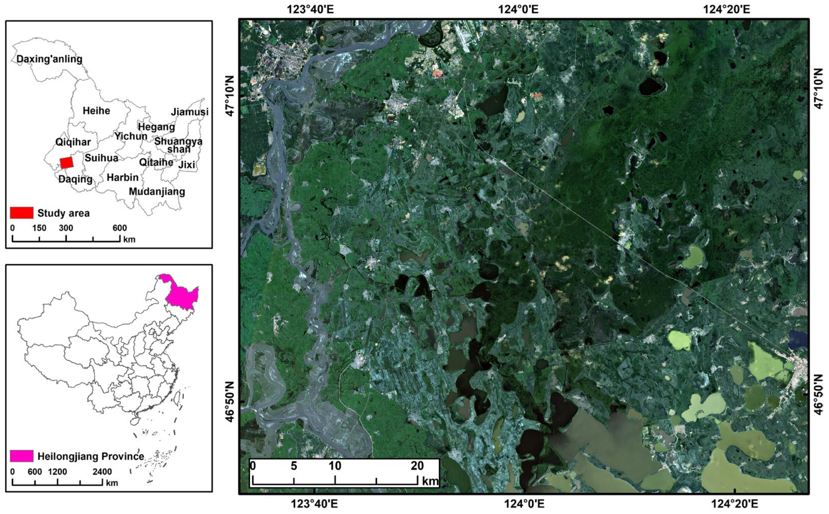
Figure 1. The geographical location of the study area.
Water 17 02877 g001
Figure 2. The statistical plots of spectral and microwave variables.
Water 17 02877 g002
Figure 3. The statistical plots of index variables.
Water 17 02877 g003
Figure 4. The statistical plots of geometry variables.
Water 17 02877 g004
Figure 5. The statistical plots of texture variables.
Water 17 02877 g005
Figure 6. The flow chart of the dynamic hybrid method for wetland mapping.
Water 17 02877 g006
Figure 7. Feature ranking and cross-validation accuracy of models based on ReliefF method. (a) Feature ranking; (b) Cross-validation accuracy of RF, XGBoost, and LightGBM models. The pink line represents the accuracy where the number of features is 23.
Water 17 02877 g007
Figure 8. Hyperparameter tuning using grid search, random search, and Bayesian search. (ae) represent the number of individual CARTs (n_estimators), learning rate of the boosting ensemble methods (learning_rate), the maximum depth of the trees (max_depth), the minimum number of samples at a leaf node (min_data_in_leaf), and the minimum sum of weights in a child (min_child_weight), respectively. (f) represents the classification accuracy of grid search (GS), random search (RS), and Bayesian optimization (BS) method in optimizing RF, XGBoost, and LightGBM models.
Water 17 02877 g008
Figure 9. Cross-validation accuracy of dynamic hybrid methods based on different ensemble models with RFE-selected features using importance metrics from ReliefF, SHAP, tree-based, and permutation methods. (a) Random forest method; (b) XGBoost method; (c) LightGBM method.
Water 17 02877 g009
Figure 10. Cross-validation accuracy of RF, XGBoost, and LightGBM models with RFE feature selection based on SHAP importance. The blue, red, and gray dashed lines in panel (a) indicate the optimal number of features. A–E represent the parameters ‘n_estimators’, ‘max_depth’, ‘learning_rate’, ‘min_data_in_leaf’, and ‘min_child_weight’, respectively. (b) represents the variables selected for the RF model; (c) represents the variables selected for the XGBoost model; (d) represents the variables selected for the LightGBM model.
Water 17 02877 g010
Figure 11. Confusion matrix for pixel-based and object-based RF, XGBoost, and LightGBM classification. C1 to C9 are the class codes representing barren land, built-up area, dryland, flooded land, grassland, marsh, paddy field, tree cover, surface water, respectively. (ac) represent the confusion matrix of objected-based RF, XGBoost, and LightGBM classification, respectively; (df) represent the confusion matrix of pixel-based RF, XGBoost, and LightGBM classification, respectively.
Water 17 02877 g011
Figure 12. Classification maps generated by the pixel-based and object-based RF, XGBoost, and LightGBM models. (ac) represent the classification maps of objected-based RF, XGBoost, and LightGBM models, respectively; (df) represent the classification maps of pixel-based RF, XGBoost, and LightGBM models, respectively.
Water 17 02877 g012
Figure 13. Mean absolute SHAP values for each feature across different classes in the LightGBM model.
Water 17 02877 g013
Figure 14. Evaluation of the overall impact of features on the LightGBM model’s classification results based on SHAP values.
Water 17 02877 g014
Figure 15. Evaluation of the interactive impact of features on the LightGBM model’s classification results based on SHAP values.
Water 17 02877 g015
Table 1. List of the calculation formulas for different indices using Sentinel-1 and Sentinel-2 images.
IndexFormulaReferences
NDVI ( NIR Red ) / ( NIR + Red ) [78]
NDVI-RE1 ( NIR RE 1 ) / ( NIR + RE 1 )
NDVI-RE2 ( NIR RE 2 ) / ( NIR + RE 2 )
NDVI-RE3 ( NIR RE 3 ) / ( NIR + RE 3 )
NDVI-RE4 ( NIR RE 4 ) / ( NIR + RE 4 )
MNDWI ( Green SWIR 1 ) / ( Green + SWIR 1 ) [79]
SAVI 1.5 × ( NIR Red ) / ( NIR + Red + 0.5 ) [80]
DVI NIR Red [81]
GCVI ( NIR / Green ) 1 [82]
RVI NIR / Red [83]
LSWI ( NIR SWIR 1 ) / ( NIR + SWIR 1 ) [84]
EVI 2.5 × ( NIR Red ) / ( NIR + 6 × Red 7.5 × Blue + 1 ) [85]
S2REP 705 + 35 × ( ( ( NIR + Red ) / 2 ) RE 1 ) / ( RE 2 RE 1 ) [86]
RRI V V / V H [87]
RFDI ( VV VH ) / ( VV + VH ) [88]
Gray ( 0 . 3 × NIR ) + ( 0 . 59 × Red ) + ( 0 . 11 × Green ) [76]
Table 2. List of crucial hyperparameter spaces for Bayesian optimization in RF, XGBoost, and LightGBM models.
Machine Learning ModelsHyperparametersSearch RangeStep
RFn_estimators[100, 2100]100
max_depth[2, 22]2
min_samples_leaf[5, 55]5
XGBoostn_estimators[100, 2100]100
learning_rate[0.1, 0.3, 0.5, 0.01, 0.03, 0.05]-
max_depth[2, 22]2
min_child_weight[5, 55]5
LightGBMn_estimators[100, 2100]100
learning_rate[0.1, 0.3, 0.5, 0.01, 0.03, 0.05]-
max_depth[2, 22]2
min_data_in_leaf[5, 55]5
Table 3. Computation time of different methods based on non-feature selection and feature selection. (Time unit: hour).
ModelWithout Feature SelectionFeature Selection
ReliefFOptimization MethodReliefFTreePermutationSHAPOptimization Method
Random Forest3.628Grid Search1.2081.3061.1711.237Bayesian Search
XGBoost4.3711.1181.4081.2141.244
LightGBM2.1720.9430.8800.9520.904
Disclaimer/Publisher’s Note: The statements, opinions and data contained in all publications are solely those of the individual author(s) and contributor(s) and not of MDPI and/or the editor(s). MDPI and/or the editor(s) disclaim responsibility for any injury to people or property resulting from any ideas, methods, instructions or products referred to in the content.