Article

Bayesian Analysis of Stormwater Pump Failures and Flood Inundation Extents

1
Research Institute of Water and Environment, University of Siegen, Paul-Bonatz-Strasse 9-11, 57076 Siegen, Germany
2
Emschergenossenschaft und Lippeverband, 45128 Essen, Germany
*
Author to whom correspondence should be addressed.
Water 2025, 17(19), 2876; https://doi.org/10.3390/w17192876
Submission received: 30 July 2025 / Revised: 28 September 2025 / Accepted: 29 September 2025 / Published: 2 October 2025
(This article belongs to the Section Hydrology)

Abstract

Former coal mining in the Ruhr area of North Rhine-Westphalia, Germany, leads to significant challenges in flood management due to drainless sinks in urban areas caused by ground depression. Consequently, pumping stations have been constructed to enable the drainage of incoming river discharge, preventing overland flooding. However, in the event of the failure of pumping stations, these areas are exposed to a higher flood risk. To address this issue, a methodology has been developed to assess the probability of pumping failures by identifying the most significant failure mechanisms and integrating them into a Bayesian network. To evaluate the impact on the flood inundation probability, a new approach is applied that defines pump failure scenarios depending on available pump discharge capacity and integrates them into a flood inundation probability map. The result is a method to estimate the flood inundation probability stemming from pumping failure, which allows the integration of internal failure mechanisms (e.g., technical or electronic failure) as well as external failure mechanisms (e.g., sedimentation or heavy rainfall). Therefore, authorities can assess the most probable pumping failures and their impact on flood risk management strategies.

1. Introduction

The Emscher/Lippe region is an area of 4145 km2, characterized by former coal mining, which has resulted in drainless sinks known as polders. These polders account for 20% of the total area and are home to 341,000 people [1,2,3]. These are areas where water from rainfall and watercourses accumulates and causes major flooding, including upstream areas that are flooded due to backwater. Therefore, pumping stations have been constructed to artificially drain the amount of incoming water [3]. As with other hydraulic structures, pumping stations are susceptible to failure due to a variety of issues, which are associated with their reliability [4]. Reliability, therefore, is defined as the probability that a hydraulic structure will perform its required function under specific conditions [5]. This poses a high risk, particularly in combination with heavy rainfall events, whose frequency and intensity are increasing due to climate change [6]. Depending on the current internal (pump-specific) and external (floods, severe weather) conditions, failure of some or all the pumps inside a pumping station may occur at any time. These alternative scenarios of pumping failure change the risk of flooding of the protected area. Therefore, authorities require methods to quantify the risk accounting for failure in order to better estimate and manage the risk of flooding to the population in these areas. Estimating the pumping station failures and the resulting probability of the flood inundation is the aim of this study.
For this purpose, probabilistic approaches for reliability analysis can be applied to quantify the probability of pump failure, taking into account the various types of pumping failure mechanisms. In urban drainage modelling, several studies exist assessing the failure probability of hydraulic structures in sewage networks [7,8,9] or protective structures such as levees and dikes [10,11]. For this purpose, probabilistic approaches such as Monte Carlo simulation, fault tree analysis, Bayesian networks (BN), and artificial neural networks are applied. In order to evaluate time-dependent failures, reliability analyses (e.g., Weibull analysis) of the service life of components (e.g., electrical components) are used by assigning a statistical distribution to the data [12]. Cousineau [13] considers up to three parameters in the reliability equations, which describe the failure rate (shape parameter), characteristic in lifetime (scale parameter), and a minimum life threshold (location parameter). Rizwan et al. [14] use a Semi-Markov model for reliability analysis of a pump system consisting of two pumps to obtain the mean time to failure. This method is based on the discrete state of the system, considering the likelihood of moving from one state to another (Transition probabilities) and the amount of time a system remains in a given state (Sojourn Time Distribution) [15]. The advances in machine learning (ML) in recent years have also led to new potential in water pump failure prediction using artificial neural networks (ANN) [16] and supervised ML techniques like multiple regression and decision tree cart [16,17]. Bayesian networks represent a further approach to determining the risk of failure by considering the interdependency of different failure mechanisms based on the chain rule and Bayes’ theorem [18]. This approach is often combined with Fault Tree Analyses or Monte-Carlo simulations, which are then used to define the failure causality (Fault Tree diagram) and to define the failure probability by applying a large number of numerical simulations (Monte Carlo Simulations) [19]. Another study of Veldhuis et al. [20] combine a reliability analysis using a probabilistic fault tree analysis with the assessment of urban flood probability, taking into account different failure mechanisms in a sewer network. Such approaches are also applied in combination for the assessment of pump failure. Bi et al. [21] use a Fault Tree analysis (FTA) based on a Tagaki and Sugeno model (T-S Fuzzy Fault Tree) [22,23] and combined it with a BN to apply a fault diagnosis of pumping units, focusing on the rotor of a pump. Another study developed a new method using various Weibull distribution functions for predicting the failure of de-watering pumps in deep-level mines, which pump water from the underground to the surface [24]. Bold et al. [25] investigated a method to determine the failure probability of a pumping station using a fault tree analysis. As a result, five independent failure mechanisms were determined that caused a total failure of the complete pumping station. The occurrence probability was obtained based on operation data, generic data, and an investigation for the pumping station’s supply security. The study examined pump station failure but did not consider dependencies between different failure mechanisms, nor the impact of individual pump failures on flooding. Therefore, a method is required that determines the failure probability of each pump in a pumping system individually and furthermore assesses the different impacts on flooding and its uncertainty.
Uncertainty assessment became a crucial part in flood modeling to obtain reliable results and is generally applied in risk assessment and flood management [16,26]. The sources of uncertainties in estimating flood inundation extents are manifold [27] and can be distinguished into two basic types, natural and epistemic uncertainties. Natural uncertainty reflects the variability of the stochastic process itself, while epistemic uncertainty derives from limited knowledge about the process [28]. Depending on the examined source of uncertainty, several approaches exist for quantification. In flood modeling, sensitive analyses are commonly used for identifying variables or parameters with the greatest influence on the uncertainty in flood prediction [29,30]. To estimate the impact of uncertainties on the outcomes, Monte Carlo-based frameworks represent one of the most common probabilistic approaches for uncertainty assessment [31,32,33]. Monte Carlo simulations derive the flood probability by producing a distribution of outcomes, investigating different uncertainties. In this framework, the application of generalized likelihood uncertainty estimation (GLUE) was developed to represent prediction uncertainties using a Bayesian Monte Carlo method, including likelihood weights based on observations [34,35]. To visualize and represent the obtained probabilities, probabilistic flood maps (PFM) are used to spatially map the probability of flooding. For instance, Quintana-Romero and Leandro [36] use a PFM to include uncertainties in flood extent resulting from multiple model structures, considering the interaction of the sewer network and overland flow. Alfonso et al. [37,38] quantify the uncertainties in flood extent occurring from land use changes and different operations of hydraulic structures. Moreover, PFMs are also applicable to reflect uncertainties of several input parameters, as in the study of Stephens and Bledsoe [39], who consider uncertainties from varying discharge, friction parameter, and channel change simultaneously. Domeneghetti et al. [40] demonstrate that PFMs can also be applied for the failure of flood protection measures using the technique to derive a PFM for dike failure.
Pumping stations consist of several pumps that run individually, depending on the current discharge or water level. Consequently, pumps can operate either independently or collectively. In order to quantify the failure probability of a pumping station, the failure probability of each pump must be derived individually. If a pump is independent, failure would only reduce the total pumping station discharge capacity, rather than causing total failure of the pumping station. Consequently, the impact on flooding varies depending on which pump fails. To our knowledge, there is no probabilistic framework for assessing the impact of individual failures of stormwater pumps on flood extent. Therefore, this article aims to develop a probabilistic approach, which is able to derive the failure probability of each pump in a pumping system individually, allowing an assessment of likely failure scenarios and their specific impact on expected flood extent. Against this background, this paper introduces a novel approach that determines the occurrence probability of failure scenarios based on the residual pumping discharge capacity of stormwater pump stations and translates the failure probabilities into a probabilistic flood map for flood risk assessment.

2. Materials and Methods

2.1. Case Study

The study area is located in Dorsten, in the German federal state of North Rhine-Westphalia, and has a total population of around 74,515. The detailed study area (see Figure 1) covers 5.47 km2 and is located inside a catchment of 171.20 km2 [41]. There are two main inflows, the rivers Hammbach and Wienbach, which merge within the considered study area. Moreover, a third, smaller inflow to the Hammbach exists upstream of the confluence of the two main rivers. Due to a drainless sink caused by former coal mining, a pumping station is required in the south, only a short distance after the confluence of the two main rivers (Figure 1).
Without the pumping station, the natural flow of the river would be impeded, resulting in flooding of the city of Dorsten. Therefore, the pumping station continuously pumps the incoming discharge westward to a river section of the Hammbach with natural flow to bypass the polder area. From there, the river flows naturally to the Lippe River downstream. A total discharge capacity of 15.5 m3/s is available from the four stormwater pumps. An overview of the existing stormwater pumps and their discharge capacity is given in Table 1.

2.2. Framework for Pump Failure Assessment

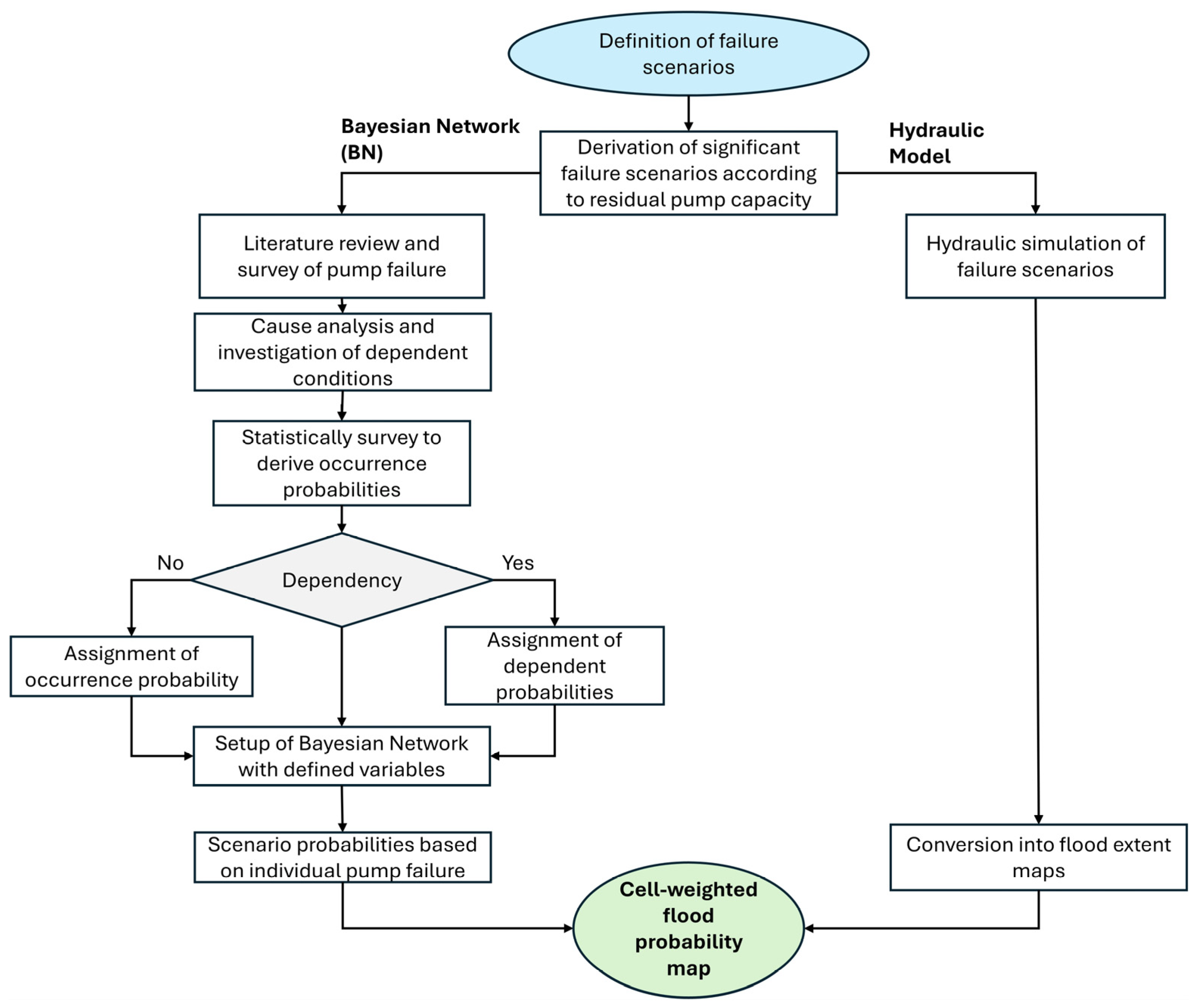
In order to assess the probability of flooding in relation to the current pump status, a workflow consisting of three main steps is required. First, failure scenarios are defined according to the number of pumps in a pumping station. Second, a Bayesian model is set up to derive the failure probability of each pump. Finally, corresponding flood events are simulated to assess the impact of pump failures on flood characteristics. Based on the outcomes, a flood probability map can be generated that allows an assessment of expected flooding considering the current conditions affecting the operation of a pumping station. An overview of the workflow is described in Figure 2.
The first step of the developed approach is to define the possible failure scenarios depending on the number of existing pumps in a pumping station. Because this could result in an excessive number of failure scenarios, the analysis was limited to the significant scenarios determined by the total residual pump capacity. The next step can be split into the setup of the BN and the hydraulic model. The BN aims to derive the failure probability of each pump in a pumping station individually. Therefore, pump failure mechanisms and their causality are derived from a literature review and a survey of pump operators. Based on the results, the occurrence probabilities of the determined failure mechanisms are statistically derived. If the variables are independent, the probability is assigned directly to the variable. In case of dependency on other variables, the dependent probability is determined first and assigned to the considered variable. To set up the BN, all derived variables are integrated into a network, including their interdependence and the determined probabilities. Based on the individual pump failure probabilities, the total probability of the defined failure scenarios can be derived. To integrate the probabilities into a flood map, the hydraulic model is used to simulate the corresponding inundations. The generated flood maps, consisting of the maximum water depth, are converted into a flood extent map, which can then be used to derive a cell-weighted flood probability map by integrating the probability of all scenarios.

2.3. Framework to Determine Pumping Failure Scenarios

Pumping stations are designed to drain large volumes of water. Therefore, several pumps are required, each with different pumping characteristics. This not only provides the system with increased capacity at peak times, but also redundancy in the system so that the pumps can operate at an alternative rhythm. To quantify the number of failure scenarios, two equations are developed to describe the number of potential failure scenarios and the significant number of failure scenarios based on the pumping discharge capacity. The number of potential failure scenarios can be described by the following equation:
F S = 2 n 1
where n describes the number of pumps. Constant 2 is derived from the number of possible states (on/off), and constant 1 describes the scenario in which all pumps are running. This state is subtracted to obtain the total number of failure scenarios (FS). For pumping stations consisting of a large number of pumps, a significant number of failure scenarios need to be considered. To reduce the number of scenarios, this study implements a concept that defines failure scenarios based on total pump capacity. This allows us to set the focus on scenarios resulting in the same flood inundation extent. Thus, Equation (1) is modified to the following:
F S =   2 n ( 1 + i k ( F S P C e q u a l , i 1 ) )
The total number of failure scenarios is now calculated by subtracting the scenario in which no pump failure occurs (represented as 1), in addition to the sum of the number of failure scenarios with the same pump discharge capacity (FSPCequal,i). Where i describes the number of failure scenarios with a total-pumping discharge capacity of i, and k describes the number of existing scenarios with an equal discharge capacity.

2.4. Pump Failure Mechanisms

To identify critical and significant failure mechanisms for stormwater pump stations, a set up of possible pump failures is derived from literature and reasoned relations based on logical interdependencies. The setup is verified by pump operators. Like every other type of technical device, technical failures depend on the correct operation of technical components. Technical failures can be divided into mechanical and electronic failures. However, external factors can also disturb the pump machine and lead to failure. Through literature review and information from pump operators, several failure mechanisms have been identified that can occur individually or simultaneously. Each mechanism is influenced by external conditions, which are partially interdependent. The failure mechanisms are presented below:
  • Power failure (external): Power failures are more likely to occur during thunderstorms and are strongly influenced by the type of power supply. Pumping stations typically include redundancy. The more redundancies, the less likely a total power failure is. The existence of an emergency generator that can supply the pumping station with electricity in case of an emergency reduces the likelihood of failure [25].
  • Failure due to flooding (external): There is a significant increase in the likelihood of damage or complete destruction of the technical components of the pumping station in the event of flooding. This is primarily influenced by the type of structure (e.g., waterproof design) and the incoming discharge [25,42].
  • Failure due to sediments (external): A riverbed is characterized by the transport of sediments. During periods of high discharge, more sediments are carried into the river and transported downstream. The more sediments are present, the greater the risk that they enter the pump and cause a blockage. This scenario is primarily affected by the amount of incoming discharge and the presence of a sediment protection system, such as nozzles, at the entrance to the pumping station.
  • Material failure (internal): Mechanical disturbances are a main cause of pump failure. Consequently, a pump may fail during regular operation, causing an abrupt change in available discharge capacity. The likelihood of mechanical failure depends on the pump’s age and condition, both of which can be improved through regular maintenance [16,43,44].
  • Electronic failure (internal): In addition to the mechanical components, pumping stations consist of a wide range of electronic components that have a limited lifetime and are therefore at risk of malfunctioning. These components control the operation of a pump with sensors and transmission of information, and thus can lead, in case of malfunction, to complete failure. As with mechanical components, maintenance services can prevent malfunctions and reduce the risk of pump failure [45].
  • Pump start disturbance (external): Pumps are activated when a certain discharge or water level threshold is exceeded. In the event of a high discharge, sediments can enter the pump and hinder the starting process. For example, after past flood events, large quantities of sediments may be carried into the pump inlets that have been turned off. This may block the rotor blades and prevent the pump from starting when needed. Flushing nozzles can reduce the risk of pumps becoming blocked by cleaning out sediments.

2.5. Pump Failure Mechanisms and Failure Probability

As technical systems, pumps are limited in terms of durability due to abrasion and other internal failure mechanisms [43]. However, external failure mechanisms, such as floods, can also affect the operation of pump systems, increasing the risk of failure [42]. In order to derive a failure probability, the significant failure mechanisms must be defined first. This is achieved through a review of existing literature and a survey of local pump operators. The survey is conducted based on the pre-determined most common pump failure mechanisms identified during the literature review and pump operator survey, to determine empirical data, covering the circumstances and frequency of past pumping failure events. Subsequently, the required empirical probability of an event A can be derived from the observed data by the following expression [46]:
P A = n ( A ) n
where n represents the total number of observations and n(A) the number of observations when event A occurred. The dependent probabilities of event B from event A are calculated by:
P B A = P ( A B ) P ( A )
whereas P ( A B ) represents the probability of the occurrence of events A and B [47].

2.6. Bayesian Network for Individual Pump Failure Probability

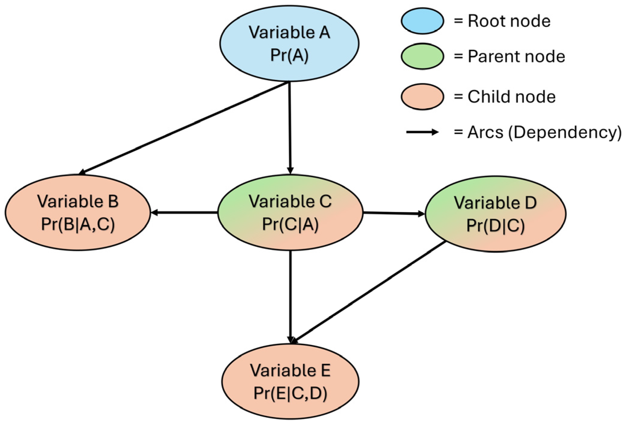
The identified pumping failure mechanisms are subsequently integrated into a BN, which enables the inclusion of various mechanisms contributing to pump failure. Furthermore, the interdependencies of those mechanisms are considered. Bayesian networks are probabilistic models that are commonly used for systems reliability analysis, safety analysis, and risk assessment [48]. A BN is a directed acyclic graph (DAG) characterized by qualitative as well as quantitative components, which aims to graphically illustrate the conditional dependencies between variables and to derive their probabilities. The variables (i.e., pump failure mechanisms) in a BN are represented as nodes and their dependencies as arcs. Depending on their dependencies, the nodes can be classified into three different types. Initial and independent variables are called superior nodes and are characterized by not having any subordinate nodes. These nodes are also called root nodes. Nodes, which affect one or several subnodes, are called parent nodes. The dependent nodes affected by parent nodes are called child nodes. Each node is assigned a conditional probability table, which considers the dependencies on the parent nodes [46]. An example of a simple network is shown in Figure 3.
The BN enables the posterior probability of unknown variables to be estimated by considering given variables [48]. It is based on the assumption that all root nodes are conditionally independent. The other nodes are conditionally dependent only on their direct prior nodes, i.e., parent nodes. The joint probability distribution is calculated according to the conditional independence and the chain rule. This relationship can be expressed as follows:
P X 1 , X 2 , , X n = i = 1 n   P X i P a X i
whereas Xn represents the variables and Pa(Xi) is the parent of the considered variable Xi [49]. The main application of BN constitutes the update of prior occurrence probability when new information (i.e., evidence) becomes available. Therefore, given occurrences of variables can be integrated into the network, allowing the posterior probability of dependent variables to be updated. This calculation is described by the Bayes Theorem [18]:
P r ( A B ) = P r ( B A ) P r ( A ) P r ( B )
where Pr(A/B) is the dependent probability of A given B, Pr(B/A) is the dependent probability of B given A. Pr(A) and Pr(B) are the prior probabilities of events A and B (A priori probability). Thus, a BN can be used to consider initial states and boundary conditions and to derive the failure probability of each pump individually. Subsequently, the occurrence probability of every failure scenario S can be derived by the chain rule [18]:
P r s 1 s 2 , , s n = i = 1 n   p i s i 1 p i 1 s i
where si is the state of each pump i with si {0,1}, whereas 1 = failed and 0 =running, pi is the failure probability of each pump i and n is the number of pumps. The final probability considering all the failure scenarios (with corresponding reduced pump discharge capacity) can be derived by the sum of individual probabilities:
P r F S 1 F S 2 , , F S n = P r ( s P C e q u a l )
where SPCequal represents the scenarios with the same pump discharge capacity.

2.7. Dual-Drainage 1D/2D Model

Pump failures lead to a reduction in the total-pumping discharge capacity, which has a significant impact on flooding if the incoming flow exceeds the available capacity. The flood inundation resulting from each failure scenario is obtained by integrating the pump state into a numerical model. A literature review comparing different types of urban flood models by Bulti and Abebe [50] demonstrates that 1D/2D coupled drainage models represent the most accurate model type for urban flood modeling. Therefore, several coupled 1D/2D models have been developed in recent years to properly represent urban drainage features, as well as the overland flow [51,52,53]. In this study, the 1D/2D coupled model developed by Leandro and Martins [36,52] is set up using the storm sewer model SWMM 5.1 and the 2D overland model P-DWave. P-DWave 2D is a parallelized diffuse wave model, which uses a simplified momentum equation of the 2D shallow water equation by considering only the pressure and friction term described by:
h t + ( u h ) = S
g ( h + z ) = g S f
where g = acceleration due to gravity, z = bed elevation, h = water depth, u = depth average flow velocity vector, S = sink/source term and Sf = bed friction vector [Sfx Sfy]T. The bed friction term is approximated by Manning’s formula [54]. SWMM is a 1D stormwater management model for urban runoff simulations based on the St. Venant equations, as well as for modeling drainage systems in urban areas [55]. Thereby, the 1D model represents the riverbed and sewer system, including the pumps, while the 2D model represents the overland flow resulting from pluvial and fluvial flooding. The coupling of these two models enables an accurate representation of the sewer system and pumping station, as well as surface runoff, and allows a more realistic calculation of urban flooding.
To achieve a good compromise between calculation time and adequate representation of the terrain, a resolution of 5 m is chosen. Buildings are represented as blocking elements of the flow by raising the terrain by 5 m. The two models communicate through exchange nodes, considering the hydraulic head difference between the 1D and 2D models. The discharge exchange is calculated by a weir or an orifice equation, depending on surcharge or drainage conditions [52]. Further details on the 1D/2D model can be found in [52,54].

2.8. Flood Inundation Probability Map

The flood inundation probability considering pump failures is quantified by a likelihood weight-based approach in the form of a flood probability map. To derive a flood probability map from inundation maps, each cell must be assigned a wet or dry state. Since we consider fluvial and pluvial flooding, each cell in the case study receives water. Therefore, a flooding threshold is required to prevent every cell from being assigned as wet. This threshold is set at 0.1 m, representing a water depth at which a moderate flood hazard is expected [56]. The likelihood weight is defined as the likelihood of the corresponding failure scenario obtained in Section 2.3. Subsequently, the average weighted flood state Ci, considering all scenarios, is determined as follows [57]:
C i = Σ k L k w k i Σ k L k   × 100
where w is the state of the considered cell i based on the set threshold (wet = 1, dry = 0), L is the likelihood and k is the corresponding scenario. This calculation is performed for each cell in the case study. If cells are assigned a 100% or 0% probability, this means there is no uncertainty about whether those cells are wet or dry. A value of Ci of 20% indicates a 20% probability that the cell is wet.

3. Results

Due to data privacy protection, the presented probabilities and derived results in this section constitute fictional data and do not represent the real data for the case study. It is noted that the real data are characterized by significantly lower failure probabilities.

3.1. Pump Failure Scenarios

In order to assign a probability of pump failure to the scenarios, each failure scenario must first be defined. Each pump in a pumping system can fail independently leading to different failure scenarios. Applying the formula of Equation (1) the existence of four pumps in Table 1 leads to a total of 15 failure scenarios, which are determined by considering all possible combinations of pump failures. An overview is given in Table 2.
Table 2 shows that several scenarios have the same total-pumping discharge capacity (PC). Since these scenarios result in the same flood inundation, the number of relevant scenarios can be reduced by considering only the total capacity instead of individual pumps. Thus, the number of scenarios considered is reduced from 15 to 7 resulting from the same pump capacity of pump 2–4. The remaining failure scenarios are illustrated in Table 3.
These failure scenarios, as well as the scenario of no failure, represent the final scenarios, which are considered for the simulations by the numerical model and for calculating the probability of each scenario.

3.2. Pump Failure Assessment

3.2.1. Pump Failure Mechanisms—Survey Results

Based on the survey and interviews of pump operators, the pump failure mechanisms in Section 2.4 can significantly affect the pump’s operating. Therefore, six causes of failure and the described interdependencies are considered in the further steps of probability determination, including power failure, failure due to flooding, failure due to sediments, material failure, electronic failure, and pump start disturbance. Moreover, the survey identified some failure mechanisms that have common triggering preconditions. For example, discharge has a direct impact on the water entering a pumping station and on the amount of sediment in rivers, and can therefore lead to two possible pump failure mechanisms. Regular maintenance, on the other hand, is important to prevent material as well as electronic failure of pumps.

3.2.2. Derivation of the Probability Distribution

To derive probabilities for implementation in a Bayesian network, a survey based on identified pump failure mechanisms is conducted and statistically evaluated. The survey’s structure is designed to empirically derive the probabilities of failure mechanisms, and a questionnaire of 17 questions regarding the occurrence of failures and their causality. The questionnaire covers information about existing pump-specific variables represented by the pumping station properties, containing age, electricity supply, construction type, protection measures, and maintenance interval. Furthermore, the survey provides conclusions about the frequency and circumstances of the determined pump failure mechanisms in Section 3.2.2. The empty questionnaire is provided in Supplementary Materials. The survey is distributed to the 10 available operators of large pumping stations in the Emscher/Lippe catchment area with comparable construction and conditions as the considered case study. Based on the results, the independent and dependent probabilities are derived by statistical evaluation based on Equations (3) and (4), which provide information on how often and in what circumstances pump failures occurred in the past. For the sake of illustration, sample data are shown for the availability of electricity supply in Table 4.
Table 4 illustrates an example of assigned probabilities to electricity availability. For instance, if severe weather occurs in combination with a single power supply, the probability of an available electricity supply is 92%, and 97% if a dual power supply exists.

3.2.3. Bayesian Network

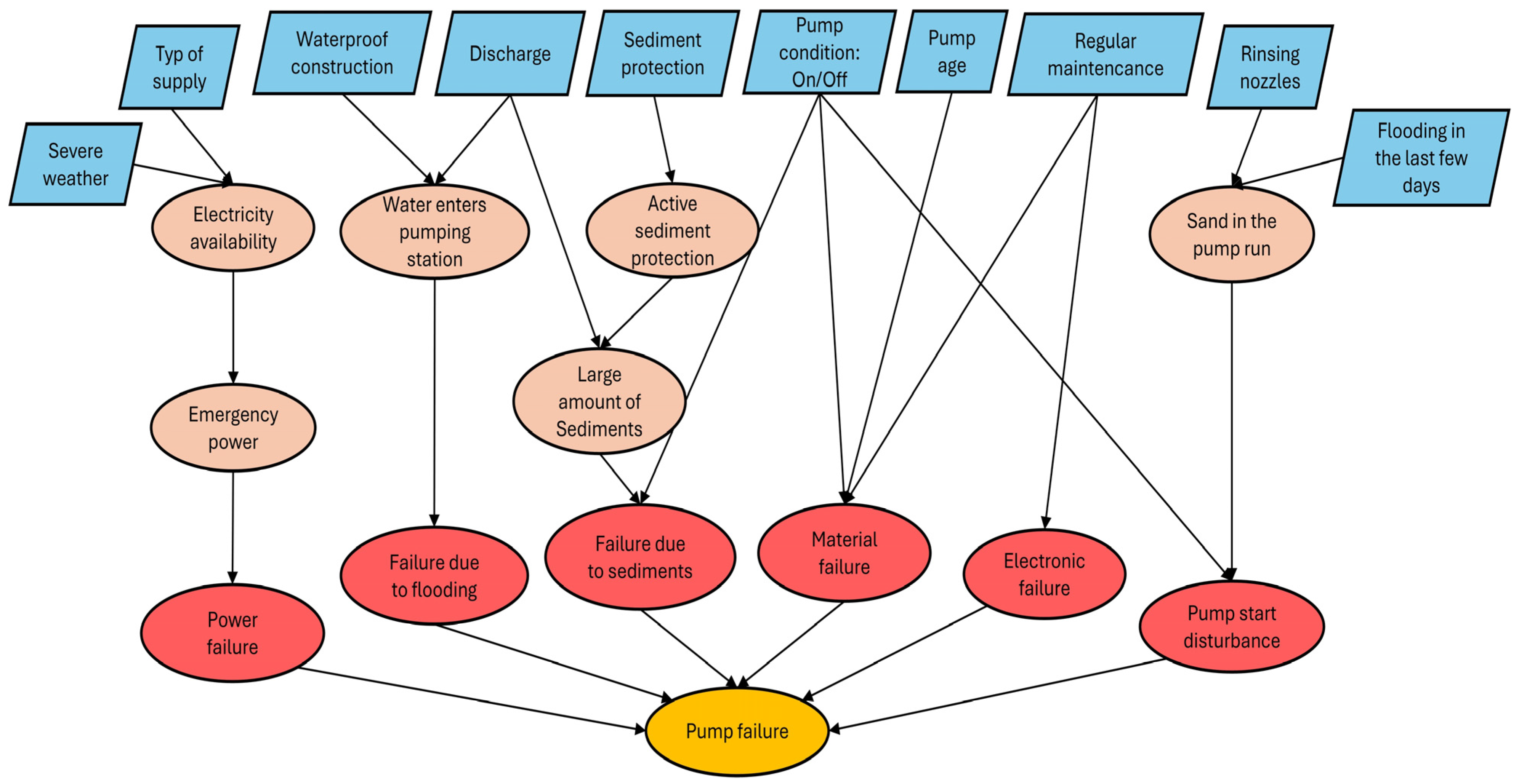
The pump failure mechanism and the derived probability distributions described in previous chapters are integrated into a Bayesian network. Therefore, the initial variables are defined as root nodes that set the initial state. These initial variables constitute the observed and given variables (a priori knowledge) and must be manually set before the network is started. Dependent variables are subsequently set based on the defined pump failure mechanism. The last child nodes represent the scenarios that lead to different types of failure, depending on their parent nodes. The resulting Bayesian network is shown in Figure 4.
The initial variables (blue nodes), such as the pump-specific properties (type of supply, pump age, and sediment protection), as well as the initial conditions (flooding, severe weather, and pump state), are set manually and are considered independent. Each dependent variable is defined by a conditional probability distribution that is directly affected by the root nodes. These dependencies are represented by the edges between the nodes in the network. Thus, one variable can have several parent nodes from which it depends. For instance, the availability of electricity is affected by the type of supply (e.g., single or double) and the occurrence of severe weather. Finally, the probability of a failure scenario (red nodes) and, consequently, the total failure probability of one pump is derived by applying the chain rule (Equation (5)). In the case of new information, the a priori knowledge of all variables can be updated, and a new probability distribution for each variable can be determined based on Bayes’ theorem (Equation (6)). To calculate the failure of each pump, this process can be iteratively repeated for each pump. Finally, the total failure probability of the pumping station can be derived from the failure probabilities of each pump using the chain rule.
As an example, this procedure is shown in the following for three different scenarios. The three scenarios differ depending on the internal and external influence factors: regular operation, flood scenario, and extreme scenario. The regular operation constitutes a general state with no extraordinary influence factors. The second scenario illustrates a flood scenario combined with severe weather. The extreme scenario represents a worst-case scenario combining the conditions of the flood scenario with flooding in the past, and without regular maintenance. For simplicity’s sake, it is assumed that each pump has the same conditions described above, except for age. An overview is provided in Table 5.
By assigning the a priori knowledge of Table 5 to the initial variable in the Bayesian network, the failure probability for each pump can be determined based on the derived probabilities in Section 3.2.2 and the chain rule (Equation (5)). The result is displayed in Table 6.
The constructed results demonstrate that failure during regular operation (i.e., normal conditions) is unlikely. The highest probability is 5% for the oldest running pump. In case of flooding, the failure probability increases from 5% up to 29% for pump 3. The highest failure probabilities for each pump are obtained in the extreme scenario, with the highest value of 78% for pump 3. Subsequently, the probabilities of each pump state (on and off) can be derived using the obtained failure probabilities. For the sake of illustration, further steps are only shown for the flood scenario, which is illustrated in more detail in Table 7.
The calculation of the occurrence probability for the failure scenarios in Table 2 is obtained using the derived probability in Table 7 and their multiplication based on the chain rule from Equation (5). The obtained probabilities are shown in Table 8.
As illustrated, each scenario is assigned a probability and a residual-pumping discharge capacity. Several scenarios result in the same total-pumping discharge capacity. These scenarios are characterized by the same impact on flooding and can therefore be considered as one failure scenario. To calculate the occurrence probability of this combined scenario, the probabilities of each individual scenario are aggregated. These scenarios represent the final scenarios considered for the flood inundation probability assessment. An overview is given in Table 9.

3.3. Flood Probability Map

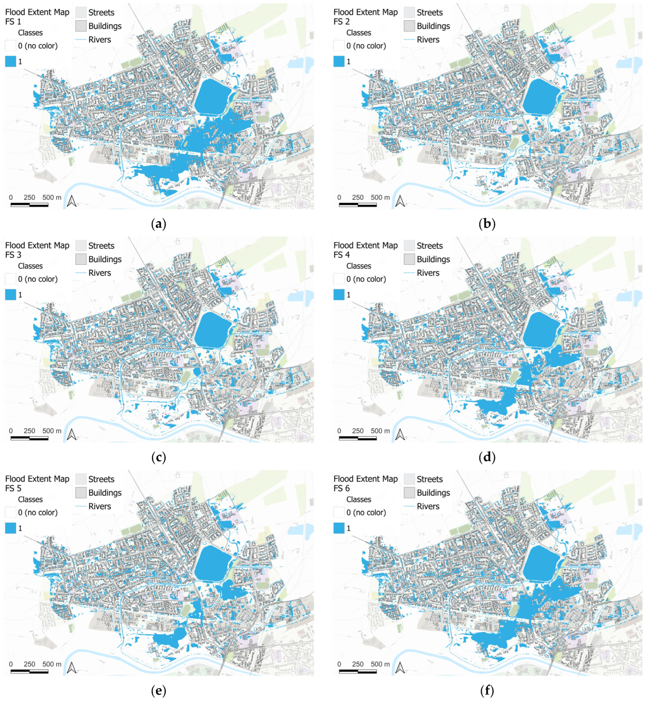
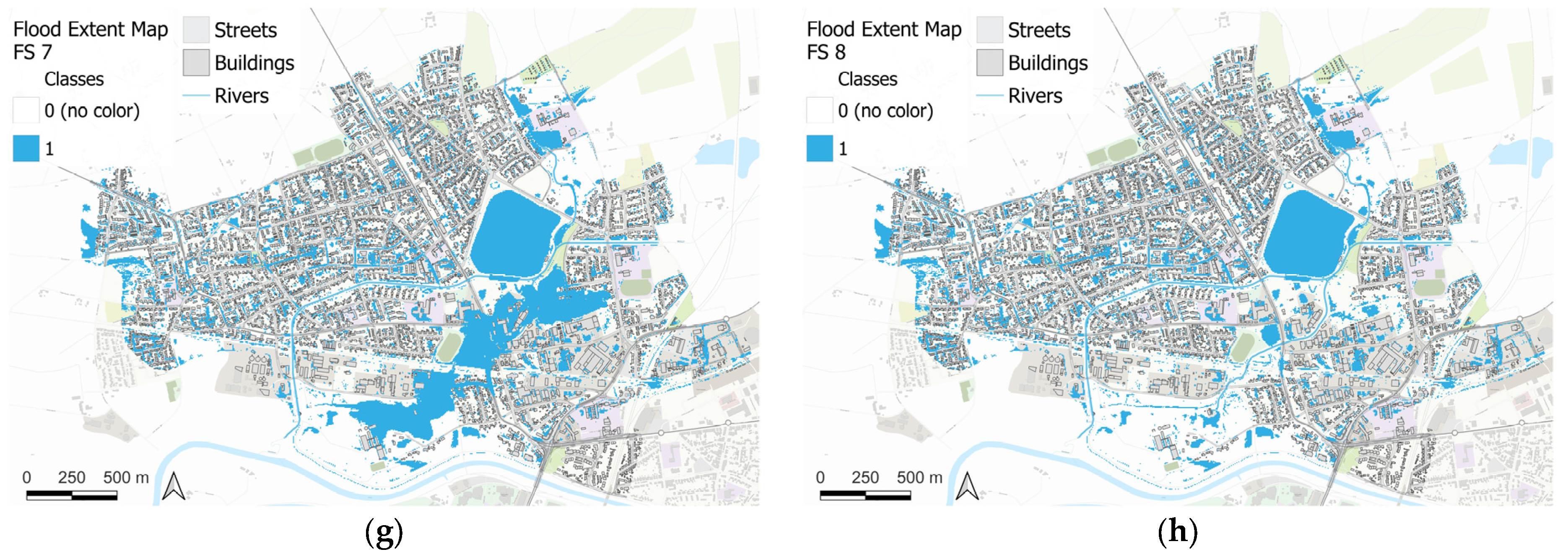
Each scenario is distinguished by a distinct flood inundation and assigned an individual probability. The initial step in assessing the flood inundation extent is to convert the inundations containing the maximum water depth of the corresponding failure scenarios in Table 9 to a flood extent map. This is achieved through the allocation of cells with a water depth greater than 0.1 m to a category of 1, while cells with lower water depths are designated as 0. In the following, an overview of the derived flood extent maps of all scenarios, including the scenario with no failure (scenario 8), is provided in Figure 5.
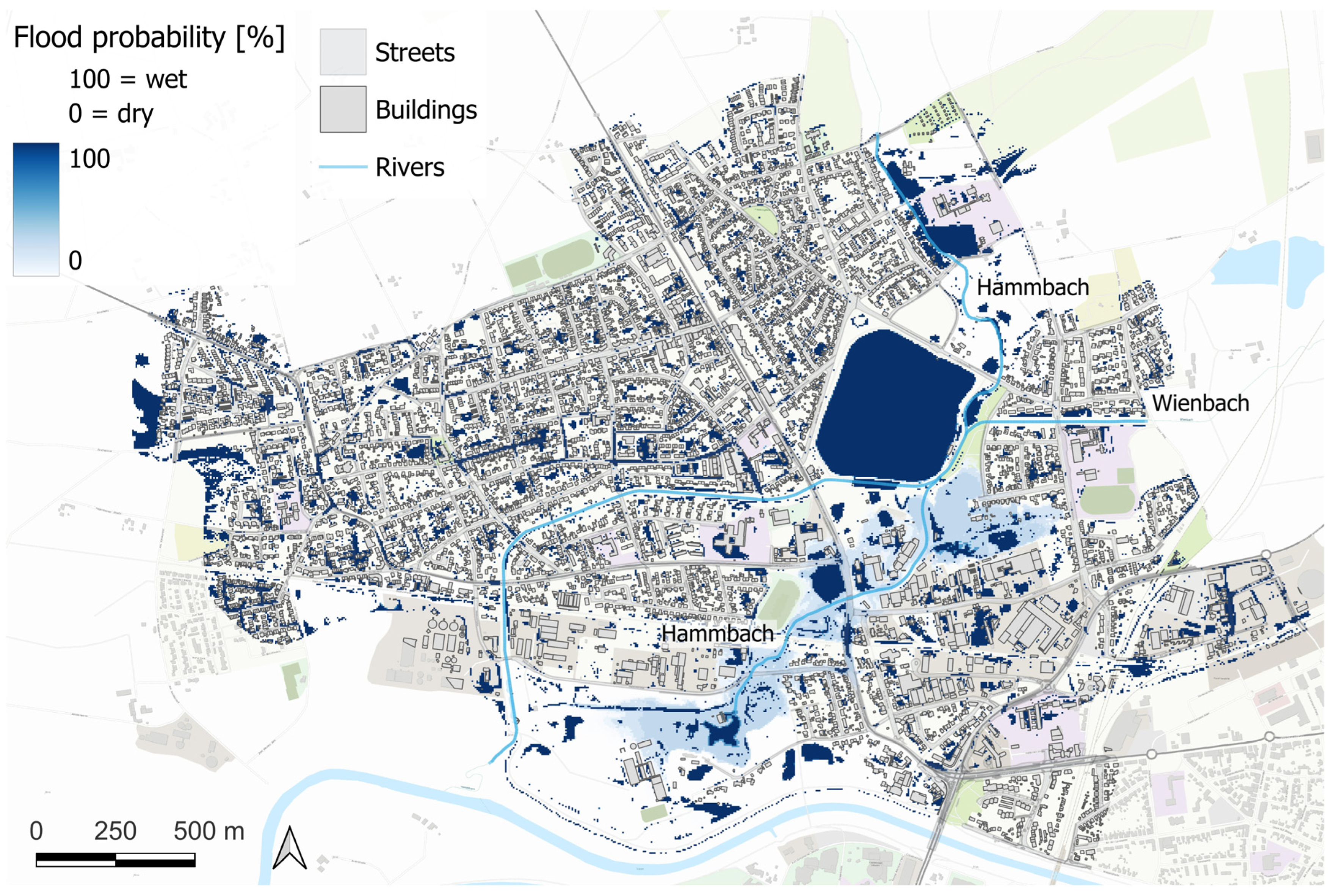
The created flood extent maps demonstrate a wide range of inundation extent, depending on the failure scenario considered. The flood extent maps show the differences in the extent of the simulated flooding, which are associated with a probability of occurrence. To quantify and visualize it in a descriptive form, the determined flood extent maps are summarized in a flood probability map. The varying probabilities presented in Table 9 illustrate the probability of being wet/dry resulting from pump failure. For Instance, Figure 6 shows one example of a flood inundation probability map obtained for a rainfall event with a 100-year return period, considering all failure scenarios investigated.
The flood inundation probability map is a representation of the likelihood of flooding in each cell for a given rainfall event, taking into account all potential failure scenarios as well as the scenario of no failure. The coloration of the map is intended to convey the relative likelihood of flooding in each area. The dark red regions indicate areas with the highest probability of flooding, while the light red regions indicate areas with a lower probability. The dark red areas, designated by 100%, represent areas that are wet in each considered scenario and are consequently not dependent on the pumping capacity. Cells assigned with values between 0 and 100% have a probability of being wet depending on the derived failure probabilities. Therefore, a value of 90% for example, can be interpreted as having a 90% probability of being wet for a rainfall event with 100-year return period. Cells with a probability between 0% and 100% are found in the area around the Hammbach after its confluence with the Wienbach, wherein the extent of fluvial flooding varies depending on the scenario of pump failure. Since the failure of the pumps is still unlikely for the considered flood scenario, the probability of large fluvial flooding is relatively low.

4. Discussion

4.1. Pump Failure Scenarios

The derived failure scenarios in Table 2 demonstrate the large number of scenarios that need to be considered for flood risk assessment. The focus on the available pumping discharge capacity enables the summary of events leading to the same flood extent and thus offers a more structured and clearer overview of the relevant scenarios, as seen in Table 3. The more structured overview of the significant scenarios allows an effective assessment of failure scenarios and reduces the effort for evaluation and generation of flood inundation extent maps and the corresponding flood probability map for one flood event. Since all possible flood scenarios are still considered, no compromises are required regarding accuracy and efficiency.

4.2. Pump Failure Assessment

4.2.1. Pump Failure Mechanisms

The determined failure mechanisms can be divided into external and internal factors. Internal factors are, for example, sediment protection, power supply, or age, and those can vary depending on the considered case study. External factors represent those that have a larger influence on the operation of the pumps and are not influenced by the pumping station itself. Such factors constitute, for example, the flooding event or weather severity that occur regardless of the type of pumping station but significantly affect the operation of the pump. The failure causalities represented by the derived failure mechanism are characterized by a complex interaction of several factors, which are specific to stormwater pumps. The interaction is characterized by the dependency between the failure mechanisms, as in the example of sedimentation and flooding. Blocking through sedimentation is directly influenced by the incoming discharge and the protection configuration of the pump. Moreover, the discharge has an additional impact on flooding, which can lead to water entering the pumping station and consequently to pump failure. This makes the representation of all failure mechanisms and their interdependency highly complex. It is noted that the defined failure mechanisms are specific to the case study and represent the main causality for failure of the pumping station being studied. For example, in the case of de-mining pumps in Jacobs et al. [24], thunderstorms had less impact on power failure. Also, the sewage pumps in Piri et al. [16] were neither impacted by flooding nor sedimentation of the river bed. Nevertheless, internal failures like mechanical or electrical failures constitute a universal failure mechanism of technical devices like pumps. The method is, in any case, transferable to other pumping stations. In that case, an additional field survey and literature review on the type of pumping station investigated is required.

4.2.2. Bayesian Network

The set-up of BN in Figure 4 demonstrates that its application enables an explicit representation of different defined failure mechanisms and their direct dependencies among each other, which lead to a pump failure. Accordingly, it clearly represents variables that have a direct influence on pump failure and facilitates a derivation of different causal scenarios (“what-if” scenarios). The derived pump failure mechanisms and their causalities are directly implemented into the network as variables. The representation as a direct acyclic graph makes the system transparent and more understandable for the applicator, allowing a more comprehensible assessment of interdependencies. As an example, the dependency of flooding as well as sedimentation on the incoming discharge, which both lead to pump failure independently, can be clearly represented. The individual properties of a pumping station, such as protection structures, age, or pump state, are set as initial variables and are not assigned by a probability table. This allows the integration of different pumping structures, which makes the system more transferable to other case studies. To cover a wider range of pumping stations, the network can be easily extended by additional properties like pump types or pump size, which may affect the durability of pumps.
The scenarios shown in Table 5 illustrate that the set-up BN can be applied to represent different scenarios, which cover different states of the variables and their impact on the operating pump. The ability to calculate the probability of pump failure in seconds makes the network highly suitable for sensitive analyses investigating the impact of different combinations of variables on the pump.
The derived failure probabilities in Table 6 illustrate that the influence of each variable has an individual impact on the pump failure and is strongly influenced by the other. For instance, severe weather combined with flooding does not lead to a significant risk of a pump failure. This is due to the protection measures implemented, such as waterproof construction, dual power supply, and regular maintenance in place. If these initial conditions are not present, the risk of pump failure increases significantly. That can be seen in the case of the extreme scenario. Other variables, such as age, have less impact on the pump operation if regular maintenance is carried out. This illustrates the importance of representing pump failure mechanisms and their dependencies to estimate the failure of pumps. Furthermore, BNs have the additional advantage that if additional failure mechanisms need to be implemented retrospectively, they are easily added. This adjustment can be performed by implementing new dependencies/variables derived from additional literature or field surveys. Since each variable holds its local conditional probability table, additional variables can be assigned new probabilities independently of the existing ones. This makes the developed network transferable to other pumping stations. Moreover, in case of data scarcity, the system benefits from the possibility of integrating expert knowledge or assumptions that enhance the system’s resilience and ensure permanent operability.
The derived probabilities of the different scenarios in Table 8 demonstrate that each scenario is assigned with an individual probability, even if the scenarios have the same total-pumping discharge capacity. The benefit of considering the total-pumping discharge capacity is seen in the subsequent step, when all scenarios are summarized and shown in Table 9. Thereby, the relevant scenarios can be reduced by more than half, leading to a more efficient management of data. The large range in the probabilities obtained for each scenario stresses the relevance of considering all scenarios and not only the scenario with the highest probability.

4.3. Flood Probability Map

The simulated inundations for different failure scenarios in Figure 5 illustrate the high variation in flood patterns resulting from missing pump discharge capacity. Clearly, the higher the number of pump failures, the larger the resulting flood inundation extent is. Since the simulations consider a 100-year return period of heavy rainfall over the entire catchment area, inundation occurs due to both fluvial and pluvial flooding. Pluvial flooding affects the entire study area and is uniformly distributed across the considered urban area. This type of flooding constitutes the main reason for flooding in scenarios 2, 3, and 8 and can be seen in all scenarios as it is independent of the pump discharge capacity. Fluvial flooding occurs when the river’s discharge capacity is exceeded and is primarily located near the river. The latter occurs when the residual-pumping discharge capacity is insufficient to pump the incoming river discharge. This results in backwater and an increase in water depth in the upstream regions. This is clearly evident in scenarios 1, 4, 5, 6, and 7. Thereby, fluvial flooding only occurs if the incoming discharge exceeds the residual-pumping discharge capacity, which can be seen in the additional flood extent comparing failure scenarios 2 and 5 with a respective residual-pumping discharge capacity of 11 m3/s and 9 m3/s.
Comparing the flood extent of the two most likely scenarios, 2 and 8 in Figure 5, no significant differences can be observed, since the incoming discharge does not exceed the residual-pumping discharge capacity. This changes when considering the flood extent of the third most likely scenario 4, with a significant occurrence probability of 12.3%, which is characterized by a large inundated area. These uncertainties in flood extent make it highly complex to assess the likelihood of the flood inundation pattern.
The integration of the obtained occurrence probabilities of each failure scenario into a flood probability map, as seen in Figure 6, allows a clearer overview of the uncertainties regarding pump failures and facilitates the interpretation of the existing flood probability resulting from a flood event. Considering the probability of inundation based on pump failure scenarios in the case study, the areas assigned a value of 1 or close to 1 constitute areas that are primarily a result of pluvial flooding (rainfall) and therefore not dependent on the pumping discharge capacity. Cells with an unclearly defined state, being wet or dry, are located in the area around the Hammbach after its confluence with the Wienbach, whereby the inundation extent of the fluvial flooding varies depending on the scenario of pump failure. Since the scenarios with failure of several pumps are assigned by smaller occurrence probabilities leading to larger inundations, the probability of large fluvial flooding is smaller. The conversion into a flood probability map has the advantage that it consolidates all information in a single map and explicitly illustrates the expected probability of occurrence, making it clear and easy to interpret. Since wet areas are assigned a 1, the corresponding probability can be directly derived from the resulting flood probability map. This makes it clear and structured for authorities and simplifies the decision-making for appropriate flood protection measures.

4.4. Limitations

We would like to note that this study focuses on technical errors and neglects human errors, which are more difficult to quantify. One reason for this is that access to such data is sensitive to operator information. In real applications, access to such information as well as likely pump failure mechanisms may be limited, incomplete, or simply not possible. Although the methodology can also be applied to other studies, the survey must be repeated. The results of the survey are only representative of the conditions in our study and cannot be generalized to other case studies. Ideally, the survey should be extended to the entire federal state of North Rhine-Westphalia in order to increase its representativeness and the generalizability of the flood maps produced for other locations. Furthermore, it is very complex to capture all factors of failure mechanisms, but the methodology can easily be expanded by including other mechanisms and more dependencies. Together with more extensive surveys, these would have an impact on the results of the flood probability maps.

5. Conclusions

This paper develops a novel approach for pump failure assessment that predicts the probability of each pump failure at a stormwater pumping station individually and uses this information for estimating the flood inundation probability. This allows an efficient and more structured assessment of the consequences due to partial and complete failure of pumping stations. A BN is used to derive failure probabilities, which are subsequently integrated into a probabilistic flood map to estimate the flood inundation probability. The developed approach derives pump failure probabilities by considering internal as well as external pump failure mechanisms and their interdependencies. Moreover, it is transferable to other types of pump stations or even other protection structures, such as dams or retention basins, by adapting the defined failure mechanisms to the considered structure. A developed approach considering the total-pumping discharge capacity is applied to reduce the number of scenarios that need to be considered, making the assessment method more effective. This method can be used to derive flood probability maps, which illustrate the probability of maximum flood extent considering current pump conditions for a specific event. As a result, clear and structured flood probability maps are provided, allowing authorities to better manage and assess the impacts of floods with regard to the failure of critical infrastructure more effectively. The obtained flood probability map can be used for prevention measures, design development of pump failure, and flood risk assessment. The methodology currently represents a static approach for the maximum flood extent of one considered event. To improve the method, future research should focus on a real-time forecast approach to derive the failure probability for an incoming rainfall event and to assess its impact on corresponding flooding.

Supplementary Materials

The following supporting information can be downloaded at: https://www.mdpi.com/article/10.3390/w17192876/s1, Questionnaire on pump failures as part of the BMBF project: Puwastar.

Author Contributions

Conceptualization, S.R. and F.S.; methodology, S.R. and F.S.; software, S.R.; validation, S.R.; formal analysis, S.R.; investigation, S.R.; resources, S.R.; data curation, F.S., G.J., D.F. and H.E.; writing—original draft preparation, S.R.; writing—review and editing, S.R. and J.L.; visualization, S.R.; supervision, J.L.; project administration, S.R. All authors have read and agreed to the published version of the manuscript.

Funding

The research presented in this paper has been carried out as part of the PuwaSTAR project (Pumpwerkswarnung für Starkregen und Hochwasser im urbanen Raum) Bundesministerium für Forschung, Technologie und Raumfahrt (BMFTR) [Federal Ministry of Research, Technology and Space] (13N16802) as part of the Security Research Program Funding Initiative (SIFO) and supervised by the Verein Deutscher Ingenieure (VDI) [The Association of German Engineers].

Data Availability Statement

The derived probabilities of the considered pumping station in this study constitute sensible data and cannot be provided due to data privacy protection. The datasets generated for the flood risk assessment are available upon request to the corresponding author. The empty questionnaire is provided in Supplementary Materials.

Conflicts of Interest

The authors declare no conflicts of interest. The authors Georg Johann, Daniela Falter, and Hannah Eckers were employed by the public sector entity Emschergenossenschaft and Lippeverband (EGLV). The remaining authors declare that the research was conducted in the absence of any commercial or financial relationships that could be construed as a potential conflict of interest.

Abbreviations

The following abbreviations are used in this manuscript:
ANNArtificial Neural Network
DAGDirected acyclic graph
FTAFault Tree Analysis
MLMachine Learning
PCPump discharge capacity
PFMProbabilistic Flood Maps
FSFailure scenario
SScenario

References

  1. Emschergenossenschaft und Lippeverband. Lippeverband: Flussgebietsmanagement an der Lippe. Available online: https://www.eglv.de/emscher-lippe/lippeverband/ (accessed on 20 August 2025).
  2. Emschergenossenschaft und Lippeverband. Emschergenossenschaft: Flussgebietsmanagement von Anfang an. Available online: https://www.eglv.de/emscher-lippe/emschergenossenschaft/ (accessed on 20 August 2025).
  3. Emschergenossenschaft und Lippeverband. PuwaSTAR: Pumpwerkeswarnung für Starkregen und Hochwasser im Urbanen Raum. Available online: https://www.eglv.de/puwastar/ (accessed on 20 August 2025).
  4. Mays, L.W. Review of Advances in Risk and Reliability Analysis for Hydraulic Structures. In Application of Frequency and Risk in Water Resources; Singh, V.P., Ed.; Springer: Dordrecht, The Netherlands, 1987; pp. 227–262. ISBN 978-94-009-3955-4. [Google Scholar]
  5. Wang, Q.-A.; Chen, J.; Ni, Y.; Xiao, Y.; Liu, N.; Liu, S.; Feng, W. Application of Bayesian networks in reliability assessment: A systematic literature review. Structures 2025, 71, 108098. [Google Scholar] [CrossRef]
  6. Leandro, J.; Chen, K.-F.; Wood, R.R.; Ludwig, R. A scalable flood-resilience-index for measuring climate change adaptation: Munich city. Water Res. 2020, 173, 115502. [Google Scholar] [CrossRef] [PubMed]
  7. ten Veldhuis, J.A.E.; Clemens, F.H.L.R.; van Gelder, P.H.A.J.M. Fault tree analysis for urban flooding. Water Sci. Technol. 2009, 59, 1621–1629. [Google Scholar] [CrossRef] [PubMed]
  8. Korving, H.; Geise, M.; Clemens, F. Failure of sewage pumps: Statistical modelling and impact assessment. Water Sci. Technol. 2006, 54, 119–126. [Google Scholar] [CrossRef]
  9. Anbari, M.; Tabesh, M. Failure Event Probability Calculation in Wastewater Collection Systems Using the Bayesian Network. J. Water Wasewater 2015, 27, 48–61. [Google Scholar]
  10. Li, J. Probabilistic risk analysis of dyke failure modes using FTA. Saf. Reliab. 2017, 37, 128–147. [Google Scholar] [CrossRef]
  11. Rikkert, S.J.H.; Kok, M.; Lendering, K.; Jongejan, R. A pragmatic, performance-based approach to levee safety assessments. J Flood Risk Manag. 2022, 15, e12836. [Google Scholar] [CrossRef]
  12. Briggs, E.K.; Hodkiewicz, M. Maintenance and Reliability of a Water Pumping Station; Engineers Australia: Hobart, Australia, 2005. [Google Scholar]
  13. Cousineau, D. Fitting the three-parameter weibull distribution: Review and evaluation of existing and new methods. IEEE Trans. Dielectr. Electr. Insul. 2009, 16, 281–288. [Google Scholar] [CrossRef]
  14. Rizwan, S.; Nabhani, H.; Rahbi, Y.; Alagiriswamy, S. Reliability Analysis of a Three-unit Pumping System. Int. J. Eng. Trends Technol. 2022, 70, 24–31. [Google Scholar] [CrossRef]
  15. Ibe, O.C. (Ed.) Markov Processes for Stochastic Modeling, 2nd ed.; Elsevier: Oxford, UK, 2013; ISBN 978-0-12-407795-9. [Google Scholar]
  16. Piri, J.; Pirzadeh, B.; Keshtegar, B.; Givehchi, M. Reliability Analysis of Pumping Station for Sewage Network Using Hybrid Neural Networks—Genetic Algorithm and method of Moment. Process Saf. Environ. Prot. 2020, 145, 39–51. [Google Scholar] [CrossRef]
  17. Rasinojehdehi, R.; Cirovic, G. Enhancing water pump failure prediction using machine learning: A focus on less-explored variables. Comput. Algorithms Numer. Dimens. 2023, 2, 124–135. [Google Scholar] [CrossRef]
  18. Kabir, S.; Papadopoulos, Y. Applications of Bayesian networks and Petri nets in safety, reliability, and risk assessments: A review. Saf. Sci. 2019, 115, 154–175. [Google Scholar] [CrossRef]
  19. Lei, G.; Wang, W.; Liang, Y.; Yin, J.; Wang, H. Failure risk assessment of discharge system of the Hanjiang-to-Weihe River Water Transfer Project. Nat. Hazards 2021, 108, 3159–3180. [Google Scholar] [CrossRef]
  20. ten Veldhuis, M.-C.; Clemens, F.; Gelder, P. Quantitative fault tree analysis for urban water infrastructure flooding. Struct. Infrastruct. Eng. 2011, 7, 809–821. [Google Scholar] [CrossRef]
  21. Bi, Z.; Li, C.; Li, X.; Gao, H. Research on Fault Diagnosis for Pumping Station Based on T-S Fuzzy Fault Tree and Bayesian Network. J. Electr. Comput. Eng. 2017, 2017, 6175429. [Google Scholar] [CrossRef]
  22. Takagi, T.; Sugeno, M. Fuzzy identification of systems and its applications to modeling and control. IEEE Trans. Syst. Man Cybern. 1985, SMC-15, 116–132. [Google Scholar] [CrossRef]
  23. Song, H.; Zhang, H.-Y.; Chan, C.W. Fuzzy fault tree analysis based on T–S model with application to INS/GPS navigation system. Soft Comput. 2009, 13, 31–40. [Google Scholar] [CrossRef]
  24. Jacobs, J.A.; Mathews, M.J.; Kleingeld, M. Failure Prediction of Mine De-watering Pumps. J. Fail. Anal. Prev. 2018, 18, 927–938. [Google Scholar] [CrossRef]
  25. Bold, S.; Pfeiffer, E. Analyse und Management des Hochwasserrisikos im Emschergebiet. In Risiken bei der Bemessung und Bewirtschaftung von Fließgewässern und Stauanlagen, Dresden; Technische Universität Dresden, Institut für Wasserbau und Technische Hydromechanik: Dresden, Germany, 2004; pp. 191–206. [Google Scholar]
  26. Teng, J.; Jakeman, A.J.; Vaze, J.; Croke, B.; Dutta, D.; Kim, S. Flood inundation modelling: A review of methods, recent advances and uncertainty analysis. Environ. Model. Softw. 2017, 90, 201–216. [Google Scholar] [CrossRef]
  27. Bates, P.D.; Pappenberger, F.; Romanowicz, R.J. Uncertainty in Flood Inundation Modelling. In Applied Uncertainty Analysis for Flood Risk Management; Imperial College Press: London, UK, 2014; pp. 232–269. ISBN 978-1-84816-270-9. [Google Scholar] [CrossRef]
  28. Merz, B.; Thieken, A.H. Separating natural and epistemic uncertainty in flood frequency analysis. J. Hydrol. 2005, 309, 114–132. [Google Scholar] [CrossRef]
  29. Hosseini-Shakib, I.; Alipour, A.; Seiyon Lee, B.; Srikrishnan, V.; Nicholas, R.E.; Keller, K.; Sharma, S. What drives uncertainty surrounding riverine flood risks? J. Hydrol. 2024, 634, 131055. [Google Scholar] [CrossRef]
  30. Rehan, B.; Hall, J. Uncertainty and sensitivity analysis of flood risk management decisions based on stationary and nonstationary model choices. E3S Web Conf. 2016, 7, 20003. [Google Scholar] [CrossRef]
  31. Aitken, G.; Beevers, L.; Christie, M.A. Multi-Level Monte Carlo Models for Flood Inundation Uncertainty Quantification. Water Resour. Res. 2022, 58, e2022WR032599. [Google Scholar] [CrossRef]
  32. Delenne, C.; Cappelaere, B.; Guinot, V. Uncertainty analysis of river flooding and dam failure risks using local sensitivity computations. Reliab. Eng. Syst. Saf. 2012, 107, 171–183. [Google Scholar] [CrossRef]
  33. Beevers, L.; Collet, L.; Aitken, G.; Maravat, C.; Visser, A. The influence of climate model uncertainty on fluvial flood hazard estimation. Nat. Hazards 2020, 104, 2489–2510. [Google Scholar] [CrossRef]
  34. Pappenberger, F.; Beven, K.; Horritt, M.; Blazkova, S. Uncertainty in the calibration of effective roughness parameters in HEC-RAS using inundation and downstream level observations. J. Hydrol. 2005, 302, 46–69. [Google Scholar] [CrossRef]
  35. Beven, K.; Binley, A. The future of distributed models: Model calibration and uncertainty prediction. Hydrol. Process. 1992, 6, 279–298. [Google Scholar] [CrossRef]
  36. Quintana-Romero, T.; Leandro, J. A method to devise multiple model structures for urban flood inundation uncertainty. J. Hydrol. 2022, 604, 127246. [Google Scholar] [CrossRef]
  37. Alfonso, L.; Mukolwe, M.; Di Baldassarre, G. Probabilistic Flood Maps to support decision-making: Mapping the Value of Information. Water Resour. Res. 2016, 52, 1026–1043. [Google Scholar] [CrossRef]
  38. Alfonso, L.; Tefferi, M.A. Effects of Uncertain Control in Transport of Water in a River-Wetland System of the Low Magdalena River, Colombia. In Transport of Water Versus Transport over Water; Springer: Cham, Switzerland, 2015; Volume 58, pp. 131–144. [Google Scholar] [CrossRef]
  39. Stephens, T.A.; Bledsoe, B.P. Probabilistic mapping of flood hazards: Depicting uncertainty in streamflow, land use, and geomorphic adjustment. Anthropocene 2020, 29, 100231. [Google Scholar] [CrossRef]
  40. Domeneghetti, A.; Vorogushyn, S.; Castellarin, A.; Merz, B.; Brath, A. Probabilistic flood hazard mapping: Effects of uncertain boundary conditions. Hydrol. Earth Syst. Sci. 2013, 17, 3127–3140. [Google Scholar] [CrossRef]
  41. Information und Technik Nordrhein-Westfalen, Statistisches Landesamt. Kommunalprofil Dorsten, Stadt. Available online: https://www.dorsten.de/_Resources/Persistent/d/f/1/e/df1ece0363d5c37b4d29f45e25e50a9e7db9516e/Kommunalprofil%20Dorsten%20Langfassung_.pdf (accessed on 11 May 2025).
  42. Ogie, R.I.; Dunn, S.; Holderness, T.; Turpin, E. Assessing the vulnerability of pumping stations to trash blockage in coastal mega-cities of developing nations. Sustain. Cities Soc. 2017, 28, 53–66. [Google Scholar] [CrossRef]
  43. Korving, H.; Ottenhoff, E.C. Analysis of the causes of pump failure and differences of failure characteristics. Water Sci. Technol. 2008, 57, 1271–1276. [Google Scholar] [CrossRef]
  44. Fan, X.; Zhang, X.; Yu, A.; Speitel, M.; Yu, X. Assessment of the impacts of climat change on water supply system pipe failures. Sci. Rep. 2023, 13, 7349. [Google Scholar] [CrossRef]
  45. Dutta, N.; Kaliannan, P.; Paramasivam, S. A comprehensive review on fault detection and analysis in the pumping system. Int. J. Ambient Energy 2022, 43, 6878–6898. [Google Scholar] [CrossRef]
  46. Roscoe, K.; Hanea, A.; Jongejan, R.; Vrouwenvelder, T. Levee System Reliability Modeling: The Length Effect and Bayesian Updating. Safety 2020, 6, 7. [Google Scholar] [CrossRef]
  47. Jensen, F.V. Bayesian networks. WIREs Comp. Stat. 2009, 1, 307–315. [Google Scholar] [CrossRef]
  48. Torres-Toledano, J.; Sucar, L. Bayesian Networks for Reliability Analysis of Complex Systems. Lect. Notes Comput. Sci. 1998, 1484, 195–206. [Google Scholar] [CrossRef]
  49. Khakzad, N.; Khan, F.; Amyotte, P. Safety analysis in process facilities: Comparison of fault tree and Bayesian network approaches. Reliab. Eng. Syst. Saf. 2011, 96, 925–932. [Google Scholar] [CrossRef]
  50. Bulti, D.T.; Abebe, B.G. A review of flood modeling methods for urban pluvial flood application. Model. Earth Syst. Environ. 2020, 6, 1293–1302. [Google Scholar] [CrossRef]
  51. Yang, Y.; Sun, L.; Li, R.; Yin, J.; Yu, D. Linking a Storm Water Management Model to a Novel Two-Dimensional Model for Urban Pluvial Flood Modeling. Int. J. Disaster Risk Sci. 2020, 11, 508–518. [Google Scholar] [CrossRef]
  52. Leandro, J.; Martins, R. A methodology for linking 2D overland flow models with the sewer network model SWMM 5.1 based on dynamic link libraries. Water Sci. Technol. 2016, 73, 3017–3026. [Google Scholar] [CrossRef]
  53. Chang, T.-J.; Wang, C.-H.; Chen, A.S. A novel approach to model dynamic flow interactions between storm sewer system and overland surface for different land covers in urban areas. J. Hydrol. 2015, 524, 662–679. [Google Scholar] [CrossRef]
  54. Leandro, J.; Chen, A.S.; Schumann, A.H. A 2D parallel diffusive wave model for floodplain inundation with variable time step (P-DWave). J. Hydrol. 2014, 517, 250–259. [Google Scholar] [CrossRef]
  55. Gironás, J.; Roesner, L.A.; Rossman, L.A.; Davis, J. A new applications manual for the Storm Water Management Model(SWMM). Environ. Model. Softw. 2010, 25, 813–814. [Google Scholar] [CrossRef]
  56. Krieger, K.; Schmitt, T.; Illgen, M. Risikomanagement in der kommunalen Überflutungsvorsorge nach DWA-Merkblatt M 119. GWF Wasser-Abwasser 2017, 158, 34–39. [Google Scholar]
  57. Horritt, M.S. A methodology for the validation of uncertain flood inundation models. J. Hydrol. 2006, 326, 153–165. [Google Scholar] [CrossRef]
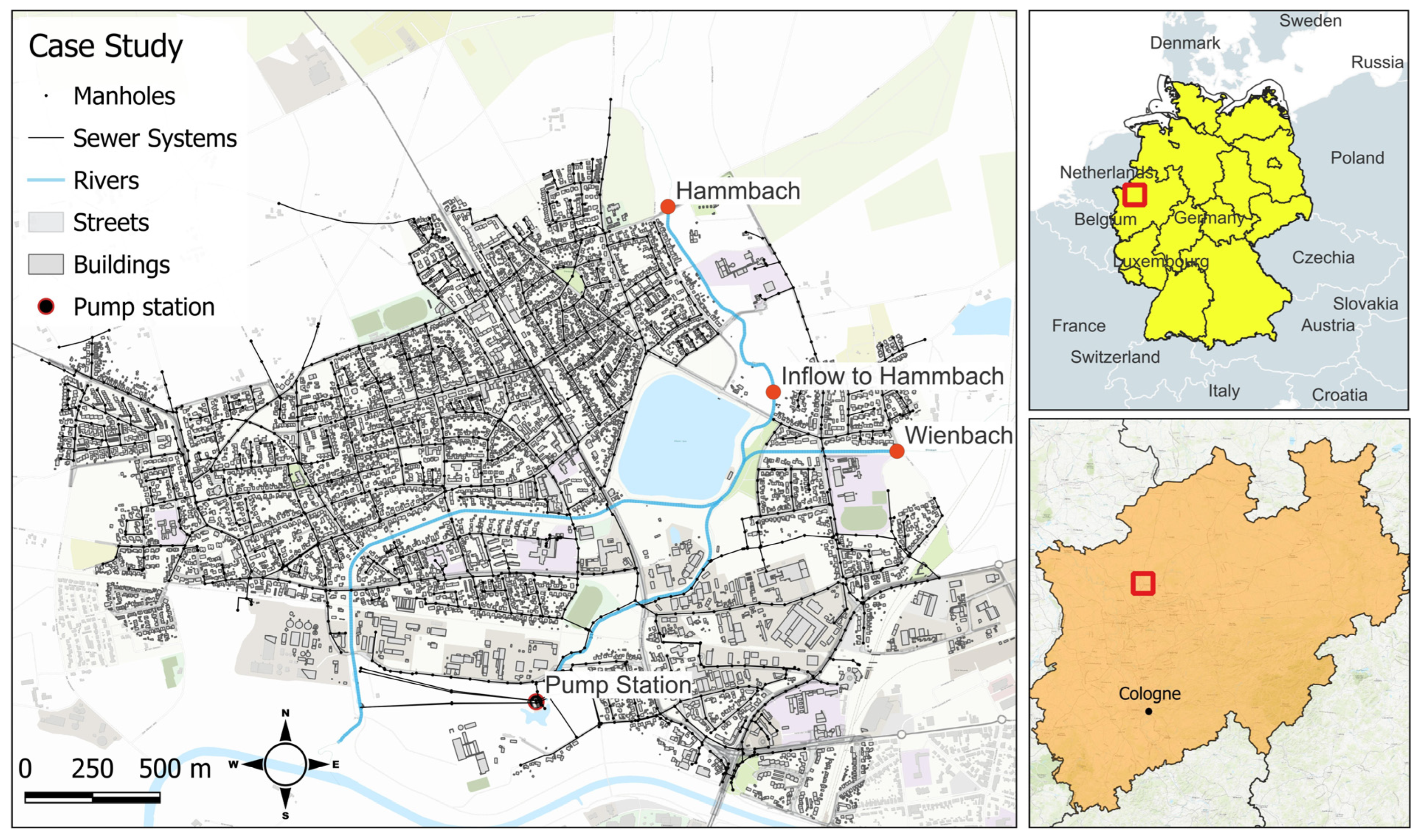
Figure 1. Study area in Dorsten with the pumping station in the south and three inflows. Basemap: Esri, Topographic Basemap; sources: Esri, Garmin, FAO, NOAA, USGS Administrative boundaries: © Federal Agency for Cartography and Geodesy (BKG), 2024, VG250, licensed under CC BY 4.0.
Water 17 02876 g001
Figure 2. Framework to derive a flood probability map considering different failure scenarios of a pumping station with several pumps.
Water 17 02876 g002
Figure 3. Example of a network with random variables A–E (nodes) and edges (arcs). A represents the root node, which is seen as independent. B-E represent child nodes, whereas C is also a parent node for B, D, and E.
Water 17 02876 g003
Figure 4. Bayesian network with precondition variables in blue as initial parameter (a priori knowledge), dependent variables in brown, and scenarios leading to pump failure in red. The dependency between the variables is represented by arcs.
Water 17 02876 g004
Figure 5. Flood extent maps of failure scenarios 1–7 (ag) and scenario 8 (h) with no failure for a rainfall event with a 100-year return period. Cells assigned to class 1 (blue) are seen as wet with a defined threshold of 0.1 m. Cells assigned to class 0 are seen as dry.
Water 17 02876 g005aWater 17 02876 g005b
Figure 6. Example of a flood inundation probability map for a rainfall event with 100-year return period, considering all failure scenarios. Light red areas have the lowest probability of flooding and dark red areas the highest.
Water 17 02876 g006
Table 1. Overview of stormwater pumps in the pumping station.
Pump IDPump Discharge Capacity [m3/s]
Pump 12
Pump 24.5
Pump 34.5
Pump 44.5
Table 2. All possible failure scenarios with corresponding total-pumping discharge capacity.
ScenarioPump Discharge Capacity [m3/s]
Pump ID 1
Pump Discharge Capacity [m3/s]
Pump ID 2
Pump Discharge Capacity [m3/s]
Pump ID 3
Pump Discharge Capacity [m3/s]
Pump ID 4
Total-Pumping Discharge Capacity [m3/s]
10.00.00.00.00.0
22.04.54.50.011.0
32.04.50.04.511.0
42.00.04.54.511.0
50.04.54.54.513.5
62.04.50.00.06.5
72.00.04.50.06.5
82.00.00.04.56.5
90.04.54.50.09.0
100.04.50.04.59.0
110.00.04.54.59.0
122.00.00.00.02.0
130.04.50.00.04.5
140.00.04.50.04.5
150.00.00.04.54.5
Table 3. Failure scenarios considering total-pumping discharge capacity.
ScenarioTotal-Pumping Discharge Capacity [m3/s]
10
211
313.5
46.5
59
62
74.5
Table 4. Example of probability assignment on the basis of electricity supply being available.
Type of Supply
Severe weatherSingleDual
Yes92%97%
No98%99%
Table 5. Example for the initial variables considering three different scenarios.
VariableRegular Operation
(Pump 1–4)
Flood Scenario
(Pump 1–4)
Extreme Scenario
(Pump 1–4)
Pump state (on/off)OnOnOff
Power supplyDual power supplyDual power supplyDual power supply
severe weatherNoYesYes
Waterproof constructionYesYesYes
Incoming dischargebelow design dischargeabove design dischargeabove design discharge
Age of Pumps (1–4)(3, 8, 20, 14)(3, 8, 20, 14)(3, 8, 20, 14)
Sediment protectionYesYesYes
Rinsing nozzlesYesYesYes
Flooding in the past few daysNoNoYes
Regular maintenanceYesYesNo
Table 6. Failure probabilities of each pump with set a priori knowledge are shown in Table 5.
Scenarios/Failure ProbabilityRegular Operation
[%]
Flood Scenario
[%]
Extreme Scenario
[%]
Pump 112362
Pump 222564
Pump 352978
Pump 432770
Table 7. Derived probabilities of pump states (on/off).
Pumps/State
(Flood Scenario)
Operating
Probability [%]
Failure
Probability [%]
Pump 17723
Pump 27525
Pump 37129
Pump 47327
Table 8. Derived occurrence probability for each pump and the corresponding scenario.
ScenarioPump 1
[%]
Pump 2
[%]
Pump 3
[%]
Pump 4
[%]
Scenario Probability
[%]
Total-Pumping Discharge Capacity
[m3/s]
123.025.029.027.00.50.0
277.075.071.027.011.111.0
377.075.029.073.012.211.0
477.025.071.073.010.011.0
523.075.071.073.08.913.5
677.075.029.027.04.56.5
777.025.071.027.03.76.5
877.025.029.073.04.16.5
923.075.071.027.03.39.0
1023.075.029.073.03.79.0
1123.025.071.073.03.09.0
1277.025.029.027.01.52.0
1323.075.029.027.01.44.5
1423.025.071.027.01.14.5
1523.025.029.073.01.24.5
Table 9. Occurrence probability of each failure scenario and of no failure (=scenario 8).
ScenarioTotal-Pumping Discharge Capacity [m3/s]Residual-Pumping Discharge Capacity [%]Occurrence
Probability [%]
100.00.5
21171.033.3
313.587.18.9
46.541.912.3
5958.19.9
6212.91.5
74.529.03.7
815.5100.029.9
Disclaimer/Publisher’s Note: The statements, opinions and data contained in all publications are solely those of the individual author(s) and contributor(s) and not of MDPI and/or the editor(s). MDPI and/or the editor(s) disclaim responsibility for any injury to people or property resulting from any ideas, methods, instructions or products referred to in the content.