Article

Research on Acceleration Methods for Hydrodynamic Models Integrating a Dynamic Grid System, Local Time Stepping, and GPU Parallel Computing

1
Power China Eco-Environmental Group Co., Ltd., Shenzhen 518101, China
2
Pearl River Water Resources Research Institute, Guangzhou 510611, China
*
Author to whom correspondence should be addressed.
Water 2025, 17(18), 2662; https://doi.org/10.3390/w17182662
Submission received: 30 June 2025 / Revised: 16 August 2025 / Accepted: 28 August 2025 / Published: 9 September 2025
(This article belongs to the Section Hydraulics and Hydrodynamics)

Abstract

Alongside the development of smart water management and digital twin construction, hydrodynamic models have become a critical scientific tool in flood forecasting, with increasing attention and research focused on model computational efficiency. At the algorithmic optimization level, employing a domain tracking method reduces the number of grid cells actively involved in computation, while utilizing local time stepping techniques increases the average time step for updating model variables; integrating these methods reduces the overall computational load during simulation and enhances computational efficiency. At the hardware level, acceleration technologies such as GPU parallel computing can be utilized to fully exploit hardware capabilities and improve computational efficiency. A novel hydrodynamic model acceleration method combining algorithmic optimization and parallel computing techniques has been proposed, with the integrated method simultaneously reducing computational workload and improving model performance. Case tests demonstrated that this integrated approach could achieve a considerable computational speed-up ratio compared to traditional serial programs without algorithmic optimization. The integrated method effectively enhanced computational efficiency and maintained the model’s computational accuracy, ultimately fulfilling the dual requirements of precision and speed in practical hydrodynamic modeling applications.

1. Introduction

Against the backdrop of global warming and accelerated urbanization, 40% (195,000 km2) of the global urban land will be projected to be located in high-frequency flood zones by 2030 [1]. Flood disasters have emerged as one of the most critical natural hazards [2], posing significant threats to public safety and constraining socioeconomic development [3]. Effective decision support tools are important in gathering information to facilitate transparent decision-making process in order to evaluate and plan urban resilience to flooding. Two-dimensional (2D) hydrodynamic models, which mathematically simulate surface flow processes to predict flood propagation under varying conditions, have become indispensable scientific tools for flood risk management [4]. With the recent advancements in water management systems and digital twin systems for water conservancy, operational requirements for hydrodynamic models—particularly in terms of spatial–temporal resolution and computational efficiency—have escalated substantially [5]. However, achieving higher grid resolution in 2D models incurs exponential computational costs: doubling the grid resolution usually leads to a fourfold increase in grid cells and a halving of the permissible time step under the Courant–Friedrichs–Lewy (CFL) stability condition, resulting in an eightfold surge in overall computational workload [4]. This dramatic complexity growth severely limits model usability for real-time applications [6,7].
Many publicly available hydrodynamic models (e.g., HEC-RAS) are widely used in scientific research and engineering applications [8]. However, these software tools primarily rely on solving governing equations to achieve accurate simulation of flood evolution processes at the CPU-based serial computing level. Detailed studies on algorithmic optimization methods for efficient model computation remain scarce in these model’s research. To address this challenge, various computational acceleration strategies have been proposed, among which algorithmic optimization represents a critical category. Spatially, flood processes typically exhibit localized characteristics, enabling the implementation of domain tracking method. This approach selectively activate computational grids only within inundation-prone regions while deactivating irrelevant cells [9]. By reducing steps in both flux calculations and state variable updates, it achieves approximately 50% reduction in computational costs [10]. Temporally, traditional models employ globally uniform time steps dictated by the strictest CFL condition across all grids. Local time-stepping (LTS) techniques overcome this limitation by assigning grid-specific time steps tailored to local CFL constraints, significantly reducing redundant calculations [11,12,13,14,15].
Parallel computing has further revolutionized hydrodynamic modeling efficiency by leveraging high-performance computing architectures [16]. Saleem et al. [17] demonstrated a 331.51× speedup over CPU-based implementations by hybridizing MPI and OpenACC parallelization frameworks, while Dong et al. [18] achieved rapid flash flood simulations using multi-GPU acceleration. Additionally, beyond its high computational efficiency, GPU parallel computing exhibits an energy efficiency ratio (energy/frame(step)) 1–3 times higher than traditional CPU technologies for compute-intensive tasks such as hydrodynamic modeling [19,20].
Despite these advancements, GPU-based acceleration alone may still fall short of operational timeliness requirements for large-scale or long-duration simulations. Zhang et al. [21] highlighted the limited acceleration efficiency of single-GPU configurations under resource constraints, prompting research into synergistic combinations of GPU parallelization with algorithmic optimizations. Recent studies, such as Zhao et al.’s LTS-GPU coupled sediment transport model (1.49–2.38× efficiency gain) [22] and Hou et al.’s dynamic grid–GPU hybrid approach (50% additional speedup), underscore the potential of multi-strategy fusion [10].
The integration of dynamic grid adaptation, local time-stepping, and GPU parallelization forms the core of the proposed acceleration framework within the HydroMPM flood simulation platform [23]. Through systematic evaluation of these optimization techniques, this study seeks to provide a methodological reference for developing high-performance hydrodynamic models that address the computational demands of modern flood management [24].

2. High Performance Hydrodynamic Model

2.1. Base Model

The improved two-dimensional shallow water equations are adopted as the governing equations [12,24]:
U t + E x + G y = S
In which,
U = h h u h v ,
E = hu h u 2 + g h 2 b 2 2 huv ,
G = h v h u v h v 2 + g h 2 b 2 2 ,
S = 0 g h + b S 0 x g h S fx g h + b S 0 y g h S fy
where U is the conservation vector, E and G represent the flux vectors in the x and y directions, respectively, and S denotes the source term. Here, h represents water depth; u and v are the vertically averaged flow velocities in the x and y directions; b is the bed elevation; S0x and S0y are the bottom slope source terms in the x and y directions, defined as S0x = −∂b/∂x and S0y = −∂b/∂y; and Sfx and Sfy are the friction source terms in the x and y directions, expressed as Sfx = n2u√(u2 + v2)/h4/3 and Sfy = n2v√(u2 + v2)/h4/3.
For the numerical solution, the computational domain is discretized using an unstructured triangular mesh. A cell-centered finite volume method is employed to discretize the governing equations. The bed elevation b is defined at mesh nodes, while variables such as water depth, water level, and flow velocities are defined at cell centers. Numerical flux computation is performed using the approximate Riemann solver (Harten-Lax-van Leer-Contact, HLLC), and the equations are solved with the Monotone Upstream-centered Schemes for Conservation Laws (MUSCL) featuring second-order spatial–temporal accuracy. The computational modules mainly include: cell wet/dry state classification, slope calculation, prediction step, spatial reconstruction, Riemann problem solution, boundary condition treatment, source term processing, and correction step. Detailed numerical implementation procedures can be referenced in the literature [23].

2.2. Performance Optimization

2.2.1. Dynamic Grid System

In practical flood inundation processes, floodwater propagates from breach points or boundaries into the computational domain, gradually spreading outward under the influence of local terrain roughness. During certain or the entire simulation period, the number of effective computational cells (composed of wet cells and dry–wet interface cells) remains significantly smaller than the total grid count. As illustrated in Figure 1, at the initial stage of overtopping, only one grid cell within the domain is wet. To ensure proper surface flow propagation, an effective cell group is formed by selecting the wet cell and its two neighboring dry–wet interface cells. Accurate flood routing results can be obtained by performing flux calculations and cell variable updates solely for this effective cell group (Figure 1a). As surface flow continues to evolve due to local terrain features and sustained discharge from drainage networks, the inundation area expands with increasing wet cells. A new effective cell group, comprising wet cells and adjacent dry–wet interface cells, is dynamically formed to sustain continuous flood routing calculations (Figure 1b). Throughout the simulation, the number of grid cells in the effective cell group remains substantially smaller than the total model grid count. Implementing this dynamic mesh control strategy can significantly reduce computational workload and improve calculation efficiency [15].
The core steps of this dynamic mesh control algorithm involve dynamically updating the grid edges and cells participating in iterative calculations at each time step. Firstly, the necessity for flux calculation across each grid edge is determined by the water depths in adjacent cells: boundary edges or edges with at least one adjacent cell having h > 0 are designated as active computational edges, while others are excluded from calculations. Secondly, cell status is determined based on edge computational status: any cell containing at least one active computational edge is classified as an active computational cell, while cells with no active edges are excluded from calculations [13,14].

2.2.2. Local Time Step Technology

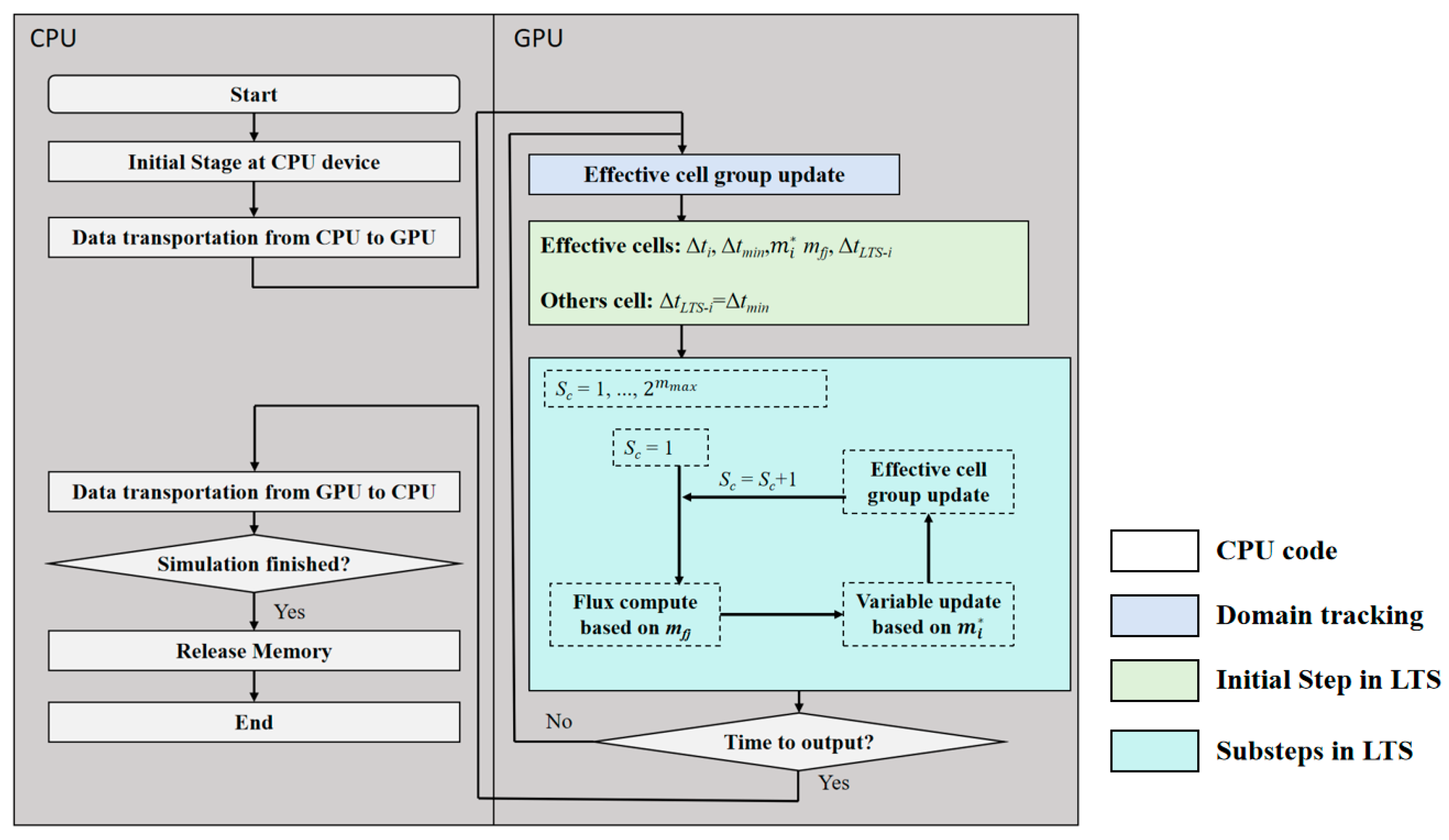
The local time-stepping technique reduces computational workload and enhances model efficiency through hierarchical computation and cell-wise updates. The specific implementation steps are as follows: ① Calculate the allowable maximum time step Δti for each grid cell based on the CFL condition (see Equation (2)); ② determine the global minimum time step Δtmin across all grid cells (see Equation (3)); ③ establish the local time-stepping levels (mi for cells and mfj for edges) for each grid cell and edge by comparing their individual maximum time steps with the global minimum (see Equations (4)–(6)); ④ finalize the local time step for each grid cell based on its assigned level (see Equation (7)); and ⑤ perform flux calculations and cell updates using the determined local time steps. The model advances globally when all local time-stepping cycles complete, with mmax = max(mi) representing the maximum acceleration level.
t i = Cr min l = 1 , 2 , , l   ( R il u il 2 + v i l 2 + g h i )
Δ t min = min i = 1 , 2 , Nc   { Δ t i }
m i = min [ int ( ln ( Δ t i / Δ t min ) l n 2 ) , m user ]
m fj = min j = 1 , 2 , , Nf   ( m jL , m jR )
m i * = min ( m i , m i1 m il )
Δ t LTS i = 2 m i * Δ t min
where uil and vil are the x- and y-components of the average flow velocity along the l-th edge of the i-th cell; hi denotes the water depth at the center of the i-th cell; Cr represents the Courant number; muser is a user-defined parameter limiting the time-stepping levels (muser = 0 corresponds to the conventional global minimum time-stepping algorithm, where ΔtLTS-i = Δtmin); mfj indicates the time-stepping level for the j-th edge; mjL and mjR are the time-stepping levels of the left and right cells adjacent to the j-th edge; mi-real denotes the actual implemented local time-stepping level; and ΔtLTS-i represents the final local time step for the i-th cell.
The variable update process using the local time-stepping (LTS) technique is illustrated with muser = 2. When mmax = muser = 2, The total number of sub-cycles required is Nsubstep = 4. As shown in Figure 2, grid cells/edges are assigned different time-stepping levels: cells with level 0 use Δtmin for updates, level 1 cells employ 2Δtmin, and level 2 cells utilize 4Δtmin.
In substep 1, only level 0 cells undergo updates (Figure 2a, the blue cells are indicated to be activated). In substep 2, both level 0 and level 1 cells are updated (Figure 2b). Substep 3 again updates only level 0 cells (Figure 2c). Finally, during substep 4, all cell levels (0, 1, and 2) are simultaneously updated (Figure 2d), completing a full synchronous update cycle across the entire domain.
Throughout this hierarchical update process, grid cells and edges participate in flux computations and variable updates in a staggered manner according to their assigned levels. Compared to the conventional global minimum time-stepping algorithm, this approach significantly reduces the number of active computational elements at each substep, thereby enhancing overall computational efficiency while maintaining numerical stability. The efficiency gain stems from: (1) avoiding redundant calculations on dry/static regions, and (2) allowing computationally intensive wet regions to advance with larger time steps within their assigned levels.

2.2.3. GPU Parallelization

In surface flood routing simulations, the most computationally intensive step involves iterative traversal of grid cells for numerical analysis. The core objective of GPU parallelization is to distribute these iterative computations across multiple threads, leveraging the massive thread parallelism of GPU hardware to significantly enhance model efficiency. Current GPU parallelization approaches primarily fall into two categories: implicit parallelism (directive-based, e.g., OpenACC) and explicit parallelism (kernel-based, e.g., CUDA). As a widely adopted explicit parallelism method, CUDA requires complete restructuring of original sequential loops into standardized kernel functions, with explicit specification of data transfer mechanisms and thread allocation schemes during kernel execution. For OpenACC code, detailed performance studies identifies that the lack of interface to access the on-chip memory can severely limit the performance when compared to hand-tuned CUDA code. The evaluations indicate that the current OpenACC compilers achieve approximately 50% of performance of the CUDA versions, reaching up to 98% depending on the compiler [25]. Therefore, this study adopts CUDA for model refactoring to attain superior computational speedup.

2.2.4. Fusion Method of Dynamic Mesh, Local Time-Stepping, and GPU Parallel Acceleration

Building on previous research, this study proposes an integrated methodology that synergistically combines dynamic mesh control strategy, local time-stepping (LTS) technique, and GPU parallel acceleration to enhance computational efficiency in flood inundation modeling. The approach begins with CPU-based model initialization and GPU memory allocation for data storage, followed by complete execution of computational workflows on the GPU. This involves: (1) identifying effective computational cells through dynamic mesh control to restrict calculations to relevant wet/dry–wet interface regions; (2) applying adaptive time-stepping levels based on local hydrodynamic conditions using LTS technology; (3) performing hierarchical model updates with staggered synchronization mechanisms; and (4) conditionally transferring results from GPU to CPU upon reaching output intervals for visualization and analysis. By fusing these three components—dynamic mesh refinement reducing active computational elements, LTS enabling time-adaptive updates without global synchronization overhead, and GPU parallelization exploiting hardware concurrency for loop-level acceleration—the proposed method achieves significant computational speedup while maintaining numerical fidelity. The complete algorithmic workflow of this integrated approach is illustrated in Figure 3, demonstrating the sequential execution of dynamic mesh adaptation, time-stepping level assignment, and parallel computation phases within the GPU environment.

3. Numerical Test

In this section, the numerical efficiency and accuracy of the proposed model to represent flash flood routine process is demonstrated by firstly considering a idealized flood cases over three humps. To further analyze the performance of the model, we considered a real flash flooding-prone area in China and three grid division schemes with different resolution. A NVIDIA RTX 4060 card is used in this work for GPU parallel computation. The time step is governed by the CFL number of 0.85 for all computation cases.

3.1. Dam Break Flow over Three Humps

This numerical case study focuses on dam-break wave propagation over a riverbed featuring three humps. The inundation process incorporates complex hydrodynamic phenomena including unsteady flow motion in intricate terrain, wet–dry boundary transitions, and frictional resistance effects. Therefore, this benchmark scenario has been widely adopted to verify model capabilities in numerical stability, complex topography representation, and dynamic boundary handling. The simulation domain consists of a rectangular basin measuring 75 m in length and 30 m in width, enclosed by solid walls and containing three conical obstacles. The bathymetric configuration is defined as follows:
z b ( x , y ) = max 0 ,   1 1 8 ( x 30 ) 2 + ( y + 9 ) 2 ,   1 1 8 ( x 30 ) 2 + ( y 9 ) 2 ,   3 3 10 ( x 47.5 ) 2 + y 2
where x, y indicates the location and z b ( x , y ) is the bed elevation.
Under initial conditions, a dam is positioned at x = 16 m, with 1.875 m deep quiescent water occupying the left side and a dry bed occupying the right side. The Manning’s roughness coefficient is set to 0.025. To investigate the impact of mesh resolution on computational and algorithmic efficiency, three distinct computational grids are employed: (1) Uniform triangular mesh (Figure 4a) with element edge length of 0.2 m, comprising 129,486 elements and 65,269 nodes; (2) non-uniform triangular mesh with localized refinement along the midline (Figure 4b) featuring minimum/maximum edge lengths of 0.1 m/0.2 m, containing 173,080 elements and 87,066 nodes; and (3) non-uniform triangular mesh with enhanced midline refinement (Figure 4c) having minimum/maximum edge lengths of 0.05 m/0.2 m, maintaining the same element and node counts as the second configuration (173,080 elements and 87,066 nodes).
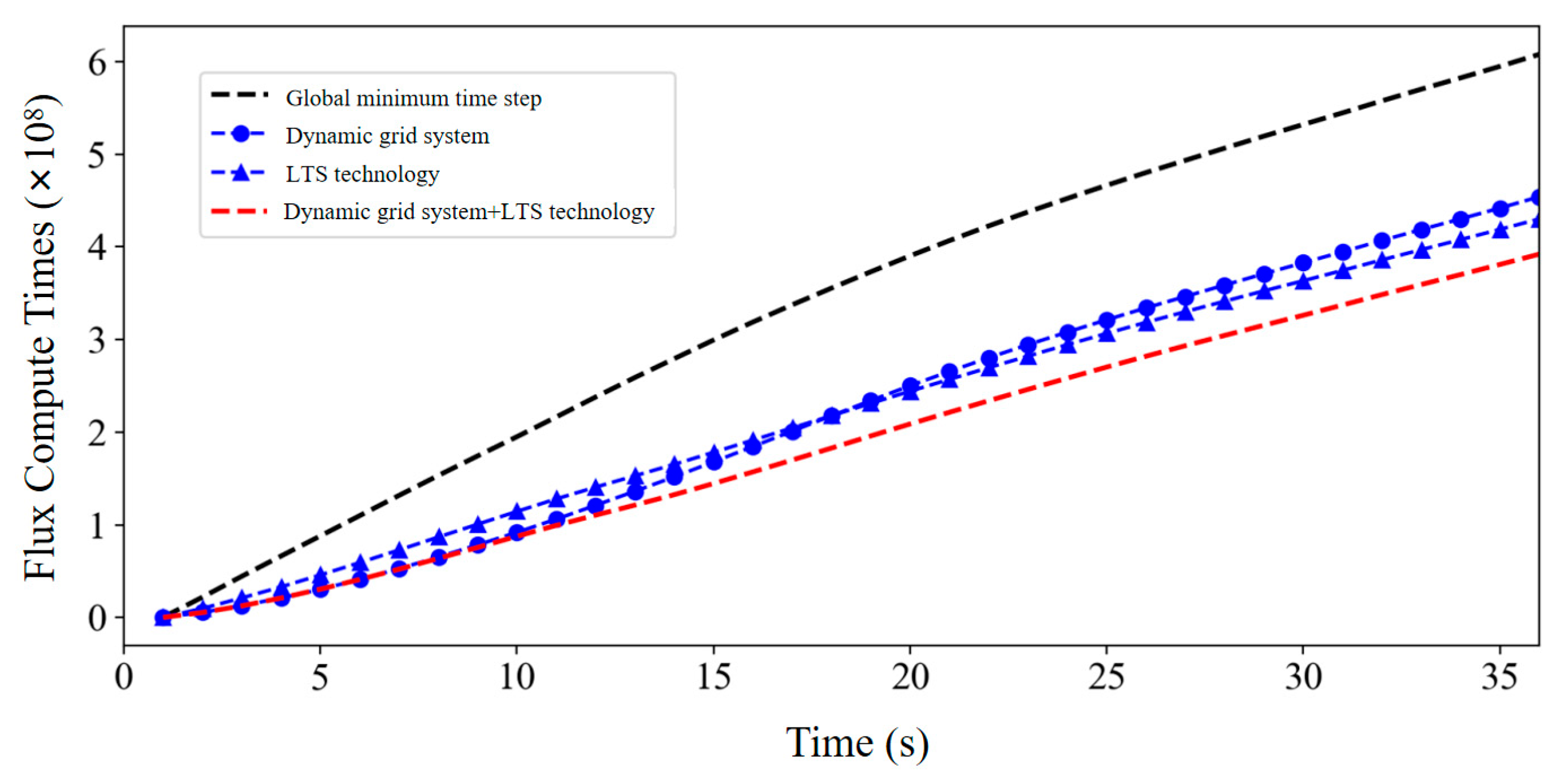
The local time-stepping (LTS) technique and dynamic mesh control strategy both enhance computational efficiency by reducing model workload. Figure 5 illustrates the cumulative flux computation counts (Riemann solver invocations for edge flux calculations) under different algorithmic configurations for the uniform triangular mesh (Grid a), analyzing the total computational burden throughout the simulation.
In the figure, the black curve represents the cumulative flux computations under the conventional global minimum time-stepping strategy. During the initial 18 s, the dam-break wave propagates over the dry bed on the tank’s right side, encountering complex flow patterns due to the three hump-shaped obstacles. This results in small time steps and rapid accumulation of flux computations. After 18 s, as the floodwater covers the entire basin and flow regimes stabilize, the cumulative flux count continues to grow linearly but with reduced slope, reaching 6.1 × 10⁸ at 36 s.
The two blue curves depict the flux computation trends under dynamic mesh control and LTS technique (muser = 2). Several observations emerge: (1) Both optimization strategies effectively reduce computational workload, but with different temporal effectiveness profiles. The dynamic mesh strategy demonstrates significant advantage during the first 18 s (dry-bed propagation phase) by restricting computations to submerged areas, resulting in lower cumulative counts than LTS. However, (2) after 18 s (full basin inundation), dynamic mesh optimization becomes ineffective while LTS maintains consistent reduction. Consequently, the dynamic mesh curve surpasses the LTS curve post-18 s, reaching 4.6 × 10⁸ versus 4.3 × 10⁸ at 36 s.
The red curve shows the hybrid strategy combining dynamic mesh and LTS techniques. By applying LTS exclusively to active computational regions, this fusion approach further reduces cumulative flux computations compared to standalone LTS. The hybrid method consistently maintains the lowest computation counts throughout the simulation, reaching 3.9 × 10⁸ at 36 s—approximately 20% reduction compared to the global minimum time-stepping baseline. It should be noted that while GPU parallelization accelerates computations, its effect on workload reduction is not reflected in this figure as it does not alter the total computation volume.
Table 1 summarizes the comparisons of cumulative flux computation counts and computational time for the three-hump dam-break benchmark under different mesh configurations and acceleration strategies. The results indicate that the dynamic mesh control strategy, local time-stepping technique, and GPU parallel acceleration technology all effectively enhance computational efficiency. Among these, GPU parallelization demonstrates the most significant acceleration effect, achieving a maximum speedup ratio of 49.06 in the test cases. Furthermore, the integrated application of dynamic mesh control, local time-stepping, and GPU parallel acceleration achieves a further improvement in computational efficiency beyond GPU acceleration alone, reaching a maximum speedup ratio of 62.98.

3.2. Simulation of Inundation Caused by Tuanzhouyuan Dyke Breach

Tuanzhouyuan is situated on the western shore of Dongting Lake, bordering Moshan Mountain to the north, Ouchi River to the south, Nanshan Mountain and Huarong Chenghu Embankment to the west. It encompasses Xinsheng Embankment, Qianlianghu South Embankment, Qianlianghu North Embankment, Xinhua Embankment, Tuanzhouyuan Embankment, Xintai Embankment, and Xiaotuanzhouyuan Embankment. The total length of the surrounding embankments is 146 km, protecting an area of 454 km2 with 330,000 mu (approximately 220 km2) of cultivated land and a population of 230,000 within the embankment zone. At approximately 16:00 on 5 July 2024, a piping incident occurred at the Tuanzhouyuan Embankment section along Dongting Lake, leading to subsequent dyke breach. Following the breach, the inundated area within Tuanzhouyuan Embankment expanded rapidly, resulting in widespread flooding by 6 July.
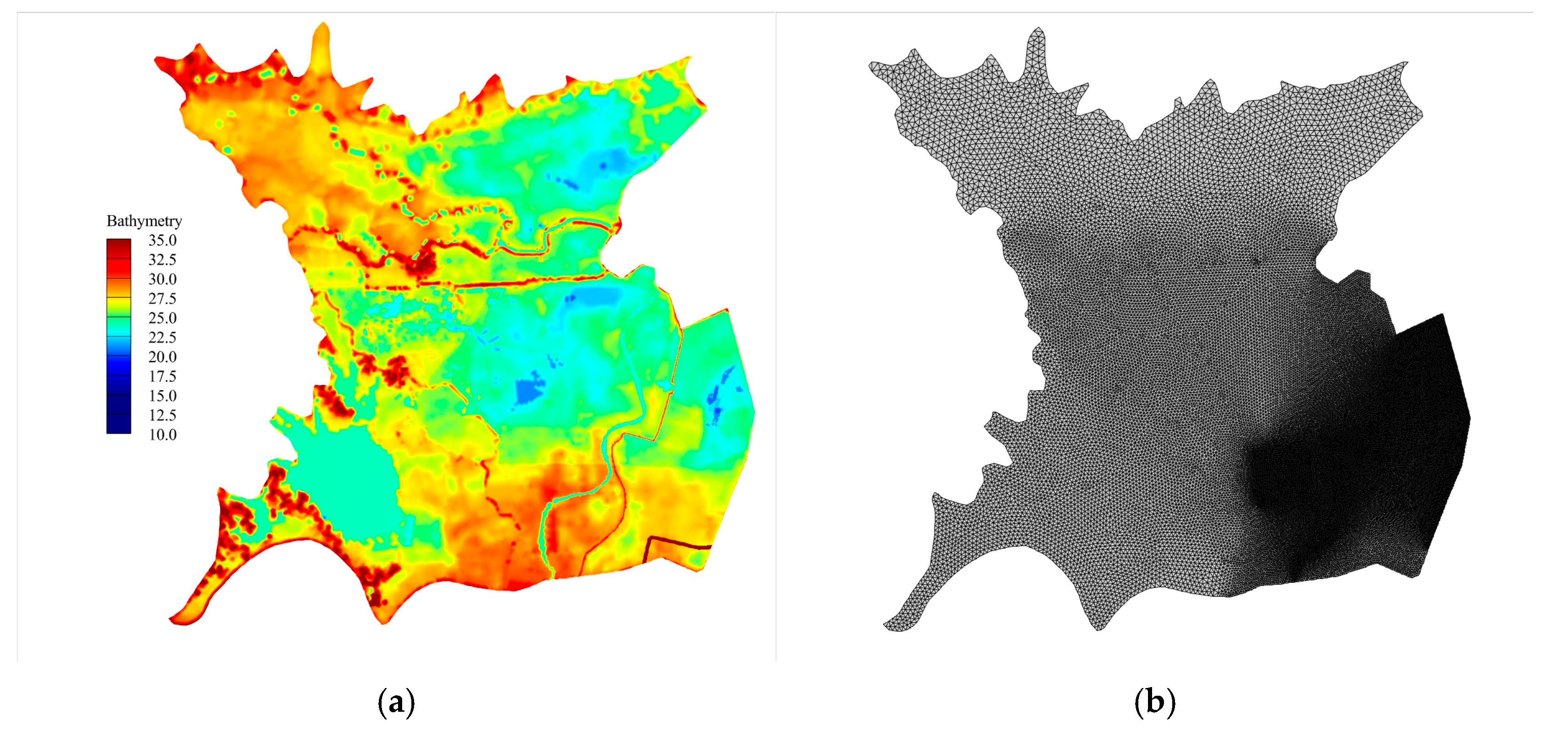
The individual embankments within Qianlianghu are separated by secondary levees, creating potential for cascading breach-induced flooding. Consequently, the modeling analysis encompassed the entire Tuanzhouyuan, with localized mesh refinement implemented for flooded area. The computational domain comprises 87,342 unstructured triangular elements, with minimum and maximum element edge lengths of 33 m and 300 m, respectively, as illustrated in Figure 6. Grid terrain elevations were interpolated from 10m-resolution DEM data, and the Manning roughness coefficient was uniformly set to 0.035 across the entire computational domain.
Following the dyke breach incident at Tuanzhouyuan Embankment, the Changjiang Water Resources Commission (CWRC) established two temporary hydrological monitoring stations—one inside and one outside the breach area—to continuously monitor water levels and estimate the discharge hydrograph at the breach site. The present analysis directly utilizes the discharge data from the temporary external monitoring station as boundary conditions to simulate the flood routing process from 18:00 on 5 July to 18:00 on 7 July. The simulated dynamic inundation evolution during this period is visualized in Figure 7. As shown in the figure, blocked by the Qiantuan intermediate dike within the computational domain, the breach flood primarily propagated along the eastern side of the calculation area. After 12 h, the flood had inundated most of the eastern region. However, since the floodwater level remained below the elevation of the intermediate dike, the western area remained unaffected by the inundation.
Following the breach occurrence, the Ministry of Water Resources continuously monitored the flood inundation extent within Tuanzhouyuan using satellite remote sensing data. For model calibration, we imported the unstructured triangular mesh (configured in Figure 6) into the latest HEC-RAS model. The computational results were compared with both the proposed model and satellite remote sensing-derived inundation areas, as shown in Figure 8. It is evident that for the Tuanzhouyuan dyke breach case, the computational outcomes of the proposed model align closely with those of the HEC-RAS model. Notably, while the mathematically modeled inundation extent appears slightly smaller than the satellite remote sensing inversion results (due to the latter treating elevated buildings above water surfaces as unflooded land), the overall trends demonstrate remarkable consistency, confirming the high accuracy of the proposed model.
During the Tuanzhouyuan breach simulation, the CPU serial version model required 46 min for computation, while the local time-stepping technique (muser = 2) reduced the computation time to 34 min, achieving a speedup ratio of 1.35. The dynamic meshing strategy further reduced the computation time to 28 min, corresponding to a speedup ratio of 1.64. When combining local time-stepping with dynamic meshing, the computation time was reduced to 24 min, resulting in a speedup ratio of 1.92. GPU parallel computing significantly reduced the computation time to 1.1 min, yielding a remarkable speedup ratio of 41.8. The computational efficiency reached approximately 26.5%. The integration of local time-stepping, dynamic meshing, and GPU parallel computing achieved a computation time of approximately 40 s, with a speedup ratio of 69 times, effectively meeting the requirements for real-time simulation of flood inundation processes. This demonstrates that the combined application of local time-stepping, dynamic meshing, and GPU parallel computing successfully integrates the advantages of these algorithms, showing excellent adaptability in simulating typical flood evolution scenarios involving dyke breaches and overflows.

4. Conclusions

Two-dimensional hydrodynamic models serve as critical components in flood simulation. However, as the computational mesh resolution increases, the number of grid cells and the associated computational load escalate significantly, leading to prolonged simulation times that hinder the broader application of hydrodynamic models. Notably, flood inundation processes typically initiate in localized areas before gradually expanding.
The dynamic mesh updating strategy enables efficient participation of active grid cells in computations, thereby reducing overall computational demands. Concurrently, given the complex flow regimes in flood scenarios, the local time-stepping technique allows individual grid cells to adaptively update variables using optimized time increments, further minimizing computational workload. Building upon the self-developed HydroMPM flood simulation framework, this study integrates GPU parallel computing technology with dynamic mesh control strategies and local time-stepping techniques.
Two typical numerical cases were used to test the efficacy of the hybrid approach. For the three-hump case, where nearly the entire computational domain was ultimately inundated, the dynamic mesh algorithm demonstrated less pronounced effectiveness, while local time-stepping and GPU parallel techniques achieved acceleration effects comparable to those reported in the previous literature. For the Tuanzhouyuan dyke breach case, where inundation only affected a portion of the computational domain, dynamic mesh adaptation, local time-stepping, and GPU parallelism all yielded significant performance improvements. Comparative analysis revealed that while hardware-level parallel acceleration (GPU implementation) substantially enhanced computational efficiency (with pure GPU speedup ratios reaching 49× and 41.8×), the hybrid algorithm further reduced total computational workload on top of GPU acceleration, thereby achieving superior efficiency gains.
Regarding the metric of total model runtime, which is influenced by factors such as grid resolution, cell count, and simulation duration, neither GPU parallelism nor the hybrid algorithm can fully guarantee real-time performance (e.g., simulation time under 1 min). However, the proposed hybrid approach remains effective, and integrating multi-GPU parallelism to distribute computational loads across nodes could potentially meet stringent timing requirements. This constitutes a key direction for future research.

Author Contributions

Data curation, Y.P.; Formal analysis, H.X.; Methodology, L.S.; Investigation, J.C. and Z.Z.; Software and Writing, Y.H. All authors have read and agreed to the published version of the manuscript.

Funding

This research was funded by Research Center Targeted Funding Program of Power Construction Corporation of China, DJ-PTZX-2024-06.

Data Availability Statement

The raw data supporting the conclusions of this article will be made available by the authors on request.

Conflicts of Interest

Author Yang Ping was employed by the company Power China Eco-Environmental Group Co., Ltd. The remaining authors declare that the research was conducted in the absence of any commercial or financial relationships that could be construed as a potential conflict of interest. The authors declare that this study received funding from Research Center Targeted Funding Program of Power Construction Corporation of China, DJ-PTZX-2024-06. The funder was not involved in the study design, collection, analysis, interpretation of data, the writing of this article, or the decision to submit it for publication.

References

  1. Güneralp, B.; Güneralp, I.; Liu, Y. Changing global patterns of urban exposure to flood and drought hazards. Glob. Environ. Change 2015, 31, 217–225. [Google Scholar] [CrossRef]
  2. Rentschler, J.; Salhab, M.; Jafino, B.A. Flood exposure and poverty in 188 countries. Nat. Commun. 2022, 13, 3527. [Google Scholar] [CrossRef]
  3. Cea, L.; Sañudo, E.; Montalvo, C.; Farfán, J.; Puertas, J.; Tamagnone, P. Recent advances and future challenges in urban pluvial flood modelling. Urban Water J. 2025, 22, 149–173. [Google Scholar] [CrossRef]
  4. Kim, B.; Sanders, B.F.; Famiglietti, J.S.; Guinot, V. Urban flood modeling with porous shallow-water equations: A case study of model errors in the presence of anisotropic porosity. J. Hydrol. 2015, 523, 680–692. [Google Scholar] [CrossRef]
  5. Pal, D.; Marttila, H.; Ala-Aho, P.; Lotsari, E.; Ronkanen, A.-K.; Gonzales-Inca, C.; Croghan, D.; Korppoo, M.; Kämäri, M.; van Rooijen, E.; et al. Blueprint conceptualization for a river basin’s digital twin. Hydrol. Res. 2025, 56, 197–212. [Google Scholar] [CrossRef]
  6. Fernández-Pato, J.; García-Navarro, P. An Efficient GPU Implementation of a Coupled Overland-Sewer Hydraulic Model with Pollutant Transport. Hydrology 2021, 8, 146. [Google Scholar] [CrossRef]
  7. Mignot, E.; Dewals, B. Hydraulic modelling of inland urban flooding: Recent advances. J. Hydrol. 2022, 609, 127763. [Google Scholar] [CrossRef]
  8. USACE 2024b. HEC-RAS Version 6.6 Release Notes. Available online: https://www.hec.usace.army.mil/confluence/rasdocs/rasrn/latest (accessed on 8 October 2024).
  9. Judi, D.R.; Burian, S.J.; McPherson, T.N. Two-Dimensional Fast-Response Flood Modeling: Desktop Parallel Computing and Domain Tracking. J. Comput. Civ. Eng. 2011, 25, 184–191. [Google Scholar] [CrossRef]
  10. Hou, J.-M.; Wang, R.; Jing, H.-X.; Zhang, X.; Liang, Q.-H.; Di, Y.-Y. An efficient dynamic uniform Cartesian grid system for inundation modeling. Water Sci. Eng. 2017, 10, 267–274. [Google Scholar] [CrossRef]
  11. Sanders, B.F. Integration of a shallow water model with a local time step. J. Hydraul. Res. 2008, 46, 466–475. [Google Scholar] [CrossRef]
  12. Hu, P.; Lei, Y.; Han, J.; Cao, Z.; Liu, H.; He, Z.; Yue, Z. Improved Local Time Step for 2D Shallow-Water Modeling Based on Unstructured Grids. J. Hydraul. Eng. 2019, 145, 06019017. [Google Scholar] [CrossRef]
  13. Tao, J.; Hu, P.; Xie, J.; Ji, A.; Li, W. Application of the tidally averaged equilibrium cohesive sediment concentration for determination of physical parameters in the erosion-deposition fluxes. Estuar. Coast. Shelf Sci. 2024, 300, 108721. [Google Scholar] [CrossRef]
  14. Li, W.; Liu, B.; Hu, P. Fast modeling of vegetated flow and sediment transport over mobile beds using shallow water equations with anisotropic porosity. Water Resour. Res. 2023, 59, e2021WR031896. [Google Scholar] [CrossRef]
  15. Li, W.; Zhang, Y.; Hu, P. Fully coupled morphological modelling under the combined action of waves and currents. Adv. Water Resour. 2025, 195, 104875. [Google Scholar] [CrossRef]
  16. Sanders, J.; Kandrot, E. CUDA by Example: An Introduction to General-Purpose GPU Programming; Addison-Wesley: Boston, MA, USA, 2010. [Google Scholar]
  17. Saleem, A.H.; Norman, M.R. Accelerated numerical modeling of shallow water flows with MPI, OpenACC, and GPUs. Environ. Model. Softw. 2024, 180, 11. [Google Scholar] [CrossRef]
  18. Dong, B.; Huang, B.; Tan, C.; Xia, J.; Lin, K.; Gao, S.; Hu, Y. Multi-GPU parallelization of shallow water modelling on unstructured meshes. J. Hydrol. 2025, 657, 133105. [Google Scholar] [CrossRef]
  19. Qasaimeh, M.; Denolf, K.; Lo, J.; Vissers, K.; Zambreno, J.; Jones, P.H. Comparing Energy Efficiency of CPU, GPU and FPGA Implementations for Vision Kernels. In Proceedings of the 2019 IEEE International Conference on Embedded Software and Systems (ICESS), Las Vegas, NV, USA, 2–3 June 2019. [Google Scholar] [CrossRef]
  20. Lastovetsky, A.; Manumachu, R.R. Energy-Efficient Parallel Computing: Challenges to Scaling. Information 2023, 14, 248. [Google Scholar] [CrossRef]
  21. Zhang, Y.-Y.; Xu, W.-J.; Tian, F.-Q.; Du, X.-H. A Multi-GPUs based SWE algorithm and its application in the simulation of flood routing. Adv. Water Resour. 2025, 201, 104985. [Google Scholar] [CrossRef]
  22. Zhao, Z.; Hu, P.; Li, W.; Cao, Z.; Li, Y. An engineering-oriented Shallow-water Hydro-Sediment-Morphodynamic model using the GPU-acceleration and the hybrid LTS/GMaTS method. Adv. Eng. Softw. 2024, 200, 103821. [Google Scholar] [CrossRef]
  23. Hu, X.; Song, L. Hydrodynamic modeling of flash flood in mountain watersheds based on high-performance GPU computing. Nat. Hazards 2017, 91, 567–586. [Google Scholar] [CrossRef]
  24. Guo, K.; Guan, M.; Yu, D. Urban surface water flood modelling—A comprehensive review of current models and future challenges. Hydrol. Earth Syst. Sci. 2021, 25, 2843–2860. [Google Scholar] [CrossRef]
  25. Hoshino, T.; Maruyama, N.; Matsuoka, S.; Takaki, R. CUDA vs. OpenACC: Performance Case Studies with Kernel Benchmarks and a Memory-Bound CFD Application. In Proceedings of the 2013 13th IEEE/ACM International Symposium on Cluster, Cloud, and Grid Computing, Delft, The Netherlands, 13–16 May 2013; pp. 136–143. [Google Scholar] [CrossRef]
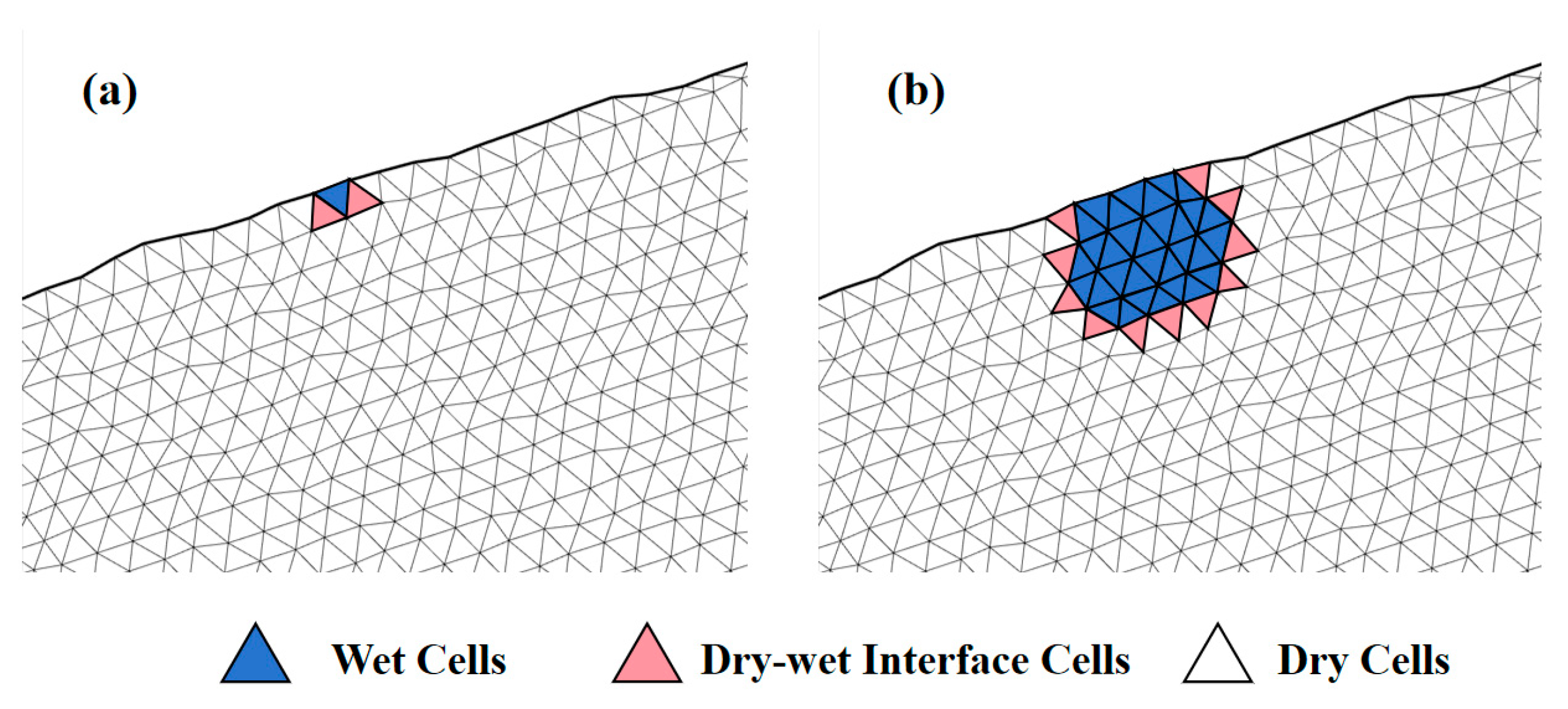
Figure 1. Schematic of dynamic mesh update strategy. (a) Initial effective cell group; (b) updated effective cell group.
Water 17 02662 g001
Figure 2. Schematic of grid update strategy for local time-stepping technique.
Water 17 02662 g002
Figure 3. Schematic of the integrated computational principle combining dynamic mesh, local time-stepping, and GPU parallel technologies.
Water 17 02662 g003
Figure 4. Mesh configuration for the three-hump dam-break benchmark. (a) Uniform triangular mesh; (b) non-uniform triangular mesh with midline refinement (minimum element size: 0.1 m); (c) non-uniform triangular mesh with midline refinement (minimum element size: 0.05 m).
Water 17 02662 g004
Figure 5. Comparison of cumulative flux computation counts under different algorithmic conditions.
Water 17 02662 g005
Figure 6. Modeling area of Inundation Caused by Tuanzhouyuan Dyke Breach. (a) Bethmetry of modeling area; (b) computation mesh of modeling area.
Water 17 02662 g006
Figure 7. Schematic Diagram of Simulated Flood Evolution Process in Tuanzhouyuan. (a) Simulated Flood Routing area at 1 h; (b) simulated Flood Routing area at 3 h; (c) simulated Flood Routing area at 6 h; (d) simulated Flood Routing area at 12 h.
Water 17 02662 g007
Figure 8. Comparison of Model-Calculated Inundation Area and Remotely Sensed Inversion-Derived Inundation Area.
Water 17 02662 g008
Table 1. Comparison of computational time and speed up ratio for the three-hump dam-break benchmark case under different mesh configurations and acceleration strategies.
CaseMesh InfoComputational Costs for Base Model/minSpeed Up Ratio
NumberMinimum SizeDynamic GridLTS TechnologyGPUDynamic Grid + LTSDynamic Grid + LTS + GPU
Uniform1294860.22.631.181.2915.81.4116.21
Non-uniform 2437900.111.341.091.3638.451.3341.58
Non-uniform 4742760.0539.921.181.5649.061.7862.98
Disclaimer/Publisher’s Note: The statements, opinions and data contained in all publications are solely those of the individual author(s) and contributor(s) and not of MDPI and/or the editor(s). MDPI and/or the editor(s) disclaim responsibility for any injury to people or property resulting from any ideas, methods, instructions or products referred to in the content.