Abstract
This study investigates the capability of Gaussian process regression (GPR) models in the probabilistic forecasting of water flow and depth in a combined sewer system. Traditionally, deterministic methods have been implemented in sewer flow forecasting and anomaly detection, two crucial techniques for a good wastewater network and treatment plant management. However, with the uncertain nature of the factors impacting on sewer flow and depth, a probabilistic approach which takes uncertainties into account is preferred. This research introduces a novel use of GPR in sewer systems for real-time control and forecasting. To this end, a composite kernel is designed to capture flow and depth patterns in dry- and wet-weather periods by considering the underlying physical characteristics of the system. The multi-input, single-output GPR model is evaluated using root mean square error (RMSE), coverage, and differential entropy. The model demonstrates high predictive accuracy for both treatment plant inflow and manhole water levels across various training durations, with coverage values ranging from 87.5% to 99.4%. Finally, the model is used for anomaly detection by identifying deviations from expected ranges, enabling the estimation of surcharge and overflow probabilities under various conditions.
1. Introduction
Sewer systems convey domestic, industrial and commercial wastewater (and sometimes stormwater and groundwater) from their sources to a wastewater treatment plant (WWTP) or a discharge point. These systems can be mainly divided into combined and separate sewer systems [1]. Combined sewer systems are built to take both wastewater and stormwater from different sources and convey them to the final point of the system. Such systems are prevalent in the UK, with Victorian era infrastructure deployed in the form of combined drainage systems in many urban areas.
Wastewater flow contains various types of pollutants which should be effectively treated to provide a safe environment. However, for several reasons, there are untreated releases in almost every sewer system which are detrimental to the environment and health [2]. The most important case in untreated wastewater releases is the combined sewer overflow (CSO), which is a structure installed to spill wastewater into the environment to reduce the risk of backup discharges and manhole overflows [3]. Even though CSOs minimise the risk of manhole overflows, blockages or pump failures, caused by various factors such as sediment formation [4], may still lead to unintentional discharges [5].
Given the adverse effects that CSOs cause, sewer systems should be designed and maintained in such a way that overflows are reduced to a minimum. Moreover, water companies risk paying penalties due to regulatory requirements set by the Water Service Regulation Authority (OFWAT) in the UK (and similar authorities in other countries). Therefore, water companies seek methods and models to predict the flow and to be able to forecast overflows in the system because proactive responses are often more cost-effective and preferable for mitigating environmental risks. However, reactive control is the most frequently implemented approach [6].
There are three types of models that can be used in forecasting overflows and other characteristics of a hydraulic or hydrologic environment: simulators [7], data-driven surrogate models [8] and hybrid models [9]. The first models, also known as physical models, have been used for more than five decades; however, they have been considered computationally expensive for years [10]. These models simulate the underlying physics of the environment and represent it as a set of partial differential equations (PDEs) [11].
The mathematical modelling of every physical system often requires tremendous simplifications that lead to significant uncertainties in computation. Additionally, high computational cost [12], demand for updating model parameters in response to urban development [13], and lack of knowledge of every physical behaviour of the system [13] are known as drawbacks of these models. Confidence in input parameters like the network topology, invert levels and current levels of service (for example root ingress, sediment build up, etc.) creates uncertainty in such models which can typically be improved through calibration approaches using short-term flow surveys at key nodes in the network to some extent.
On the other hand, data-driven models are capable of making predictions with greater computational efficiency [14]. These models present an opportunity to capture relationships between parameters without considering interactions [15]. Nonetheless, data-driven modelling suffers from a lack of physical interpretation, which may make it unreliable or challenging to interpret [16]. Therefore, some researchers have come to a mixture of data-driven and physical models, called physics-informed surrogate models, taking advantage of both physical and data-driven models [17]. While these models benefit from physical constraints, development and integrity challenges along with added complexity make them challenging to implement in this study and similar works.
Data-driven models range from simple linear regressions to complex deep-learning architectures, each varying in computational complexity. These models can be classified into deterministic and probabilistic approaches based on the way they handle uncertainty in the modelling process. While deterministic models offer an explicit solution to a water-related issue, probabilistic models take the inherent uncertainties of the data and the model parameters into account.
In sewer system modelling, uncertainties arise from multiple sources, including variability in precipitation and water usage, simplifications in physical equations, and sensor inaccuracies [18]—all of which can significantly impact the reliability of predictions. While most research in uncertainty quantification has focused on water quality and treatment plant operations, some researchers have addressed flow-related uncertainty. For example, Breinholt [19] assessed the uncertainty in flow prediction and modelling in a sewer system with a frequentist stochastic approach. Raimondi et al. [20] adopted a deterministic framework to quantify uncertainty in flow rate and temperature, while Sriwastava et al. [21] employed stochastic sampling to evaluate CSO volume variability.
While many data-driven models, like artificial neural networks (ANNs) and support vector machines (SVMs), require large datasets and lack uncertainty quantification in predictions, the Gaussian processes (GPs) method provides an approach capable of handling complex and small datasets through a natural Bayesian interpretation [22]. This method makes predictions incorporating experts’ prior knowledge with a model (called likelihood, i.e., a function showing the probability of data happening given a parameter) and provides uncertainty measures in its predictions [23]. Moreover, GP is known as a suitable method for working with rare and costly data, while it can provide good results with larger datasets with an O(N3) computational complexity (Computational complexity describes how the runtime of an algorithm scales with the size of the input data (N). An O(N3) complexity means the computation time increases with the cube of the number of training points) [16].
Gaussian process regression (GPR) has been implemented in many different fields of study due to its capability in uncertainty quantification and flexibility (i.e., the ability to emulate different function shapes). This capability has led GPR models to be used in engineering and scientific fields as surrogate models, such as in computational engineering [24], climate science [11], finance [25] and many time-series related forecasting models [26].
In water engineering, GP-based frameworks have been used in forecasting river streamflow [27] and reservoir streamflow [28], fault detection in wastewater treatment plants [29], evaluation of the flooded nodes in a sewer system [30], drinking water demand prediction [31], streamflow temperature forecasting [32], water level fluctuations forecasting [33] and approximating parameters of a storm water management model (SWMM) [12].
Due to the need for a model that combines computational efficiency with principled uncertainty quantification, this work presents a framework that deploys a GPR model for forecasting flow and depth in a sewer system. This model uses a custom-designed kernel to capture various patterns affecting flow and depth changes in different parts of the network. This probabilistic model aids water companies in making short- and mid-term asset management plans and responding proactively to potential issues in the network and treatment facilities.
In addition to what data-driven and particularly GPR models can forecast in wastewater systems, they offer valuable applications in real-time control and nowcasting. With abundant sensors placed in sewer systems, smart and monitored wastewater management is on the horizon [34]. One critical challenge in sewer systems is anomaly detection [35]. When a pump failure occurs or a blockage develops in a pipe, the water flow and depth suddenly decrease downstream while increasing upstream. The timely prediction of these anomalies plays an important role in urban water management [36] and reduces costs associated with pollution events driven by such issues [37].
Data-driven methods provide a more cost-effective alternative to hardware-based techniques (e.g., CCTV, acoustic sensing, etc.) [36,38]. Among them, probabilistic methods are credited for their ability to take complexities into account [39]. Nonetheless, there is no systematic research using GPR for detecting anomalies in a sewer system.
Accordingly, this research proposes a novel probabilistic method for anomaly detection using a GPR model. The method estimates the likelihood of blockage occurrences in real time, and raises alarms when discrepancies exceed predefined thresholds. This method can replace traditional deterministic approaches used by water companies, ensuring a safe environment with less uncontrolled overflows.
The remainder of this paper is organised as follows. Section 2 discusses the data and the hydraulic model used to prepare the training and test datasets. It also outlines the GPR model structure, its implementation within the framework, and the evaluation metrics applied to assess its performance.
Section 3 presents the results taken from the GPR model along with a discussion. It shows how the GPR model works with long- and short-term training periods and how it can be used in presenting probabilistic results for the stakeholders. Finally, the paper concludes with remarks and suggestions for future work.
2. Materials and Methods
2.1. Data and the Case Study
The case study of this research is a hypothetical combined sewer system built by EPA SWMM v5.2 software [40]. The system is a skeleton sewer network serving 11,300 inhabitants of a city, assumed to be placed in the UK. The average water consumption is assumed to be 140 Litre per capita per day with a 100% wastewater generation rate. A snapshot of the system and the details are presented in Figure 1 and Table 1.

Figure 1.
Skeleton sewer system terminating at the WWTP on the right side of the figure. The hatched areas show the sub-catchments, the links show the main sewers, and the square points are the Nodes labelled in the figure. The rain gauge (RG1) is shown at the right bottom of the figure.

Table 1.
Details of the wastewater production values and infiltration in each sub-catchment.
A CSO is set in the network to release excess flows via a weir. There is also a storage tank and a pumping station set to regulate the flow in the network. The mains and trunk sewers have been designed based on the IDF curves of London [41] and have sizes between 500 mm and 1200 mm.
Groundwater infiltration can have a major contribution to the flow of a sewer system which makes it important when designing a sewer network and the treatment plant [42]. The seasonal effect of such can be complicated and driven by geological conditions such as soil porosity and bedrock characteristics. In this case study, the average value of groundwater infiltration is set as 25 per cent of the average annual dry-weather flow (DWF), which can be considered a normal value for a mid-life network based on recent research papers [43]. The groundwater infiltration is then distributed in different months of the year based on the average groundwater changes in the UK.
The average values of the infiltration are presented in Table 1. The sewer exfiltration is assumed to have negligible amounts in the network and has not been included in the calculations.
Different time patterns have been synthesised to approximate the model to a real-world case. These include daily, weekday, weekend and monthly water usage patterns, all constructed to reflect household wastewater production patterns. Moreover, a pattern is made for one of the sub-catchments showing that the water usage in the area is affected by a nearby university, and a groundwater infiltration pattern is constructed based on the UK groundwater fluctuation maps.
Finally, the hydraulic model is built in EPA SWMM, and the hydraulic simulation data are generated using PySWMM v.2.0.1 (the Python interface to SWMM) [44], allowing the authors to integrate the simulator and data-driven model within a single platform.
While rainfall data could have been synthetically generated at a specified resolution, this study uses open-access precipitation data from the Sheffield meteorological station [45]. With a 5 min resolution and 0.2 mm accuracy collected with an ARG-100 tipping bucket rain gauge, this dataset is ideally suited for the objectives of the research.
It should be noted that, as this research is based on a hypothetical network, the underlying hydraulic model is uncalibrated. Deploying this framework operationally would therefore first require training the GPR model on data from a hydraulic model of the target system that has been properly calibrated to field measurements.
2.2. Gaussian Process Regression
A GP is a collection of random variables, any finite number of which have a joint multivariate Gaussian density function [46]. GP is completely specified by its mean and covariance functions [47]. Mean (m(x) i.e., the central value of the set x) and covariance (k(x,x′), i.e., the measure indicating how two random variables depend on each other) functions of a real process, f(x) (i.e., a function from real inputs to random outputs), are defined as:
m(x) = 𝔼 (f(x))
k(x,x′) = 𝔼 ((f(x) − m(x))( f(x′) − m(x′))).
Here, 𝔼 denotes the expected value. Using the GP, we can define a distribution over functions f(x),
where are two GP input vectors and ( represents the set of real numbers).
f(x) ~ GP(m(x), k(x,x′)),
Forecasting flow as a time-series can be performed by a GPR. In GPR, a GP is set as a prior for the latent function (f(x)) that maps the inputs into the output space and then updates the prior with the observations, using Bayes’ rule [48]. In this work, the inputs are time and rainfall depth, and the output can be water flow or depth.
Let X and denote training and test matrixes and shows the covariance matrix evaluated at all data points, the key predictive equations for GPR when there is noise in observations are as follows [46]:
where I is identity matrix, is the predicted test outputs according to the prior and the is the mean of the prediction on the test points, . In Equation (4), observation values y = f(x) + Ɛ where Ɛ is the Gaussian noise with variance .
In GPR, the prior mean function is often assumed to be zero, and the posterior mean is updated based on the observed data. To optimise the GPR, best hyperparameters are selected by maximising the log marginal likelihood. Hyperparameters are some free parameters in the covariance function that control how outputs vary with inputs.
denotes the determinant of the covariance matrix containing noise. This optimisation process allows the model to best fit the observed data while avoiding high complexity of the model.
The most common hyperparameters are length scale, output variance and periodicity, found in Squared exponential (SE), Rational quadratic (RQ) and periodic kernels [49]. For further details on advanced kernels, the readers are referred to Wilson [50].
2.3. Constructing Forecasting Model
The overall workflow of this study is summarised in Figure 2. This figure demonstrates the steps of building this framework and its various applications. It also shows the iterative process of selecting the best kernel type for the GPR model. The hydraulic model data is used as training and testing datasets. To make the model closer to real-world conditions, random Gaussian noise with zero mean is added to the simulated data. The noise has a value between −3 and +3 standard deviation of this Gaussian noise which is set to be equal to 10% of the average dry-weather flow.
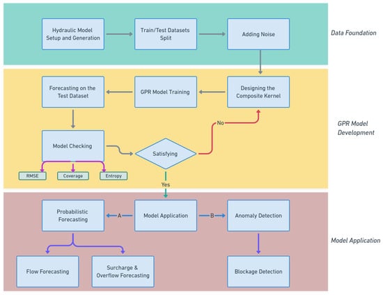
Figure 2.
Flowchart of the research methodology, illustrating the stages from data foundation to the final applications. This process starts from preparing training and test datasets and then makes the composite kernel for the GPR model development. Finally, the built model comes to different applications.
In this case study, the DWF has an average value of 25 L/s, so the 3 standard deviations are set to be 2.5 L/s (standard deviation = 0.8 L/s). It should be noted that the noise level remains the same for all dry- and wet-weather periods for simplicity.
The GPR model can be trained with a single input (only time) and forecast the flow or depth at future time steps (single-input, single-output model) or incorporate other influencing factors in forecasting (multi-input, single-output model). In this study, time as the primary input in the time-series and the precipitation as the key influencing factor are considered as the inputs of the model. The output of the model is the desired flow or depth.
The model can take more factors as inputs (e.g., population, land use, geometry, etc.) to increase the accuracy. Nonetheless, it is important to note that each new factor increases the model’s dimensionality and, consequently, its computational demand which is not preferred in this research.
Once the data from PySWMM are collected and processed, they are imported into a GPR model constructed by the GPflow package in Python [51]. Depending on the data pattern and the dominant features of the time-series, a single or composite kernel, i.e., a combination of multiple covariance functions, is employed to capture different characteristics of the data.
Furthermore, as the wet-weather flow (WWF) is not as predictable as the dry-weather flow (DWF) due to the intense flows entering the sewers after each rainfall in a catchment, ordinary kernels may not fully capture these changes. So, a composite kernel designed to take stormwater and wastewater characteristics into account is needed.
2.4. Kernel Design
The selection of an appropriate kernel, or covariance function, is fundamental to the performance of a GPR model, as it encodes assumptions about the function being modelled. Various methods have been proposed for automatically selecting the optimal kernel for a GP model [52,53]. However, these methods add to the overall complexity of the model significantly which is not desirable in this study.
Moreover, from an overview of the water usage and sewer flow patterns, and the impact of the rainfall magnitude on the flow, it can be understood that the wastewater flow will follow some basic patterns that can be effectively captured within the main GP model by tuning the hyperparameters.
The main kernels used in this research are Periodic and Matérn kernels. Periodic kernel can be formulated as follows [46]:
where l is the length scale, and are GP input vectors.
Matérn kernel family can be formulated as [46]:
where is the modified Bessel function [54]. l is the length scale and ν is a free parameter which is typically selected as 0.5, 1.5, or 2.5. Matérn kernels with higher value of ν are smoother, compared to smaller ν values.
The effectiveness of the designed kernel is assessed by the model checking metrics discussed in Section 2.5.
2.5. Anomaly Detection
To apply the GPR method for anomaly detection in sewer systems, the same training process used in the forecasting model is adopted, using the depths data of each manhole in the hydraulic model. These depth values serve as the training and testing datasets for the GPR model.
In a real-world case, a GPR model is trained using real-time depth measurements from the sensors and precipitation data obtained from the nearest online rain gauges. The trained model predicts expected depth values for each manhole in real-time. By comparing these predicted values with the actual sensor readings, discrepancies can be identified. If deviations exceed predefined thresholds set by the GPR model, an anomaly is detected. Anomalies typically manifest as unusually low or high depth values, indicating potential blockages—either downstream (causing increased water levels) or upstream (leading to sudden drops in depth).
In this study, two months of simulated depth data and precipitation are used as training data and the predictions in each timestep seek anomalies in the next 10 h. The anomaly detection process takes place separately for each manhole but the designed kernel can be used for all datasets.
In many cases, blockages only reduce the capacity of the pipe rather than fully obstructing the flow. Consequently, they do not lead to a surcharge, or a spike change in the depth enough to be flagged as an anomaly. However, GPR model can detect these changes as small deviations that can be considered as probable blockages and be put into inspection plans for early interventions.
The anomaly detection mechanism also considers data resolution. A single outlier may not always indicate an issue, so a predefined number of consecutive data points exceeding the threshold is required to trigger an alarm. The exact criteria can be adjusted based on case-specific conditions.
2.6. Model Checking
The role of predictive model checking is to assess the practical fit of a model [55]. Various techniques exist for assessing the fit of a model including statistic measures [56] and graphical checks [57]. Among them, root mean square error (RMSE), coverage and entropy are selected as three key metrics assessing the GPR model in this study. RMSE, coverage, and entropy together offer a balanced evaluation of the model by capturing its accuracy, the effectiveness of its uncertainty bounds, and the overall reliability of its probabilistic predictions.
2.6.1. Root Mean Square Error
RMSE measures the accuracy of the predictions by calculating the standard deviation of the residuals, providing a straightforward interpretation of the prediction error [58].
where N is the number of test points, is the actual value (flow, depth, etc.), and is the predicted value.
2.6.2. Coverage
Coverage represents the percentage of data points that fall within the defined credible interval of the model. A good model is defined as a model having an α% coverage for an α% credible interval [56]. The typical value for α is 95, which is used in this research as well.
2.6.3. Entropy
Entropy quantifies the uncertainty associated with the predicted distribution, with higher entropy showing greater uncertainty [59]. For a univariate Gaussian probability density function with a variance of σ2, the differential entropy h(t) is given by the formula [60]:
The overall differential entropy of the test points can be calculated as:
This value quantitatively reflects how narrow or wide the bounds are defined. A wider bound can increase the coverage but will result in higher entropy. Thus, a trade-off between these three measures—RMSE, coverage and entropy—is necessary in model evaluation.
It is noteworthy that the differential entropy used in this study is slightly different with the Shannon entropy used for discrete distributions. Unlike Shannon entropy, differential entropy can take negative values when the variance of the data is very small which completely depends on the unit of the data. Therefore, differential entropy values from different models are not directly comparable. Despite this drawback, differential entropy helps identify which kernel configuration provides predictions with lower overall uncertainty, when evaluating different kernel designs using the same training and testing data.
3. Results and Discussion
3.1. Forecasting the WWTP Influent
The inflow of the WWTP is a critical metric for sewer system management, as it significantly influences the performance of the treatment plant. Accurate forecasting of WWTP influent enables proactive decision-making, allowing operators to optimise treatment processes, manage resources effectively, and mitigate potential issues such as overflows. Using a GPR model, flow predictions can be interpreted probabilistically, providing not only point predictions but also a measure of the associated uncertainty.
The WWTP influent values have been derived from the hydraulic simulator (PySWMM). To simulate real-world noise and variability, a zero-mean normal noise with a standard deviation of 0.8 L/s was added to the simulated values.
Once the simulations were complete and the noise was added to the dataset to make the synthetic data more realistic, train and test datasets were prepared and processed to construct the GPR model. The model’s ability to capture the temporal dynamics of the influent, including both DWF patterns and the response to rainfall events, is crucial for effective wastewater management.
Figure 3 illustrates the WWTP influent and precipitation over the study period. The graph highlights the variability in influent flow, demonstrating the influence of rainfall events on peak flow rates. The total precipitation for the year is 875.6 mm.
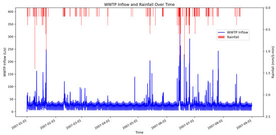
Figure 3.
Simulated WWTP inflow without added noise and the precipitation in the case study. The blue line shows the inflow change overtime and the red line shows the precipitation depth in 5 min intervals.
To build and test the GPR model’s predictions, 6 months of the study period were selected as the training dataset, and the subsequent 2 months for testing. The 6-month period allow the model capture daily, weekly and monthly patterns effectively. The interval between the data points is one hour and the simulation timesteps are 180 s. The results of the GPR model are presented in Figure 4.
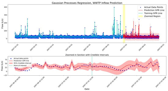
Figure 4.
Gaussian process regression model on 6 months of training and 2 months of test data (top). The regression lines are shown in blue and red for training and test sets, respectively. The first 3 days of the test set is selected for a detailed illustration (bottom).
The bounds illustrate a 95% credible interval of the Gaussian distributions, corresponding to 1.96 standard deviations. Figure 5 illustrates the predicted distribution at a randomly selected point, from the zoomed-in section in Figure 4, showing how the Gaussian distributions work with the data.
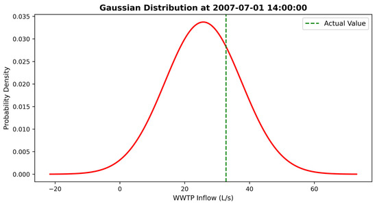
Figure 5.
Gaussian distribution of the predicted WWTP inflow at 2007-07-01 at 14:00 p.m. The green dashed line shows the actual test point value. The distribution’s domain is selected as ±4 standard deviation of the distribution for a better illustration.
As shown in Figure 4, the predictive uncertainty in the GPR model increases as the predictions move further from the training data points, leading to a wider bound around the GPR mean. This occurs because the farther a prediction is from the training set, the less information the model has to constrain it. The mathematical reason behind this fact can be seen in Equation (5). As the distance between and increases, the becomes smaller and the covariance of the predictions achieves higher values. This complies with the fundamental principle that predictions become more uncertain as they extend beyond the observed data points.
The designed kernel for this model consists of four distinct covariance functions. The first two are periodic kernels, selected to capture the hourly and daily variations in the wastewater production pattern. These two kernels target the time input in the training data. The other kernel which is particularly designed to capture rainfall effect on the flow is a Matérn12 kernel (from the gpflow. GPR library in Python). This kernel belongs to the Matérn covariance family with ν = 1/2 that makes the covariance function more rough compared to other ν values [46]. As a result, it can take the spike changes in flow caused by rainfalls.
The final kernel is a noise kernel used to handle the noise in observed data. The noise kernel is a two-dimensional function that is combined with other kernels by a simple addition.
The choice of this kernel structure is supported by model evaluation results and its ability to reproduce the observed data patterns. The model checking shows that over the 2-month test period, Coverage of the model is 99.4% for the 95% credible interval which indicates a perfect coverage. The RMSE between the actual data and the GPR’s mean prediction for this 2-month period is 10.87 L/s. While this value seems high relative to the overall mean flow of 26.16 L/s, it reflects the significant errors that occur during high-magnitude, wet-weather events.
Additionally, the average differential entropy across the test points is 6.19, providing a measure of predictive uncertainty as defined in Section 2.6.3. While differential entropy’s dependence on data scaling means its values are not directly comparable across different datasets and may not translate to an easily interpreted practical metric, it remains useful for model selection within a specific analysis.
The model’s reliability highly depends on the range of values used in the training step. For this model, having rainfall events with greater depth values can train the model better, particularly for predictions at wet-weather periods. As shown in Figure 3 and Figure 4, most of the large rainfalls happen at the 6th month of the year where it is placed in the training zone of the GPR model. To show the importance of the wide span of training data values, the training period is shifted back by one month and the model uses the first five months of the period for training. Hence, the sixth month with its heavy rainfalls is put into the test zone.
The results of this model show that some of the high flow values at the testing zone fall outside predicted bounds which indicates the importance of a representative value range in the training data for achieving accurate predictions. The model checking measures with the same kernel setting indicate 13.82 L/s of RMSE, 98.2% of coverage, and 5.98 of entropy. The increased value of RMSE shows a weaker fit of data which also can be proved by the visual GPR line in the predictions. The entropy and coverage values have not changed significantly; however, outliers exist in the high flow times.
As it is evident in Figure 4, a few outliers exist in the predicted data. These outliers mostly happen in the timesteps when there was an intense rainfall and consequently, a spike change has occurred in the flow. Also, some of the data fall outside the bounds at the starting hours of the prediction when the model is adapting itself with the data and the bounds are narrower than the other predicted timesteps.
Moreover, it is important to note that the fact that Figure 4 and Figure 5 show non-zero probability values for negative flow is due to the natural assumption of GPR that every data point is distributed Gaussian [46]. This can be highly unlikely and can be resolved by incorporating physical constraints. Addressing this limitation is beyond the scope of the current study but will be considered in future work to improve the model’s physical consistency.
3.2. Forecasting Node Surcharges and Overflows
Using the same method, the water level in manholes—where the sensors are usually placed—can also be predicted. These predictions are useful in managing surcharges and overflows. Moreover, since the CSOs are spotlights of the sewer systems and water companies monitor them intently, forecasting CSOs would be another helpful application of GPR.
In this case study, the manhole with the most surcharge and overflow issues has been selected for the GPR forecasting. This selection ensures a sufficient number of data points are available for model evaluation. Also, it aligns with operational priorities, as manholes with persistent issues demand more attention over time. The results of the water depth prediction at the J15 node (the selected manhole) are presented in Figure 6 and Figure 7.
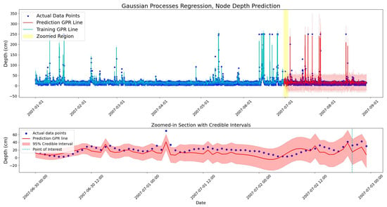
Figure 6.
Water depth forecasting at node J15 for 2 months (top). GPR line at training and test datasets are illustrated in blue and red, respectively. The first 3 days of the test set is selected for a detailed illustration (bottom).
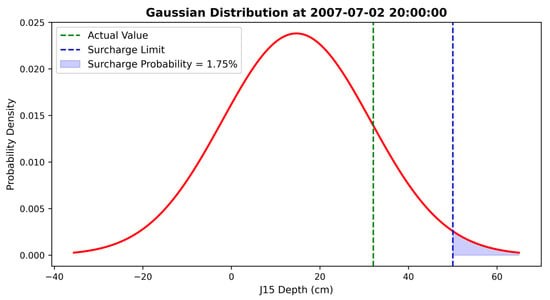
Figure 7.
Gaussian distribution of the predicted node depth on 2007-07-02 at 8:00 p.m. The green dashed line shows the actual test point value. The purple dashed line also indicates the surcharge level which equals the pipe diameter. The area under the distribution for values greater than the surcharge limit is coloured in purple and shows the surcharge probability. The distribution’s domain is selected as ±4 standard deviation of the distribution for a better illustration.
To demonstrate the model’s capability on different but related time series, the same training and testing periods from the WWTP inflow analysis were used. The methodology remains consistent: a separate, single-output GPR model is trained for each manhole of interest, using that specific node’s depth data as the target variable.
Given that the manhole depth is 2.5 m, the maximum observed values reach 250 cm in Figure 6, and the GPR model accounts for this range of variation during training. The results show that although significant rainfall events occurred during the test period, the GPR model does not predict excessively high water depths. This prediction can be restricted to certain values, but the model appears to do well without such constraints.
Since the water level pattern closely resembles the flow pattern, the same composite kernel with tuned length scales and variances has been implemented in the GPR model. The model checking results show that the RMSE of the predictions is 10.9 cm, which is somewhat high compared to the 17.6 cm average water depth in the manhole over time. The coverage of the prediction is 99.4% that shows a perfect performance. Also, the differential entropy is calculated as 6.22.
In Figure 7, a predicted point is randomly selected for illustration. The pipe diameter is 50 cm, and water levels exceeding this threshold cause surcharges in the manhole. This value is marked with a dashed line, and the area under the predictive distribution exceeding this threshold is coloured to indicate the probability of surcharge. In this figure, the surcharge probability is 1.75%, which can be assumed to be negligible. The actual value at this point also confirms that no surcharge happened at this timestep.
This type of probabilistic output can be beneficial for developing a decision-making system which can be used in the water industry. With the same approach employed in finding the surcharge probability, manhole overflow probability can be predicted over time. These probabilistic forecasts allow operators to prioritise maintenance and allocate resources more efficiently, by focusing on locations and times with the highest risk. Figure 8 indicates the probability of surcharges and overflows in the 2-month test period of this case study.
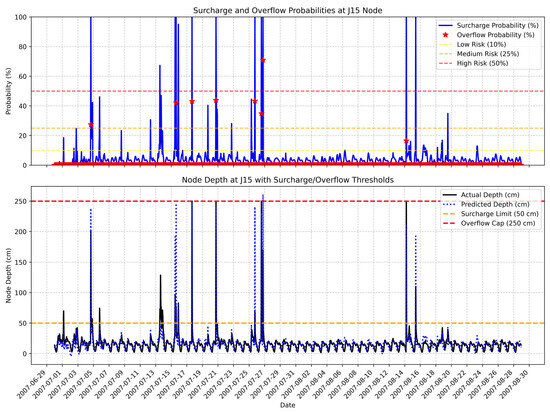
Figure 8.
(Top): the probability of surcharge and overflow in the selected manhole. Blue line shows the probability of surcharge over time, and the red stars show the probability of an overflow from the manhole in each timestep. The dashed lines are drawn to divide the space into low, medium and high-risk zones. (Bottom): actual and predicted water depth at the selected manhole. Surcharge and overflow limits are shown with dashed lines.
In this figure, three thresholds (10, 25 and 50% probability) have been defined to indicate different levels of surcharge/overflow risk. These thresholds were defined based on the actual surcharge events in this case. In real-world scenarios, these thresholds would be defined based on the operator’s specific risk tolerance.
Figure 8 shows one overflow prediction with probability greater than 50% and six predictions with 25 to 50% probability of happening. Among these seven predictions, four test points show that there is an actual overflow and the other three show no overflow. For predictions in the low-risk range, no overflow occurred in the simulation and the forecasts are made accurately.
During the 2-month period of the test period, surcharges occurred in 26 timesteps. The surcharge probability derived from the GPR model assigned different probabilities for each event, as presented in Table 2. Among the 26 surcharges, 5 events were not flagged as high- or medium-risk events while the remaining 21 timesteps were correctly identified with significant probability of surcharge. These surcharges occurred across 11 rainfall events and the model could predict 8 as high-risk and 2 as medium-risk events.
Table 2.
Details of the actual surcharge events and the corresponding predicted probability values.
The same approach can be applied to forecast CSOs in the system. In this case study, the CSO is located downstream of a weir, which receives flow from an upstream manhole with an inlet offset. By predicting the water level at the upstream manhole, it becomes possible to estimate CSO occurrences more effectively. This approach allows the model to run more confidently using a continuous timeseries from the upstream manhole, which spans all training points and contains meaningful variation. In contrast, the CSO flow data contains only a few non-zero values (eight, in the one-year simulation period of this study) during heavy rainfall events, with the majority of timesteps showing zero flow.
Like the flow prediction, Figure 6 and Figure 7 show a probability for negative depth values which seems unrealistic. It also shows non-zero probabilities for water depths exceeding the manhole’s depth, which is physically impossible. The reason behind this matter is that the model is running purely data-driven without any physical constraint. Therefore, for more realistic predictions physical constraints will be added to the model in the future.
3.3. Anomaly Detection
The primary cause of anomaly in sewer systems is the blockage. In this study, an artificial spot, partial blockage is introduced in the C6 conduit of the hydraulic model, located between nodes J2 and J3. This blockage is simulated by increasing the roughness of the pipe instantly. This increase in roughness lowers the ability of the pipe to transfer water; therefore, the flow reduces, upstream depth increases, and downstream depth decreases.
These sudden changes in depth and flow can be considered as anomalies by comparing the observed values with GPR prediction results taken from the previous timesteps. When a sequence of observed values consistently falls outside the credible interval bounds of the predictions, it can serve as a reliable indicator of a potential blockage.
While simpler anomaly detection methods exist, such as fixed-level thresholds, the GPR framework provides a reliable approach by generating dynamic, probabilistic bounds that are conditioned on both time and precipitation, allowing for more sensitive fault detection.
The results of the depth prediction for the J2 node (the upstream manhole) are illustrated in Figure 9. For clarity, only the last two days of the training data from the 2-month training period are shown.
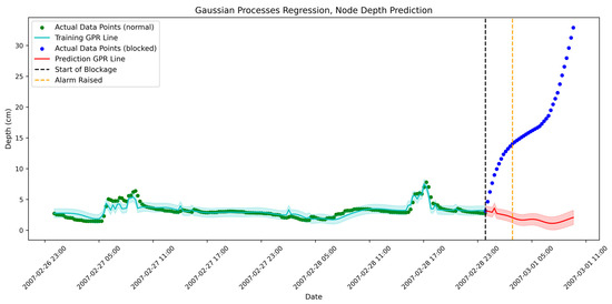
Figure 9.
Blockage detection by water depth forecasting at J2 node. The prediction for 10 h has been presented by red line and the observed values have been presented by blue bullets. After three hours of consequent data points falling outside the bounds, an alarm is raised showing a probable blockage. The time interval between points is 15 min.
As shown in Figure 9, after 3 h of consequent data points falling outside the bounds, an alarm has been raised. This threshold is defined by the authors and can be adjusted based on the data points interval. Lowering this threshold would cause false alarms and lead to an increased inspection cost. However, false alarms are generally preferred over missed blockages [61].
The same approach can be applied to the downstream manhole (J3). Nonetheless, for the nodes receiving flow from multiple sources, blockage in one feeding pipe cannot be detected easily. A promising direction for future research is to use data-driven predictions from pairs of nodes that are directly connected or linked via the shortest paths. This can improve the ability of anomaly detection in the sewer system.
3.4. Prediction with Limited Data
As previously stated, GP models are capable of making predictions with minimal data for the training process and are more reliable in this case compared to other regression and classification methods among data-driven models. To demonstrate this, a flow prediction with one week of data has been made for a 3-day forecasting period. The test period is deliberately selected from the wet-weather periods to capture significant changes in the flow. The results are presented in Figure 10.
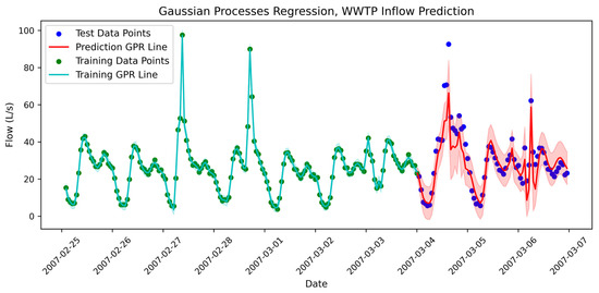
Figure 10.
WWTP inflow prediction with seven days of training data using Gaussian process regression. The test period is three days, and the 95% credible interval is used to show the uncertainty around the predictions.
As the results show, the GPR line is fitted well on the data and the predictions seem reasonable. To further evaluate the model’s robustness, four random 10-day segments were selected from the one-year dataset. The average results across these samples show 91.7% coverage, an RMSE of 8.44 L/s and an entropy of 4.54. These metrics suggest that the model trained with short periods can outperform longer-term models.
The primary limitation of using short training periods is the insufficient number of rainfall events available to train the model effectively. So, if a significant rain event occurs in the test points, the model is incapable of predicting the correct corresponding flow.
3.5. Further Discussion
The rainfall depths that have been used in this research were treated as deterministic inputs. However, in a predictive model, rainfalls will appear as probabilistic values with a likelihood of happening. Therefore, for an improved prediction, rainfall values can be set as Gaussian probability density function, each representing a level of uncertainty.
Moreover, standard GPR assumes Gaussian uncertainty, which may not reflect real-world conditions. This limitation can be addressed by employing more advanced techniques capable of capturing non-Gaussian distributions.
The predictions made in this study were all in a range of short- and medium-term periods because the main goal of this study was to detect flaws and anomalies, and to warn about high or low flows in a sewer system. The long-term predictions can be conducted with the aim of GPs, but the computational costs and high values of uncertainties may make other data-driven models more suitable for asset management applications.
In such cases, a kernel which captures annual cycles of groundwater infiltration can be added to the main kernel to enhance the model. Moreover, population increase and changes in water usage habits should be considered in long-term forecasts.
The GP regression model, shown in Figure 4, is built with hourly data, resulting in 4320 training points. For a more detailed prediction, data of the same period with a 5 min resolution can be used. However, this increases the number of training points to 51,840 which significantly increases the computational cost of the model due to the O(N3) complexity of the GP. In such cases, methods such as Sparse Variational Gaussian Processes (SVGP) can be beneficial in handling the large dataset [62].
It is important to note that rain gauge data is typically not available in real time and often arrives with a delay of 15 min or more. However, this latency does not significantly affect the performance of the anomaly detection model, as the alarm mechanism is designed to trigger only after a defined number of consecutive data points fall outside the credible bounds.
Additionally, the hydraulic simulations in this study were based on a single rain gauge, assuming uniform precipitation across the catchment. Future work should consider using spatially distributed rainfall data, which would provide more realistic and varied runoff inputs for training the GPR model, especially for large catchments.
The model’s performance was defined by three metrics in this research. These metrics can be used separately for dry- and wet-weather periods to better show the model’s performance during extreme events and the baseline.
Finally, incorporating physical constraints into the model can significantly enhance its realism and robustness. For example, the mean function which is commonly assumed to be zero in standard GPR can be replaced with a physics-informed prior that reflects expected system behaviour and is updated during posterior inference. Also, the geometry of a particular manhole, pipe or weir can be considered in producing predicted distributions for more precision.
Additionally, physical constraints, such as the continuity equation or operational limits like minimum flow rates and maximum water depth in each pipe or manhole, can be embedded into the model. These constraints help ensure that predictions remain within realistic and operationally acceptable bounds.
4. Conclusions
In this study, Gaussian processes regression (GPR) was implemented to predict flow and depth in a sewer system and flag anomalies. The case study was a hypothetical skeleton sewer system with different characteristics of a real-world system serving 11,300 inhabitants of a city in the UK.
The framework’s novelty lies in its custom composite kernel, designed to capture key sewer flow dynamics, and its application for real-time blockage detection using predictive uncertainty bounds. The approach demonstrated high performance even when trained on limited data, highlighting its potential for real-world deployment in forecasting and real-time control, especially when historical data is sparse.
Based on the findings in sewer flow prediction, taking time and precipitation as two main inputs of the GPR model effectively captures flow patterns with the designed kernel. In contrast, having a single-input model cannot effectively reflect flow changes during wet-weather periods. Also, adding new inputs to the model only adds to the dimension of the covariance matrix, which is directly related to the computational cost of the GPs.
Designing a composite kernel that reflects the underlying physical processes in the system proved highly effective in this model. The kernel was optimised by maximising the log marginal likelihood, while additional evaluation metrics such as RMSE, coverage, and differential entropy helped identify the best kernel settings.
GPR can respond well to minimal training datasets and make reliable predictions. On the other hand, a high number of data points can reduce the model’s speed and make it computationally inefficient.
Outliers may appear in every prediction, often due to a lack of wide range in training datasets, especially when dealing with precipitation data. In such cases, increasing the length of the training period helps.
The proposed probabilistic framework offers a new way for decision-makers to assess sewer system risks. By providing dynamic uncertainty bounds for its forecasts, the model allows for a quantitative assessment of risk (e.g., overflow probability), which can support more resilient infrastructure planning and help mitigate threats to public health and the environment.
In summary, this research offers a promising framework for probabilistic forecasting and anomaly detection in sewer systems. Future work can enhance this approach by incorporating physical constraints into the model and representing input variables, such as rainfall, as probability distributions to capture input uncertainty more accurately. Furthermore, this probabilistic platform has the potential to serve as an alternative to real-time control and forecasting platforms currently used by water companies, offering a transparent and adaptable decision-support tool.
Author Contributions
Conceptualisation, M.R., H.R. and P.M.-S.; methodology, M.R. and H.R.; software, M.R.; validation, M.R.; formal analysis, M.R.; investigation, M.R. and H.R.; resources, M.R., H.R. and P.M.-S.; data curation, M.R.; writing—original draft preparation, M.R.; writing—review and editing, M.R., H.R. and P.M.-S.; visualisation, M.R.; supervision, H.R. and P.M.-S.; project administration, H.R. All authors have read and agreed to the published version of the manuscript.
Funding
This research received no external funding.
Data Availability Statement
The hydraulic model and the source code for forecasting flow are available through the GitHub repository: https://github.com/MohsenRz/Sewer_System_Forecasting_Emulator.git, accessed on 20 July 2025.
Acknowledgments
For the purpose of open access, the author has applied a Creative Commons Attribution (CC BY) licence to any Author Accepted Manuscript version arising from this submission.
Conflicts of Interest
The authors declare no conflicts of interest.
Abbreviations
The following abbreviations are used in this manuscript:
| CSO | Combines Sewer Overflow |
| GP | Gaussian Process |
| GPR | Gaussian Processes Regression |
| SWMM | Storm Water Management Model |
| DWF | Dry-weather Flow |
| CCTV | Closed-circuit Television |
| RMSE | Root Mean Square Error |
| SVGP | Sparse Variational Gaussian Processes |
References
- Walski, T.M.; Barnard, T.E. Wastewater Collection System Modeling and Design; Haestad Press: Waterbury, CT, USA, 2004. [Google Scholar]
- Owolabi, T.A.; Mohandes, S.R.; Zayed, T. Investigating the impact of sewer overflow on the environment: A comprehensive literature review paper. J. Environ. Manag. 2022, 301, 113810. [Google Scholar] [CrossRef] [PubMed]
- Perry, W.B.; Ahmadian, R.; Munday, M.; Jones, O.; Ormerod, S.J.; Durance, I. Addressing the challenges of combined sewer overflows. Environ. Pollut. 2024, 343, 123225. [Google Scholar] [CrossRef]
- Arthur, S.; Crow, H.; Pedezert, L. Understanding blockage formation in combined sewer networks. Proc. Inst. Civ. Eng.-Water Manag. 2008, 161, 215–221. [Google Scholar] [CrossRef]
- Faris, N.; Zayed, T.; Aghdam, E.; Fares, A.; Alshami, A. Real-time sanitary sewer blockage detection system using IoT. Measurement 2024, 226, 114146. [Google Scholar] [CrossRef]
- Balla, K.M.; Bendtsen, J.D.; Schou, C.; Kallesøe, C.S.; Ocampo-Martinez, C. A learning-based approach towards the data-driven predictive control of combined wastewater networks–An experimental study. Water Res. 2022, 221, 118782. [Google Scholar] [CrossRef] [PubMed]
- Perez, G.; Gomez-Velez, J.D.; Grant, S.B. The sanitary sewer unit hydrograph model: A comprehensive tool for wastewater flow modeling and inflow-infiltration simulations. Water Res. 2024, 249, 120997. [Google Scholar] [CrossRef]
- Zhang, Q.; Li, Z.; Snowling, S.; Siam, A.; El-Dakhakhni, W. Predictive models for wastewater flow forecasting based on time series analysis and artificial neural network. Water Sci. Technol. 2019, 80, 243–253. [Google Scholar] [CrossRef]
- Li, S.; Tian, W.; Yan, H.; Zeng, W.; Tao, T.; Xin, K. Modeling transient mixed flows in sewer systems with data fusion via physics-informed machine learning. Water Res. X 2024, 25, 100266. [Google Scholar] [CrossRef]
- Stieglitz, M.; Hobbie, J.; Giblin, A.; Kling, G. Hydrologic modeling of an arctic tundra watershed: Toward Pan-Arctic predictions. J. Geophys. Res.-Atmos. 1999, 104, 27507–27518. [Google Scholar] [CrossRef]
- Donnelly, J.; Daneshkhah, A.; Abolfathi, S. Forecasting global climate drivers using Gaussian processes and convolutional autoencoders. Eng. Appl. Artif. Intell. 2024, 128, 107536. [Google Scholar] [CrossRef]
- Machac, D.; Reichert, P.; Rieckermann, J.; Albert, C. Fast mechanism-based emulator of a slow urban hydrodynamic drainage simulator. Environ. Model. Softw. 2016, 78, 54–67. [Google Scholar] [CrossRef]
- Troutman, S.C.; Schambach, N.; Love, N.G.; Kerkez, B. An automated toolchain for the data-driven and dynamical modeling of combined sewer systems. Water Res. 2017, 126, 88–100. [Google Scholar] [CrossRef] [PubMed]
- Ge, J.; Li, J.; Qiu, R.; Shi, T.; Zhang, C.; Huang, Z.; Yuan, Z. A data-driven method for estimating sewer inflow and infiltration based on temperature and conductivity monitoring. Water Res. 2024, 261, 122002. [Google Scholar] [CrossRef] [PubMed]
- Aliashrafi, A.; Zhang, Y.; Groenewegen, H.; Vanrolleghem, P.A. A Review of Data-Driven Modelling in Drinking Water Treatment. Rev. Environ. Sci. Biotechnol. 2021, 20, 985–1009. [Google Scholar] [CrossRef]
- Swiler, L.P.; Gulian, M.; Frankel, A.L.; Safta, C.; Jakeman, J.D. A survey of constrained Gaussian process regression: Approaches and implementation challenges. J. Mach. Learn. Model. Comput. 2020, 1, 119–156. [Google Scholar] [CrossRef]
- Raissi, M.; Perdikaris, P.; Karniadakis, G.E. Physics-informed neural networks: A deep learning framework for solving forward and inverse problems involving nonlinear partial differential equations. J. Comput. Phys. 2019, 378, 686–707. [Google Scholar] [CrossRef]
- Thorndahl, S.; Willems, P. Probabilistic modelling of overflow, surcharge and flooding in urban drainage using the first-order reliability method and parameterization of local rain series. Water Res. 2008, 42, 455–466. [Google Scholar] [CrossRef]
- Breinholt, A. Uncertainty in Prediction and Simulation of Flow in Sewer Systems. Ph.D. Thesis, Technical University of Denmark, Kongens Lyngby, Denmark, 2012. [Google Scholar]
- Raimondi, A.; Sanfilippo, U.; Becciu, G. Uncertainty on flow rate and temperature measurement for the detection of illicit flows in sewers. J. Hydrol. 2024, 632, 130891. [Google Scholar] [CrossRef]
- Sriwastava, A.K.; Tait, S.; Schellart, A.; Kroll, S.; Van Dorpe, M.; Van Assel, J.; Shucksmith, J. Quantifying uncertainty in simulation of sewer overflow volume. J. Environ. Eng. 2018, 144, 04018050. [Google Scholar] [CrossRef]
- Ding, C.; Rappel, H.; Dodwell, T. Full-field order-reduced Gaussian Process emulators for nonlinear probabilistic mechanics. Comput. Methods Appl. Mech. Eng. 2023, 405, 115855. [Google Scholar] [CrossRef]
- Wang, J. An intuitive tutorial to Gaussian process regression. Comput. Sci. Eng. 2023, 25, 4–11. [Google Scholar] [CrossRef]
- Ding, C.; Chen, Y.; Rappel, H.; Dodwell, T. Functional order-reduced Gaussian Processes based machine-learning emulators for probabilistic constitutive modelling. Compos. Part A Appl. Sci. Manuf. 2023, 173, 107695. [Google Scholar] [CrossRef]
- Gonzalvez, J.; Lezmi, E.; Roncalli, T.; Xu, J. Financial applications of Gaussian processes and Bayesian optimization. arXiv 2019, arXiv:1903.04841. [Google Scholar] [CrossRef]
- Roberts, S.; Osborne, M.; Ebden, M.; Reece, S.; Gibson, N.; Aigrain, S. Gaussian processes for time-series modelling. Philos. Trans. R. Soc. A Math. Phys. Eng. Sci. 2013, 371, 20110550. [Google Scholar] [CrossRef]
- Sun, A.Y.; Wang, D.; Xu, X. Monthly streamflow forecasting using Gaussian process regression. J. Hydrol. 2014, 511, 72–81. [Google Scholar] [CrossRef]
- Pastrana-Cortés, J.D.; Gil-Gonzalez, J.; Álvarez-Meza, A.M.; Cárdenas-Peña, D.A.; Orozco-Gutiérrez, Á.A. Scalable and interpretable forecasting of hydrological time series based on variational Gaussian processes. Water 2024, 16, 2006. [Google Scholar] [CrossRef]
- Samuelsson, O.; Björk, A.; Zambrano, J.; Carlsson, B. Gaussian process regression for monitoring and fault detection of wastewater treatment processes. Water Sci. Technol. 2017, 75, 2952–2963. [Google Scholar] [CrossRef]
- Ng, J.Y.; Fazlollahi, S.; Dechesne, M.; Soyeux, E.; Galelli, S. Robust optimal design of urban drainage systems: A data-driven approach. Adv. Water Resour. 2023, 171, 104335. [Google Scholar] [CrossRef]
- Wang, Y.; Ocampo-Martinez, C.; Puig, V. Stochastic model predictive control based on Gaussian processes applied to drinking water networks. IET Control. Theory Appl. 2016, 10, 947–955. [Google Scholar] [CrossRef]
- Grbić, R.; Kurtagić, D.; Slišković, D. Stream water temperature prediction based on Gaussian process regression. Expert Syst. Appl. 2013, 40, 7407–7414. [Google Scholar] [CrossRef]
- Bonakdari, H.; Ebtehaj, I.; Samui, P.; Gharabaghi, B. Lake water-level fluctuations forecasting using minimax probability machine regression, relevance vector machine, Gaussian process regression, and extreme learning machine. Water Resour. Manag. 2019, 33, 3965–3984. [Google Scholar] [CrossRef]
- Sweetapple, C.; Webber, J.; Hastings, A.; Melville-Shreeve, P. Realising smarter stormwater management: A review of the barriers and a roadmap for real world application. Water Res. 2023, 244, 120505. [Google Scholar] [CrossRef] [PubMed]
- Patil, R.R.; Calay, R.K.; Mustafa, M.Y.; Ansari, S.M. AI-driven high-precision model for blockage detection in urban wastewater systems. Electronics 2023, 12, 3606. [Google Scholar] [CrossRef]
- Rosin, T.R.; Kapelan, Z.; Keedwell, E.; Romano, M. Near real-time detection of blockages in the proximity of combined sewer overflows using evolutionary ANNs and statistical process control. J. Hydroinf. 2022, 24, 259–273. [Google Scholar] [CrossRef]
- Jimoh, M.; Abolfathi, S. Modelling pollution transport dynamics and mixing in square manhole overflows. J. Water Process Eng. 2022, 45, 102491. [Google Scholar] [CrossRef]
- Li, N.; Wang, X.; Li, Z.; Zhao, F.; Nair, A.; Zhang, J.; Liu, C. Real-time identification and positioning of sewer blockage based on liquid level analysis in rural area. Processes 2023, 11, 161. [Google Scholar] [CrossRef]
- Kargar, K.; Joksimovic, D. Analysis of sewer blockage causes using open data. Water Pract. Technol. 2024, 19, 3855–3866. [Google Scholar] [CrossRef]
- Rossman, L.A.; Simon, M.A. Storm Water Management Model User’s Manual Version 5.2; US Environmental Protection Agency: Cincinnati, OH, USA, 2022. [Google Scholar]
- Prodanovic, P.; Simonovic, S.P. Development of Rainfall Intensity Duration Frequency Curves for the City of London under the Changing Climate; Department of Civil and Environmental Engineering, The University of Western Ontario: London, ON, Canada, 2007. [Google Scholar]
- Rezaee, M.; Tabesh, M. Effects of inflow, infiltration, and exfiltration on water footprint increase of a sewer system: A case study of Tehran. Sustain. Cities Soc. 2022, 79, 103707. [Google Scholar] [CrossRef]
- Zeydalinejad, N.; Javadi, A.A.; Webber, J.L. Global perspectives on groundwater infiltration to sewer networks: A threat to urban sustainability. Water Res. 2024, 262, 122098. [Google Scholar] [CrossRef]
- McDonnell, B.E.; Ratliff, K.; Tryby, M.E.; Wu, J.J.X.; Mullapudi, A. PySWMM: The python interface to stormwater management model (SWMM). J. Open Source Softw. 2020, 5, 1–3. [Google Scholar] [CrossRef] [PubMed]
- Stovin, V. Mappin Green Roof Test Bed Rainfall and Runoff Data 2007; The University of Sheffield: Sheffield, UK, 2024. [Google Scholar] [CrossRef]
- Rasmussen, C.E.; Williams, C.K.I. Gaussian Processes for Machine Learning; MIT Press: Cambridge, MA, USA, 2006. [Google Scholar]
- Deshpande, S.; Rappel, H.; Hobbs, M.; Bordas, S.P.; Lengiewicz, J. Gaussian process regression + deep neural network autoencoder for probabilistic surrogate modeling in nonlinear mechanics of solids. Comput. Methods Appl. Mech. Eng. 2025, 437, 117790. [Google Scholar] [CrossRef]
- Rappel, H.; Beex, L.A.; Hale, J.S.; Noels, L.; Bordas, S.P. A tutorial on Bayesian inference to identify material parameters in solid mechanics. Arch. Comput. Methods Eng. 2020, 27, 361–385. [Google Scholar] [CrossRef]
- Duvenaud, D. Automatic Model Construction with Gaussian Processes. Ph.D. Thesis, University of Cambridge, Cambridge, UK, 2014. [Google Scholar]
- Wilson, A.G. Covariance Kernels for Fast Automatic Pattern Discovery and Extrapolation with Gaussian Processes. Ph.D. Thesis, University of Cambridge, Cambridge, UK, 2014. [Google Scholar]
- Matthews, A.G.; Van Der Wilk, M.; Nickson, T.; Fujii, K.; Boukouvalas, A.; Le, P.; Ghahramani, Z.; Hensman, J. GPflow: A Gaussian process library using TensorFlow. J. Mach. Learn. Res. 2017, 18, 1–6. [Google Scholar]
- Duvenaud, D.; Lloyd, J.; Grosse, R.; Tenenbaum, J.; Ghahramani, Z. Structure Discovery in Nonparametric Regression through Compositional Kernel Search. In Proceedings of the International Conference on Machine Learning, Atlanta, GA, USA, 26 May 2013; pp. 1166–1174. [Google Scholar]
- Kuok, S.C.; Yao, S.A.; Yuen, K.V.; Yan, W.J.; Girolami, M. Bayesian generative kernel Gaussian process regression. Mech. Syst. Signal Process. 2025, 227, 112395. [Google Scholar] [CrossRef]
- Abramowitz, M.; Stegun, I.A. (Eds.) Handbook of Mathematical Functions with Formulas, Graphs, and Mathematical Tables; US Government Printing Office: Washington, DC, USA, 1948. [Google Scholar]
- Gilks, W.R.; Richardson, S.; Spiegelhalter, D. (Eds.) Markov Chain Monte Carlo in Practice; CRC Press: Boca Raton, FL, USA, 1995. [Google Scholar]
- Malde, S. Gaussian Process Emulators in Coastal Wave Modelling. Ph.D. Thesis, University of Sheffield, Sheffield, UK, 2018. [Google Scholar]
- Gelman, A.; Carlin, J.B.; Stern, H.S.; Rubin, D.B. Bayesian Data Analysis, 3rd ed.; Chapman and Hall/CRC: Boca Raton, FL, USA, 2021. [Google Scholar]
- Hyndman, R.J.; Koehler, A.B. Another look at measures of forecast accuracy. Int. J. Forecast. 2006, 22, 679–688. [Google Scholar] [CrossRef]
- Hasegawa, Y.; Nishiyama, T. Thermodynamic entropic uncertainty relation. arXiv 2025, arXiv:2502.06174. [Google Scholar] [CrossRef]
- MacKay, D.J. Information Theory, Inference and Learning Algorithms; Cambridge University Press: Cambridge, UK, 2003. [Google Scholar]
- Roghani, B.; Cherqui, F.; Ahmadi, M.; Le Gauffre, P.; Tabesh, M. Dealing with uncertainty in sewer condition assessment: Impact on inspection programs. Autom. Constr. 2019, 103, 117–126. [Google Scholar] [CrossRef]
- Liu, H.; Ong, Y.S.; Shen, X.; Cai, J. When Gaussian process meets big data: A review of scalable GPs. IEEE Trans. Neural Netw. Learn. Syst. 2020, 31, 4405–4423. [Google Scholar] [CrossRef]


Disclaimer/Publisher’s Note: The statements, opinions and data contained in all publications are solely those of the individual author(s) and contributor(s) and not of MDPI and/or the editor(s). MDPI and/or the editor(s) disclaim responsibility for any injury to people or property resulting from any ideas, methods, instructions or products referred to in the content. |
© 2025 by the authors. Licensee MDPI, Basel, Switzerland. This article is an open access article distributed under the terms and conditions of the Creative Commons Attribution (CC BY) license (https://creativecommons.org/licenses/by/4.0/).